Download A system for fault diagnosis and simulation of VHDL descriptions

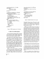
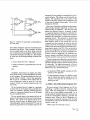
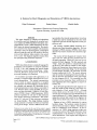
A System for Fault Diagnosis and Simulation of VHDL descriptions
Vijay Pitchumani
Pankaj Mayor
Nimish Ftadia
Department of Electrical and Computer Engineering
Syracuse University, Syracuse NY 13244.
Abstract
This paper describes a compiler and algorithms
for simulation and fault diagnosis of computer hardware modeled in VHSIC Hardware Description Language(VHDL). Given a VHDL description, the compiler creates an internal representation. For simulation, a discrete-event based compiled code simulation
algorithm is used. For fault diagnosis, a hierarchical
approach using the stuck-at fault model a t the first
level and the arbitrary failure model at the second
level, is used. The diagnosis algorithm reasons from
first principles using constraint suspension.
1. Introduction
VHDL has already become a standard language for
specification and simulation of computer hardware
[1,2,3,4]. It is a rich language that permits design
description at several levels of abstraction - behavioral level, RTL level, and gate level. It also permits
structural hierarchy to be described.
For simulation and other CAD applications, it is
necessary to compile VHDL descriptions into an internal representation. The internal representation
may be meant to support interpretive or compiled
code approach. For runtime efficiency we have chosen
the compiled code approach [5]. Specifically the internal representation we have chosen is executable C
code. We have chosen a subset of VHDL for our purposes, and have developed a VHDL to C Code Generator (VCCG). Given a VHDL description, VCCG
produces equivalent C code and C data structures
that capture connectivity information. This combination of C code and C data structures constitutes
our design database. The design database contains
enough pointers to facilitate forward and backward
tracing of the design. VCCG is different from existPermission to copy without fee all or part of this material is granted
provided that the copies are not made or distributed for direct commercial
advantage, the ACM copyright notice and the title of the publication and
its date appear, and notice is given that copying is by permission of the
Association for Computing Machinery. To copy otherwise, or to republish,
requires a fee and/or specific permission.
ing compilers; the internal representation it produces
is useful not only for simulation but for other CAD
application tools such as fault diagnosis and test generation as well.
The currently available VHDL simulators use a
discrete-event based simulation algorithm. We have
developed a VHDL simulator (VSIM), which uses a
discrete-event based compiled code simulation algorithm.
The concept of fault diagnosis of computer hardware is not new. There are many AI-based and nonAI-based approaches. Within AI, there are two approaches for fault diagnosis. The first approach uses
“rules”. Each rule specifies a symptom/fault pairing [6,7,8,9]. Such rules are created for each design.
Given a set of symptoms, these rules give a set of possible faults for a particular design. As the complexity
of VLSI designs increases, the rule-based approach
becomes impractical [10,11]. The second approach
uses the concept of reasoning from first principles. It
uses the structure and behavior of the given design
for fault diagnosis [10,11]. The reasoning from first
principles is time consuming. Some modifications of
these algorithms have been suggested to improve efficiency [121.
Some AI-based algorithms for fault diagnosis consider only stuck-at fault model [7], while some consider hierarchy of fault models [ 10,11]. Although
stuck-at faults accouiit for most of the faults in the
circuits, they are not the only type of faults which can
cause misbehavior [ll].Hence, diagnosis algorithms
using only stuck-at fault model fail to diagnose the
design if it has faults other than stuck-at faults [ll].
Suppose we have a VHDL description for a given
hardware design. The hardware consists of physical
devices which are subject to failure. This failure can
lead to a misbehavior of the hardware. As the description is in VHDL, design engineers might want
to locate the portion of the VHDL description whose
implementation in the hardware is causing the observed misbehavior. This requires fault diagnosis of
28th ACM/IEEE Design Automation Conference”
Paper 10.2
144
1991 ACM 0-89791-395-7/91/0006/0144 $1.50
VlIDL descriptions.
So far no tools have been available to do fault diagnosis on VHDL descriptions. We have developed a
VHDL Fault DiagnosisTool (VFDT). Given a VHDL
design description and a set of test cases, VFDT intelligently tries to isolate the fault to one or more
VHDL constructs., VFDT assumes a single point of
failure and uses ’both the stuck-at fault model and
the arbitrary fault model. The diagnosis is performed
hierarchically using constraint suspension. The fault
diagnosis approach we have developed for VFDT is
a modified version of Davis’s [ll] approach.
VSIM and VFDT are capable of handling both
combinational and sequential circuits. However,
VFDT requires that latches be controllable and observable; input vectors and observed outputs are
stated in terms of latches as well as primary inputs
(PI’S) and primary outputs (PO’s).
2.
VCCG
L
Sum
Cin
I
Figure 1: A 1-bit adder
- The VHDL Compiler
We have chosen a subset of VHDL for fault diagnosis and simulation. The subset is large enough to
represent any digital system. The main features of
this subset are: (a) concurrent statements, (b) sequential statements, except wait statement, (c) component instantiation and configuration specification
statement, and (d) libraries. The details of this subset are given in [13].
C subroutines. Even if there are multiple instances
of a concurrent statement (by virtue of multiple component instances) only one copy of the corresponding C code will exist. However, as mentioned before
there will be a separate data area for each instance.
Thus different instances of a concurrent statement
will share C subroutines to process a set of data values associated with them.
VCCG represents each concurrent VHDL statement and any of its instances as a C structure in the
design database. Memory is allocated to represent
this structure. This way, each instance of a concurrent VHDL statement has memory to store the data
values associated with it. For example, consider the
I-bit adder shown in Fig. 1 and its corresponding
description in VHDL in Fig. 2. In this example, the
architecture body of the adder uses two instances X1
and X2 of the entity xor. The VHDL description of
the xor gate is given in Fig. 3. For such cases, the entity informations related to X1 and X2 are stored in
separate memory areas. Similarly, the architecture
informations related to X1 and X2 are also stored
in separate memory locations. Similarly, all other
concurrent statements and their instances are represented as C structures. This methodology facilitates
implementation of multiple instances of any concurrent VHDL statement.
We define a 9-process (“generalized process”) to be
a process statement or any concurrent VHDL statement which can be mapped to an equivalent VNDL
process statement. Given any VHDL description, we
will represent it as a network of g-processes. For the
1-bit adder described in Fig. 2, we have a g-process
corresponding to each concurrent statement as seen
in Fig. 4. X1 and X2, the xor gate instantiations
each have 3 concurrent signal assignment statements
as seen from Fig. 3, contributing g-processes gpl-gp3
and gp4-gp6 respectively. The two concurrent signal
assignment statements in the architecture body of
the adder contribute g-processes gp7 and gp8. The
process statement P contributes g-process gp9. This
network of g-processes is used by the simulation and
the fault diagnosis tools.
The computations associated with a VHDL concurrent statement (process statement, concurrent
signal assignment statement, etc) are transformed by
VCCG into a sequence of C statements and stored as
A g-process is an atomic construct for the siniulation and the fault diagnosis tools. Each g-process is
represented as C subroutines as described previously.
The VHDL description is simulated by executing the
C subroutines associated with its g-processes. For
fault diagnosis using the arbitrary fault model, the
diagnostic resolution is limited to a g-process.
Paper 10.2
145
-the entity description for a 1 bit adder
entity adder is
port(A, B, Cin : in bit;
Sum, Cout: out bit);
end adder ;
-an architecture description for a 1 bit adder
architecture mixed of adder is
component xor-gate port ( X, Y: in bit;
Z : out bit) ;
for X1, X2: xor-gate
use entity gates.xor(xorarch) ;
port map(In1 + X , In2 3 Y, Out =+ Z);
signal L, M, N : bit ;
begin
X1: xor-gate port map (A, B, L);
X2: xor-gate port map (L, Cin, Sum);
M e L and C ;
N+AandB;
P: process(M,N )
begin
Carry e M or N ;
end process ;
end mixed;
Figure 2: VHDL description of a 1-bit adder
3. VSIM
- The VHDL Simulator
We have developed a simulator [13] for simulating
circuits described in VHDL. VSIM is capable of simulating the chosen subset of VHDL. It handles high
level as well as hierarchical designs in VHDL.
The elaboration of a design hierarchy produces a
model which is a network of g-processes. Given the
VHDL description (Fig. 2) of the adder in Fig. 1,
the components in the top level design entity are
instantiated and a network of g-processes, as seen
in Fig. 4, is created. This is done by VLINK the VHDL Linker. Simulation involves execution of
these interacting g-processes. VSIM’s kernel coordinates the activity of the g-processes during a simulation. It propagates and updates signal values. It
is also responsible for detecting events that occur,
and for causing appropriate g-processes to execute
in response to these events.
VSIM is an event driven simulator. It maintains
a driver for each signal of each g-process. Each
driver of a signal is a source of values for that signal.
Transactions (signal changes) that are created by a
g-process for a signal are put in the driver queue of
Paper 10.2
146
-the entity description for the XOR gate
entity xor is
port(In1, In2 : in bit; Out: out bit);
end xor;
-an architecture for the above XOR gate
architecture xor-arch of xor is
signal S1, S2 : bit;
begin
S1 G (not I n l ) and In2;
S2 e In1 and (not In2);
Out
S l or S2;
end xor-arch;
Figure 3: VHDL description of an xor gate
that signal of that g-process. Obviously, if a signal
is shared by several g-processes, it will have multiple drivers, one per g-process. This implementation
facilitates the use of resolved signals - signals that
have more than one source.
VHDL has a two-stage model of time referred to
as the simulation cycle. It is based on a generalized
model of the stimulus and response behavior of digital hardware. The g-processes respond to activity on
their inputs with a response on their outputs. During the first stage of the simulation cycle new values
scheduled to take effect at that time are assigned to
signals and are propagated to their sinks. All the
signals scheduled to obtain new values at the current
simulation time are updated. Changes in the values
of these signals could cause some g-processes to become sensitized. During the second stage of the simulation cycle, the sensitized g-processes are executed
till they are suspended. Execution of a g-process
may create transactions on signals which are put on
the corresponding driver queues. At the completion
of the simulation cycle, the simulation clock is set
to the time-stamp of the earliest transaction that is
scheduled to occur. Then the cycle is repeated.
4. Fault Diagnosis by Constraint Suspension
Constraint suspension is a way of diagnosing faults
by reasoning from first principles using knowledge of
the structure and behavior of the circuit. The diagnosis is performed hierarchically by gradually relaxing the assumptions about the failure modes of the
circuit.
Based on an engineer’s notion of-things that can
go wrong, categories of failure are defined. Amongst
erroneous PO can possibly be responsible for the incorrect behavior. This defines a set of potential candidates. The candidates are in the context of the
domain of the fault category being considered; that
is, they may be signals or g-processes. This is called
discrepancy detection.
‘ri=
Figure 4: Network of g-processes corresponding to
the 1-bit adder
these failure categories, some are encountered more
frequently than others. These categories of failure
can be ordered based on the above metric with the
more commonly occurring category of failure preceding the less commonly occurring one. For example
we could have the following ordering of failure categories:
0
0
stuck-at faults (for level 1 diagnosis)
change in behavior of g-processes (for level 2 diagnosis)
Once a set of potential candidates has been generated we apply constraint suspension to them to determine if they are consistent - that is if they could
explain the observed behavior. In general, a signal
or a g-process imposes a relation (or constraints) between its inputs and outputs. When we do constraint
suspension for a candidate, we disable the constraints
associated with it. This amounts to disconnecting
the candidate’s outputs from the candidate so that
these outputs, which are now pseudo-PI’S, are free
to assume any value necessary to cause the observed
values on the PO’s. Procedurally, we assign the given
primary input values to thePI’s and the observed primary output values t o the PO’s. Then we determine
if there is an assignment of values to the pseudo-PI’S
that will cause the circuit to reach a consistent state.
If there is such an assignment, the candidate continues to remain a candidate; otherwise we conclude
that the candidate cannot account for the symptoms.
Clearly, this approach differs from traditional fault
diagnosis methods in that it reasons from first principles and is general enough to permit arbitrary failure
of a g-process. The algorithm presented in this paper is essentially the same as that of [ll];however it
differs from [ll]in the following ways:
etc
Candidates, faults which can explain the misbehavior of the circuit, are first generated for the stuckat fault category. We assume initially that the components behave correctly. Only if this assumption
fails to give us a candidate which explains the observed misbehavior, would we move on to the next
category of faults and perform diagnosis under this
new model.
We use transitive fanin of a signal or a g-process
to denote the set of all signals and g-processes from
which it is reachable. Similarly, transitive fanovt of
a signal or a g-process denotes the set of all signals
that are reachable from it.
The two central issues to this method of fault diagnosis are discrepancy detection and constraint suspension. For a given set of primary inputs, if any
observed primary output is different from the corresponding good machine (predicted) PO, only the
signals and g-processes in the transitive fanin of this
it introduces VHDL specific concepts and techniques into the algorithm
it uses simulation oriented, but efficient, methods for inferencing thereby making use of the
compiled code generated for simulation for inferencing as well
5. VFDT
- The VHDL Fault Diagnosis Tool
We have developed a fault diagnosis tool [14] implementing a modified constraint suspension algorithm, which will intelligently try to diagnose the
fault to one or more signals or g-processes. In an
actual hardware implementation there need not be a
one-bone correspondence between g-processes and
hardware units. When the fault is diagnosed to a
g-process gp, the physical meaning is that the fault
lies somewhere within the set of hardware units which
together contain gp.
VFDT accepts the following as input:
Paper 10.2
147
0
a design description in VHDL
test data - applied test vectors and the observed
responses of the circuit
It will return a set of either signals or g-processes or
both which could consistently explain the erroneous
behavior of the circuit.
In general the test data available to VFDT may
contain many test vectors. Ideally VFDT should
be able to resolve the fault location to a signal or
a g-process. In general diagnostic resolution will increase with the number of test cases. VFDT itself
will not generate tests t o narrow the set of candidates.
VFDT deals with single point of failure fault models and performs fault diagnosis hierarchically. First
it tries to locate the fault assuming the stuck-at fault
model. Failing this, it relaxes the assumption that
the g-processes are behaving correctly and allows
them to fail in any arbitrary way - that is, their
truth table may change in any way. Hence, the second level fault model is called the arbitrary-failure
model. This takes into account the fact that the
module may fail in any arbitrary way. This is a very
comprehensive model and would cover most of the
faults in the circuit.
There are three broad steps in the algorithm. We
will discuss each of them individually.
5.1 Test case selection
From the fault diagnosis point of view, a test case
(i.e. an input test vector and the corresponding observed output) is useful, if any of the observed and
expected PO’s are different. The test case selection
module takes each given test case and simulates it
using VSIM. If the observed output is not identical
to the simulated (good machine) output, VFDT accepts the test case; otherwise VFDT rejects the test
case. If a test case is accepted, the good machine
simulation values at each signal are saved for future
use.
An interesting point to note about the test cases
is that it is not necessary to specify all PI’S and all
PO’s. It is possible to leave some of them unspecified. This is particularly useful when dealing with
sequential circuits.
5.2 Topological candidate generation
The next phase in fault diagnosis is topological candidate generaiion. Initially the set S of candidates
Paper 10.2
148
includes all the signals or all the g-processes in the
circuit. After a test case is accepted by the test case
selection module, the PO’s which have a discrepancy
between the observed and the predicted values are
identified. For each of these erroneous PO’s, the set
SNEW of signals or g-processes that are in its transitive fanin is computed. The intersection of S and
SNEW is placed in S. The modified set S contains the
current candidates. Since we are assuming a single
point of failure, the candidates thus generated should
be in the transitive fanin of all of the erroneous PO’s.
The sets S and SNEW are not computed explicitly,
nor is the intersection performed explicitly. To save
processing time, we use a counter COUNT for each
stuck-at fault (for level 1 diagnosis) or g-process (for
level 2 diagnosis) to indicate whether that fault is
a candidate. If X is a candidate and X is in the
transitive fanin of the next erroneous PO, then we
increment the COUNT of X by 1. This constitutes a
transitive f a n i n check. We record in a global variable
CUR-COUNT the total number of transitive fanin
checks performed so far. If COUNT of a candidate
X equals CUR-COUNT, then X continues to be a
candidate.
While dealing with the stuck-at fault model we can
take advantage of the fact that if a fault F is a s-a-i
(stuck-at-i) fault and the good machine value at the
fault site is i , the misbehavior could not have been
caused by F. Hence F can be removed from the set S.
This would further reduce the number of candidates
which could explain the error.
5.3 Candidate consistency check
After doing topological candidate generation with a
new test case, we compute the percentage decrease
in the cardinality of set S due to the past k test cases.
If the computed value is less than an empirically determined threshold, we stop the topological candidate generation phase and move on to checking for
consistency of each candidate. This is the candidate
consistency check phase.
Candidate consistency check is performed differently for the stuck-at fault model and for the
arbitrary-failure model. For the stuck-at fault model
we know that the signals could misbehave in either
of two ways - they could either be s-a-0 or s-a-1.
Candidate consistency check for this fault model is
performed by fault simulation. Procedurally, we take
a test case and retrieve the good machine simulation
values at all signals for it. Then we pick a candidate,
inject the corresponding fault in the circuit (that is,
create a transaction representing this fault) and perform event-driven simulation. If the simulated outputs are identical to the observed outputs for this test
case, the candidate continues to remain a candidate;
otherwise it is dropped from the set of candidates.
We then repeat the above steps for the remaining
candidates and the remaining test cases.
For the arbitrary-failure model, we need to use a
different strategy as we have no information as to how
a g-process might have failed. For a chosen candidate, we do constraint suspension i.e. we disconnect
the candidate from its outputs to create pseudo-PI’S
and try to determine an assignment to these pseudoPI’s which is consistent with the values observed at
the PO’s. This involves inferencing for which we use
one of the following two strategies:
e
Full forward Simulation (FFS)
e Backward inference with forward simulation
(BIFS)
We use a heuristic figure of merit (FOM) to
choose between these two strategies. FOM is computed based on the number of unspecified outputs of
the candidate g-process (that is, number of unspecified pseudo-PI’S) and the distance of the candidate
g-process from the PO’s. Obviously all pseudo-PI’S
will be initially unspecified. However, as explained
later, FOM is also used to switch to FFS after having
done some BIFS.
FFS is used when the candidate is either close
to the PO’s or the number of pseudo-PI’S is small
(that is, FOM is less than an empirically determined
threshold). For a test case, we retrieve the good machine simulation values on all signals, assign a value
to the pseudo-PI’S (that is, create transactions with
the assigned values) and simulate the network for
this assignment in an event-driven mode. Only those
signals that are in the transitive fanout of the candidate are affected by this simulation; other signals
retain their good machine values. If the simulated
values at the PO’s are identical to the observed values, we have found a consistent assignment at the
pseudo-PI’s; otherwise we assign different values to
the pseudo-PI’S and repeat the above process.
BIFS is the other inferencing strategy used. It is
selected when FFS is not chosen. As in FFS, we
disconnect the candidate from its outputs. Then we
do the following:
1. Assign the given input values to the PI’s and the
observed output values to the PO’s of the circuit.
For all other signals, we retrieve the good machine simulation values for this test case. Mark
all signals in the transitive fanout of the candidate, except the PO’s, as unspecified.
SNJ-procs are defined as g-processes that have
one or more output signals specified but are not
justified. We can now define an SNJ-frontier
which is initialized as follows. If a g-process gp
has an output that is an erroneous PO, then
gp is put in the SNJ-frontier. Clearly such
a gp is an SNJ-proc. As the algorithm proceeds, SNJfrontier will always be the frontier of
SNJ-procs that have been reached by backward
inferencing from the erroneous PO’s.
If the SNJfrontier is empty goto 8; else heuristically pick a gp from the SNJ-frontier. This
heuristic depends on ratio of the number of specified inputs and outputs to the total number of
inputs and outputs of gp, as well as the complexity of gp.
Find an assignment at the inputs of gp which
satisfies the values on the outputs of gp. This
involves assigning different values, one by one, to
the inputs of gp and simulating it; repeat this till
the simulated and existing values at the outputs
of the gp are consistent. If all assignments are
exhausted unsuccessfully, goto 8.
5 . Implicate, both forward and backward, the val-
ues assigned to signals in the previous step. Here
we use another heuristic to decide whether we
should implicate forward through a g-process.
This heuristic is based on the ratio of specified inputs of the g-process to the total number of inputs of the g-process. We implicate
through those g-processes for which this ratio is greater than an empirically determined
threshold. Backward implication propagates
values from sink signals to source signals. Any
g-process feeding such a source signal will be
added to the SNJfrontier if it is not already
there.
6. If implication reveals an inconsistency, backtrack on the signal last assigned a value,
make an alternate consistent assignment, modify SNJfrontier and perform implication.
7. If FOM for the candidate g-process is now
less than an empirically determined threshold,
switch from BIFS to FFS to find an assignment
for the remaining unspecified pseudo-PI’S of the
candidate.
Paper 10.2
149
8. If a consistent assignment has been found for the
pseudo-PI’S, the candidate continues to remain
a candidate; otherwise it is removed from the set
of candidates.
There is a third strategy for doing inferencing
which is similar to BIFS except that forward simulation is not used in step 4 of the above algorithm. Instead, inferencing is done inside the g-process. This
strategy is not implemented currently because we are
using the compiled code generated for simulation purposes also for fault diagnosis. If we use an interpretive approach for simulation, the parse trees of VHDL
statements that are interpreted by the simulator can
be used by the fault diagnosis tool as well for inferencing inside a g-process.
6. Results and Conclusions
We have developed algorithms for, and implemented a suite of tools to aid in designing digital circuits using VHDL. Currently simulation (logic
and timing) and fault diagnosis are supported. The
database permits other tools to be added in the future. The approach that we have followed for fault
diagnosis is not specific to any hardware; it can diagnose faults in any hardware described in VHDL.
The diagnosis tool is very powerful; it is not limited
to stuck-at faults.
[3] D. R. Coelho, The V H D L Handbook, Kluwer
Academic Publishers, Norwell, MA , 1989.
[4] J . R. Armstrong, Chip-Level Modeling with
V H D L , Prentice Hall, Englewood Cliffs, NJ,
1989.
151 M. A.Breuer, Design Automation of Digital Syst e m s , Prentice Hall, Englewood Cliffs, NJ,
1972.
[6] R. T. Hartley, “CRIB: Computer Fault Finding
Through Knowledge Engineering”, I E E E Computer, pages 76-83, March 1984.
[7] L. Apfelbaum, “An Expert System for In-circuit
Fault Diagnosis”, Proceedings of International
Test Conference, pp. 868-874, 1985.
[8] 0. Grillmeyer and A. J . Wilkinson, “The Design
and Construction of a Rule Base and an Inference Engine for Test System Diagnosis”, Proceedings of International Test Conference, pp.
857-867, 1985.
[9] Y. Baron, “Self Diagnostics on System Level by
Design” , Proceedings of International Test Conference, pp. 921-927, 1986.
[lo] M. R. Genesereth, “The use of Design Descriptions in Automated Diagnosis”, Artificial Inielligence pp. 411-436, December 1984.
It is obvious that fault simulation capability is
built into the fault diagnosis tool. It would be a relatively simple matter to build an explicit fault simulator o u t of it.
[ l l ] R. Davis, “Diagnostic Reasoning Based on
Structure and Behavior”, Artificial Intelligence,
pp. 347-410, December 1984.
Acknowledrrements
[12] K.H. Thearling and R. K. Iyer, “Diagnostic Reasoning in Digital Systems”, Proceedings of the
18th International Symposium o n Fault Tolerant Computing, pp. 286-291, 1988.
The authors would like to thank Neeta Ganguly,
Elton Huang, Jainendra Kumar and Rizwan Muhammad for their coding contributions.
This work has been supported in part by Coherent
Research Inc. and NASA.
References
[l] IEEE Standard VHDL Language Reference
Manual, IEEE Inc., New York, NY, March
1988.
[2] R. Lipsett, C. Schaefer and C. Ussery, V H D L :
Hardware Description and Design, Kluwer Academic Publishers, Norwell, MA, 1989.
Paper 10.2
150
[13] VSIM User Manual, Syracuse University, 1990.
[14] VFDT User Manual, Syracuse University, 1990.