Download SoundScope User`s Manual

SOUNDSCOPE
U SER 'S M ANUAL
Speech Analysis Software
For the 21st Century
GW Instruments, Inc.
T HE C OMPUTER I NSTRUMENT C OMPANY
Instruments
SoundScope User's Manual
Speech Analysis Software
For the 21st Century
SoundScope
U SER'S M ANUAL
Instruments
SoundScope User's Manual
SoundScope
User's Manual
September 1, 1993
Manual Version 1.2
GW Instruments, Inc.
35 Medford St.
Somerville, MA 02143
(617) 625-4096
Manual by James Coughlan,
Scott Lawton, and Glenn Weinreb
© Copyright 1992 GWI, Somerville, Massachusetts 02143
Instruments
CONTENTS
C HAPTER 1 INSTALLATION
Welcome ..............................................................................................1-1
To Get Started.......................................................................................1-1
Computer Requirements.........................................................................1-2
System Components ...............................................................................1-3
Software Installation ..............................................................................1-5
SoundScope/16 & LC Hardware Installation .............................................1-8
SoundScope/8 Hardware Installation ........................................................1-11
Our Mission For the 90's........................................................................ 1-12
Ideas For New Features..........................................................................1-13
Application Notes ..................................................................................1-13
Big Bad Bugs ........................................................................................1-13
If You Are New To the Macintosh ..........................................................1-14
Software Updates...................................................................................1-14
Customer Service ..................................................................................1-14
C HAPTER 2 TUTORIAL
Introduction..........................................................................................2-6
Part 1: Getting Started ..........................................................................2-2
Loading Sound Data from Disk ..........................................................2-3
Hardware Setup ................................................................................2-4
Playing a Sound ................................................................................2-5
Recording a Sound ............................................................................2-5
Saving Sound Data ............................................................................2-6
Saving the Hardware Setup.................................................................2-6
Part 2: Exploring the Front Panel ..........................................................2-7
Scrolling and Changing Scale .............................................................2-7
Moving Markers ...............................................................................2-8
The Marker Label Area.....................................................................2-8
Producing a Spectrogram................................................................... 2-9
Changing Spectrogram Setup.............................................................. 2-10
Changing the Analysis Option.............................................................2-11
Changing the Snapshot Option ............................................................2-12
Snapshot Marker Label Area..............................................................2-12
Journals ...........................................................................................2-13
Part 3: Working with Waves..................................................................2-14
Selecting a Portion of a Wave.............................................................2-14
Waveform Editing ............................................................................2-15
SoundScope User's Manual
Amplify and Normalize .....................................................................2-16
Waveform Segments..........................................................................2-17
Editing Waveform Values..................................................................2-18
Statistics & Sound Statistics ................................................................2-19
Filtering...........................................................................................2-20
Exploring SoundScope.......................................................................2-22
Quitting SoundScope .........................................................................2-22
Part 4: Designing Instruments................................................................2-23
The Front Panel................................................................................2-23
Adding a Display ..............................................................................2-25
Creating A New Instrument ...............................................................2-27
Waves..............................................................................................2-27
Displays ...........................................................................................2-28
Journals ...........................................................................................2-29
Markers & Segments .........................................................................2-30
Refining the Displays.........................................................................2-31
Saving the Instrument........................................................................2-34
Where To Go For More Information ..................................................2-34
C HAPTER 3 ADVANCED T UTORIAL
The TriVowelgram................................................................................3-1
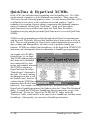
QuickTime & HyperCard XCMD's..........................................................3-10
Database Access.....................................................................................3-14
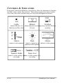
C HAPTER 4 INSTRUMENT D ESIGN
In the future, programmers will not program...........................................4-1
SoundScope Objects ...............................................................................4-2
Waves ..................................................................................................4-3
Displays................................................................................................4-4
Journals................................................................................................4-5
Controls & Indicators ............................................................................4-6
Markers................................................................................................4-7
Menubars..............................................................................................4-7
Tasks....................................................................................................4-8
Instructions...........................................................................................4-8
Datapipes..............................................................................................4-8
Variables ..............................................................................................4-9
Strings..................................................................................................4-9
Tasks and Instructions............................................................................4-10
Functions..............................................................................................4-20
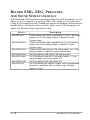
Record EMG, EEG, Pressures & Sound...................................................4-24
QuickTime............................................................................................4-25
Instruments
Glottal Video ........................................................................................4-25
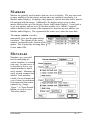
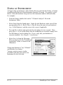
C HAPTER 5 INSTRUMENTS
Using an Instrument...............................................................................5-2
Object Naming Conventions....................................................................5-3
SoundScope Instruments.........................................................................5-4
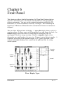
C HAPTER 6 FRONT P ANEL
Display Types .......................................................................................6-1
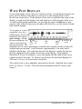
Wave Plot Displays................................................................................6-2
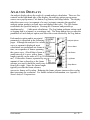
Analysis Displays...................................................................................6-3
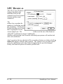
Spectrogram.....................................................................................6-4
LPC History .....................................................................................6-7
HS Slice ...........................................................................................6-9
Average Spectrum.............................................................................6-10
Fundamental Frequency.....................................................................6-12
Jitter................................................................................................6-14
Shimmer ..........................................................................................6-15
HNR ................................................................................................6-16
Envelope..........................................................................................6-17
Energy.............................................................................................6-18
Zero Crossing...................................................................................6-19
Spline ..............................................................................................6-20
LPC Residual.................................................................................... 6-21
Snapshot Displays ..................................................................................6-22
Time Interval ...................................................................................6-23
Wideband and Narrowband FFT.........................................................6-24
LPC.................................................................................................6-26
Cepstrum .........................................................................................6-27
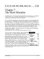
C HAPTER 7 SHORT M ENUBAR
Overview..............................................................................................7-1
Menus ..................................................................................................7-1
File menu.........................................................................................7-2
Edit menu ........................................................................................7-5
Sound menu......................................................................................7-7
Wave menu ......................................................................................7-11
Display menu.................................................................................... 7-18
Journal menu....................................................................................7-20
Task menu........................................................................................7-21
SoundScope User's Manual
A PPENDIX A SOUND A NALYSIS C OMPUTATIONS
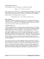
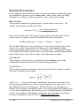
The Fourier Transform..........................................................................A-1
Basic Definitions ..................................................................................A-5
The FFT ..........................................................................................A-5
The Inverse FFT...............................................................................A-5
The Hamming Window .....................................................................A-6
Zero Padding....................................................................................A-6
6 dB Pre-Emphasis............................................................................ A-6
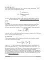
Algorithms and Formulas.......................................................................A-7
Average Spectrum.............................................................................A-7
Cepstrum .........................................................................................A-7
Energy.............................................................................................A-8
Envelope..........................................................................................A-8
FFT.................................................................................................A-8
Fundamental Frequency (F0) ..............................................................A-8
Harmonic-to-Noise Ratio (HNR).........................................................A-9
Horizontal Spectral Slice (HS Slice).....................................................A-10
Jitter................................................................................................A-10
Linear Predictive Coding (LPC).........................................................A-11
LPC History .....................................................................................A-12
LPC Residual.................................................................................... A-13
Shimmer ..........................................................................................A-13
Spectrogram.....................................................................................A-13
Spline ..............................................................................................A-14
Zero Crossing...................................................................................A-15
Sound Statistics..................................................................................... A-16
Breathiness.......................................................................................A-16
F0 Average .......................................................................................A-16
F0 Kurtosis .......................................................................................A-16
F0 Perturbation .................................................................................A-17
F 0 Range...........................................................................................A-17
F0 Skewness ......................................................................................A-17
F0 Standard Deviation ........................................................................A-18
Harmonic-to-Noise Ratio (HNR).........................................................A-18
Shimmer ..........................................................................................A-18
Voiced, Unvoiced and Silent...............................................................A-18
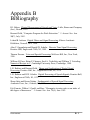
A PPENDIX B BIBLIOGRAPHY
A PPENDIX C TIPS
Instruments
Chapter 1
Installation
Welcome to the wonderful world of SoundScope. We are extremely excited about
this product and hope you can share in our enthusiasm. SoundScope is more than
just 1 product, it is a core technology on which the following products are based:
SoundScope/16
SoundScope/LC
SoundScope/8
SoundScope/16 Open
Base Package
Novice Level System
Entry Level System
C Programmer's Dream
#GWI-SoS16
#GWI-Sos/LC
#GWI-SoS8
#GWI-Sos-C
SoundScope software fully supports the MacSpeech Lab I and II hardware for
record, play and analysis. GWI is committed to the SoundScope platform and will
continue to develop it throughout this decade and into the 21st Century.
T O G ET STARTED
To get started, we recommend that you first Install the software and take a tour with
Chapter 2, Tutorial. To learn about advanced features, please see Chapter 3,
Advanced Tutorial, and Chapter 4, Instrument Design.
If you are working with a demonstration version of the software and want more
information, please contact GW Instruments and order a copy of the SoundScope &
SuperScope II Reference Manual, order #GWI-Demo-SS2-Ref. If you are interested
in adding your own C source code to SoundScope and want more information, please
order the SoundScope Open Programmer's Guide and ThinkC Interface Source
Code, order #GWI-Demo-SS2-C.
Instruments
1 - 1
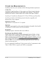
COMPUTER REQUIREMENTS
SoundScope must be run on a machine with the following minimum requirements:
COMPUTER
SoundScope/16 and SoundScope/16 Open requires one Nubus slot and is therefore
compatible with Macintosh II series and Quadra series computers. Note that the
Macintosh IIsi requires a NuBus adapter card, available from Apple Computer.
SoundScope LC installs into a Macintosh LC, LCII or LCIII Processor Direct Slot.
SoundScope/8 attaches to the Modem port and is therefore compatible with
Macintosh SE or later computers.
O PERATING SYSTEM
Apple System 7.x or System ≥6.0.7 is required.
MONITOR
Although it is not required, a color or grayscale monitor and graphics board capable
of displaying 256 shades produces the best spectrograms.
H ARD D ISK
SoundScope requires a hard disk with at least 6 MB free.
R ANDOM A CCESS M EMORY (RAM)
At least 4MB of RAM is required when running under System 6 Finder. At least
5MB is required when running under System 6 MultiFinder or System 7.0. More
RAM is needed if your System Folder contains many extensions ("INITs"), or if you
wish to record long utterances. In summary, 8MB of RAM is recommended. If you
incur a memory error upon application launch, try setting the Memory Allocation
field to 2.5MB or so (i.e. select the SoundScope application from the Finder and
choose Get Info under File).
If you are running the SoundScope/16 Open system (used by C programmers) under
Think C, 8MB of RAM is required, and 16MB is recommended.
1 - 2
SoundScope User's Manual
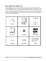
SYSTEM COMPONENTS
The SoundScope product family includes the following systems:
BASIC PACKAGE
#GWI-SoS16
S OUND S COPE /16
◊ SoundScope/16 Software on floppy disk
◊ SoundScope User's Manual and SoundScope & SuperScope II Ref. Manual
◊ AudioMedia™ II 16-bit digitizer board, cables, AudioMedia software, and
AudioMedia manuals. Technical support on AudioMedia products is available
directly from Digidesign.
◊ RANE Microphone Amplifier and cables
◊ BOSE™ powered speakers and cables
◊ Microphone, cable and stand
◊ Eve™ security key
SOUND SCOPE /LC
Novice Level System
#GWI-SoS/LC
◊ SoundScope/16 Software on floppy disk
◊ SoundScope User's Manual and SoundScope & SuperScope II Ref. Manual
◊ AudioMedia™ II 16-bit digitizer board for Macintosh LC, cables, AudioMedia
software, and AudioMedia manuals. Technical support on AudioMedia products
is available directly from Digidesign.
◊ RANE Microphone Amplifier and cables
◊ BOSE™ powered speakers and cables
◊ Microphone, cable and stand
◊ Eve™ security key
S OUND S COPE /8
Entry Level System
#GWI-SoS8
◊ SoundScope/8 Software on floppy disk. SoundScope/8 software is identical to
SoundScope/16 software, except: it does not play/record to/from the 16bit
digitizer board, it loads 16bit sound files with a maximum resolution of 12bits, it
digitizes via the Sound Control Panel with a maximum resolution of 8bits, and it
does not run Tasks.
◊ SoundScope User's Manual and SoundScope & SuperScope II Ref. Manual
MacRecorder™ 8-bit digitizing microphone, MacRecorder software, and
MacRecorder Manuals. Technical support on MacRecorder products is available
directly from MacroMedia.
S OUND S COPE /16 OPEN
C Programmer's Dream
#GWI-SoS-C
◊ SoundScope/16, described above
◊ ≥40MB External Hard Disk
◊ SoundScope ThinkC Object Code & ThinkC Interface Source Code
◊ SoundScope Open Programmer's Documentation
Instruments
1 - 3
S OUND S COPE /8 FIVE -P ACK
Multiple Systems
#GWI-SoS8-5x
◊ Five additional copies of SoundScope/8 for a multi-station installation. At least
one base system (e.g. Part #GWI-SoS8) must be purchased in order to qualify for
the Five-Pack purchase. Five-Packs cannot be broken (e.g. you cannot buy 3 for
60% of the Five-Pack price).
S OUND S COPE /16 FIVE -P ACK
Multiple Systems
#GWI-SoS16-5x
◊ SoundScope/16, described above
◊ Four additional SoundScope/16 security keys for a multi-station installation. At
least one base system (e.g. Part #GWI-SoS16) must be purchased in order to
qualify for the Five-Pack purchase. Five-Packs cannot be broken (e.g. you
cannot buy 3 for 60% of the Five-Pack price).
1 - 4
SoundScope User's Manual
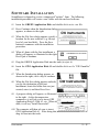
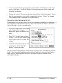
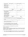
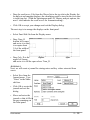
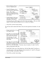
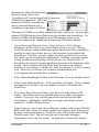
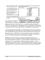
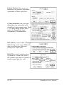
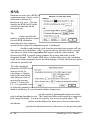
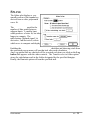
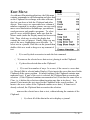
SOFTWARE INSTALLATION
SoundScope is shipped to you in a compressed "archive" form. The following
installation procedure will create a new folder with the enclosed software.
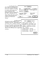
#1 Insert the GREEN Application Disk and double-click on its .sea file.
#2 Press Continue when the Introduction dialog
appears, as shown to the right.
#3 When the File Save dialog appears, specify a
location for the new software (e.g. the top
level of your hard disk). Press the Save
button to commence with the installation
procedure.
#4 When it's done with the first installment, a
dialog will appear, as illustrated to the right.
Press Quit to continue.
#5 Drag the GREEN Application Disk into the trash (to eject it).
#6 Insert the GWI Application Disk #1 and double-click on it's "GWI Installer"
file.
#7 When the Introduction dialog appears, as
shown to the right, click a key to continue.
#8 When the File Save dialog appears and asks
you for the destination of the next
installment; locate the folder that was just
created, enter it, and then Press Save.
#9 A progress dialog will appear, as illustrated
to the right. As the decompression
commences, it will ask you to insert GWI
Application Disk #2, Disk #3, etc. When it's
done, it will say "Install Successful".
#10 The computer will then ask you to insert
GWI Application Disk #1. After doing this,
drag its icon into the trash.
Instruments
1 - 5
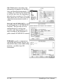
#11 L ARGE -SCREEN M ONITORS
If you are using a monitor that is 16" or greater (measured along the diagonal),
SoundScope may run out of memory when computing large spectrogram or
LPC history plots. You can prevent this problem by allocating additional
memory for SoundScope, as explained below.
• Locate the "SoundScope/xx" or "GWI Application" file in the "SoundScope
Application" folder (where xx is 8, 16, or Demo). Click the icon once to
select it, and then choose Get Info under the File menu.
• In the lower right corner, type in the number “4000” (or larger). This
number is the maximum amount of memory (in bytes) that the application
will be able to use while it is running.
• Click the close box in the upper left corner.
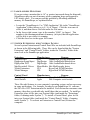
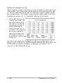
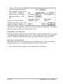
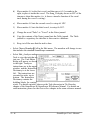
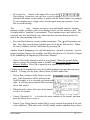
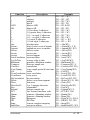
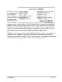
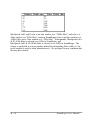
#12 S YSTEM E XTENSIONS A ND C ONTROL P ANELS
Several system Extension and Control Panel files are included with SoundScope
as shown in the following table. These files can be found within the "System
Extensions" and "Control Panels" folders, inside the "Goodies" folder at the
same level as the SoundScope application.
Extension
SSProtect INIT
Digidesign Sound Input
DigiSystem INIT
MacRecorder® Driver
XLink Extensions
XLink Manager
Manufacturer
Purpose
GWI
SoundScope/16 copy protection
DigiDesign 16bit AudioMedia board driver
DigiDesign 16bit AudioMedia board driver
MacroMedia 8bit MacRecorder driver
CEL
HyperCard XCMD Interface
CEL
HyperCard XCMD Interface
Control Panel
XLink Setup
Serial Switch
Manufacturer
Purpose
CEL
HyperCard XCMD Interface
Apple
Fast Computer serial switch
These files add features to your computer's operating system, and are necessary
in some applications. For example, in order to run SoundScope/16 software,
the SSProtect INIT Extension must be installed. Each Extension consumes some
memory; therefore you should only install those that are needed. To install an
Extension, place its file into your System folder (and inside the "Extensions"
folder, if running under System 7). To install a Control Panel, place its file
into your System folder (and inside the "Control Panels" folder, if running
under System 7). To activate an Extension or Control Panel, Restart the
computer.
1 - 6
SoundScope User's Manual
• If you have SoundScope/LC, SoundScope/16, or SoundScope/16 Open, install
the SSProtect INIT Extension.
• If you have a 16bit SoundScope/16 or SoundScope/LC digitizer board, install
the Digidesign Sound Input and DigiSystem INIT Extensions.
• If you working with the demonstration version of SoundScope, please install
the following Extensions: XLink Extensions, XLink Manager. Also install
the XLink Setup Control Panel.
• If you have a SoundScope/8 8bit digitizer, install the MacRecorder® Driver
Extension.
• If you want to run HyperCard XCMDs (e.g. in the TriVowelgram
instrument), install the XLink Extensions and XLink Manager Extensions;
and then install the XLink Setup Control Panel.
• If you want to run an 8bit digitizer, or a MacSpeech Lab I digitizer with a
Macintosh IIfx or Quadra computer, install the Serial Switch Control Panel,
double-click on it, and then choose Compatible.
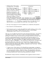
#13 SECURITY K EY
In order to run SoundScope/LC, SoundScope/16 or
SoundScope/16 Open, the Eve security hardware
key must be attached to your Macintosh. Locate
the key (a small gray box with a short cable) and
plug the key into any available Apple Desktop Bus (ADB) port. Most
Macintosh computers have 2 ADB ports on the back of the computer, and two
on the keyboard. ADB devices can be "daisy-chained", such as plugging the
mouse into the Eve security key, which is in turn plugged into the keyboard.
SoundScope/8 does not require this key.
#14 Restart your computer to activate the Extensions and Control Panels, if you
have not already done so.
#15 Double-click on the "GWI Application" file (in the recently installed folder).
Please insert the GREEN Application Disk when requested. After the
application appears with an empty front panel, it will ask you to exit (to reset
the desktop) and re-enter by double-clicking on the application file.
#16 Create a new folder outside the SuperScope II application folder and label it
"SS2 Instruments & Data". Please keep your personal instrument and data files
in this folder, separate from the SuperScope II files, to reduce the chance of
deleting an important file during a software update.
You have now completed the installation procedure -- congratulations! If you
want a tour of the software, please proceed to Chapter 2, Tutorial.
Instruments
1 - 7
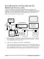
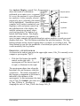
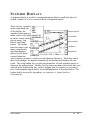
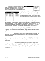
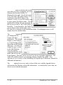
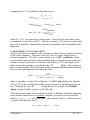
S OUND S COPE /16 AND S OUND S COPE /LC
H ARDWARE INSTALLATION
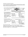
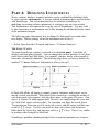
This section describes how to install the SoundScope/16 and SoundScope/LC
hardware, as illustrated in the following figure. The recommended wiring is not
mandatory since the AudioMedia II board can attach to any standard audio source or
input with "line-level" signals and RCA phono connectors (e.g. tape deck, CD
player, stereo amplifier, DAT tape recorder).
DAT
Recorder
AudioMedia II
Mic
in
out DIGITAL AUDIO TAPE
L
R ANALOG INPUT
L
R ANALOG OUTPUT
Power In
Line Out
Mic In
Amplifier
Macintosh
Computer
Red
Black
Red
Black
Red
Powered
Speakers
Black
Power In
#1 Before beginning, select Shutdown from the Finder's Special menu, and then
turn off the power switches for your Macintosh and all peripherals. It may be
wise to unplug the power cord as well.
#2 Locate the 16-bit digitizer board, in the AudioMedia box.
If you are installing the board into a Macintosh IIsi: make sure that you have a
Nubus Adapter Card (available from Apple Computer). Follow the instructions
in the “Installing an expansion card” section of the Getting Started With Your
Macintosh IIsi manual, then skip ahead to Step #10 Bose™ Powered speakers.
1 - 8
SoundScope User's Manual
If you are installing a SoundScope/LC board into a Macintosh LC, follow the
board installation instructions in your Macintosh LC manual, and then skip
ahead to Step #10 Bose™ Powered speakers.
#3 Remove the top cover. There are several NuBus connectors (often called
"slots") on the circuit board, aligned with removable panels (or empty holes)
along the back side. The slots are numbered according to the following scheme,
proceeding from left to right:
1 through 6
1 through 3
4 through 6
Macintosh II, IIx, IIfx
Macintosh IIcx
Macintosh IIci
#4 Choose an empty slot for your digitizer and remove the plastic or metal panel
(if any). For easy reference, write the slot number here: ___ .
#5 Touch the Macintosh power supply box (the shiny metal object in the corner) to
discharge any static electricity that your body might have accumulated.
#6 Unwrap the digitizer board, carefully handling it by the edges only.
#7 Orient the board so that the RCA phono jacks are facing the rear of the
computer and the NuBus connector on the board is aligned with the connector
on the computer.
#8 Carefully press down on the top edge of the digitizer, slowly sliding it into the
NuBus slot. If it does not insert fairly easily, take it out and try again. As you
insert the board, make sure its rear I/O panel sits well into the bracket at the
rear of the computer, and snaps into the small receptacle at the base of this
bracket. The RCA phono jacks should protrude slightly through the slot’s I/O
window at the rear of the computer.
#9 Replace the Macintosh cover. Do not power on the computer system yet.
Instruments
1 - 9
#10 B OSE™ POWERED SPEAKERS
• Unpack both speakers. The back of each speaker identifies whether it is for
the left or right channel.
• Locate the 8-foot black speaker wire (this wire is composed of two insulated
wires glued together, with exposed wire leads at each end). Notice that one
of the insulated wires bears a red stripe.
• Connect the two speakers together with the speaker wire. For both speakers,
the wire with the red stripe connects to the red receptacle, the other wire to
the black receptacle.
• Any time you plug anything into or out of these audio jacks, make sure the
computer and your audio equipment are powered off. Connect the gray
Audio Input wire from the left speaker to the two stereo outputs at the base
of the digitizer I/O panel, with the red (Right channel) plug on the bottom.
• Finally, connect the power cord from the left speaker to a power outlet.
#11 M ICROPHONE AND A MPLIFIER
• Make sure the computer and your audio equipment are powered off.
• Unpack the microphone and microphone cable.
• Insert the microphone cable’s three-prong XLR plug into the base of the
microphone, and insert the other end of the cable into the Amplifier's "Mic
Input".
• Insert the amplifier cable’s three-prong XLR plug into the Amplifier's "Line
Out" jack, and insert the other end of the cable into the Left Audio Input
connector at the digitizer's I/O panel (3rd RCA connector from top).
• Unpack the microphone stand and slide the microphone into the receptacle at
the top of the stand.
1 - 10
SoundScope User's Manual
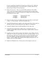
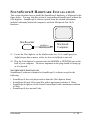
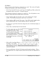
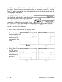
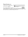
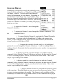
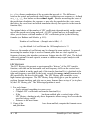
S OUND S COPE/8 HARDWARE INSTALLATION
This section describes how to install the SoundScope/8 hardware, as illustrated in the
figure below. You may skip this section if you purchased SoundScope/8 without the
8-bit digitizer. SoundScope/8 software records from the internal microphone
included with many Macintosh computers, and from MacSpeech Lab I & II
hardware.
MacRecorder
MODEM or
PRINTER port
Macintosh
Computer
#1 Locate the 8-bit digitizer, in the MacRecorder box. It is a small gray box,
slightly larger than a mouse, with a six-foot cord affixed to one end.
#2 Plug the 8-bit digitizer's connector into the MODEM or PRINTER port on the
back of your computer. The arrow imprinted on the plug should be facing up
as it is inserted.
S OUND S COPE /8 LIMITATIONS
SoundScope/8 software is identical to SoundScope/16 software except for the
following:
• SoundScope/8 does not play/record to/from the 16bit digitizer board.
• SoundScope/8 loads 16bit sound files with a maximum resolution of 12bits.
• SoundScope/8 digitizes via the Sound Control Panel with a maximum resolution
of 8bits.
• SoundScope/8 does not run Tasks.
Instruments
1 - 11
O UR M ISSION F OR T HE 90'S
The world of computing is currently evolving at lightning speed with computers the
size of notebooks doing what mainframes did only 10 years ago. And we believe
this spectacular growth will continue at a 5%/month increase in price-toperformance-ratio well into the 21st Century (it's exciting). This, coupled with the
fact that the manufacturing cost of software is negligible, has led us to believe that
companies who invest heavily in developing ultra advanced software will be the
winners at the turn of the century.
In 1989, we undertook the challenge of developing a highly advanced software
product family. This involved over 30 developers and three years of painstaking
effort before it produced it's first fruit. SoundScope is more than one computer
instrument -- it is an environment in which the end user can design their own
instruments. We believe that the next revolution in computing will involve the end
user taking on the role of the developer; designing, prototyping, learning, and
implementing new and unique methods in the field. Subsequently the SoundScope
product family allows the end user to "program" with an easy to use mouse/dialog
box user interface.
Our Company Mission is to change the way scientists, engineers and medical
researchers work in the laboratory by developing computer based instrumentation
which is faster, stronger, more accurate, more capable, more flexible, less expensive
and easier to use than the traditional benchtop counterparts. We hope this product
made a dent in this quest and wish to hear from you if you have ideas concerning
future releases.
1 - 12
SoundScope User's Manual
IDEAS F OR N EW F EATURES
If you have any suggestions for improvements, please phone or write us Attention:
New Products. We develop products for you, the user, and want your feedback.
APPLICATION NOTES
GW Instruments collects 2 page summaries of common instruments. If you would
like to write about your instrument, or would like to read about someone else's,
please call or phone GW Instruments, attention Application Note Program
Coordinator.
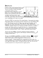
B IG B AD B UGS
To learn about dead bugs, known bugs and areas under development please open file
(choose Open under Journal) "!Development Status.c" in the "Programmer's Notes"
folder inside the "Goodies" folder. This file expects tabs every 4 characters (i.e.
choose Options under Journal and then set the Tabs to "4" characters). To report a
bug, please:
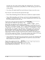
#1 If the bug causes an Error Alert to
appear (i.e. one with a Bug Report
button), press the magic button to
open the Bug Report dialog,
pictured to the right.
Alternatively, if the bug does not
cause an Error Alert to appear,
press Option 'y', at any time, to
invoke the Bug Report dialog.
#2 Read the displayed instructions.
#3 Press OK to exit the dialog.
#4 Press OK to copy the bug report information to the clipboard.
#5 Paste the clipboard text into a new word processor window.
#6 Describe the sequence of steps required to reproduce the bug (this is crucial). If
we cannot see the problem at GW Instruments, we probably cannot fix it.
#7 Delete the Dear End User letter at the top of the file, to save trees.
#8 Print in a small font and send to GW Instruments via fax, mail, or electronic
mail. If you phone us, please do so while in front of your computer, if possible.
#9 If your bug is real mean, please refer to Tip #413 in Appendix E of the
SoundScope & SuperScope II Reference Manual.
Instruments
1 - 13
IF Y OU A RE N EW T O T HE M ACINTOSH
If you are new to the Macintosh, we recommend that you keep a good reference at
your side. An outstanding one is The Macintosh Bible, 3rd Edition, by Sharon
Zardetto (Goldstein & Blair, ISBN 0-940235-11-0). Another wonderful reference is
Everything You Wanted To Know About the Mac, by Larry Hanson (Hayden, ISBN
0-672-30142-3).
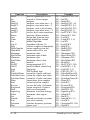
SOFTWARE U PDATES
To receive the latest version of the SoundScope software, please contact GW
Instruments. Updates are free during the first 12months, and are then a small fee to
cover shipping and handling costs. To be fair, the update fee is waived if triggered
by a software bug (i.e. it's our fault). Problems due to new computers and new
system software do not qualify as "bugs".
SoundScope/8 Software Update
SoundScope/16 Software Update
SoundScope Open Software Update
Part #GWI-SoS8-Upd
Part #GWI-SoS16-Upd
Part #GWI-SoS-C-Upd
CUSTOMER SERVICE
GW Instruments is committed to providing high-quality service to its customers.
For technical support, please contact GW Instruments by phone, fax, AppleLink,
Internet or in writing. If you phone us, please do so while in front of your
computer, if possible. Technical Support is open between 9 and 5 Eastern Standard
Time.
GW Instruments, Inc.
35 Medford Street
Somerville, MA 02143
United States
Phone: 617/625-4096
Fax: 617/625-1322
AppleLink: D 268
Internet: D [email protected]
PLEASE RETURN THE
OWNER REGISTRATION FORM
TO RECEIVE NEWS AND UPDATES.
1 - 14
SoundScope User's Manual
Instruments
1 - 15
Chapter 2
Tutorial
This chapter describes the main features of SoundScope in tutorial fashion. From
here, you can take advantage of the familiar Macintosh interface to explore
additional SoundScope capabilities.
SoundScope was created to help you record, analyze, manipulate, and play speech
and other sounds. Both recorded sounds and the result of sound calculations are
stored in the computer as waves. Specific time values in a wave may be indicated
by markers that can be moved with the mouse. The waves and markers are shown
on the screen in rectangular areas called displays. The number, size, type and
layout of displays is completely controlled by the user. There are four types of
displays, listed below.
• Wave Plot shows the timewave (voltage as a function of time).
• Analysis shows a Spectrogram, LPC History, Horizontal Spectral Slice, Longterm Average Spectrum, Fo (fundamental frequency), Jitter, Shimmer, HNR
(Harmonic-to-noise ratio), Envelope, Energy, Zero Crossing rate, Spline, or LPC
Residual.
• Snapshot shows a close-up of the timewave at a specific point in time, showing
either a 10, 20, 50 or 100 msec window, or an "instantaneous" FFT (Fast Fourier
Transform), LPC (Linear Predictive Coding) or Cepstrum.
• XY Plot shows a wave plotted against another wave (e.g. F1 vs. F2), rather than
as a function of time.
SoundScope also features integrated text editors called journals. You can type
notes directly into a journal, using it like a simple word processor. To record
numerical values, simply select the appropriate menu command and click the mouse
on specific points of interest in any wave. SoundScope can automatically pick out
peaks or other key parameters, and log them to the journal at the click of a button.
Waves, markers, displays, and journals can be combined like building blocks to
create software instruments. A few pre-defined instruments have been included
with SoundScope. You can use these as is, customize them to suit your specific
needs, or build new instruments from scratch.
In fact, SoundScope is aimed at two different audiences, instrument users and
instrument designers. Instrument users can begin work right away, using software
instruments that were created by GWI or by colleagues. Instrument designers will
Instruments
2 - 1
invest more time learning how to customize SoundScope, to create new instruments
for their own use and for use by others.
This chapter guides you through a "hands-on" interaction with SoundScope. The
Tour is divided into two chapters, each of which can be reviewed separately. In the
following instructions, each step is preceded by a bullet symbol (•). It is important
to not miss a step, since many depend on previous steps. SoundScope makes
extensive use of hierarchical menus (i.e. submenus) to provide direct access to
waves, displays, journals and other objects. This manual uses the character to
indicate a submenu. For example, "Select Load Data A from the Wave menu" is
shorthand for "Pull down the Wave menu, drag down to the Load Data submenu,
drag across to 'A', and then release the mouse button to select it."
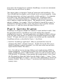
P ART 1: GETTING S TARTED
SoundScope was designed to handle two channels of sound, labelled A and B. With
the appropriate hardware, SoundScope can record and play these channels
simultaneously (in stereo). For many applications, one channel of data is sufficient.
In the first part of this tutorial, we will look at an instrument designed for a single
channel. To begin, make sure your computer is on and that you have installed the
SoundScope software, as described in Chapter 1, Installation.
• Inside the “SoundScope Application", folder on your hard disk, locate the
instrument file called "1 Channel Analyzer". Double-click on the file's icon to
launch SoundScope with this instrument. (Or, click once on the icon and select
Open from the Finder's File menu.)
Note: You will get an error message if there is not enough memory (RAM) to
launch SoundScope. As shown in it's Get Info box (select from the Finder's File
menu), SoundScope prefers 3 MB (3000 K) or more, but will run with as little as
2000 allocated. To determine if your machine has enough memory, select About
this Macintosh (or About the Finder) from the Finder's Apple () menu. If you
are running MultiFinder or System 7, quit out of other applications to increase the
memory available. Please see Chapter 1, Installation for a detailed discussion of
memory issues.
2 - 2
SoundScope User's Manual
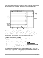
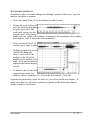
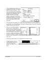
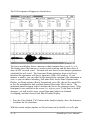
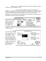
After a few seconds, SoundScope's menubar will appear at the top of the screen, and
the instrument will then be loaded. The screen will look something like this:
Marker "A1"
Marker "A2"
Snapshot
Display
"Snap_D"
Analysis
Display
"Calc_D
"
Journal
"Notes"
Wave Plot
Display
"Time_D"
Marker "A1"
Marker "A2"
Wave "A" will appear here
This instrument uses SoundScope's "Short" menubar, which provides every
command required by the typical instrument user. Additional commands for
instrument designers are available in the "Full" menubar, available from Choose
Menubar in the Edit menu. Let's begin with something tangible, recording and
playing sounds. For this tutorial, we will take them in reverse order.
L OADING S OUND D ATA FROM D ISK
To get quick results, we will start with a pre-recorded sound that was
saved to disk.
• Load a sound into channel A by selecting Load Data
A from the Wave menu.
• In the standard open file dialog that appears, select
the "were away yr ago (22.2)" file in the "Waves" folder.
This soundwave will appear in the Wave Plot display named Time_D, which runs
along the bottom of the screen. To provide unique but related names for displays and
the waves inside, display names have "_D" at the end.
Instruments
2 - 3
Wave Plot
Display
"Time_D"
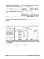
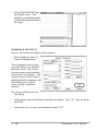
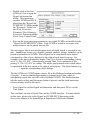
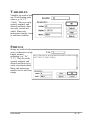
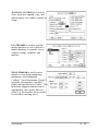
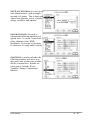
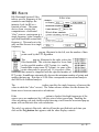
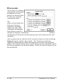
HARDWARE SETUP
In order to use the play and record commands, SoundScope must know which sound
hardware is connected to the Macintosh. SoundScope does its best to determine this
information each time it is launched; however, we will double-check to make sure
that it is correct. If you are using the demo version of SoundScope, you can play
pre-recorded sound through the speaker in your Macintosh.
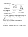
• Select Setup from the Sound
menu. A dialog will appear,
as shown to the right.
• Under the title Hardware,
make sure the pop-up menus
(Rec A, Rec B, Play A, Play
B) show the name of your
hardware: 16-Bit Digitizer,
Apple (Modem, Printer, or
Internal), MacSpeech Lab II, or MacSpeech Lab I (SoundScope/12). If you want
to play through the internal speaker, select the Internal Speaker Hardware (this is
handy if you are working with the demonstration version of the software). If
you want to record from the microphone selected in the Sound Control Panel,
select Apple with the Internal Option. If you want to record from an 8bit
MacRecorder, select Apple with the Modem or Printer Option (depending on
which port the MacRecorder is connected to).
The 16-Bit Digitizer Hardware option pertains to an AudioMedia I board, an
AudioMedia II board, or a MediaTime board. The MediaTime board (available
from RasterOps Corporation for ~$2000) includes a 24bit video circuit, a real
time frame grabber, two 16bit record channels, and two 16bit play channels -- it
is truly amazing.
• Please set the Sample Rate and Option Pop-up menus as desired. For more
information on these settings, see Chapter 6, Front Panel.
• Since you have already loaded sound data into channel A, test the hardware by
clicking on the Play A button in the lower left corner.
2 - 4
SoundScope User's Manual
• If you could clearly hear the words "We were away a year ago", then everything
is fine. If not, verify that the hardware is correctly installed, and that the
external volume control (if any) is set loud enough. If you hit "This sample rate
is not supported by your Hardware", then you can either play a sound that you
record with your hardware, or choose a wave in the "Wave" folder that is more
compatible.
• Simply click the OK button to exit the dialog box.
P LAYING A S OUND
Although sounds can be played from the Hardware Setup dialog, menu commands
(and their command-key equivalents) are usually easier.
• Select Play A from the Sound menu. You should again hear "We were away a
year ago".
You can also play just a portion of the sound.
• Click once inside Time_D (at the bottom of the screen) to make it active.
• Drag with the mouse over any portion of the wave. The selected portion will be
highlighted.
• Select Play Selected from the Sound menu.
R ECORDING A S OUND
Having chosen the appropriate hardware, you can now record a sound
to replace the current contents of the timewave. If you are using the
demo version of SoundScope, you cannot record new sounds, and
subsequently should skip ahead to Saving Sound Data on the next Page.
• Select Record A from the Sound menu. Begin speaking into the microphone
immediately after the mouse button is released. (The cursor will change into the
standard wristwatch icon when SoundScope begins to record data.) SoundScope
will record for two seconds, and then update Time_D with the new wave.
• Select Play A from the Sound menu. If the sound is too soft, try holding the
microphone closer to your mouth and recording again. (If you have
SoundScope/8, SoundScope/12, or the MacSpeech Lab I or II hardware, adjust the
hardware volume control and record again.)
Instruments
2 - 5
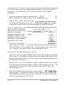
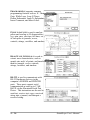
• Select Controls from the
Sound menu. Change the
length of recording to one
second by typing "1" into the
Duration text box.
• Exit the dialog and record a
new sound 1 second in
duration.
S AVING S OUND D ATA
Before proceeding, save this
sound to a new file.
• Select Save As A from the
Wave menu.
• Type "first wave" into the standard file dialog, and click on the Save button. You
may have noticed that the files names of the supplied waves are suffixed with the
sample rate (e.g. "(22.1)" means 22.1Ksamples/sec). This helps distinguish wave
files from instrument files and is useful when working with different sample
rates.
SAVING THE H ARDWARE SETUP
To preserve changes in the hardware setup, save the instrument to disk.
• Select Save As from the File menu.
• Type "my 1 Ch Analyzer" into the standard file dialog, and click on the Save
button.
That concludes Part 1 of the tour. Stay tuned for a review of all displays that are on
the screen.
2 - 6
SoundScope User's Manual
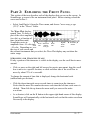
P ART 2: EXPLORING
THE
F RONT P ANEL
This section of the tour describes each of the displays that you see on the screen. In
SoundScope, a screen is like an instrument front panel. Before starting, reload the
wave used in Part 1.
• Select Load Data A from the Wave menu, and choose "were away yr ago
(22.2)" in the "Waves" folder.
The Wave Plot display,
named Time_D, shows a
plot of the wave amplitude
(in volts) as a function of
time (in milliseconds).
Sound data varies in
Timescale
Right
Scroll Wave Plot
Scroll
Left
Arrows
Scroll
amplitude from -10 volts toScroll
Box
Display
Bar
Arrow
"Time_D"
+10 volts. Depending on Arrow
the size of your screen and
the software instrument that you select, the Wave Plot display may not show the
entire range.
S CROLLING AND C HANGING S CALE
If only a portion of the timewave is visible in the display, use the scroll bar to move
around:
• Click or press on the right and left arrows for precise movement, drag the scroll
box to move to a specific location, or click on either side of the scroll box to
move by about 75% of a screenful.
To change the amount of time that is displayed, change the horizontal scale
(milliseconds per division):
• Click the down timescale arrow several times to zoom in on the timewave.
Notice that the msec/Div number decreases each time the left time scale arrow is
clicked. Then click the up timescale arrow until you can see the entire
waveform.
• As a shortcut, click on the H button in the upper right hand corner of this display.
SoundScope will automatically set the horizontal scale so that the entire waveform
fits exactly in the display.
Instruments
2 - 7
M OVING M ARKERS
Specific time values in a wave may be indicated by markers that can be moved with
the mouse. Two markers, A1 and A2, are currently visible in both Time_D and
Calc_D above it. Each marker can be moved independently of the other, and will
stay put until it is moved again.
• Click once inside Time_D (at the bottom of the screen) to make it active.
• Move the mouse pointer to the left-most marker, A1. When the mouse pointer
lies directly on the marker, hold down the Option key (which changes the cursor
to
), press the mouse button and drag the marker about half an inch in either
direction. Release the Option key and the mouse button. If you have trouble
moving the marker, make sure you are placing the cursor exactly on top of the
marker in Time_D. Then press the mouse button and hold it down as you move
the mouse to the right or left.
T HE M ARKER L ABEL A REA
The row of text and numbers at the top of Calc_D is called the marker label area,
and shows information pertaining to marker positions. In this instrument, the
marker names and time positions within the wave (in seconds) are shown directly
above each marker. The time difference is also shown, on the far left side of the
marker label area.
• In Time_D, move markers A1 and A2 in turn and notice how the numbers in the
marker label area reflect the positions of the markers.
Because the SoundScope front panel is completely customizable, an instrument
designer could show a marker label line directly above Time_D instead of or in
addition to the one above Calc_D.
2 - 8
SoundScope User's Manual
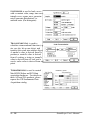
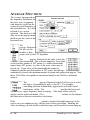
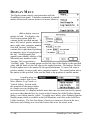
Our Analysis Display, named Calc_D,
Analysis Options
shows the result of a calculation
performed on an entire wave, a segment
of a wave (the portion of a wave between
Source Wave
two markers), or the currently selected
portion of a wave (selected by the mouse;
will be highlighted). SoundScope puts a
Calc Button
complete set of analysis routines at your
fingertips, with convenient controls on
Log Button
the right-hand side of the display, the
analysis option pop-up menu, source
wave pop-up menu, Calc button, Log
Setup Button
button, and Setup button. This display
takes the source wave (or segment of a
wave) as input, computes the specified analysis option, produces a result wave and
displays that wave. The Calc button recalculates the specified analysis. The Log
button performs actions such as logging data to a journal, or executing a task. The
Setup button lets you alter the parameters of each analysis option, and select the
events invoked by the Log button.
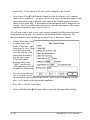
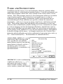
PRODUCING A SPECTROGRAM
As shown in the analysis pop-up in the upper right corner, Calc_D is currently set to
compute a spectrogram ("Spe").
• Click the Calc button (the middle
control on the right side). A
spectrogram will be drawn from left
to right, as illustrated to the right.
The spectrogram shows time along the
horizontal axis and frequency along the
vertical axis. The relative magnitude of
the frequency components at each time is
indicated by the darkness of the
spectrogram. In this instrument, the time
axis of Calc_D is linked to the time axis
in Time_D below it. Scrolling or
changing the scale of Time_D will also change Calc_D.
Instruments
2 - 9
• To see a portion of the spectrogram in greater detail, click the time scale down
arrow a few times. Scroll the display to an interesting part of the sound, and
click the Calc button.
• Change the scale to 10 msec per division and click the Calc button again. Notice
that the spectrogram is very rough, computed in discrete "blocks" or frames.
This parameter can be adjusted, as described below.
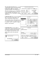
C HANGING S PECTROGRAM S ETUP
SoundScope gives you direct access to the key parameters behind each calculation. A
spectrogram is computed one frame at a time. The amount the frame is advanced
can be reduced to create a smoother plot.
• Click the Setup button on the right
side of the analysis display. A
dialog will appear as shown to the
right.
• Enter "0.5" in the Frame advance
textbox. Click the OK button in the
lower right corner to confirm this
setting.
• Click the Calc button to plot a new
spectrogram. Notice that the
display is much smoother.
The Spectrogram Setup dialog contains many pop-up menus, radio buttons and edit
fields. One especially important control that you may have noticed is the Display
range pop-up, which specifies the lower and upper frequency bounds of the
spectrogram display.
2 - 10
SoundScope User's Manual
C HANGING THE A NALYSIS O PTION
Calc_D contains many analysis options, of which the spectrogram is merely one
example.
• Select Fo Plot from the analysis pop-up menu and then Click the
Calc button. After several moments, you will see a plot of the
fundamental frequency (in Hz). Remember that the analysis display
is setup to analyze the portion of soundwave A that is visible in the
time display.
• Reset the horizontal scale by clicking the H button in the time
display, then change the analysis option back to Spectrogram. Click
Calc to see the spectrogram again.
As you may have noticed while changing back and forth between Spectrogram and
Fo Plot, many other options are available in the analysis pop-up. Each is described
in detail in Chapter 6, Front Panel.
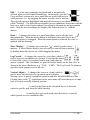
A Snapshot display
shows information
pertaining to a small
Analysis Options
interval (or frame) of
time, centered about a
Source Wave
marker. For example,
Snap_D currently shows
A1 Source Marker
a wideband FFT, which
shows the relative
Log Button
strength (in dB) of the
frequency components
Setup Button
present in the timewave
near marker A1. A
snapshot display
contains controls similar to an analysis display, with the addition of a marker pop-up
menu. Because the computations involve only a small portion of the soundwave,
they are performed immediately and no Calc button is required. The snapshot
display takes the source wave as input, computes the specified snapshot option for the
frame centered about the source marker, produces a result wave and displays that
wave. Each time one of these items changes, the display automatically recalculates
and displays the new result. The Log button performs actions such as logging data
to a journal, or executing a task. The Setup button lets you alter the parameters of
each analysis option, and select the events invoked by the Log button.
Instruments
2 - 11
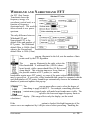
C HANGING THE S NAPSHOT O PTION
Wideband FFT is one of several options available. For information on all options,
please see Chapter 6.
• In Snap_D, select Narrowband FFT from the options pop-up menu. The plot will
resemble the wideband FFT, but with rougher, more jagged features.
• Click once inside Time_D to make it active.
• Move marker A1 a few times in the time display to get a feel for the narrowband
FFT plot. Then go to the options pop-up menu again and select Wideband FFT to
return to initial option.
S NAPSHOT M ARKER L ABEL A REA
The snapshot display has its own marker and label area to identify specific values
within the snapshot result wave. In contrast, markers A1 and A2 point to values
within the original soundwave.
• Click once inside Snap_D to make it active.
• Move the marker a few times, by holding down the Option key and dragging the
mouse (press and hold the mouse button, move mouse, release button). There are
two numbers displayed at the top of the marker. The first indicates the frequency
in Hz (X axis value), the second (in parentheses) shows the magnitude in dB (Y
axis value) at that frequency.
2 - 12
SoundScope User's Manual
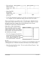
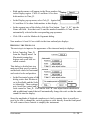
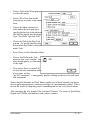
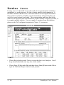
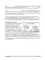
JOURNALS
SoundScope journals are simple text editors for storing key values and typing notes.
• Click once inside Time_D to make it active.
• Holding down the Option key, move marker A1 to 0.120 seconds.
• In Snap_D, click on the Setup button (the bottom of five
controls). In the dialog that appears, make sure that the
Send up to 5 peaks to journal option is checked. Click
OK to exit the dialog.
• Now click the Log button, which will send information to
the journal, as shown in the figure to the right.
Because journals are text editors, it is easy to reformat the
data, as shown in the illustration to the right. After selecting
a journal with the mouse, the user can easily delete, add and
rearrange text using standard Macintosh editing techniques.
You can also save journal data for use in a spreadsheet or
word processor.
• Select Save As Notes from the Journal menu.
That concludes Part 2 of the tour. The next section will cover waves, and introduce
two different software instruments.
Instruments
2 - 13
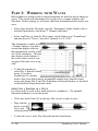
P ART 3: WORKING
WITH
W AVES
Both soundwaves and the result of sound calculations are stored in objects known as
waves. This section will demonstrate how to edit waves, compute statistics, and
filter data. Before starting, we will open a different instrument and then load a new
wave.
• Select Open from the File menu, open the "Instruments" folder (double-click or
with the Open button), and choose "1 Channel (dual time)".
• Select Load Data A from the Wave menu, switch folders up to "SoundScope"
and then down to "Waves", and select "phonetic I-A-U (10.4)".
This instrument is similar to the
1 Channel Analyzer, but adds a
second time display at the top
that automatically rescales to the
size of the soundwave. The first
time display (at the bottom of
the screen) can be used to view
any part of the time wave at any
scale.
• To hear the soundwave,
select Play A from the Sound
menu. If you have
SoundScope/16, you may
need to first select Setup (due to incompatible sample rates) from the Sound
menu, and change Play A and Play B hardware to Internal Speaker, as described
in the Hardware Setup discussion earlier.
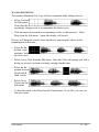
SELECTING A P ORTION OF A W AVE
It is often useful to work with a small portion of a soundwave. The standard
Macintosh technique is to use the mouse.
• Click once inside Time2_D (at the top of the screen) to make it active.
• Drag with the
mouse over the
first vowel. The
selected portion will be highlighted.
• To hear the vowel, select Play Selected from the Sound menu.
2 - 14
SoundScope User's Manual
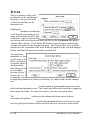
W AVEFORM EDITING
The standard Macintosh Cut, Copy & Paste commands make editing a breeze.
• Select Cut from
the Edit menu.
Notice that the
top display changes scale to accommodate the shorter wave.
• Click the mouse between the two remaining vowels, as shown above. Select
Paste from the Edit menu. Again, the display will rescale.
Next we will bring the vowels closer together by removing the silence at the
beginning and in between.
• Select the flat
portion of the
utterance, before
the first vowel.
• Select Cut or Clear from the Edit menu. Note that Clear will prompt you with a
dialog, to prevent you from accidently erasing valuable data.
• Select the flat
portion between
the second &
third vowels.
• Select Cut or
Clear from the
Edit menu.
• To hear the result, select Play from the Sound menu. If you like, you can save
this new sound.
Instruments
2 - 15
A MPLIFY AND N ORMALIZE
SoundScope lets you easily change the volume (loudness) of an entire wave, or of
any portion.
• Select Amplify A from the Wave menu. Type "50%" to reduce the volume to
half its current level. Click OK. Note that the wave amplitude drops in half in
Time_D (on the bottom). The amplitude does not appear to change in Time2_D
(on the top) because the display is set to automatically rescale in the vertical as
well as horizontal direction.
• Now select an interesting portion of the wave with the mouse, perhaps the third
vowel. Choose Normalize Selected from the Wave menu. Click OK. Note that
the wave amplitude for the selected portion increases to fill the available ± 10
volt range.
• To hear the result, select Play A from the Sound menu.
2 - 16
SoundScope User's Manual
W AVEFORM SEGMENTS
SoundScope offers a second technique for defining a portion of the wave: any two
markers can define a segment.
• Click once inside Time_D (on the bottom) to make it active.
• Change the scale to about 50
msec per division (depending
on your screen size), and
scroll until you can see the
second vowel. Note that the
markers are not visible in this display. Fortunately, the top display always shows
both markers, since it shows the entire soundwave.
• Click once inside Time2_D
(on the top) to make it active.
• Holding down the Option key
(which will change the
cursor), move one of the
markers to the left of the
middle vowel, and one to the
right. Note that the markers
appear in the bottom display
as well.
• To increase the volume of the
segment between the two
markers, choose Normalize A_S1 from the Wave menu. Click OK.
Segments are particularly useful for tasks, as you will see in the next chapter. In
many cases, however, the choice between a segment and the Selected portion is
simply a matter of preference.
Instruments
2 - 17
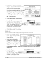
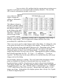
E DITING W AVEFORM V ALUES
On the computer, a sound is represented as a series of numbers or data points, often
called samples. Each sample represents the digitized voltage (typically in the range
of ±10 V) at a particular point in time. It is sometimes useful to examine and edit
the actual data values. For example, it appears that the sound volume is zero at the
beginning of segment A_S1, i.e. immediately following the left marker.
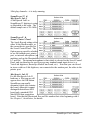
• Choose Edit Values A_S1
from the Wave menu. The
time value is shown in the
left column. Note that the
segment starts at about 0.5
seconds (depending on
exactly how much was cut
out earlier). The samples of
the wave are read left to
right, top to bottom, with
five samples on each row.
Notice that the values are not
exactly zero.
The value of any sample may be changed by typing a new number into its cell.
Ranges of cells can also be cut, copied and pasted within the table editor, and to and
from SoundScope journals and displays, or third-party spreadsheets, word
processors or other Macintosh software.
2 - 18
SoundScope User's Manual
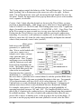
S TATISTICS & SOUND S TATISTICS
Two sets of statistics are available in SoundScope: sound statistics that are useful to
speech scientists and speech pathologists, and general waveform statistics which are
primarily intended for engineering applications.
• Click once inside Time_D (on the bottom) to make it active.
• Select a small portion (about
50 msec) of soundwave A,
from the middle of the
vowel.
• Choose Sound Statistics
Selected from the Wave
menu. The "NAN" value for
shimmer indicates that it
could not be computed. As
noted in Appendix A,
shimmer requires a longer
time interval for a good
calculation.
• From the Sound Statistics
pop-up menu at the top of the
dialog, choose A_S1. After
several seconds, you will see
the result for the entire
segment.
Note that, given the larger
amount of time as input, shimmer was successfully computed. For more
information on these statistics, see Chapter 7, Short Menubar and Appendix A,
Sound Analysis Computations. You can also compute individual statistics and save
the result to a journal or a wave, via task instructions.
Instruments
2 - 19
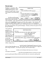
F ILTERING
Filters attenuate certain frequency components in a sound. This section will explore
filtering, and introduce a new software instrument.
• Select Open from the File menu, switch up to the SoundScope folder, and into the
Instruments folder, and choose "2 Channel Analyzer".
This instrument is designed to compare two soundwaves. We will synthesize a tone,
add noise, analyze the result, and then filter out the noise.
• Choose Synthesize A from the Wave menu. Enter 5000 into the Length
textbox. The default tone (periodic, sine) is fine, so click OK.
• Choose Synthesize B from the Wave menu. Enter 5000 into the Length textbox.
Select Uniform noise, type 1 into the adjacent volts box, and click OK.
• In order to get a good look at the data, change the scales for both time displays to
2 msec/Div.
• Choose Play A and then Play B to hear the data.
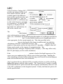
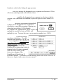
• To create a noisy tone, we will add the
two sounds (B=A+B). Choose
Calculate from the Wave menu. Press
on a few pop-ups to familiarize
yourself with this dialog. When you're
done exploring, select B = A + B from
the appropriate pop-ups, as illustrated
to the right.
• Click on Do It, and then OK.
The noise is very visible and audible (select Play B).
With SoundScope, the noise
can also be analyzed.
• For an overall picture, click the Calc buttons on both analysis displays. Where
the original tone is in a single frequency band, the noisy tone has components all
over.
2 - 20
SoundScope User's Manual
• For an instantaneous picture at a
certain point in time, use markers
and the snapshot displays. First,
move one marker into position by
selecting Move Time_D from the
Display menu, unchecking the
Display checkbox, checking
Marker, selecting To the X secs
position and typing .010 (10 msec).
Confirm that the settings match
those in the figure below, then
click OK.
• The procedure for marker B1 is easier, since the dialog uses your last choices as
the defaults: select Move Time2_D from the Display menu, choose B1 from the
Marker pop-up, and click OK.
• Make sure that both snapshot
displays show Wideband FFT. If
not, use the top control to change
from another option. In Snap_D,
move the marker to the peak of
the data, yielding the frequency of
the tone. In Snap2_D, move the
marker to the second peak, to get an idea of what frequencies we should try to
filter out.
• Click once inside Time2_D (on the bottom) to make it active.
• Using the mouse, select a
small portion of the noisy
tone that includes the
marker, say from 5 to 15
msec.
Instruments
2 - 21
• Choose Filter Selected from
the Wave menu, and change
the Frequency Cutoff for the
filter to 10% - yielding a
number close to the target
determined above. Click
OK.
Clearly, the filter worked!
Visually, the noise is gone. The
snapshot display confirms it, as
will a spectrogram. Because we
only filtered a small portion, you will not be able to hear the difference. If you like,
filter the entire soundwave B, and play the result.
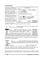
E XPLORING S OUND S COPE
Using the techniques that you have learned, please explore SoundScope on your own.
Try loading other instruments and waves. Test out any menu item or front panel
control. If you get stuck and need some help, please feel free to give us a call.
Q UITTING S OUND S COPE
The next section covers advanced features of SoundScope. If you do not want to
tackle that quite yet, you can quit and explore more at another time.
• If you do not wish to continue, select Quit from the File menu.
2 - 22
SoundScope User's Manual
P ART 4: DESIGNING INSTRUMENTS
Waves, markers, displays, journals, and tasks can be combined like building blocks
to create software instruments. A few pre-defined instruments have been included
with SoundScope. This section describes how to customize SoundScope by
modifying an existing software instrument, or creating a new one from scratch.
This information is not required for everyday user of SoundScope. You may want
to gain experience as an instrument user before learning the advanced features aimed
at the instrument designer.
The following pages demonstrate how to change the front panel layout and add a
new display. Before starting, reload the instrument used in Part 1.
• Select Open from the File menu, and choose "1 Channel Analyzer".
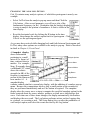
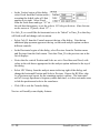
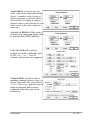
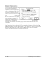
T HE F RONT P ANEL
The main SoundScope window is referred to as the front panel. It includes all
displays and front panel journals. You can change the size and position of each front
panel object with Panel Edit Mode. For example, you may want a wider journal to
enter more substantial comments. The following steps show you how to modify the
standard "1 Channel Analyzer" instrument to achieve this end.
3
2
4
1
Before
3
4
2
1
After
In Panel Edit Mode, all displays, journals, controls, indicators and pictures can be
moved, resized, and deleted. When Panel Edit is turned on, a rectangular outline of
each front panel object appears, with the object name in the upper left corner. If an
object is selected, its name appears bold. To resize, one simply drags the resize box
(i.e. little black square at lower right). To reposition, one drags the actual object.
To reposition an object one pixel at a time, one selects with the mouse, and then taps
on the
keys. To resize one pixel at a time, one selects with the mouse,
holds down the Option key, and then taps on the
keys. This is very similar
to working with rectangles in MacDraw.
SoundScope prohibits shrinking displays below a practical minimum size to ensure
Instruments
2 - 23
readable content. Individual items within a objects cannot be resized independent of
the object. Should displays or journals overlap, a warning is issued (i.e. "Invalid
Panel" in status bar) and the user is prohibited from leaving design mode until the
overlapping is eliminated.
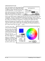
A PICT file (72 dpi picture file) can be placed
onto the front panel by first transferring it to
the clipboard (with Cut or Copy) and then
moving it to the display with the Paste
command, as illustrated to the right. Also,
PICTs can be Cut or Copied from the SoundScope front panel to the clipboard.
Since front panel displays, journals, and so forth are not PICTs, they cannot be
moved to or from the clipboard.
• Select Panel Edit On from the Display menu.
• Resize the Calc_D
analysis display and
move it down, to
make room for
rearranging other
items.
Before
After
Before
After
• Move Snap_D to
the left corner.
Then resize the
Notes journal, in
preparation for
moving it.
2 - 24
SoundScope User's Manual
• Move the Notes
journal so it is
adjacent to Snap_D.
Then move the
Calc_D analysis
display up until it
touches Snap_D.
Before
After
• Resize Calc_D to
make it taller and
occupy the full
screen width. Then
carefully resize the
Time_D wave plot
display so that the
dotted vertical lines
meet. (Tip: hold
Before
After
down the Option
key and use the right and left arrow keys to resize one pixel at a time.)
• Finally, resize the Notes journal to fill the entire
corner.
• Select Panel Edit Off from the Display menu. You
can now use the new layout.
• To save this instrument for future use, select Save
As from the File menu, type "1 Ch, wide journal"
into the standard file dialog, and click the Save button.
You have now added a new instrument to your portfolio.
A DDING A D ISPLAY
In addition to simply rearranging a front panel layout, you may want to create new
displays or journals. The following steps show you how to add a second snapshot
display to the above instrument.
• Select Choose Menubar Full from the Edit menu. New items will appear in
most of the menus (although you will not notice until you pull them down).
Instruments
2 - 25
• Snapshot (and analysis) displays
require waves to hold the result of
their calculations. To create one,
select New from the Wave menu.
• Type in the name "Snap2" and click
OK.
• Select Panel Edit On from the Display menu.
• Resize the Notes journal to make room for a new
display.
• Select New from
the Display menu.
• Type in the name
"Snap2_D", and
select Snapshot
from the pop-up
immediately below.
In the scrollable list
towards the right,
click in the gray
area (or down
arrow) of the scroll
bar to scroll down. Drag the Snap2 wave into the top slot on the right, as shown
in the diagram.
• Click OK to accept the changes and exit the dialog.
2 - 26
SoundScope User's Manual
• Move and resize
Snap2_D until it
fills the upper right
corner.
• Select Panel Edit
Off from the
Display menu. You
can now use the
new layout.
Before
After
• To save this instrument for future use, select Save As from the File menu, type "1
Ch, 2 snapshot" into the standard file dialog, and click on the Save button.
This new instrument is very similar to the "1 Ch (dual snap)", although it lacks a
fourth marker, marker label line and various custom display settings. For more
information about these settings, please see the following section, and the
SoundScope & SuperScope II Reference Manual.
C REATING A NEW INSTRUMENT
This section shows you how to create a
simple instrument with a time display,
analysis display, journal, waves, markers
and a segment. The result will look like
the illustration to the right.
• Select New Instrument from the File
menu and click OK in the confirmation
dialog. This command deletes all
waves, displays, journals, etc., allowing
you to proceed with a “clean slate.”
W AVES
This instrument will require two waves, an integer wave for holding the sound, and
a floating-point wave to hold the calculation result shown in the analysis display.
• Select New from the Wave menu. The wave options dialog will appear. Type
“A” in the Name edit box.
Instruments
2 - 27
• Sound data is stored as a series of
integers. Click the Format button and
select the 16-bit Integer option.
Waveforms recorded with 8bit, 12bit and
16bit digitizers are all stored in 16bit
integers with values ranging from -32K
to +32K (i.e. the data is packed into the
most significant bits in the case of the 8
and 12 bit digitizers).
• Click OK to exit the Format dialog.
• From the Wave pop-up menu at the
top of the wave options dialog,
select New Wave. Type the name
“Calc”. By default, waves are
stored as 32-bit floating point data,
as desired for calculation results.
• Click OK to exit the Wave dialog.
D ISPLAYS
Next we will create the displays and arrange them on the screen.
• Select New from the Display
menu. Type “Time_D” in the
Name edit box.
• Notice the two lists in the
Contents area of the dialog. The
Waves list on the left shows all
available waves and segments; the
Display list on the right shows
which waves and segments are to
be shown in our display. Drag wave A from the Waves list to any slot in the
Display list.
• From the Display
pop-up menu at the
top of the dialog,
select New Display. Type “Calc_D” in the Name edit box, and select Analysis
from the Type pop-up menu.
2 - 28
SoundScope User's Manual
• Drag the result wave Calc from the Waves list to the top slot in the Display list.
In analysis and snapshot displays, the calculation result is stored in the wave that
is in the top slot. (With the Spectrogram and LPC History analysis options, the
next 5 slots indicate the result waves for formant-tracking.).
• Click OK to accept your changes and exit the Display dialog.
The next step is to arrange the displays on the front panel.
• Select Panel Edit On from the Display menu.
• Drag Time_D
bottom left corner
and resize it so that
it occupies about
3/4 of the width of
the front panel.
• Drag Calc_D to the
Before
upper left corner
and resize it to fill the space above Time_D.
After
JOURNALS
Next, we will create a journal for storing notes and key values extracted from
waves.
• Select New from the
Journal menu. Type
“Notes” in the Name
edit box.
• Click OK to create the
journal and exit the
dialog.
• Move and resize the
journal so that it fills in
the gap remaining on
the front panel.
Instruments
2 - 29
• Select Panel Edit Off from
the Display menu. You
should see something similar
to the front panel pictured to
the right.
M ARKERS & SEGMENTS
Now we will create two markers and a segment.
• Select Markers Time_D
from the Display menu.
Take a moment to survey this
powerful dialog. It is divided
into three areas. The Display
area determines which markers
are shown in each display. The
Segment area is used to create,
modify and delete segments; and
the Marker area is used to
create, modify, and delete
markers.
We will use all three parts in
this dialog.
• In the marker area of the dialog, click the New button. Type “A1” into the Name
edit field.
• In the same way, create a second marker named “A2”.
2 - 30
SoundScope User's Manual
• Both marker names will appear in the Show markers list
in the Display region. Click A1 and then A2 to show
both markers in Time_D.
• In the Display pop-up menu, select Calc_D. Again click
A1 and then A2 to show both markers in this display.
• In the segment area of the dialog, click the New button. Type “A_S1” into the
Name edit field. Note that wave A and the marker boundaries A1 and A2 are
automatically selected in the corresponding pop-up menus.
• Click OK to exit the Markers & Segments dialog.
Now markers A1 and A2 are visible in the time and analysis displays.
R EFINING THE D ISPLAYS
The next step is to improve the appearance of the time and analysis displays.
• Select Controls Time_D
from the Display menu. In
Macintosh terminology,
buttons and scroll bars are
called controls.
This dialog is divided into two
main areas that specify controls
and default values for horizontal
and vertical scale and position.
• In the Horizontal region of the
dialog, notice that Position is
set to Scrollable and the Scale
to Adjustable. These settings
put a scroll bar control and a
scale control in Time_D. Click on the Add "H" auto adjust button checkbox to
add an additional control that will automatically change the scale so that the entire
sound fits into the display.
Since the amplitude of digitized soundwaves is fairly constant, there is usually no
need to be able to change the vertical position or scale directly from the front panel.
We will remove these controls to simplify the instrument.
Instruments
2 - 31
• In the Vertical region of the dialog,
select Fixed from the Position menu -accepting the default value of 0 that
appears to its right. Select Fixed
from the Scale menu and type “10” in
the edit box that appears, to set the scale to 10 Volts per division. (One division
on the screen is 32 pixels, about 1/2".)
For Calc_D, we would like the horizontal axis to be “linked” to Time_D so that they
will both scroll and change scale in unison.
• Select Calc_D from the Controls menu at the top of the dialog. Note that an
additional pop-up menu appears at the top, so that each analysis option can have
different controls.
• In the Horizontal region of the dialog, select Previous from the Position menu
and Previous from the Scale menu. Note that Time_D is the previous one in the
list of displays.
• Notice that the vertical Position and Scale are set to Fixed base and Fixed, with
values in the edit boxes appropriate for the analysis option indicated at the top of
the dialog.
• Select LPC History from the analysis menu in the top right of the dialog, and
change the horizontal Position and Scale to Previous. Repeat for HS Slice, skip
Avg Spectrum, and repeat for the remaining analysis options. The horizontal
axis of Average Spectrum is frequency rather than time, so it does not make sense
to link the position and scale to the soundwave.
• Click OK to exit the Controls dialog.
Next we will modify some display features.
2 - 32
SoundScope User's Manual
• Select Features Time_D
from the Display menu.
• Under Plot Region, select
None from the Grid pop-up
menu. This setting
eliminates the grid (dotted
lines at each division) in the
time display.
• In the Display Labels area,
click the Add wave labels
checkbox to de-select it,
removing the wave label region on the left of the time display. (The wave label
region is useful when more than one wave is shown in a display.)
• Click OK to exit the Features dialog.
We will also add a marker label line to show the time positions of markers A1 and
A2.
• Select Labels Calc_D from
the Display menu.
• Note that A1 is selected in the
Marker pop-up at the upper
left corner of the dialog.
Click the Show X value
checkbox below it to select
this option.
• Note that A2 is selected in the
other Marker pop-up. Click
the Show X value checkbox
below it to select this option. The time values of markers A1 and A2 will be
shown in the marker label line.
• In the Delta Values area of the dialog box, click the Show delta X checkbox to
select this option. The time difference between markers A1 and A2 will appear
on the left edge of the marker label line.
• Click OK to exit the Labels dialog.
Instruments
2 - 33
S AVING THE INSTRUMENT
Save your new instrument to disk for later use.
• Select Save As from the File menu.
• Type "my instrument" into the standard file dialog, and click on the Save button.
You may want to practice working with this instrument. Afterwards, feel free to
make additional changes to it. Also, feel free to copy and modify the instruments
included with SoundScope, or swap instruments with friends and colleagues. If you
create a special-purpose instrument, please consider sending it to us so that we can
share it with others.
W HERE TO G O FOR M ORE INFORMATION
Congratulations! You have completed the tour and are well on your way to
becoming a SoundScope expert. Chapter 3 is a detailed discussion of a sophisticated
software instrument. Chapter 4 covers the building blocks used in instrument
design. Chapter 5 describes many of the instruments that are included with
SoundScope. Chapter 6 covers the front panel, and Chapter 7 outlines all the menus
and dialogs encountered by a typical user. For background information on
computer analysis of speech, please refer to the "Manual of Clinical Applications,"
available free from GW Instruments.
SoundScope is built on top of the SuperScope II engine, and includes all features
available in the SuperScope II application program. Advanced features such as
instrument design and multi-channel data acquisition are described in the
SoundScope & SuperScope II Reference Manual.
2 - 34
SoundScope User's Manual
Instruments
2 - 35
Chapter 3
Advanced Tutorial
The dilemma in designing any product involves the tradeoff between the number of
features and ease-of-use. Products with a few features tend to be easy to learn and
use, and those packed tend to be more challenging. And in many cases, simple
applications do not satisfy the user's requirements. SoundScope overcomes the
dilemma with several features which include a menubar editing environment, a
dialog-oriented command language (referred to as "tasks"), and a powerful set of
database export tools. The Menubar Editor enables an instrument designer to create
a menubar, and assign tasks to each menu item. The menubar can contain any
number of menus and commands; subsequently making it possible to create a very
simple instrument, with only a few commands (e.g. Record, Analyze, Print, Save
Data, Export To Database). And hence, the user can have it both ways with
SoundScope: simple and easy, or featureful and complicated. An example is the
Professor who wants a powerful environment for himself/herself, yet who wants a
very simple environment for his/her students.
This chapter provides a tour of a simple instrument that records three vowels,
analyzes them, and sends the results to a FileMaker database. The name of the
instrument is "TriVowelgram™", and it is described in detail in Chapter 5,
Instruments. The following discussion will show the reader how to create tasks and
menubars, and how to interface SoundScope to another application program. It is
not necessary to understand these features in order to use SoundScope; they are only
used by the Instrument Designer, as opposed to the Instrument User. So, if you want
to learn about instrument design, please proceed. Please note that SoundScope/8
does not run Tasks, and therefore will not support several of the instructions in this
chapter.
• Please exit SoundScope, find the TriVowelgram™ instrument, select it, and
choose Duplicate under File. This will cause the file to be duplicated and
renamed to "TriVowelgram™ copy". It is good to work with a copy of an
instrument when doing design; so you can return to the starting point, if desired.
Also, as you are designing, it is always good to save your instrument every now
and then with an different file name (e.g. fred1, fred2, fred3, etc), to protect
against the unexpected.
• Double-click on TriVowelgram™ copy; or launch SoundScope, and then choose
Open under File to load the instrument.
Instruments
3 - 1
The TriVowelgram will appear as shown below.
The lower most display shows a timewave which contains three vowels (e, o, u).
The display above the timewave is used for pitch tracking, and the three above it
show an LPC for each vowel. The main text area shows several analysis parameters
calculated for each vowel. The front panel Sizing option has been set to Fixed;
therefore this instrument will always open into a 640 x 480 window. If your
monitor is smaller, you can either do the tutorial with a portion of the instrument in
view, or you can choose Menubar Full under Edit, choose Panel Options under
Display, set Sizing option to Resize Proportional, press OK, choose Save under File
to save the instrument to disk, and then choose Open under File to load it. The
instrument should reappear with it's window the size as the computer screen. If the
front panel is too crowded on the screen (i.e. it gives you a "Front Panel is Invalid"
message), you will need to resize several front panel objects to eliminate
overlapping, and then choose Panel Edit Off under Display.
• Press the Calc (labeled "Cal") button in the Analysis display, above the timewave,
to initiate the Fo calculation.
With the current analysis options, an Fo track may not be feasible (i.e an Fo plot
3 - 2
SoundScope User's Manual
does not appear).
• Choose Options under Calculate (or press Option 'l' {lower-case letter L}) to
open the Analysis Options dialog, and then set the acceptable pitch periods to
150Hz to 210Hz. Press Ok to exit the dialog, and then press the Calc button
again. A valid pitch track should appear, as shown below.
Pitch tracking is more of an art
than a science, and it is often
necessary to adjust the pitch
track options before proceeding
with pitch-based analysis such as HNR, shimmer and jitter. In other words, don't
trust the TriVowelgram's data if a good pitch track could not be attained. In the
above example, the second vowel is a little clipped at the ±10V bound, causing it's
Fo plot to waiver. Consequently, the HNR value calculated from this vowel is
NAN(021), which means "not a number" (i.e. it could not be determined). We
include this case intentionally to make the reader more aware of issues that appear in
the field.
• Choose Complete Analysis in the Calculate menu. This will cause the Analysis
Task to run, which does the following:
a)
Clear the main journal, above the 3 LPC displays.
"Voiced"
b)
Calculate the voiced intervals of the timewave, and place
the result into a wave called "Voiced". The points in this
wave are set to 1.0 where the timewave is voiced, and 0.0
elsewhere. It is plotted above the timewave, as shown in the illustration to
the right.
c)
Do the following three times:
A) Find the first pulse in the Voiced wave. Notice that a pulse in Voiced
corresponds to a voiced interval, which should be a vowel. Markers A1
and A2 are moved to the beginning and end, respectively, of the voiced
interval. Segment A_S1 is defined in the Marker dialog as the part of
the timewave (referred to as "A") between markers A1 and A2, and
should therefore contain a vowel.
B) Calculate sound statistics on segment A_S1 (i.e. the vowel). Shimmer,
HNR, breathiness, jitter, Fo average, and Fo range values are sent to
journal Notes, and appear as one row in the table.
Instruments
3 - 3
d)
Move marker A1 to the first vowel, and then move it 0.1 seconds to the
right, to place it inside the vowel. The Snap_D display shows an LPC of the
timewave about this marker (i.e. it shows a transfer function of the vocal
track during the vowel's voicing).
e)
Move marker A2 into the second vowel, to setup it's LPC.
f)
Move marker A3 into the third vowel, to setup it's LPC.
g)
Change the word "Pulse" to "Vowel" in the Notes journal.
h)
Copy the contents of the Notes journal into the Table journal. The Table
journal is a repository for data that is later sent to a database.
i)
Beep, to tell the user that the task is done.
• Select Choose Menubar Full in the Edit menu. The menubar will change to one
that includes the standard SoundScope commands.
• Select Edit Analyze under
Task to view the task that we
just ran. The Task Editor
dialog will appear, as shown
to the right. Analyzes
instructions are in the upper
window, and the Instruction
Dictionary is at the lower
left. The instructions are
executed in order, top to
bottom. The Instruction
Dictionary contains the
building blocks for creating
a task. For details on tasks, please see the Task discussion in The Menubar
chapter of the SoundScope & SuperScope II Reference Manual. For details on
each instruction, please see the Instructions chapter in the same reference manual.
3 - 4
SoundScope User's Manual
• Double-click on the Voiced =
Voiced(A) line. A Calculate
Wave dialog will appear, as
shown to the right. This dialog is
used to execute one of the 80
functions and operators. For
details on each, please see the
Functions and Operators chapter
in the SoundScope & SuperScope
II Reference Manual. Pop-up
menus and radio buttons are used
to setup a calculation. Each popup contains a list of waves, a list of functions (e.g. cos(), FFT()), or a list of
operators (e.g. +, - ,*). The dialog is currently setup to calculate the Voiced
interval of the A wave and place the results into a wave named Voiced.
• Press on a few pop-ups to view the available waves, functions and operators.
• Press Cancel to exit the instruction.
• Each instruction can be viewed and modified by double-clicking on the text that
appears in the task region. Double-click on a few to see their dialogs,
remembering to press Cancel to exit each instruction.
There are over 20 different instructions in the Instruction Dictionary, each with it's
own dialog environment. One views or edits an existing instruction by doubleclicking on it and one copies an instruction by selecting it and then choosing Copy.
To paste a copied instruction into a task, install a task insertion pointer (i.e. a
horizontal dotted line) by clicking on the instruction above your target, and then
choose Paste. The copied instruction will appear immediately after the selected
instruction (which is highlighted). One can Delete an instruction by selecting it and
pressing the Delete key, and create a new instruction by dragging it from the
Instruction Dictionary into the task region. Tasks can be created, deleted, edited,
and run with the New, Delete, Edit, and Run commands in the Task menu. And this
is how one "programs" SoundScope.
• To gain a sense of the richness of the SoundScope programming environment,
double-click on each instruction in the Instruction Dictionary, pressing Cancel to
exit each instruction's dialog. Double-clicking is like dragging the instruction
from the Dictionary to the end of the task. Pressing OK causes the instruction to
be inserted into the task, Cancel causes the insertion to be aborted.
Recall that the Analyze task bases calculations on the segment of timewave that is
Instruments
3 - 5
considered voiced. Fo tends to vary a little at voicing onset and offset; subsequently,
it is desirable to move the two segment-defining markers, A1 and A2, inward, to
eliminate the onset-offset effects. We will do this with two Move Marker
instructions.
• Scroll the Instruction Dictionary until the Move
Marker Instruction is visible, as shown to the right.
• Drag the Move Marker instruction from
the Instruction Dictionary into the task
area and put it under the Pulse analysis instruction, as shown to the right.
The Move Marker dialog will
appear, as shown to the right.
This instruction is used to move
markers to waveform
minimums, maximums, local
minimums ("valleys"), local
maximums ("peaks"), upstrokes,
downstrokes, specified points,
and specified wave values.
• Set the Move to pop-up to
relative time X, set the X
offset edit field to +0.050, and press OK. This instruction is now setup to move
the A1 marker to the right by 50ms, before analyzing the vowel.
Now lets move the right edge marker to the left.
• Click once on your new Move Marker instruction to select it, choose Copy under
Edit to copy it to the clipboard, and then choose Paste under Edit to paste it into
the task, at the position of the dotted line, which is conveniently right before the
Sound Statistics instruction.
• Double-click on your new instruction, to open it's dialog, and then select marker
A2 in the upper-most pop-up, change +0.050 to -0.050, and then press OK. This
instruction is now setup to move the A2 marker to the left by 50ms, before
analyzing the vowel.
• Press the Go button at the upper right to run the task in
debugger mode. A triangle will appear at the left ( ) that
shows which instruction is being executed. After a few seconds, press the Step
button to temporarily halt the execution.
3 - 6
SoundScope User's Manual
• Now press the W button, at the upper-left, to open the
Wave dialog. From here, one can view a wave's values
with the Edit button, or the number of points with the Points button, for example.
To view another wave, simply select it in the upper-most pop-up menu. Press
OK to exit this dialog.
The C, J, M, S, V and W buttons are used to view and modify controls, journals,
markers, strings, variables, and waves; during, before, or after running a task. This
is helpful when a "problem" is encountered. These buttons cause a new object to be
created if one does not already exist; otherwise they open the dialog for the first
item in the corresponding object list.
• Press the Step button to execute another instruction. The ( ) will increment one
line. Press Step several times, and then press Go to let the task run free. When
the task is finished, exit the Task Editor by pressing OK.
Another form of debugging is to send information to a journal at run time. Several
journal reporting features are available, and fully described in The Menubar Chapter
of the SoundScope & SuperScope II Reference Manual.
• Choose New under Journal to create a new journal. When the journal dialog
appears, change the journal's name to Task80; and then set the Position pop-up
menu to Window. Press OK to open the new window-based journal.
Clicking in the front panel will cause the Task80 journal to become the back-most
window. To bring it to the front, choose Show Task80 under Edit.
• Choose Run Analyze under Task to run the
task. Each instruction will be written to the
Task80 journal, as it is executed; as shown to the
right. It will beep when finished (this task may
take a little while).
• When the task is done, click once in the journal
to select it's window.
• Choose Cloverleaf 'a' ( a) to select the entire contents of the journal, and then
press the Delete key to erase it.
• Choose Copy Task Analyze under Edit to copy a textural description of the task
to the clipboard. Click once in the Task80 journal window and then choose Paste
Instruments
3 - 7
under Edit. A description of the task will be dumped to the journal.
• Now choose Clear Task80 under Journal to clear the journal of it's contents
(notice this is similar to a), press Option 'a' to copy a textual description of the
entire instrument to the clipboard, click once in the Task80 journal, and then
choose Paste under Edit. A description of the instrument will be dumped to the
journal. Use the scrollbar and resize box to view this description. For a more
complete description, press Option Shift 'A'.
We will now create a task, create a new menu command, and then setup the menu
command to run the task. For details on the Menubar Editor, please see The
Menubar chapter in the SoundScope & SuperScope II Reference Manual.
• Choose New under Task
to create a new task.
Name it "myTask", and
then drag the Alert, Beep
or Delay instruction
(near the bottom of the
instruction dictionary)
into the task region.
Select the Display
message radio, enter
"Hello." into the edit
field, and then press OK
to install the instruction.
• Press Go to see the task
run. It should execute
the instruction which produces the "Hello," alert. Press Continue to exit this
alert. In Go mode, tasks beep upon completion.
• Press OK to exit the Task Editor.
• Choose Edit Menubar Full under Edit to open the Menubar Editor dialog.
3 - 8
SoundScope User's Manual
• Choose Task in the Menu pop-up
to select this menu.
• Choose New User Item in the
Item pop-up to create a new menu
item.
• Choose the Show custom text
radio under the item pop-up to
specify that the text in the adjacent
edit field be placed into the menu.
Type "Say Hello" into this field.
• Choose myTask in the Run Task
pop-up -- to specify that this task
be run when Say Hello is selected
under Task.
• Press Ok to exit the Menubar Editor.
• Choose Say Hello in the Task
menu to view your creation. An
alert should appear, as illustrated
to the right.
• Now choose Save As under File
to save this new instrument under
a new name, such as
"myTriVowelgram". Consequently, double-clicking on the new file will open
this instrument.
Notice that the Menubar and Task Editors enable you to build virtually any menu
driven application program, without knowledge of a programming syntax. This is
new in the world of computing, and is something that we are very excited about.
This concludes the first round of the Advanced Tutorial. For a tour of QuickTime,
HyperCard XCMDs, and database work; please continue.
Instruments
3 - 9
QuickTime & HyperCard XCMDs
In the 1970's, the world developed computing tools for handling text. The 1980's
was the decade of graphics (e.g. the Macintosh user interface). Many expect the
1990's to be the age of moving graphics (video). It is also theorized that this will be
as influential to our society as the revolutions in text and graphics. Apple's
technology for recording, playing, editing, compressing and databasing computer
videos is commonly referred to as "QuickTime". Many tools that support
QuickTime movies are available from Apple and Third Party Developers.
SoundScope can play and plot pre-made QuickTime movies via several QuickTime
XCMDs.
XCMDs are the programming port-hole through which HyperCard communicates
with the world. Physically, they are little functions whose code resides in a file on
disk. They are used primarily by HyperCard to control multimedia devices such as
tape recorders and framegrabbers, yet can be used to perform virtually any
function. XCMDs are callable from SoundScope, via the HyperCard XCMD/XCFN
instruction, and consequently add a new dimension to SoundScope programming.
An example of an XCMD is
FinderEvents, by Jon Pugh.
This XCMD sends messages to
the Finder and is distributed
non-commercially by usergroups and computer networks.
The XCMD is stored in a
HyperCard stack file called
"FinderEvents", illustrated to
the right. The stack contains
documentation on how to call
the FinderEvents() function. It
explains that the XCMD has one
parameter that tells the Finder
what to do. For example, executing FinderEvents "AboutMacintosh" from
HyperCard or SoundScope instructs the Finder to show the "About This Macintosh"
dialog. To install this XCMD into SoundScope, the user must place a copy of the
"FinderEvents" file into the "HyperCard XCMD/XFCN" folder, inside the
"Resources" folder, which must be at the same level as SoundScope, and then restart
SoundScope. Subsequently, one can create a SoundScope instruction
3 - 10
SoundScope User's Manual
that opens the About This Macintosh
dialog by typing FinderEvents
"AboutMacintosh" into the HyperCard
XCMD/XFCN instruction. XFCN are
identical to XCMD, except that they
always return information into a
SoundScope string named "retValue".
Thousands of XCMDs are available commercially and as shareware. Several Apple
authored XCMDs that play QuickTime movies are included with SoundScope. For
details on XCMDs and the SoundScope-to-XCMD interface, please see the
Instructions chapter in the SoundScope & SuperScope II Reference Manual.
• If you did not install the QuickTime, XLink Extensions, XLink Manager
Extensions; and the XLink Setup Control Panels, please do so now. Playing
QuickTime movies within SoundScope requires that the QuickTime extension be
installed in your System folder; however, this extension is not included with
SoundScope. Therefore, you must acquire this from your dealer if you desire
this feature (it's not needed in most applications). Installing extensions requires
exiting SoundScope and installing several files into your System Folder, as
described in the System Extensions Installation discussion at the beginning of this
manual. These extensions and QuickTime itself consumes some memory;
therefore, if your memory is already low, don't be surprised if you hit a memory
error. Make sure you Restart your computer and then launch your
TriVowelgram after installing these extensions.
• Select Choose Menubar Real Short in the Edit menu, if it is not already selected.
• Choose Open under QuickTime. A file open dialog will appear. Select a random
quicktime movie file that is on your computer (several are included with
QuickTime).
• Now choose Play under QuickTime to play the movie in the left-most LPC
display. QuickTime movies are beautiful when run on ≥8bit color graphics
systems. Conversely, they tend lack appeal when run in black-and-white
environments. Additionally, QuickTime recordings sound better on faster
machines (≥ 25MHz 68030 processor).
If you do not see a movie and want to debug the situation: select Choose Menubar
Full under Edit, choose New under Journal, select Window in the Position popup menu, set the journal name to "TaskView", press OK, and then choose Run
PlayMvie under Task. This will cause the task to run while debugging
information is sent to the new journal. The right most column in the printout
Instruments
3 - 11
will show the value of the retValue string after each instruction. This string is
loaded with error information by the QTMovie() XCMD, and may provide a clue
to the problem.
• Now choose Plot under QuickTime to plot the movie frames across the screen.
Now lets take a look at the tasks that perform this magic.
• Select Choose Menubar Full in the Edit menu to enable the complete menubar.
• Choose Edit OpenMvie under Task to view the task which determined the file
pathname to the QuickTime movie. The Open command under QuickTime in the
Real Short menubar invokes this task.
The first line in this task calls the FileName() XFCN,
which opens the standard file open dialog. This
function has one argument, a four character string
that specifies which type of file is shown in the file dialog. QuickTime files are of
type "MooV", text files are of type "TEXT". XFCNs always return their results into
a string named "retValue", and in the case of FileName(), a file pathname is copied
into this string. For example, if the "Resources" folder resides at the top level of a
hard disk labeled "myHD", the pathname could be "myHD:Resources:QuickTime
Movies:Glottis". The second line in the task calls another XCMD that creates a
string named "fileName" (if it does not already exists), and then copies the contents
of the retValue string into fileName. We copy the contents since another XCFN may
overwrite the retValue string and we need to hold onto the pathname.
• Choose PlayMvie in the upper-most pop-up menu to view the task which plays the
QuickTime movie. The Play command under the QuickTime menu in the Real
Short menubar invokes this task.
The first line in this task calls the
QTMovie() XCMD, which is included
in the HyperCard Development Kit
and the QuickTime Developer Kit.
3 - 12
SoundScope User's Manual
• Double-click on the first
QTMovie() line to open the
HyperCard instruction
dialog. This instruction
executes XCMD and XFCN
placed into the "HyperCard
XCMD/XFCN" folder (inside
the "Resources" folder) via
the XLink Extensions
Extension, XLink Manager
Extensions Extension and the
XLink Setup Control Panel.
• Press on the lower-most pop-up menu to view which XCMDs are installed in the
"HyperCard XCMD/XFCN" folder. Each XCMD is stored in a resource, and
many resources can be placed into one file.
The user types a line of text into the upper-most edit field, which is executed at run
time. SoundScope objects (e.g. displays, journals, markers, strings, variables) can be
passed as parameters to XCMDs. Since HyperCard is string based, these objects
correspond to a line of text, displayed to the right of each object's pop-up. For
example, in the above illustration, display Time_D is shown as representing a string
set to "6, 306, 635, 459". Subsequently, passing Time_D as a parameter is like
passing "6, 306, 635, 459" as a string. The object pop-up menus select which object
is represented in the text region to the right of each pop-up. The object buttons (e.g.
D, J, M, S) open the corresponding object dialogs.
The first QTMovie() XCMD opens a movie file at the fileName location and readies
it for play. A movie identification number is returned in retValue, which is
subsequently copied into movieID with a SetGlobal XCMD. The third instruction
tells the movie to play until the mouse button is pressed, and the forth instruction
releases memory used by the movie.
• Press Cancel to exit the HyperCard instruction, and then press OK to exit the
Task Editor.
This concludes our tour of QuickTime and the XCMD interface. For more details
on this topic, please refer to the HyperCard XCMD/XFCN discussion in the
Instructions chapter of the SoundScope & SuperScope II Reference Manual.
Instruments
3 - 13
Database Access
In many cases, it is desirable to save the results of an experiment into a database,
spreadsheet, or word processor; for later viewing, analysis, and comparison. A
FileMaker database that does this is included with the TriVowelgram instrument.
One record is created for each three vowel measurement; subsequently they can
easily be viewed, printed, and sorted. This system gathers and stores data in the
same way for each trial, and can therefore be used to monitor a subject over time, or
to compare multiple subjects. For an example of a printout from this database,
please see the TriVowelgram description in Chapter 5, Instruments.
• Choose Run Analyze under Task to execute the three vowel analysis. It will
beep when finished (this task may take a little while).
• Choose Show Table under Edit and then choose Show Export under Edit to
open the Table and Export window-based journals.
3 - 14
SoundScope User's Manual
• Choose Run Export under
Task, and when the file
dialog appears (it might
take a little while), save the
text under the name
"Export". This task
composes a one line string
with data from the various
journals and then saves it to disk. The string contains the following fields
separated by commas: firstName, lastName, examDate, vowel1, vowel2, vowel3,
shimmer1, HNR1, breathiness1, jitter1, FoAvg1, FoRange1, shimmer2, HNR2,
breathiness2, jitter2, FoAvg2, FoRange2, shimmer3, HNR3, breathiness3, jitter3,
FoAvg3, FoRange3.
• Choose Edit Export under Task to view the task that implemented the export.
To gain a sense of the string handling capabilities in SoundScope, double-click on
a few instructions, pressing Cancel to exit each instruction's dialog. Press OK to
exit the Task Editor.
If FileMaker Pro is installed on your hard disk and you want to see database import
at work, please continue; otherwise, we hope you enjoyed the show and request that
you phone us at 617/625-4096 if you have any questions. If you are currently
running the Demonstration version of SoundScope and want more information,
please contact us and request a FREE copy of the SoundScope & SuperScope II
Reference Manual.
• Double-click on the TriVowelgram™ Database file; or launch FileMaker Pro,
and then choose Open under File to load the database.
Instruments
3 - 15
• Choose Import under File,
select the Export text file
(i.e. the one that we just
saved), and then press OK
when the Specify Field
Order dialog appears, as
illustrated to the right. A
new record will
automatically be created, and
its fields will automatically
be loaded with the data in the
text file.
Text is the universal language
with computers. It is easily
transferred between SoundScope, word processors, HyperCard, and spreadsheets.
Opening our Export text file with Excel (i.e. a popular spreadsheet authored by
Microsoft Corp), with commas separating each cell, causes our data to be placed into
one row, as illustrated above. When loading or saving spreadsheet text, each column
is separated by a tab or comma, and each row is separated by a carriage return.
To copy a display from SoundScope to a FileMaker picture field, one would choose
Copy Display under Edit in SoundScope (to copy the display to the clipboard), click
once in the FileMaker window, place the insertion point into the picture field, and
then choose Paste. FileMaker Pro, a Claris Corporation product, is probably the
best flat file database in the world. One neat feature is its support of simultaneous
access over a network from both PC's and Macintosh computers.
Building a dedicated SoundScope instrument and FileMaker database is not a
particularly easy task. Learning the SoundScope design features could take 1 to 3
days, learning FileMaker could take 1 to 2 days, building a SoundScope instrument
could take 1 to 10hrs, and building a FileMaker database could take 1 to 8hrs;
assuming there are no major "snags". Our commitment to database access is strong,
and we will continue to develop new and improved methods for communicating with
other applications, in our quest to create the world's most advanced recording tool.
3 - 16
SoundScope User's Manual
Instruments
3 - 17
Chapter 4
Instrument Design
It is said that, in the future, programmers will not program (in the
traditional sense) due to the development of sophisticated software that facilitates
programming by the end user, "programming" being defined as the act of building
an application program. SoundScope is another milestone in this evolution since it
provides an environment where the end user can design their own menu driven
application program. We refer to these applications as SoundScope "instruments",
and have included several with the product.
Instruments
4 - 1
SOUNDSCOPE O BJECTS
The SoundScope user creates and customizes objects with mouse driven pull down
menus and dialog boxes -- no previous programming experience is necessary. There
are several types of objects, as shown below. One can create as many of each type as
needed to build the application of their dreams. Each type has it's own dialog where
one can view and edit attributes, such as the object's name. This chapter summarizes
these powerful building blocks.
4 - 2
Waves
Displays
Markers
Journals
Controls
Menubars
Strings
Variables
Tasks
SoundScope User's Manual
W AVES
Waves are used to represent real world continuous data as
a list of values, which when plotted, produce a waveform.
Waves can be digitized, synthesized, analyzed, edited,
viewed, used to hold the results of analysis, loaded from
disk, saved to disk, sent to the clipboard as a column of
numbers in text format, and sent to the clipboard as a graphical image. Typical
instruments have 3 to 10 (or more) waves and wherever you see a squiggle in
SoundScope, you are looking at a Wave object. Waves are stored in memory as a
list of 16-bit integer (±32,768) or 32-bit floating point values and their maximum
lengths are limited by memory (each point consumes two or four bytes depending on
the storage format).
Waves are created by choosing New under Wave. The wave dialog appears and it is
from here that one can view and edit the number of points (via the Points button),
view and edit the internal storage format (via the Format button), view and edit the
individual wave values (via the Edit button), or synthesize.
The Value Editor is a spreadsheet-like environment that
shows the individual points with 5 points displayed in each
row. Cells can be selected, cut, copied and pasted with the
mouse. Additionally, selected cells can be edited
numerically with the keyboard. Wave segments on the clipboard are stored as a
column of numbers in a text format and can easily be transferred to a graphics,
spreadsheet or word processing program.
The Wave Synthesizer loads a wave with a constant value, ramp, sine
wave, triangle wave, square wave, uniform noise (flat histogram), or
gaussian noise (gaussian distribution).
One can easily edit a wave by moving wave segments to and from the
clipboard via the standard Macintosh Cut, Copy and Paste commands.
The user identifies a segment by dragging the mouse over the region of
interest. The insertion point is positioned by clicking the mouse once.
Cut, Copy and Paste commands correspond to the selected wave (a wave
is selected by clicking on its wave label; or, if there is only one wave in the display,
clicking in the display).
Instruments
4 - 3
D ISPLAYS
Displays reside on the front panel and are used
to view waveforms and perform calculations.
They are extremely versatile with many
customizable attributes such as
horizontal/vertical scroll/position controls,
labels, waves, markers and much more.
Displays can be positioned on the front panel in
any pattern and in any number, space
permitting. Each display can contain up to 8
waves and supports mouse-driven cut/copy/paste of waveform segments, drawing of
waves, and logging wave values to a journal.
To create a display, one must choose New under Display. Subsequently, the display
dialog appears and it is here that one specifies which waves are to be displayed (this
is done by dragging wave names from the waves list box to the display contents
box). There are four display types: Wave Plot, XY Plot, Analysis and
Snapshot. Wave Plot is used to plot 1 to 8 waves across the screen, XY plots 1 to 8
wave pairs, Snapshot analyzes (e.g. frequency spectrum) a timewave at a marker
position, and Analysis analyzes a segment of a timewave. Customizable labels,
controls, axes, grids, plot graphics and markers are easily adjusted with dialogs
accessed by choosing Features, Labels, Controls, and Markers under Display.
The user can easily redraw a waveform segment by placing SoundScope
in Draw mode (choose Mouse Draw under Display) and then drawing in
a Display with the mouse.
The user can vertically re-position a waveform by placing
SoundScope in Vertical Adjust mode (choose Mouse Vertical
Adjust under Display) and then dragging the selected wave up or
down in a display. A double headed arrow is appended to the wave name of a
vertically adjusted wave to indicate that it no longer corresponds to the vertical scale
at the right of the display region. Clicking this double arrow once will cause the
vertically adjusted wave to snap back into its original position.
4 - 4
SoundScope User's Manual
JOURNALS
Journals are text regions that are used to enter, view
and edit text in a manner similar to that done with a
word processor. With commands in the menubar, the
user can Clear, Save, View, Save to Clipboard, Print,
Delete and Create Journals. The contents of Journals
can easily be saved to disk and then loaded by a word
processor, graphics, or spreadsheet program. Journal windows can be resized and
positioned on the front panel in any pattern and in any number, space permitting.
Many task instructions transfer text to and from journals.
To create a Journal, one chooses New from the Journal menu. Subsequently, the
Journal dialog opens, and it is from here that one specifies several Journal options
such as journal name, the number of characters between each tab, and whether or
not the journal's contents are stored with the instrument file.
Each journal can operate in one of two modes: Word Processor or Spreadsheet. The
Word Processor mode works with a fixed page width (e.g. 7 inches) and supports
automatic wrap-around. This mode is useful when one wants to send the journal
contents to a word processor or print the journal with a limited width format. The
spreadsheet mode is more like a traditional spreadsheet with an unlimited width, no
wrap-around, and horizontal scrolling that will go as far right as necessary. This is
useful when it is necessary to send the journal's contents to a spreadsheet. Tabular
numeric data in SoundScope journals transfer nicely to spreadsheets, with each value
being placed in its own spreadsheet cell. This is made possible with a TAB delimiter
between each column and a CARRIAGE RETURN character between each row.
This is a wonderful standard for text files since it insures compatibility between
journals, word processors and spreadsheet application programs!
The user can log points to a journal by placing SoundScope
in Log Coordinates Mouse mode (choose Mouse Log Coords
under Display) and then clicking the mouse on a selected wave
(recall that you select a wave by clicking on its label; or, if there is only one wave in
the display, clicking in the display).
Instruments
4 - 5
C ONTROLS & INDICATORS
Front panel Controls and Indicators, shown below, allow the adjustment of, Boolean
true/false values, scalars, lists, and text. These objects appear in a variety of styles,
sizes, fonts, and colors; and their states are easily read and updated with tasks.
Lights
Buttons
Switches
indicate the state of a often initiate the executionspecify a true/false Boolean
Boolean true/false value.
of a task.
condition.
Sliders
control a scalar quantity.
Numeric Fields
Dials
Meters
control a continuous or indicate a scalar quantity.
quantized scalar quantity.
Static Text
control a scalar quantity or shows
a
a scalar quantity or a
text string.
text string.
4 - 6
SoundScope User's Manual
MARKERS
Markers are typically used to mark a time in a wave or display. The user can create
as many markers as he/she desires and can place any marker in any display (via
Markers under Display). In displays, they appear as vertical lines that can be moved
left and right with the mouse. Additionally, the display can be set up to show
marker labels at the top of the display (choose Label under Display). A neat trick is
to use two markers and one wave to describe another wave, called a "segment",
which is defined as the section of the original wave between any two markers (via
Markers under Display). The segment and the source wave share the same data.
The cursor window is used to
numerically view specific points along a
waveform. The contents of the cursor
window corresponds to the location of the
mouse. This is opened by choosing Show
Cursor under Edit.
M ENUBARS
Menubars are a powerful
tool for modifying the
current menubar, or creating
your own. In some cases, it
is desirable to have a very
simple menubar to limit a
user's options. Menubars are
easily created, renamed, and
deleted. Each menubar
consist of a set of menus and
a set of items for each menu.
Each menu and item can be
renamed (e.g. change
"Open..." to "Open Sesame"),
hidden, or set up to run a
Task when chosen.
Instruments
4 - 7
T ASKS
Tasks are little program
sequences that perform a series
of operations when run. For
example, one could write a task
to record data, analyze, update
the screen, and then print the
results. Tasks are easily
created, viewed, edited, and
debugged; and can be set up to
run when a marker moves,
when a wave changes, when a
specific menu item is chosen or when the user chooses Run Task. One "programs"
tasks using a powerful mouse/dialog user interface. The neat thing about
programming SoundScope is you do not need to know any syntax -- the mousedriven dialog boxes take care of you.
INSTRUCTIONS
Instructions are the building blocks used to
create tasks. There are over 30 kinds of
instructions, each of which is used to
perform a specific function (e.g. save a
wave to disk, move a marker, choose a
menu item, calculate the derivative of a
wave, etc.). Each task contains a list of
instructions that are executed in the order they appear in the list; and each
instruction can be viewed, edited, cut, copied, and pasted.
D ATAPIPES
A datapipe is a reference to a folder on a hard disk or floppy disk. Technically, a
datapipe is a pathname to a folder. Think of it as a pipe, through which you squirt
data between SuperScope II and a folder on disk. Datapipes are often used to access
folders from within tasks, where the name of the folder may change with each
experiment. The Datapipe instruction can be used to create a new data folder, and
to attach a datapipe to that folder. The Disk I/O instruction could then be used to
push data into the datapipe, and ultimately into the new folder. Datapipes, like
other SuperScope II objects, are created, deleted, and named. To view or modify a
datapipe's folder, choose Datapipe Folder under File.
4 - 8
SoundScope User's Manual
V ARIABLES
Variables are used to hold
one 32-bit floating point
value (e.g. 16, 2.3,
1.34e6). They are easily
created, renamed, and
deleted; and their values
are easily viewed and
edited. Many task
instructions transfer values
to and from variables.
STRINGS
Strings are used to hold a
series of characters of any
length, memory
permitting (e.g. "hi",
"1.2"). They are easily
created, renamed, and
deleted; and their text is
easily viewed and edited.
Many task instructions
transfer text to and from
strings.
Instruments
4 - 9
T ASKS AND INSTRUCTIONS
SoundScope provides an easy to use environment by which one explicitly defines
acquisition, analysis, archival and presentation features. From this environment, one
defines little programs called Tasks, each of which can be created, edited, viewed
and run. These little programs consist of a list of instructions which are executed in
a top to bottom sequence. Each instruction is not typed however, as done in
traditional textual programming environments; instead, each instruction has an
associated dialog box from which the user specifies, in detail, the instruction's
functionality -- with easy to use pop-up menus, check boxes, radio buttons and edit
fields. These dialogs appear when one initially adds an instruction to a task, and
when one edits an instruction by double clicking on it's text. Instructions are added
to a task by dragging one from the Instruction Dictionary; deleted from a task by
being selected and then removed with the Delete key; moved from one position in a
task to another via the standard Cut, Copy & Paste clipboard features; and modified
by double-clicking with the mouse. An example instruction is the Calculate Wave
instruction which enables the user to place mathematical expressions into a task (e.g.
W1 = AutoCorrelation(W2)). The instructions are summarized below:
A LERT , BEEP , OR D ELAY is used to
sound a beep, show a message in an
alert, stop the task, wait until the
mouse button is pressed, wait until the
mouse button is released, wait for a
specific key press, freeze for a
specified duration, or synchronize to a
specified duration.
ARITHMETIC is used to arithmetically
combine two objects (e.g. +, -, ÷, *)
and transfer the result to a third.
Objects include variables, strings,
waves, markers, journals and controls.
4 - 10
SoundScope User's Manual
A SSIGNMENT is used to copy the
scalar value of one object into another
object. A marker's value is derived
from it's position; a control's value is
derived from it's setting; a string or
journal's value is derived from it's text;
and a wave's scalar value is derived
from one
A NALOG & DIGITAL I/O is used to
read and write analog and digital values
to and from MacADIOS hardware.
CALCULATE WAVE is used to
perform waveform calculations; such
as FFT, cos, +, or *. Over 80
functions and operators are supported.
CHOOSE MENU is used to select a
menubar command or press a key (e.g.
choose Print under File, press Option
'e', etc). This is very powerful since is
brings all menubar and keyboard
commands within the scope of task
instructions.
Instruments
4 - 11
CURVE FITTING fits a wave to a
lorentzian, sin, gaussian, polynomial,
exponential or linear expression.
C PROGRAMMERS can create and
debug their own instructions with
SoundScope Open running under Think
C. For more details on this, please
request the SoundScope Open
Programmer's Documentation.
DATAPIPES is used to show a datapipe
folder dialog, create a new folder for
data, or create a new folder and
prompt for a folder name.
D ISK I/O is used to transfer a wave
or journal to or from disk, delete a
file, transfer wave data to a journal, or
transfer journal data to a wave.
4 - 12
SoundScope User's Manual
DISPLAYS is used to clear, calculate,
or redraw a display. This is important
since updating a display takes processor
time, and therefore should not be done
redundantly or too seldom.
E XTERNAL INSTRUMENT is used to
communicate with IEEE-488 hardware
devices without programming at the
488 command level.
FILTER is used to run a low-pass, or
high-pass FIR filter on a waveform.
Alternatively, you can provide your
own FIR filter coefficients to
implement a custom filter.
FUNCTION G ENERATOR is used to
control the MacADIOS fg function
generator hardware. This device
outputs a signal with a programmable
waveform shape, frequency,
amplitude, and offset.
Instruments
4 - 13
GET TIME obtains immediate time
information for purposes of absolute
time, and duration measurements. For
example, one could use this instruction
to read the time since the beginning of
the task, twice, accurate to ±20µs, and
then subtract the two values to produce
a duration measurement accurate to
±20µs.
HYPERCARD XCMD/XFCN is used
to call HyperCard 1.x XCMD/XFCN
functions. This provides access to
multimedia devices such as tape
recorders and frame grabbers; yet
more exciting are the thousands of
public domain XCMD/XFCN routines.
IEEE-488 is used to communicate
with IEEE-488 hardware devices via
MacADIOS 488s or MacADIOS 488n
hardware, available from GW
Instruments.
4 - 14
SoundScope User's Manual
JOURNALS & STRINGS is used to
clear, insert text, append, copy, and
search-replace text within a journal or
string.
LOG MARKER is used to send the
marker position, or wave value at a
marker position, to journals, waves,
controls, strings, variables, and
markers.
MOVE MARKER is used to move
markers to waveform minimums,
maximums, local minimums
("valleys"), local maximums ("peaks"),
upstrokes, downstrokes, specified
points, and specified wave values. This
instruction supports seamless traces;
subsequently, trace breaks have no
effect (e.g. ten seamless traces would
be viewed as one long trace).
Instruments
4 - 15
PROGRAMMING supports common
programming features such as If...Then,
Goto, While Loop, Loop N Times,
Define Subroutine, Jump To Subroutine,
Insert Comment, and Insert Label.
P ULSE A NALYSIS is used to analyze
pulses and send up to 24 characteristics
(e.g. min, max, rise time, fall time, etc.)
of each pulse to journals, waves,
controls, strings, variables, and markers.
R EAD W AVE INTERNALS is used to
extract wave characteristics, such as
sample rate and # of points, and transfer
them to journals, waves, controls,
strings, variables, and markers.
RS-232 is used to communicate with
RS-232 hardware devices via the
computer's MODEM and PRINTER
ports. These ports support serial
communication at rates up to 57.6K
BAUD via the Macintosh Serial Port
Driver. This instruction can be used to
send text, receive text, copy a received
string into a journal, and interpret a
received string.
4 - 16
SoundScope User's Manual
SET W AVE INTERNALS is used to set
wave characteristics, such as sample
rate and # of points. This is done with
values from journals, waves, controls,
strings, variables, and markers.
SOUND STATISTICS is used to
calculate the following statistics on a
speech wave: % voiced, % unvoiced, %
silent, shimmer, jitter, HNR,
breathiness, Fo average, Fo kurtosis,
Fo skewness, Fo range and Fo std dev.
STATISTICS is used to calculate the
following statistics on a wave: avg,
min, max, time of min, time of max,
std dev, rms and area. Results are
easily sent to Journals, Waves,
Variables, Strings, Controls and
Markers.
Instruments
4 - 17
SYNTHESIZE is used to load a wave
with a constant value, ramp, sine wave,
triangle wave, square wave, gaussian
noise (gaussian distribution), or
uniform noise (flat histogram).
T RANSCENDENTAL is used to
calculate a transcendental function (e.g.
sin, cos, abs, ln) on one object, and
transfers the result into another object.
A marker's value is derived from it's
position; a control's value is derived
from it's setting; a string or journal's
value is derived from it's text; and a
wave's scalar value is derived from one
point.
T URBOD RIVERS is used to control
MacADIOS Nubus and SCSI data
acquisition hardware. For details on
these A/D and D/A products, please
request the GW Instruments Data
Acquisition catalog.
4 - 18
SoundScope User's Manual
WAVEFORM GENERATOR is used to
continuously output a waveform in the
background, while the computer
operates normally in the foreground.
Once the interrupt process is installed,
it runs smoothly until finished, even
during file I/O or switching to another
application.
U SER INTERFACE is used to monitor
the X-Y position of the mouse, the
status of the mouse button (up or
down) and the status of the keyboard
(i.e. the last keypress). Results are sent
to journals, waves, variables, strings,
markers, and controls.
USER PROMPT is used to show a
custom alert, with an optional response
field and an optional Cancel button.
For example, the instruction to the
right results in the alert pictured
below.
Instruments
4 - 19
FUNCTIONS
The Calculate Wave instruction allows one to define waves in terms of other waves
(e.g. "W1 = deriv(W2)"). From within the Calculate Wave dialog, one can use any
of 12 operators and any of over 65 functions (e.g. FFT, cos, signal average), as
summarized in the table below.
Waves of type 16-bit integer and 32-bit floating point can be intermixed within a
function (e.g. "int16Wave = Abs(flt32Wave)"). Integer waves are always analyzed
with respect to their engineering units. For example; if wave Result and Source are
both 16-bit integer waves with ±10 Volts mapped to ±32,768 (e.g. 5V corresponds
to 16384 internally, etc.), Source is loaded with 1.0V (3,277 internally) and one does
"Result = cos(Source)", then Result would be loaded with 0.54 (1770 internally).
The neat thing about integer waves is that the user, the displays and the tasks only see
Engineering Units (e.g. Volts); subsequently, one does not need to keep track of the
internal values. Digitized data (e.g. from an analog-to-digital or digital-to-analog
converter) is always contained in 16-bit integer waves, since this is the native format
for I/O hardware. To see internal data, choose Edit Values under Wave and then
select Internal.
4 - 20
SoundScope User's Manual
Function
Example
+
add
W1 = W2 + W3
subtract
W1 = W2 - W3
*
multiply
W1 = W2 * W3
/
divide
W1 = W2 / W3
AND
bitwise AND
W1 = W2 & W3
OR
bitwise OR
W1 = W2 | W3
<
1 if less then; 0 otherwise
W1 = W2 < W3
>
1 if greater then; 0 otherwise
W1 = W2 > W3
≤
1 if < or equal; 0 otherwise
W1 = W2 ≤ W3
≥
1 if > or equal; 0 otherwise
W1 = W2 ≥ W3
==
1 if equal; 0 otherwise
W1 = W2 == W3
!=
1 if not equal; 0 otherwise
W1 = W2 == W3
Abs
absolute value
W1 = Abs(W2),
Alarm
beep if value is out of bounds
W1 = Alarm(W2, 5, 0)
Append
append one wave to another
W1 = Append(W2, W3)
Arccos
inverse cosine
W1 = Arccos(W2)
Arcsin
inverse sine
W1 = Arcsin(W2)
Arctan
inverse tangent
W1 = Arctan(W2)
AutoCorrelation autocorrelation
W1 = AutoC(W2)
AvgToDate
average value to date
W1 = AvgToD(W2)
Blackman
generate a Blackman window
W1 = Blackman(256)
Compress
decrease sample rate
W1 = Compress(W2, 2)
Convolve
convolution
W1 = Convolve(W2, W3)
CopyTiming
copy sample period & start time W1 = CopyTiming(W2)
Cos
cosine
W1 = Cos(W2)
CrossCorrelation cross correlation
W1 = CrossC(W2, W3)
CrossPower
cross power
W1 = CrossP(W2, W3)
DeConvolution
de-convolution
W1 = DeConv(W2, W3)
Delete
delete a waveform segment
W1 = Delete(W2, 50, 100)
Deriv
derivative
W1 = Deriv(W2)
DerivFivePt
5 pt. Lagrange derivative
W1 = DerivFivePt(W2)
Exp
exponential
W1 = Exp(W2)
Expand
increase sample rate
W1 = Expand(W2, 2)
FFT
fast Fourier transform, reals
W1 = FFT(W2, 256)
Hamm
generate a Hamming window
W1 = Hamm(256)
Hann
generate a Hanning window
W1 = Hann(256)
Histo
histogram
W1 = Histo(W2, 0, 50,10)
IIR
IIR filter
W1 = IIR(W2, W3, W3)
Imag
convert complex imaginary
W1 = Imag(W2)
IndexSort
sort given indices
W1 = IndexSort(W2, W3)
Instruments
Description
4 - 21
Function
Insert
Int
Integ
IntegAV
IntegPT
IntegTL
IntegTV
InvFFT
Kaiser
Last
Limit
Ln
Log10
Mag
MakeComplex
MakeIndex
Maximum
MaxToDate
Minimum
MinToDate
Mod
MvFFT
OnOff
Peak
PID
PulseEndTimes
PulseMaxTimes
PulseStartTimes
Phase
Real
Reverse
Reciprocal
Shift
SignalAvg
Silent
Sin
Smooth
Sort
Spectrum
Sqrt
4 - 22
Description
insert a segment into a wave
convert to closest integer
integrate
integrate, reset when area = A
integrate, reset when time = T
integrate, reset at list of times
integrate, reset when wave > V
inverse fast Fourier transform
generate a Kaiser window
return data from last trace
apply high & low bounds
natural logarithm
logarithm with base 10
convert complex to magnitudes
return complex given real
return indices for a sort
maximum value
maximum value to date
minimum value
minimum value to date
modulo
return magnitude FFT
on/off feedback control loop
find peaks
PID feedback loop
return list of pulse end times
return list of pulse max times
return list of pulse start times
return phase given complex
return real given complex
reverse the order of elements
return reciprocal of source
shift wave horizontally
determine waveform average
determine silent region
sine
smooth waveform by n points
sort wave elements
calculate frequency spectrum
square root
Example
W1 = Insert(W2, W3, 50)
W1 = Int(W2)
W1 = Integ(W2)
W1 = IntegAV(W2, 10)
W1 = IntegPT(W2, 0.1)
W1 = IntegTL(W2, W3)
W1 = IntegTV(W2, 5)
W1 = InvFFT(W2, 256)
W1 = Kaiser(W2, 256)
W1 = Last(W2)
W1 = Limit(W2, 5, 0)
W1 = Ln(W2)
W1 = Log10(W2)
W1 = Mag(W2)
W1 = MakeC(W2)
W1 = MakeI(W2)
W1 = Maximum (W2)
W1 = MaxToDate(W2)
W1 = Minimum (W2)
W1 = MinToDate(W2)
W1 = Mod(W2)
W1 = MvFFT(W2, 256)
W1 = OnOff(W2, 5, 0)
W1 = Peak(W2, 2.5)
W1 = PID (W2, W3, 1...
W1 = PulseEndTimes(W..
W1 = PulseMaxTimes(W..
W1 = PulseStartTimes(W..
W1 = Phase(W2)
W1 = Real(W2)
W1 = Reverse(W2)
W1 = Reciprocal(W2)
W1 = Shift(W2, 50)
W1 = SignalAvg(W2)
W1 = Silent(W2)
W1 = Sin(W2)
W1 = Smooth(W2, 12)
W1 = Sort(W2)
W1 = Spectrum(W2, 256)
W1 = Sqrt(W2)
SoundScope User's Manual
Function
Tan
TC
TimeHisto
TimeValues
UnVoiced
Voiced
Instruments
Description
tangent
find °C given thermocouple V
time histogram
returns values given times
determine unvoiced region
determine voiced region
Example
W1 = Tan(W2)
W1 = TC(W2, 1)
W1 = TimeH(W2, 2, 100)
W1 = TimeV(W2, W3)
W1 = UnVoiced(W2)
W1 = Voiced(W2, W3)
4 - 23
R ECORD EMG, EEG, PRESSURES ,
A ND S OUND S IMULTANEOUSLY
With Nubus and SCSI based data acquisition products from GW Instruments, one can
digitize up to 112 channels (e.g. pressure, EMG, EGG, sound, etc.) at sample rates
as high as 833K samples/second. SoundScope supports the hardware devices listed in
the table below. For details on these products, please contact GW Instruments and
request The Macintosh Data Acquisition Catalog.
Device
MacADIOS II
MacADIOS II/16
MacADIOS II Jr
MacADIOS 8ain
MacADIOS adio
MacADIOS 8dio
MacADIOS fg
4 - 24
Description
Nubus board with sixteen (expandable to 112) 12-bit analog
inputs, two 12-bit analog outputs, 8 digital I/O and a
counter/timer.
Nubus board with eight (expandable to 56) 16-bit analog
inputs, two 12-bit analog outputs, 8 digital I/O and a
counter timer.
Nubus board with sixteen 12-bit analog inputs, two 12-bit
analog outputs, 8 digital I/O and a counter timer.
SCSI peripheral with eight 12-bit analog inputs.
SCSI peripheral with two 12-bit analog inputs, 1 12-bit
analog output, and several digital I/O.
SCSI peripheral with eight digital I/O.
SCSI peripheral that outputs a signal with a programmable
frequency, amplitude, and waveform shape (triangle,
square or sine).
SoundScope User's Manual
QUICKTIME
SoundScope supports the playing and plotting of QuickTime movies via the
QTMovie() XCMD, which is included with SoundScope. SoundScope only supports
"Direct" QuickTime features; for the more extensive "XWindow" based features, we
recommend a dedicated QuickTime applications such as MediaGrabber or
MediaTools.
GLOTTAL VIDEO
We are very excited about several emerging technologies that facilitate the
digitization, viewing, editing and storing of QuickTime movies (i.e. computer
videos). With the MediaTime Nubus board from RasterOps, one can view live video
on the computer screen from a camera or VCR. And at any time, one can record to
disk live video and 2 channels of 16-bit audio. Once on disk, you can easily view,
edit, compare, and save using one of the many QuickTime applications programs
such as Adobe Premiere™. SoundScope/16 fully supports the MediaTime board's
record and play features (i.e. the SoundScope/16 software thinks the MediaTime
board is a SoundScope/16 16bit Digitizer board). For details on the MediaTime
board and QuickTime software, contact:
RasterOps Corp.
2500 Walsh Ave.
Santa Clara, CA 95051
800/729-2656 (tel.)
408/562-4065 (fax)
•
MediaTime™ Nubus Board
• 24-Bit video circuit
• real-time frame grabber
• 2 channels 16-bit record
• 2 channels 16-bit play
$2000 list price
Adobe Systems, Inc.
1585 Charleston Rd.
Mountain View, CA 94043
800/833-6687 (sales)
415/961-4400 (tel.)
415/961-3769 (fax)
•
Premiere™
• QuickTime Processing Software
• $495 list price
DiVA Corporation
222 Third St., Suite 1320
Cambridge, MA 02142
800/FYI-DIVA (394-3482)
617/491-4147 (tel.)
617/491-2010 (fax)
Instruments
Photoshop™
• Image Processing Software
$895 list price
VideoShop™
• QuickTime Processing Software
• $595 list price
4 - 25
4 - 26
SoundScope User's Manual
Chapter 5
Instruments
This chapter describes several software instruments that are included with
SoundScope. A SoundScope instrument consists of waves, markers, displays,
journals, datapipes, and tasks that have been assembled like building blocks to
create a software environment that is appropriate for specific work. You can use
these instruments as is, customize them to your specific needs, or build new
instruments from scratch. More instruments may have been added to the disk
since this chapter was printed. Most object names are consistent across
instruments, so the extra ones should be easy to understand.
Instruments
5 - 1
U SING AN INSTRUMENT
To begin using an instrument, either double-click its icon from the Finder, or launch
SoundScope and then use Open Instrument from the File menu. It is usually a good
idea to verify the hardware setup, and save the instrument under a different name.
For example:
• From the Finder, double-click on the "2 Channel Analyzer" file in the
Instruments folder.
• Select Setup from the Sound menu. Under the title Hardware, make sure all four
pop-up menus (Rec A, Rec B, Play A, Play B) show the name of your hardware
(e.g. 16-Bit Digitizer), and the correct slot or port if applicable.
• Press the Rec A button and speak into the microphone for two seconds. Then
press Play A. If you could clearly hear the sound that you recorded, simply click
the OK button to exit the dialog box. If not, verify that your hardware is
correctly installed. (See Chapter 1, Installation.)
• Select Save As from the File menu.
Move up one level to the "SoundScope
Application" folder, as shown in the
illustration.
Change the filename to "my 2 Channel"
and click the Save button.
You may want to repeat a similar
procedure each time you open a new
instrument for the first time.
5 - 2
SoundScope User's Manual
O BJECT NAMING CONVENTIONS
Nearly all SoundScope instruments from GW Instruments follow a single naming
convention. This consistency makes it easy to use the instrument most appropriate to
a specific task, without having to relearn the basics for each. It also allows tasks to
be created on one instrument and used in any instrument that contains similar
objects. These names strike a balance between simplicity and flexibility. You may
alter any object name, or use any names when creating your own instrument.
However, doing so will make it more difficult to exchange tasks and instruments
with colleagues.
W AVES
Soundwaves are named with letters of the alphabet, to match the names for
SoundScope's two record/play channels. Waves which store the result of a
calculation specified in a display are named with the display type, abbreviated to 4
characters (Calc, Snap). If the instrument includes more than one, each subsequent
wave is numbered (e.g. Calc2, Snap2). Formants are a special case of a result wave.
For the first (or only) soundwave, the Formants are labelled F1, F2 ... F5. For
additional soundwaves, the formants are prefixed by the associated Calc wave (e.g.
Calc2_F1).
SEGMENTS
Segment names are simply the wave name, plus "S" followed by the segment number
(e.g. A_S1).
D ISPLAYS
Displays are named for their type, followed by "D" to distinguish the display from
the result wave that certain display types produce. The Wave Plot display can store
a family of types, including time (Time_D), frequency (Freq_D), and other data
(Plot_D).
M ARKERS
Marker names reflect the wave with which they are associated. For soundwaves, the
marker number is simply appended to the wave name (e.g. A1). For other waves,
the letter "M" and the marker number are appended to the wave name (e.g.
Snap_M1).
JOURNALS
Journal names are simple, as there is less need to convey specific information
about the type or contents. Journals are named "Notes", followed by the number
if there is more than one. Journals that contain instrument documentation are
named "ReadMe". The contents of the ReadMe file is copied to the clipboard,
along with other things, when the user presses Option Shift 'A'.
Instruments
5 - 3
SOUNDSCOPE INSTRUMENTS
Each instrument is documented in the following pages.
5 - 4
SoundScope User's Manual
Instruments
5 - 5
Chapter 6
Front Panel
This chapter provides a detailed description of all Front Panel features that are
relevant to instrument users, who interact with SoundScope using pre-defined
software instruments. You may use the standard instruments provided by GW
Instruments, or custom instruments created by a colleague. The SoundScope &
SuperScope II Reference Manual describes customization features for instrument
designers.
There are three different kinds of displays. A wave plot display shows a plot of a
sound waveform. It allows you to scroll through the wave and change the scale. An
analysis display shows the result of a sound analysis calculation, such as a
spectrogram, Fo plot or energy envelope. Finally, a snapshot display shows
information on a small portion of a wave (e.g. 20 msec) centered about a marker. A
commonly used option in the snapshot display is FFT (power spectrum). Both
analysis and snapshot displays have controls on the right-hand side for setting
various options.
Snapshot
Display
Analysis
Display
Journal
Wave Plot
Display
Three Display Types
Instruments
6 - 1
W AVE P LOT D ISPLAYS
A wave plot display shows a plot of a sound waveform. An instrument designer can
select specific features and controls, so not all wave plot displays look exactly
like the one shown above. If the duration of the wave exceeds the time range of the
display, you can scroll the display back and forth to see different parts of the wave.
As with any Macintosh application, you can drag the square scroll box to a new
position, click within the gray area on either side of the box, or click on the left and
right scroll arrows.
To see more of a wave, or
expand the view for a
small portion, click on the
horizontal and vertical
scale arrows. Much
like an oscilloscope, the Left Scroll
Timescale
Right
Scroll
Arrows
Scroll
Scroll
scale is set in terms of
Box
Bar
Arrow
Arrow
units per division. The
horizontal axis of a wave plot display is usually time, typically in units of msec/div
(milliseconds per division). Each division is approximately 1 cm wide, and is
labelled with the time. The total time shown in the display is simply the time per
division multiplied by the number of divisions in the display. On a standard
Macintosh II screen, for example, a wave plot display the full width of the screen
contains about 18 divisions. At 100 msec per division, the total time displayed is
1800 msec (1.8 sec), as shown in the screen shot.
The vertical scale is wave amplitude, measured in volts/div. Digitized waves span
from -10 volts to +10 volts. (Note that many instruments omit the vertical scale
arrows.)
6 - 2
SoundScope User's Manual
A NALYSIS D ISPLAYS
An analysis display shows the result of a sound analysis calculation. There are five
controls on the right-hand side of the display, the analysis option pop-up menu,
source wave pop-up menu, Calc button, Log button, and Setup button. The display
takes the source wave (or segment of a wave) as input, computes the specified
analysis option, produces a result wave and displays that wave. The Calc button
recalculates the specified analysis. Pressing the Command and period keys
simultaneously ( .) halts most calculations. The Log button performs actions such
as logging data to a journal, or executing a task. The Setup button lets you alter the
parameters of each analysis option, and select the events invoked by the Log button.
Each analysis option and its associated
Analysis Options
parameters is described in the following
pages. Although the analysis for a whole
wave or segment is displayed, most
Source Wave
calculations are performed one frame at a
time, on a sequence of frames spanning
the source wave. (Recall that a frame is a
Calc Button
small interval of a wave, with a frame
length typically on the order of 10 to 50
Log Button
ms.) Consecutive frames, separated by an
amount of time referred to as the frame
advance, are used to build the result wave
Setup Button
from left to right. Since the frame length
typically exceeds the frame advance,
successive frames will overlap. Reducing the frame advance increases the overlap,
thus increasing the resolution. For further technical information, see Appendix A,
Sound Analysis Computations.
Instruments
6 - 3
SPECTROGRAM
A Spectrogram shows the
frequency components of a
soundwave, with the relative
intensity (indicated by
darkness or color) at each
frequency (vertical axis)
plotted as a function of time
(horizontal axis).
The FFT points
pop-up, at the left,
sets the number of
data points used by
the FFT algorithm.
The Filter pop-up, illustrated to the right, selects the
filter bandwidth. This selection imposes a lower limit
on the possible number of FFT points (i.e. smaller bandwidths
require more FFT points), so some of the point values may be
grayed out. If you select a filter bandwidth that cannot be
computed with the specified number of FFT points, SoundScope
automatically chooses the minimum number of points and updates that pop-up. Note
that a 59 Hz filter corresponds to narrowband analysis and 184 Hz to wideband
analysis.
The Darkness pop-up controls the appearance of the spectrogram by changing the
range of intensity values that are plotted. Four options are available: three pre-set
levels (Dark, Medium and Light) and a Custom setting for specifying the exact Max
and Min thresholds. Energy levels in the spectrogram range from 0 through 16000.
Energies greater than or equal to the Max value are represented by the Max color
(which is black in a gray-scale spectrogram); energies less than or equal to the Min
value are represented by the Min color (which is white in a gray-scale spectrogram).
Everything between the minimum and maximum energy levels appears as an
intermediate color or shade of gray between the Min and Max colors.
The “optimal” setting depends on the nature of the data, type of analysis being
performed, and personal preference. A narrow range in energy levels yields a dark,
high contrast plot. However, if the range is so narrow that most of the energy
values fall either above or below the thresholds, the spectrogram is not very
informative.
6 - 4
SoundScope User's Manual
The Display range specifies the lower and upper frequency display limits of the
spectrogram (but does not affect the calculation). The Frame advance specifies
the distance that the frame is shifted right between consecutive FFT calculations.
If the Use 6 dB pre-emphasis option is checked, the high frequencies of the
source wave are emphasized by 6 dB per octave before processing. Enabling the
After calculating, run task checkbox and choosing a task from the associated pop-up
menu will run that task after each calculation.
The only Log option is Run task, which will run the specified task each time you
click on the Log button that appears with the other display controls.
Note that spectrogram analysis ordinarily produces no result wave, since the result
of the analysis is a two-dimensional image rather than a one-dimensional graph.
SPECTROGRAM O PTIONS
The Options button in the Spectrogram
Setup dialog box allows you to add
formant-tracking data to the plot.
Formants are tracked using the LPC
method, based on the parameters set in
the LPC History dialog. The Calculate
check boxes (Spectrogram, 1st formant,
2nd formant, etc.) allow you to specify
which values to plot. Some formant options may be grayed out if there are not
enough result waves in the display to hold the formant calculation results. (If
necessary, create additional waves via the New command in the Wave menu. Then
add the waves to the display list via the Options command in the Display menu,
starting with F1 in the second slot, F2 in the third, etc. See Chapter 2, Tutorial and
the appropriate sections of the SoundScope & SuperScope II Reference Manual for
more information.)
Instruments
6 - 5
SPECTROGRAM COLOR
The Color button in the Spectrogram Setup
dialog box allows you to change the colors
(or shades of gray) associated with the Max
and Min thresholds. The Screen pop-up
menu selects between Color and Gray (i.e.
gray-scale) spectrograms. This setting takes
effect the next time the Calc button is
clicked. The range of colors plotted in the spectrogram is displayed as a spectrum
between the Picker buttons, ranging from the Min color on the left to the Max color
on the right. If Gray is selected in the Screen pop-up, the range consists of all the
available levels of gray (typically 4, 16 or 256 shades, depending on the monitor and
the setting in the Monitors Control Panel). Selecting Color enables the Picker
buttons for altering the Min and Max colors with Apple's standard color picker.
The Color option is only available on color monitors, and only works when the
monitor is set to operate in color mode, as specified in the Monitors dialog box in
the Control Panels under the Apple () menu.
To select a new color,
click on the desired shade
directly in the color wheel.
The upper half of the color
sample box indicates your
new selection, the bottom
half your previous
selection. You can make
the color brighter or
darker by scrolling the
brightness scroll bar to the
right of the color wheel.
You can also directly edit
the HSB or RGB values.
6 - 6
SoundScope User's Manual
LPC HISTORY
LPC (Linear Predictive Coding)
History shows the estimated vocal
tract transfer function over time.
The data is a series of vertical
lines that represent formants,
showing the peaks and bandwidth
of the LPC at each frame. One
can think of the LPC History as an
alternative view of the same
information contained in a
spectrogram.
Note that spectrogram analysis
ordinarily produces no result
wave, since the result of the
analysis is a two-dimensional
image rather than a one-dimensional graph.
The LPC coefficients textbox lets you adjust the number of coefficients used in
the calculation. Increasing the value helps to resolve formant peaks that are of
similar frequency, but can also introduce extraneous peaks. Clicking the Default
checkbox sets the value that is appropriate for the current sample rate. The Frame
length textbox sets the size of the frame on which LPC coefficients are based, and
the Frame advance textbox sets the distance the frame moves between
consecutive calculations. The FFT points pop-up sets the number of data points
used by one step in the LPC algorithm. A higher value will help to resolve peaks, at
the expense of computation time. The Display range specifies the lower and
upper frequency display limits of the LPC History (but does not affect the
calculation).
If the Use 6 dB pre-emphasis option is checked, the high frequencies of the
source wave are emphasized by 6 dB per octave before processing. Enabling the
After calculating, run task checkbox and choosing a task from the associated pop-up
menu will run that task after each calculation.
The only Log option is Run task, which will run the specified task each time you
click on the Log button that appears with the other display controls.
Instruments
6 - 7
LPC OPTIONS
The Options button in the LPC History
Setup dialog allows you to add formanttracking data to the plot. The Calculate
check boxes (LPC history, 1st formant, 2nd
formant, etc.) allow you to specify which
values to plot. Some formant options may
be grayed out if there are not enough result
waves in the display to hold the formant
calculation results. (If necessary, create
additional waves via the New command in the Wave menu. Then add the waves to
the display list via the Options command in the Display menu, starting with F1 in the
second slot, F2 in the third, etc. See Chapter 2, Tutorial and the appropriate sections
of the SoundScope & SuperScope II Reference Manual for more information.)
6 - 8
SoundScope User's Manual
HS SLICE
HS (Horizontal Spectral) Slice
takes a specific frequency of the
soundwave and displays the
intensity level (in dB) as a
function of time. The name
derives from viewing this
computation as a horizontal
"slice" across a spectrogram at a
single frequency value (actually a
specified bandwidth around that
frequency). This analysis is the
only one that focuses on a single
frequency.
The FFT points pop-up, illustrated to the left, sets the number of data
points used by the FFT algorithm.
The Filter pop-up, illustrated to the right, selects the
filter bandwidth. This selection imposes a lower limit
on the possible number of FFT points (i.e. smaller
bandwidths require more FFT points), so some of the
point values may be grayed out. If you select a filter
bandwidth that cannot be computed with the specified number of
FFT points, SoundScope automatically chooses the minimum number of points and
updates that pop-up. Note that a 59 Hz filter corresponds to narrowband analysis
and 184 Hz to wideband analysis.
The Horizontal frequency textbox specifies the single frequency of interest (the
value at which the "slice" occurs). The Frame advance textbox sets the distance the
frame moves between consecutive calculations.
If the Use 6 dB pre-emphasis option is checked, the high frequencies of the
source wave are emphasized by 6 dB per octave before processing. Enabling the
After calculating, run task checkbox and choosing a task from the associated pop-up
menu will run that task after each calculation.
The only Log option is Run task, which will run the specified task each time you
click on the Log button that appears with the other display controls.
Instruments
6 - 9
AVERAGE SPECTRUM
The Average Spectrum shows
the frequency distribution for
the entire wave or segment,
with intensity (in dB) on the
vertical axis and frequency on
the horizontal axis. It is often
referred to as a power
spectrum. This analysis is the
only one in this pop-up menu
that does not have time on the
horizontal axis.
The FFT points
pop-up, illustrate to
the left, sets the
number of data
points used by the FFT algorithm.
The Filter pop-up, illustrated to the right, selects the
filter bandwidth. This selection imposes a lower limit
on the possible number of FFT points (i.e. smaller bandwidths
require more FFT points), so some of the point values may be
grayed out. If you select a filter bandwidth that cannot be
computed with the specified number of FFT points, SoundScope
automatically chooses the minimum number of points and updates that pop-up. Note
that a 59 Hz filter corresponds to narrowband analysis and 184 Hz to wideband
analysis.
The Smoothing pop-up, illustrated to the left, allows you to select
the degree of smoothing to apply to the FFT. For example,
smoothing plots that contain many jagged peaks will make broad
trends more visible. The Display range specifies the lower and
upper frequency limits to display. (This range affects only the
display, not the actual calculation.) The Frame advance textbox sets the distance
the frame moves between consecutive calculations.
If the Use 6 dB pre-emphasis option is checked, the high frequencies of the
source wave are emphasized by 6 dB per octave before processing. Enabling the
After calculating, run task checkbox and choosing a task from the associated pop-up
6 - 10
SoundScope User's Manual
menu will run that task after each calculation.
Any Log options that are checked will be executed each time you click on the Log
button that appears with the other controls. The Transfer up to X peaks to journal
option finds the first X peaks and sends their frequency and intensity values to the
designated journal. The Transfer spectrum to folder option stores the calculation
result in the folder designated by the specified datapipe. Finally, the Run task option
will run the specified task.
Instruments
6 - 11
FUNDAMENTAL FREQUENCY
The fundamental frequency (Fo)
corresponds to the rate of vocal
cord vibration. An Fo plot is also
known as a pitch plot. It displays
estimated glottal frequency (in
Hertz) on the vertical axis and
time on the horizontal axis. Note
that unvoiced portions of a
soundwave and other portions that
have no discernable fundamental
frequency appear as gaps in the Fo
plot.
Method specifies the type of pitch
tracker, either Peak-Picking or
Autocorrelation. With the latter, the Faster checkbox speeds up the calculation
(and reduces the accuracy). Peak-picking is generally more reliable over a wider
pitch range than autocorrelation. The Display range specifies the lower and
upper frequency limits to show on the screen, but has no affect on the actual
calculation (see Options, below).
Enabling the After calculating, run task checkbox and choosing a task from
the associated pop-up menu will run that task after each calculation.
Any Log options that are checked will be executed each time you click on the Log
button that appears with the other controls. The Transfer average Fo to journal
option computes the average and sends it to the designated journal. The Send period
peaks to journal option sends the raw peak data to the designated journal. The
Transfer Fo wave to folder option stores the calculation result in the folder
designated by the specified datapipe. Finally, the Run task option will run the
specified task.
6 - 12
SoundScope User's Manual
To change other
significant parameters of
the Fo calculation, click
the Options button (this
dialog can also be accessed
by pressing Option 'l'
(lower-case L)).
Acceptable pitch
periods sets the bounds
of fundamental frequencies for the pitch tracking algorithm to seek. The Female
and Male radio buttons give suggested pitch ranges for adults. You may also specify
your own exact pitch range. This setting has a dramatic effect on the accuracy of the
Fo calculation, and all calculations that depend on Fo (Jitter, Shimmer, HNR & many
statistics).
The Frame advance textbox sets the distance the frame moves between
consecutive calculations. Reject all peaks with a > X% variation in
adjacent pitch periods specifies the maximum increase or decrease over the
previous pitch period allowed in the search for the next consecutive pitch period.
Instruments
6 - 13
JITTER
Jitter is a measure of the pitch
perturbation of the fundamental
frequency, with percent on the
vertical axis and time on the
horizontal axis.
Enabling the After calculating,
run task checkbox and choosing
a task from the associated pop-up
menu will run that task after each
calculation. Any Log options that
are checked will be executed each time you click on the Log button that appears
with the other controls. The Transfer RAP jitter to journal option computes the
average and sends it to the designated journal. The Transfer jitter wave to folder
option stores the calculation result in the folder designated by the specified datapipe.
Finally, the Run task option will run the specified task.
The significant
parameters of jitter
are the same as for
the Fo calculation,
so Options leads to
the same dialog
(this dialog can also
be accessed by
pressing Option 'l'
(lower-case L)). It
is generally easier
to adjust the parameters to obtain a satisfactory Fo, and not make further changes
here.
Acceptable pitch periods sets the bounds of fundamental frequencies for the
pitch tracking algorithm to seek. The Female and Male radio buttons give suggested
pitch ranges for adults. You may also specify your own exact pitch range.
The Frame advance textbox sets the distance the frame moves between
consecutive calculations. Reject all peaks with a > X% variation in
adjacent pitch periods specifies the maximum increase or decrease over the
previous pitch period allowed in the search for the next consecutive pitch period.
6 - 14
SoundScope User's Manual
SHIMMER
Shimmer is a measure of the
amplitude perturbation of the
fundamental frequency, with
intensity (in dB) on the vertical
axis and time on the horizontal
axis.
After calculating, run
task checkbox and choosing a
task from the associated pop-up
menu will run that task after
each calculation. Any Log options that are checked will be executed each time you
click on the Log button that appears with the other controls. The Transfer APQ
shimmer to journal option computes the average and sends it to the designated
journal. The Transfer shimmer wave to folder option stores the calculation result in
the folder designated by the specified datapipe. Finally, the Run task option will run
the specified task.
The significant
parameters of
shimmer are the
same as for the Fo
calculation, so
Options leads to the
same dialog (this
dialog can also be
accessed by
pressing Option 'l'
(lower-case L)). It
is generally easier to adjust the parameters to obtain a satisfactory Fo, and not make
further changes here.
Acceptable pitch periods sets the bounds of fundamental frequencies for the
pitch tracking algorithm to seek. The Female and Male radio buttons give suggested
pitch ranges for adults. You may also specify your own pitch range.
The Frame advance textbox sets the distance the frame moves between
consecutive calculations. Reject all peaks with a > X% variation in
adjacent pitch periods specifies the maximum increase or decrease over the
previous pitch period allowed in the search for the next consecutive pitch period.
Instruments
6 - 15
HNR
Harmonic-to-noise ratio (HNR) is a
common measure of noise, and is
often used to indicate the
hoarseness of a voice. The plot
displays the HNR (in dB) on the
vertical axis and time on the
horizontal axis.
The Average over X pitch
periods textbox specifies the
number of pitch periods averaged
for each HNR calculation.
Increasing this value improves
accuracy at the expense of computation speed. Enabling the After calculating,
run task checkbox and choosing a task from the associated pop-up menu will run
that task after each calculation. Any Log options that are checked will be executed
each time you click on the Log button that appears with the other controls. The
Send average HNR to journal option computes the average and sends it to the
designated journal. The Transfer HNR wave to folder option stores the calculation
result in the folder designated by the specified datapipe. Finally, the Run task option
will run the specified task.
The other significant
parameters of HNR are the
same as for the Fo
calculation, so Options
leads to the same dialog
(this dialog can also be
accessed by pressing
Option 'l' (lower-case
L)).. It is generally easier
to adjust the parameters to
obtain a satisfactory Fo, and not make further changes here.
Acceptable pitch periods sets the bounds of fundamental frequencies for the
pitch tracking algorithm to seek. The Female and Male radio buttons give suggested
pitch ranges for adults. You may also specify your own exact pitch range. The
Frame advance textbox sets the distance the frame moves between consecutive
calculations. Reject all peaks with a > X% variation in adjacent
pitch periods specifies the maximum increase or decrease over the previous pitch
6 - 16
SoundScope User's Manual
period allowed in the search for the next consecutive pitch period.
Instruments
6 - 17
ENVELOPE
The envelope of a soundwave
represents the outer bounds of
its amplitude (in volts),
plotted as a function of time.
It is the curve created by
connecting the peaks.
The Frame advance
textbox sets the distance the
frame moves between
consecutive calculations.
Unlike most other sound
calculations, increasing the
frame advance results in a
smoother envelope plot. Enabling the After calculating, run task checkbox
and choosing a task from the associated pop-up menu will run that task after each
calculation.
Any Log options that are checked will be executed each time you click on the Log
button that appears with the other controls. The Transfer avg, min & max
amplitude to journal options compute the parameter and send it to the designated
journal. The Transfer envelope wave to folder option stores the calculation result in
the folder designated by the specified datapipe. Finally, the Run task option will run
the specified task.
6 - 18
SoundScope User's Manual
ENERGY
The energy function plots the
energy envelope, i.e. the outer
bounds of sound intensity (in
volts squared) as a function of
time. It is created by
computing intensity and
connecting the peaks.
The Frame advance
textbox sets the distance the
frame moves between
consecutive calculations.
Unlike most other sound
calculations, increasing the
frame advance results in a smoother envelope plot. Enabling the After
calculating, run task checkbox and choosing a task from the associated pop-up
menu will run that task after each calculation.
Any Log options that are checked will be executed each time you click on the Log
button that appears with the other controls. The Transfer avg, min & max energy
to journal options compute the parameter and send it to the designated journal. The
Transfer energy wave to folder option stores the calculation result in the folder
designated by the specified datapipe. Finally, the Run task option will run the
specified task.
Instruments
6 - 19
ZERO CROSSING
A Zero Crossing plot displays the
rate (in Hertz) at which the
soundwave crosses through zero
volts, as a function of time. It is
often used to identify when the
sound is voiced, unvoiced or silent.
The Frame length textbox sets
the size of the frame over which
zero crossings are counted. A
longer frame length produces a
smoother plot. Enabling the After calculating, run task checkbox and
choosing a task from the associated pop-up menu will run that task after each
calculation.
Any Log options that are checked will be executed each time you click on the Log
button that appears with the other controls. The Transfer ZC wave to folder option
stores the calculation result in the folder designated by the specified datapipe.
Finally, the Run task option will run the specified task.
6 - 20
SoundScope User's Manual
SPLINE
The Spline plot displays a very
smooth version of the soundwave,
derived from a cubic polynomial
curve fit.
The Knot width specifies the
number of data points between
adjacent knots. A smaller knot
width produces a better fit, but takes
longer to compute. The Show
radio buttons (Splined signal, 1st
derivative, 2nd derivative) selects
which wave to compute and display.
Enabling the After calculating, run task checkbox and choosing a task from
the associated pop-up menu will run that task after each calculation.
Any Log options that are checked will be executed each time you click on the Log
button that appears with the other controls. The Transfer wave to folder option
stores the calculation result in the folder designated by the specified datapipe.
Finally, the Run task option will run the specified task.
Instruments
6 - 21
LPC RESIDUAL
The LPC (Linear Predictive
Coding) Residual is the
difference between the
estimated vocal tract transfer
function and the actual
soundwave.
The LPC coefficients
textbox lets you adjust the
number of coefficients used in
the calculation. Clicking the
Default checkbox sets a value
that is appropriate for the
current sample rate. The Frame length textbox sets the size of the frame on
which LPC coefficients are based. Enabling the After calculating, run task
checkbox and choosing a task from the associated pop-up menu will run that task
after each calculation.
Any Log options that are checked will be executed each time you click on the Log
button that appears with the other controls. The Transfer wave to folder option
stores the calculation result in the folder designated by the specified datapipe.
Finally, the Run task option will run the specified task.
6 - 22
SoundScope User's Manual
S NAPSHOT D ISPLAYS
A snapshot display is used for viewing information about a small time interval
(called a frame) of a wave, centered about a designated marker.
There are five controls
on the right-hand side
of the display, the
Analysis Options
snapshot option pop-up
menu, source wave popSource Wave
up menu, source marker
pop-up menu, Log
A1 Source Marker
button, and Setup
button. The display
Log Button
takes the source wave as
input, computes the
Setup Button
specified snapshot
option for the frame
centered about the
source marker, produces a result wave and displays that wave. Each time one of
these items changes, the display automatically recalculates and displays the new
result. The Setup button lets you alter the parameters of each snapshot option, as
shown in the dialogs below. Finally, the Log button performs the actions that were
selected in the Setup dialog box, such as logging data to a journal, or executing a
task. Each snapshot option and its associated parameters is described below. For
further details on specific algorithms, see Appendix A, Sound Analysis
Computations.
Instruments
6 - 23
TIME INTERVALS
As show above, the snapshot option
menu includes selections for 10Êms,
20Êms, 50Êms, and 100Êms.
These commands zoom in on the frame
of data around the marker. Because
they do not involve any computation, the Setup and Log buttons do not apply. If you
press those buttons, you will get the dialogs shown above.
6 - 24
SoundScope User's Manual
W IDEBAND
AND
N ARROWBAND FFT
An FFT (Fast Fourier
Transform) shows the
frequency energy of a
waveform (vertical axis) as a
function of frequency
(horizontal axis). The result is
often referred to as a power
spectrum.
The only difference between
Wideband FFT and
Narrowband FFT is the
default Filter and number of
FFT points. The Wideband
default Filter is 184Hz (5ms);
whereas the Narrowband
default Filter is 59Hz (25ms).
The FFT points pop-up, illustrated to the left, sets the number of data
points used by the FFT algorithm.
The Filter pop-up, illustrated to the right, selects the
filter bandwidth. A wideband filter (184 Hz) shows
broad trends, while a narrowband filter (59 Hz) reveals
sharp details. This selection imposes a lower limit on
the possible number of FFT points (i.e. smaller
bandwidths require more FFT points), so some of the point values
may be grayed out. If you select a filter bandwidth that cannot be computed with the
specified number of FFT points, SoundScope automatically chooses the minimum
number of points and updates that pop-up.
The Smoothing pop-up menu allows you to select the degree of
smoothing to apply to the FFT. For example, smoothing plots that
contain many jagged peaks will make broad trends more visible. The
Display range specifies the lower and upper frequency limits to
display. (This range affects only the display, not the actual
calculation.)
If the Use 6 dB pre-emphasis option is checked, the high frequencies of the
source wave are emphasized by 6 dB per octave before processing. Enabling the
Instruments
6 - 25
After calculating, run task checkbox and choosing a task from the associated pop-up
menu will run that task after each calculation.
Any Log options that are checked will be executed each time you click on the Log
button that appears with the other controls. The Transfer up to n peaks to
journal option finds the first n peaks and sends their frequency and intensity values
to the designated journal. The Transfer spectrum to folder option stores the
calculation result in the folder designated by the specified datapipe. Finally, the Run
task option will run the specified task.
6 - 26
SoundScope User's Manual
LPC
Linear Predictive Coding (LPC)
provides an estimate of the vocal
tract transfer function, and the
residual signal is the difference
between these predicted values and
the actual soundwave. One can
think of an LPC as a different way
to look at the frequency spectrum
of a soundwave. As with an FFT,
frequency is displayed on the
horizontal axis, and intensity (in
dB) on the vertical axis.
The Show LPC and Show
Residual Signal radio buttons
select which analysis to display. In
either case, calculations are performed using the number of coefficients specified in
the LPC coefficients box. Use the Default checkbox to let SoundScope select a
value appropriate for the current sample rate. The value specified in the LPC
frame length box sets the length of the frame (in milliseconds) on which the
calculations of the LPC coefficients are based. The FFT points pop-up sets the
number of data points used by one step in the LPC algorithm. A higher value will
help to resolve peaks, at the expense of computation time. The Display range
specifies the lower and upper frequency limits to display. (This range affects only
the LPC plot display, not the actual calculation.)
If the Use 6 dB pre-emphasis option is checked, the high frequencies of the
source wave are emphasized by 6 dB per octave before processing. Enabling the
After calculating, run task checkbox and choosing a task from the associated pop-up
menu will run that task after each calculation.
Any Log options that are checked will be executed each time you click on the Log
button that appears with the other controls. The Transfer up to X peaks to journal
option finds the first X peaks and sends their frequency and intensity values (as well
as the LPC coefficients) to the designated journal. Finally, the Run task option will
run the specified task.
Instruments
6 - 27
CEPSTRUM
Cepstrum is a computation
derived from the excitationmodulation model of speech.
It attempts to separate the
peaks due to speech from
those due to glottal excitation.
Time is displayed on the
horizontal axis and intensity
(in dB) on the vertical axis.
(It is interesting to note that
the name cepstrum was
chosen to mirror "spectrum",
from which the calculation
derives. Hence, the time axis
is usually referred to as
quefrency, to mirror the frequency associated with a spectrum.)
The FFT points pop-up, illustrated to the left, sets the number of data
points used by the FFT algorithm.
The Filter pop-up, illustrated to the right, selects the
filter bandwidth. This selection imposes a lower limit
on the possible number of FFT points (i.e. smaller
bandwidths require more FFT points), so some of the
point values may be grayed out. If you select a filter
bandwidth that cannot be computed with the specified number of
FFT points, SoundScope automatically chooses the minimum number of points and
updates that pop-up. Note that a 59 Hz filter corresponds to narrowband analysis
and 184 Hz to wideband analysis.
The Smoothing pop-up menu allows you to select the degree of
smoothing to apply to the cepstrum. For example, smoothing plots
that contain many jagged peaks will make broad trends more visible.
If the Use 6 dB pre-emphasis option is checked, the high
frequencies of the source wave are emphasized by 6 dB per octave before
processing. Enabling the After calculating, run task checkbox and choosing a task
from the associated pop-up menu will run that task after each calculation.
Any Log options that are checked will be executed each time you click on the Log
button that appears with the other controls. The Transfer up to X peaks to journal
6 - 28
SoundScope User's Manual
option finds the first X peaks and sends their time and intensity values to the
designated journal. The Transfer cepstrum to folder option stores the calculation
result in the folder designated by the specified datapipe Finally, the Run task option
will run the specified task.
Instruments
6 - 29
6 - 30
SoundScope User's Manual
Chapter 7
The Short Menubar
SoundScope has a set of short menus designed for the instrument user. Advanced
features that are only needed by instrument designers are described in the
SoundScope & SuperScope II Reference Manual.
Like most Macintosh applications, SoundScope includes an About command under
the Apple menu. The menubar then has the standard File menu for loading and
saving instruments. The Edit menu features the standard Cut, Copy, and Paste for
the current selection, plus additional commands to copy any SoundScope object to
the Macintosh Clipboard. The Sound menu covers recording, playing and hardware
setup. The Wave menu lets you load, save and manipulate sound waves. The
Display menu contains various options for interacting with the display, such as
defining mouse behavior. The Journal menu is for loading, saving and printing
textual notes and values. And the
Task menu allows you to run a pre-defined sequence of events.
To access a more complete menubar, choose Menubar
Full under Edit. To enable the multi-channel data
acquisition features in SoundScope (e.g. record 112 analog
input channels via a MacADIOS board), choose Edit
Menubar Full under Edit, select Hardware in the Menu
pop-up, press "Show Default Text" (instead of "Hide
Menu"), and then press OK. A new menu will appear,
illustrated to the right, and it is from here that one sets up
a MacADIOS Digitizer. After setting up a digitizer, one
can create a task that uses it by choosing New Digitizer
under Task. For more details on multi-channel recording
and the Full menubar, please see the GW Instruments Data
Acquisition Catalog and the SoundScope & SuperScope II
Reference Manual.
Instruments
7 - 1
FILE M ENU
In many Macintosh applications, the File menu
contains all commands that interact with the disk (e.g.
Open, Save) and that deal with the entire file or
document (e.g. Page Setup, Print). But typical
applications only deal with one kind of document or
object. In contrast, SoundScope includes many
different objects, such as displays, waves, journals
and tasks. Each of these objects has its own menu for
loading, saving and printing (if applicable).
Together, they comprise a software instrument. The
SoundScope File menu deals with the entire
instrument.
New Instrument clears all displays, markers, waves, journals, tasks and
datapipes from memory; and lets you create your own instrument from scratch.
SoundScope can only have one instrument active at a time.
Open... (O) lets you select a pre-defined instrument file from disk (using the
standard File dialog) to replace the current instrument. SoundScope can only have
one instrument active at a time. Unless you press Cancel, all displays, markers,
waves, journals, tasks and datapipes will be cleared from memory, and replaced by
new ones. All changes that have not been saved will be lost. Be careful, there is no
warning prompt.
Save (S) writes the instrument configuration to disk using the current instrument
name (shown in the title bar), effectively deleting the previous version. An
Instrument Designer has some control over which information is saved with the
instrument. The name and attributes of all objects are always saved. To make sure
their contents (data) are saved, verify that the appropriate Save contents with
instrument file checkbox is selected. (In the Full Menubar, select the Options
command from the Wave menu, and click the Points button. Also, select the Options
command from the Journal menu. For more information, see the SoundScope &
SuperScope II Reference Manual.)
Saving wave and journal contents with the instrument is a convenient way of letting
you start up exactly where you left off. Note that this additional information can
increase the instrument size greatly.
7 - 2
SoundScope User's Manual
Save As... prompts you for a filename and location with the standard File dialog,
and then saves the instrument to disk.
Datapipe Folder... lets you change the folder associated with a datapipe. A
datapipe is a pointer to a folder on a hard disk or floppy disk. It provides a shortcut
method for loading and saving files repeatedly to or from the same folder, saving
you the trouble of having to find this folder each time you need to access it.
Datapipes are also useful for accessing folders from within tasks, where the name of
the folder may change with each experiment.
Page Setup...
presents the standard
dialog for the current
printer (specified
from the Chooser in
the Apple menu).
For example, the
LaserWriter dialog is
shown above. Refer to your printer documentation for detailed explanations of the
available settings.
Print Setup... lets you
select the objects to print.
You may print the entire
Front panel or one or
more Displays, using
horizontal and vertical
scales according to the
Front panel setting or Fit
to page. Printout shows
you the Current length,
and lets you set a
maximum number of
pages to print.
Instruments
7 - 3
Print... (P)
presents the standard
Macintosh print
dialog, similar to the
one shown to the
right. You may
simply click OK or
hit the Return key to print. Refer to your printer documentation for detailed
explanations of the available settings.
Quit (Q) leaves SoundScope, returning you to the Finder (the desktop). All
changes that have not been saved will be lost. Be careful, there is no warning
prompt.
7 - 4
SoundScope User's Manual
E DIT M ENU
As with most Macintosh applications, the Edit menu
contains commands to edit information and place data
on the Clipboard for exchange with other software. It
also lets you show or hide the Clipboard and other
objects. Since waves are represented as a column of
numbers separated by carriage returns, one can easily
move wave data between SoundScope, spreadsheets,
word processors and graphics programs. To select
part of a wave with the mouse, make sure that the
Mouse mode (under the Display menu) has been set to
Edit. Then, click once to select the display that
contains the wave of interest. Finally, drag over any
part of the wave, highlighting your selection. To
select text in a journal, click once on the journal then
double-click on a word or drag over any amount of
text.
Undo (Z) is used by desk accessories to undo the last command.
Cut (X) removes the selected wave data or text, placing it on the Clipboard.
Copy (C) places the selected data on the Clipboard.
Paste (P) is used in a number of ways. In a wave, if the cursor is a cross-hair
(i.e. Mouse Edit is selected under Display), Paste inserts the wave data stored in the
Clipboard at the cursor position. (It inserts nothing if the Clipboard contains nonnumerical text.) If part of the wave is selected, the Clipboard data overwrites the
selection. (If the Clipboard contains non-numerical text, Paste has the same effect as
Clear, i.e. it deletes the selection without inserting any data in its place.). In a
journal, Paste inserts the text stored in the Clipboard at the cursor position. (It
inserts a the wave values if the Clipboard contains wave data.) If some text is
already selected, the Clipboard data overwrites the selection.
Clear removes the selected wave data or text, without altering the contents of the
Clipboard.
Select All (A) selects all of the data in the active display or journal.
Instruments
7 - 5
Show will bring a different window to the
front, creating it if necessary. As with most
Macintosh applications, Show Clipboard
opens a window onto the Clipboard data. Show
Cursor presents a
window, shown to the left, that tracks the wave
values for the current cursor location. The
Show command will also bring any windowbased journal to the front. This is useful since
the Front Panel often occupies the entire screen.
Copy Task places a textual copy of a task onto
the Clipboard. To save or print, simply paste the data into a SoundScope journal or
another application. To copy all tasks to the clipboard, press Option Shift 'O'. To
copy a description of the instrument to the clipboard, press Option 'a'. To copy a
description of the instrument, including the menubars, press Option Shift 'A'.
Copy Display places a visual copy of a display (in PICT format) onto the
Clipboard. To create a report or presentation, simply paste the data into another
application.
Copy Wave Text places wave values (in text format) onto the Clipboard. To
save, print, plot or analyze the data, simply paste into a SoundScope journal or
another application.
Copy Wave Graph places a visual copy of a wave (in PICT format) onto the
Clipboard. To create a report or presentation, simply paste the data into another
application.
Choose Menubar lets you select SoundScope's Full menubar, or any other
menubar created by an Instrument Designer. For information on Full menubars, see
the SoundScope & SuperScope II Reference Manual. To copy a description of the
current menubar to the clipboard, press Option 'p'. To copy all menubars, press
Option Shift 'P'.
7 - 6
SoundScope User's Manual
S OUND M ENU
SoundScope is designed to record, play and analyze two
channels of data, referred to as Channel A and Channel B
(or simply A and B). You can specify the hardware
source and destination for each channel. Depending on
your hardware, SoundScope may record (and/or play)
these two channels simultaneously (although it cannot both
record and play at the same time). However, you can still
analyze two channels of sound by recording and playing
them one at a time.
Play A (6) outputs the Channel A wave through the
Channel A hardware.
Play B (7) outputs the Channel A wave through the Channel A hardware. (See
the Setup command, below.)
Play Stereo (8) outputs both the Channel A sound and the Channel B sound at
the same time. At present, only the SoundScope/16 NuBus card supports this
feature, so this command will be grayed out for other hardware (the Macintosh
internal speaker and MacSpeech Lab).
Play Selected (9) outputs the currently selected sound (i.e. the highlighted
portion of a wave) through the Channel A hardware. It will do nothing if there is
nothing selected. (Remember that the portion between two markers is a segment not
a selection.)
Record A (0) digitizes sound for a specific duration (set with the Controls
command, below) from the Channel A hardware and places the data into the Channel
A wave. Recording begins as soon as you release the mouse button. There is no
way to stop recording in the middle.
Record B (-) digitizes sound for a specific duration (set with the Controls
command, below) from the Channel A hardware and places the data into the Channel
A wave. Recording begins as soon as you release the mouse button. There is no
way to stop recording in the middle.
Record Stereo (=) digitizes both the Channel A sound and the Channel B sound
at the same time. Recording begins as soon as you release the mouse button. There
is no way to stop recording in the middle. This feature is only available with the
SoundScope/16 NuBus card or two MacRecorders, so this command will be grayed
Instruments
7 - 7
out for other hardware (the Macintosh internal microphone and MacSpeech Lab).
Test... presents a series of
dialog boxes to guide you
through record/play hardware
diagnostics. Each dialog
corresponds to a different test,
which is described in the dialog.
The first test plays a tone when
the Play button is pressed, the
second records when the Record
button is pressed, the third plays
your recording when the Play
button is pressed, and the forth
lets the user record and play at will. In each dialog, the Continue button advances to
the next test, and the Stop button aborts the test sequence.
Controls... (B) opens a
dialog, illustrated to the right,
that affects various record &
play parameters. Before
activating this dialog,
SoundScope performs a quick
test to make sure the hardware is
connected and working
properly. If the hardware check
is unsuccessful, you will get an
error dialog and then the Setup
dialog.
The Duration textbox defines
the amount of time to record. SoundScope records continuously during this period,
even during moments of silence. The Input level pop-up menu controls the input
volume of the 16-bit digitizer, with 0 denoting minimum sensitivity, and 5 denoting
maximum sensitivity. This item will be grayed out for other sound hardware.
Selecting the Auto normalize checkbox normalizes the entire digitized wave
immediately after recording, digitally amplifying as high as possible without
clipping. (You can manually normalize the wave at any time with the Normalize
command in the Wave menu.)
The VU Meter shows the sound volume as you speak into the microphone, to help
you find the optimal distance between the microphone and your mouth. If the level
7 - 8
SoundScope User's Manual
is too high, you risk signal clipping; recording at too low a level reduces signal
resolution. Level 8 is a good balance.
In the Play region, you can set the Volume for the internal Macintosh speaker. This
item will be grayed out for other sound hardware. The number of Repetitions
specifies how many times the selected channel is repeated when you select Play from
the menu. Clicking the Setup button at the bottom of the dialog has the same effect
as selecting Setup from the menu.
Setup... brings up a dialog to specify your hardware configuration. SoundScope
supports two record channels and two play channels, which can each be set
independently. Although the A and B channels are typically set up to play the waves
named A and B (if the latter exists), any wave in integer format can be played. Note
that most analysis calculations yield a floating point result wave. Certain hardware
configurations can record (one AudioMedia board, two MacRecorders) or play
(AudioMedia board) both channels simultaneously.
Each hardware supports different Sample Rates. The sample rate corresponds to the
number of times per second that the analog sound signal is digitized. Higher sample
rates are able to capture higher frequency components but require more memory,
disk storage and computation time.
If you want to record from the microphone selected in the Sound Control Panel (e.g.
internal microphone, MediaTime digitizer, AudioMedia digitizer), select Apple with
the Internal Option, and use the Options button in the Sound Control Panel to set the
input options.
SoundScope/16
SoundScope/LC
A 16bit AudioMedia I,
AudioMedia II, or MediaTime
digitizer board is setup, as
illustrated to the right. The
default sample rate is 22.05 kHz,
half of the CD standard. This
rate captures most of the
"interesting" frequencies in
speech, and speeds up all analysis by a factor of two (since the computer processes
half the samples that it would with 44.1KHz data). The AudioMedia I & II boards
can only directly record and play at the 44.1 kHz rate. Data at lower sample rates is
filtered after recording and before playing, resulting in a noticeable delay. The
MediaTime board (available from RasterOps Corporation for ~$2000) includes a
24bit video circuit, a real time frame grabber, two 16bit record channels, and two
Instruments
7 - 9
16bit play channels -- it is truly amazing.
SoundScope/12 &
MacSpeech Lab I
A MacSpeech Lab I or
SoundScope/12 digitizer is setup
as illustrated to the right. The
default sample rate is 10.4 kHz.
SoundScope/8 &
Sound Control Panel
The Apple Record setting refers
either to the MacRecorder, or
the current device specified in
the Sound Control Panel. The
Option pop-up specifies whether
to use the modem port, printer
port, or internal microphone (on
machines such as the Macintosh
LC and IIsi). The internal microphone is that which is selected in the Sound Control
Panel, and can therefore be used to access any standard sound input device (e.g.
VoiceLink digitizers, RasterOps MediaTime board, etc). Note that you can record
in stereo with two 8-bit digitizers, one connected to the modem port, the other to the
printer port.
MacSpeech Lab II
For the MacSpeech Lab II
hardware, a Slot pop-up will
appear above the OK button.
SoundScope can usually
determine which slot contains
the board, although it cannot
distinguish between an MSL
board and a standard GWI
MacADIOS data acquisition
board. Note that the Macintosh IIcx and IIci number their slots beginning with 4.
See Chapter 1, Installation, for details.
7 - 10
SoundScope User's Manual
W AVE M ENU
The Wave menu groups together various actions that
you can perform on waves. Most items are
hierarchical menus with which you can choose an
entire wave (by name), a named segment (defined as
the portion between two markers) or the currently
selected portion (if something has been selected).
Note that both the recorded sounds and the results of
most calculations are stored as waves, and certain
functions only apply to the waves associated with the
two channels of sound data.
Instruments
7 - 11
Save As... writes to disk the data in the
wave that you select, prompting you for a
filename and location (folder), as
illustrated to the right. Specify the name
of the file in the File name textbox. For
soundwaves, the default name is the
channel (A or B), so you will usually want
to enter a more descriptive name. Like all
standard File dialogs, the pop-up menu at
the top lets you move "up" in the folder
hierarchy. As an alternative, the Folder
pop-up menu in the bottom right corner
lets you select a datapipe as the destination folder. If no datapipes exist, it will
simply show the current folder.
The Format button lets
you change the file
format and other
parameters. The default
format is 16-bit integer
or 32-bit floating point,
depending on the internal
data type. (To check or
change the type, switch
to the Full Menubar,
select the Options
command from the Wave
menu, and click on the
Points button.) The data can be saved as Text for use in another application. The
Audio IFF (AIFF) format is an emerging industry standard for sound. (See
Appendix B, File Formats of the SoundScope & SuperScope II Reference Manual for
additional information.)
The Data options let you save only a subset of the wave, and the Append choices
will annotate the filename with useful information. As noted earlier, wave data can
also be saved with the instrument.
7 - 12
SoundScope User's Manual
Load Data... lets you select a file, and then loads its contents into an existing wave,
typically A or B (the waves associated with record/play channels). The new data
will overwrite information currently in the wave.
Edit Values... organizes
wave values in a table for
simple viewing and
editing, as illustrated to
the right.
The leftmost column in
the table is an index which
corresponds to the point in
the adjacent column (e.g.
in the dialog to the right,
the value at .00048sec is
.044Volts). This index is
shown in units of time
(e.g. seconds) or point
number (i.e. an incrementing integer, starting with 1), depending on the setting of
the Index radio buttons. The five right-most columns hold the wave data,
proceeding left to right then top to bottom.
There is no way to cancel or undo changes made in this dialog. To change the value
at any point, just click on its cell and type a new number. Use the arrow keys to
move the cursor up, down, right and left between cells. Depending on the Typing
option, both the Tab and Return keys will either move the cursor to the right
(Overwrite mode) or insert a new cell (Insert mode). To select a range of values,
simply drag the mouse over any series of cells. Although the File menu is disabled,
the keyboard equivalents for Cut (X), Copy (C), and Paste (V) work as
expected. The Delete key has the same effect as Cut, and the Enter key will accept
changes and exit the dialog.
Several display options are available. The two Format radios determines whether
points are displayed in Decimal or Hexadecimal form (e.g. decimal 25 in
hexadecimal form is 0x019). Hexadecimal can only be selected when displaying
16bit integer Internal data. The Units option specifies whether values are displayed
in engineering units (e.g. -10 to +10Volts values) or Internal units (e.g. -32768 to
+32767 values from a 16bit A/D converter). Internal units only apply to 16-bit
integer waveforms. Independent of the display options, data is always Cut, Copied,
or Pasted in engineering units.
Instruments
7 - 13
The Typing option controls the behavior of the Tab and Return keys. In Overwrite
mode, pressing Tab or Return moves the cursor one cell to the right. In Insert
mode, Tab or Return inserts a new cell, increasing the total length of the wave by
one point. Finally, the upper-most Wave pop-up menu allows you to select another
wave, segment, or selection.
Caution: Only 3 digits after the decimal are shown in the Wave Editor, yet more
precision is stored internally. 16bit integer waves often have a least-significant-bit
value of 0.000305 (i.e. 20/65536) and 32bit floating point waves offer 7 significant
digits of scientific notation accuracy (i.e. ±X.XXXXXX e ±YY). Copy Wave Text
in the Wave menu is a more accurate way to copy wave data to the clipboard.
Pasting into the Wave Editor is very accurate and does not involve unnecessary
truncating. If you select a cell and move to another cell, it will read the text if it
differs by more that .001 from the value stored internally and update the internal
value to that (truncated) viewed value (careful!).
Synthesize... allows you to
load waves with internallygenerated (i.e. synthesized)
data. Waves can be loaded with
a sine wave, square wave,
triangle wave, ramp, constant
value, guassian noise, or
uniform noise. Sine, Triangle
and Square waves are defined
with the Points-per-cycle and
Peak-to-Peak Amplitude edit
fields. The Ramp is define with
two edit fields that specify the
value at the two end points.
Gaussian noise has a gaussian
distribution (i.e. a histogram of
the wave data is a gaussian curve centered about 0) with the specified RMS (Root
Mean Square). RMS is the same as standard deviation is this case. For example,
10Vrms gaussian noise will have 60.6% of it's values between -10 and +10V.
Uniform noise is evenly distributed about the specified bound. A histogram of
uniform noise shows values evenly distributed between -Bound and +Bound.
For example, each point of ±10V uniform noise has an equal probability of
appearing anywhere between -10V and +10V. The Length edit field is used to
specify the # of points in the synthesized wave, the maximum being that permitted
by available memory. The wave is loaded with synthesized data when the user
presses OK or moves to another wave via the pop-up at the top of the dialog. If
you want to use the pop-up and do not want synthesis to occur, select the Don't
7 - 14
SoundScope User's Manual
Synthesize radio before hitting the pop-up menu.
Zero... sets every point in the designated wave, segment or selection to 0 Volts;
effectively replacing sound with absolute silence.
Normalize... amplifies the designated wave, segment, or selection so that its
extreme value (maximum or minimum) equals the upper or lower bound (±10
Volts).
Amplify... increases or attenuates the amplitude
(voltage) of the designated wave, segment or
selection by a specified percentage, clipping any
values that exceed the ±10 Volt bounds.
For example, an "amplification" factor of 50% will
multiply by one-half; a factor of 200% will
multiply by two. To invert the wave, use a negative number (e.g. -100%).
Calculate... is used to perform
waveform calculations. Over 80
functions and operators (e.g. fft, cos,
+, *) are supported. The calculation
takes place only when the Do It
button is pressed. For details on this
dialog box, please consult the
Calculate Wave instruction (which is
identical to the Calculate command
under the Wave menu) in the
Instructions chapter of the
SoundScope & SuperScope II
Reference Manual. For details on each function, please refer to the Functions &
Operators chapter in the same reference manual.
Instruments
7 - 15
Filter... is used to run a lowpass, high-pass, band-stop, bandpass or user defined FIR filter
on a wave, segment or selection.
For details on this dialog box,
please consult the Filter
instruction (which is identical to
the Filter command under the
Wave menu) in the Instructions
chapter of the SoundScope &
SuperScope II Reference
Manual.
Wave Statistics... provides general
information on the designated wave,
segment or selection. Depending on the
size of the wave or segment, you may
have to wait several seconds for the data
to appear. The Wave pop-up menu at the
top of the dialog box allows you to view
statistics for a different wave, segment or
selection.
7 - 16
SoundScope User's Manual
Sound
Statistics...
provides a variety
of calculations for
the designated
wave, segment or
selection. Many of
the calculations
depend on a valid
Fo, based on the
settings in the Fo options dialog. The Fo Options dialog is opened by pressing the
Options... button, or by pressing Option Shift 'l' (lower-case letter 'L') when the
front panel is visible. For long utterances (i.e. several seconds), you may have to
wait several seconds for the data to appear. Depending on your machine, it could
take from one to over ten seconds to analyze a single second of data.
The Wave pop-up menu at the top of the dialog box allows you to view statistics for
a different wave, segment or selection. Note that it is not always possible for a
statistic to be computed, yielding "NAN" (not a number). For technical information
on these statistics, see Appendix A, Sound Analysis Computations.
Instruments
7 - 17
D ISPLAY M ENU
The Display menu controls your interaction with the
SoundScope front panel. It includes commands to control
marker location and various choices for mouse behavior.
Move... shifts a display, moves a
marker or both. For displays, the
first Position option shifts the
contents by the specified amount. To
move left, enter a positive number; to
move right, enter a negative number.
Note that "moving" the display
contents left is equivalent to pushing
an imaginary piece of graph paper to
the left. An unfortunate (but
arguably unavoidable) subtlety of the
Macintosh user interface is that
"moving" left is equivalent to
"scrolling" right. The second option sets the left edge of the display to the specified
value, and the third sets the left edge to the marker position. For markers, the first
Position option moves the marker by the specified amount. To move left, enter a
positive number; to move right, enter a negative number. The second option moves
the marker to the specified value, and the third to the position of another marker.
Mouse... is used to select one of
five mouse modes: Edit, Draw,
Move Marker, Log Coords, or
Vertical Adjust. In each mode,
the operation of the mouse relates
to a single wave in a display that
has been selected. If a display includes more than one wave and you need to operate
on a wave other than the first (as viewed in the Contents list of the Display Options
dialog), wave labels must be visible. To enable wave labels, select Features from the
Display menu (which is available in the Full Menubar), and click on the Add Wave
Labels checkbox. The first four letters of each wave name are shown in the wave
label area, and clicking on a wave label selects that wave for mouse work.
7 - 18
SoundScope User's Manual
Edit (1) is the most commonly used mode and is automatically
selected when you first launch SoundScope. In this mode, you can Cut,
Copy and Paste sections of a wave much like one would edit text in a
word processor (i.e. by dragging the mouse over the area of interest).
The selected portion is highlighted and magically becomes a waveform of its own
called "Selected". The Selected wave appears in wave submenus, shares data with the
host wave, and is viewed as an ordinary waveform by the analysis and presentation
tools. Only the user can change the length of the Selected wave (i.e. with the
mouse).
Draw (2) changes the cursor to a pencil and allows you to edit the wave
data graphically. When the mouse button is held down, the pencil leaves a
mark everywhere it is dragged. When the mouse button is released, the wave is
updated with the drawing.
Move Marker (3) changes the cursor to a " ", which is used to move
markers. If Move Marker mode is not selected, you can still move markers
by holding down the Option key while dragging the mouse.
Log Coords (4) changes the cursor to a cross-hair, which is
used to log wave coordinates to a journal. Each time the mouse
is clicked on a wave, it's position (usually time) and value are
sent to a journal. The coordinates are preceded with a header on the first click, as
shown in the above illustration (e.g. "X:Hz Y:dB"). The Log Coords To submenu
specifies which journal receives the text.
Vertical Adjust (5) changes the cursor to a hand, which is
used to move the selected wave up and down in its display.
Moving a wave is purely a graphical operation and does not affect the wave data.
Clicking once on the " " symbol next to the wave name will cause that wave to snap
back to it's non vertically adjusted position.
Grid Snap On/Off is used by the Draw mode, described above, to force the
cursor to specific grid intervals while drawing.
Log Coords To is used by the Log Coords mode, described above, to specify
which journal receives coordinate data.
Instruments
7 - 19
JOURNAL M ENU
A SoundScope journal is a text editor for entering notes,
logging values and recording any information pertinent to
your analysis. Text may be transferred between journals
and the Clipboard using Cut, Copy and Paste. Journal files
that have been saved to disk can be read directly from most
spreadsheets and word processors.
Clear... erases the contents of the specified journal. All
changes that have not been saved will be lost.
Save As... writes the specified journal to disk, prompting you for a filename and
location (folder) with the standard File dialog.
Load Text... reads from disk the contents of a text file that you select with the
standard File dialog, placing the data in the specified journal.
Page Setup... presents the standard dialog for the current printer.
Print... presents the standard dialog and then prints the journal contents.
7 - 20
SoundScope User's Manual
T ASK M ENU
SoundScope tasks let you set up sequences of events such as
sound acquisition, analysis, playback, printing and file output.
Open... reads in a task from disk.
Run executes the task that you select from the hierarchical
menu.
Stop halts the task that you select from the hierarchical menu.
C ONTINUE EXECUTES THE TASK THAT YOU SELECT FROM THE
HIERARCHICAL MENU, BEGINNING WHERE IT WAS PREVIOUSLY
STOPPED .
Instruments
7 - 21
7 - 22
SoundScope User's Manual
Appendix A
Sound Analysis Computations
This appendix explains in detail how each SoundScope analysis function is computed.
For information on how to perform the analysis, please see Chapter 6, Front Panel.
THE FOURIER TRANSFORM
This section introduces you to the basic tools and terminology of Fourier analysis,
and describes how it is used in SoundScope. For a more detailed and comprehensive
introduction, you may want to read a book on speech analysis such as Thomas
Parsons’ Voice and Speech Processing.
INTRODUCTION
Soundwaves may be described as fluctuations of sound pressure over a period of
time. The most direct way of recording these fluctuations is to use a microphone to
translate the sound pressure into a time-varying voltage. The resulting timewave
may be plotted on a graph, typically with time on the horizontal axis and voltage on
the vertical axis.
Information about the various frequency components contained in a timewave can be
derived using Fourier analysis. Fourier analysis is based on the principle of
Fourier's Theorem, which states that any timewave can be expressed as a sum of
sinusoidal waves. In general, the more complex the timewave, the more frequency
components enter into this sum. Each frequency component contributes a certain
magnitude and phase. (The phase describes how the frequency component is shifted
in time, e.g. to differentiate between a sine wave and a cosine wave.) The magnitude
and phase values may be expressed as a function of frequency; this function is called
the Fourier transform of the timewave. You can think of the Fourier transform as a
“frequency wave,” an alternate representation of the timewave. It contains all of the
information of the original timewave, and in fact the timewave can be recovered by
applying an inverse Fourier transform to the “frequency wave.”
If you ignore the phase information of the Fourier transform and graph only the
magnitude as a function of frequency, you obtain an estimate of the power spectrum,
also called a frequency spectrum or energy spectrum. (The magnitude is usually
expressed in dB, and the frequency in Hz.) The peaks in the power spectrum
identify the strongest frequency components in the signal. For example, the power
spectrum of the sound of a soloist tuning her instrument to middle A (440 Hz) would
Instruments
A - 1
have a sharp peak centered about 440 Hz. Other frequency components would be
present as well, because of overtones created by the instrument, the presence of noise
coming from the audience, etc. As another example, the power spectrum of a vowel
usually contains peaks at the formant frequencies.
D IGITIZATION AND THE FFT
In order to understand how SoundScope uses Fourier techniques to analyze sounds,
you should have a basic understanding of how sound is represented in the computer's
memory. When the computer records a sound, a special piece of hardware called an
analog-to-digital (A/D) converter translates the continuously-varying analog signal
from the microphone into a sequence of numbers. In this digitization procedure, the
signal is sampled at a certain sample rate (typically tens of thousands of times a
second), and the digitizer assigns an integer value to each sample. Each integer
value corresponds to a voltage; together, the set of all allowed integer values maps
out the entire voltage range used by the digitizer. These coded values can later be
converted back into sound — that is, played back through a loudspeaker — via a
digital-to-analog (D/A) converter.
The sequence of numbers (digital data) captured by the A/D converter forms a wave,
which is so named to suggest its correspondence to the original continuous analog
waveforms. Just as a mathematician applies the Fourier transform to a continuous
waveform, the computer applies a specially adapted version called the Discrete
Fourier Transform to a wave. A short-cut method called the Fast Fourier
Transform (FFT) lets a computer calculate Fourier transforms in a reasonable
amount of time, but restricts the length of waves it can analyze to a power of two,
like 16, 256 or 1024 points. (This restriction can be circumvented by a technique
known as zero padding, discussed later in this chapter.)
The Fourier transform accepts a wave containing N samples that are equally spaced
in time and returns magnitude and phase values for N/2 frequencies. The frequency
components returned by an FFT are equally spaced in frequency from 0 to half the
sampling frequency. Increasing the sampling rate improves the fidelity with which
signals are captured by making the digitizer receptive to higher frequencies, but
increases the memory required to store digitized sounds.
F RAMES , FILTERS , AND T HE S HORT -D URATION FFT
Although it is possible to perform an FFT on waves of unlimited length, most kinds
of frequency analysis look at relatively small portions of larger waves, called
frames. (A typical frame has a duration of about 10 to 50 ms.) It is often useful to
compile FFT results taken from a number of frames spaced evenly throughout an
utterance. This procedure yields different results than performing one FFT on the
entire utterance. It is important to consider how the size of an FFT frame affects
calculation results.
A - 2
SoundScope User's Manual
A basic principle of Fourier analysis holds that time information and frequency
information are complementary — the more you know about one, the less you know
about the other. In theory, to know the exact frequency composition of a signal, you
have to evaluate the Fourier transform from t = -infinity to t = +infinity. However,
this precise spectrum contains no information about when the various frequency
components appeared and disappeared. On the other hand, if you transform a finite
segment of that signal, you obtain time information at the expense of some frequency
resolution. The frequency resolution (also called bandwidth) describes how close
together two frequency components can come and still be distinguished as separate
peaks in the FFT.
In addition to frame duration, you may need to know how the frame was isolated
from the rest of the signal. One method of isolating the frame is to multiply the
entire signal by a wave called a rectangular window that has a value of 0 everywhere
outside the frame and 1 inside. In fact, non-rectangular window shapes are used
more often. The choice of window shape affects the frequency spectrum obtained by
the FFT, and different window shapes are appropriate for different applications.
The most common window used in speech analysis is the Hamming window. This
window attains a maximum in the middle and tapers off close to zero at the edges.
(The formula for the shape is given later in this chapter) The Hamming window has
the advantage of introducing fewer spurious peaks in the frequency spectrum, with
the disadvantage that its bandwidth is greater than that of a rectangular window of
the same duration.
In some forms of analysis, many short-duration FFT’s are performed on an entire
sound utterance, each applied to a different section of the timewave. A prime
example of this technique is found in the spectrogram, which shows the progression
of the frequency spectrum over a period of time. Each FFT is applied to a
Hamming-weighted frame. The position of the frame is advanced between
consecutive FFT calculations by an amount of time called the frame advance. You
can adjust the length (amount of time) of the frame by specifying the filter
frequency, a parameter originally used to describe the frequency resolution of
traditional analog spectrograph machines. A low filter frequency, such as 59 Hz,
specifies a narrow bandwidth, which means that the spectrogram plot can resolve
frequency components as small as 59 Hz apart. A high filter frequency, such as 184
Hz, specifies a wide bandwidth, indicating a coarser resolution. The advantage of
the wide bandwidth spectrogram is that it is more sensitive to the timing of spectral
events (e.g. the onset of a vowel) than the narrow bandwidth spectrogram.
Since multiplying a time waveform by a window corresponds to convolving the
timewave's frequency spectrum with the FFT of that window (signal processing
theory says this), there exists a relationship between the window width (ms), and the
width of it's associated FFT (Hz), as noted in the table below:
Instruments
A - 3
Window Width (ms) Filter Width (Hz)
33
45
25
59
10
150
8
184
5
300
3.2
450
2.5
600
MacSpeech Lab I and II refer to an 8ms window as a "300Hz filter", and refer to a
25ms window as a "45Hz filter"; whereas SoundScope refers to an 8ms window as a
184Hz filter, and a 25ms window as a "59Hz filter". Subsequently, MacSpeech Lab I
& II's 45Hz filter is referred to as 59Hz in SoundScope, and
MacSpeech Lab I & II's 300Hz filter is referred to as 184Hz in SoundScope. The
change is attributed to a more popular method for interpreting filter width (i.e. the
newer method is used by other manufacturers). We apologize for any confusion that
this may have caused.
A - 4
SoundScope User's Manual
B ASIC D EFINITIONS
This section describes some computations that are common to many SoundScope
analyses. The following section Algorithms and Formulas, assumes that you
understand the material presented here.
T HE FFT
An N-point FFT of the wave composed of discrete points A0 A1 ..., AN-1 where N is
some integer power of two, is defined as:
N-1
Fk = ∑ An e(-2π i) nk/N
n=0
for k=0 through N-1. The result is a sequence of N complex numbers, each number
Fk representing the magnitude and phase at a frequency equal to k/N times the
sampling rate of wave An. Since the SoundScope FFT routine always expects wave
An to be composed entirely of real numbers, the output points possess a complex
conjugate symmetry: FK = F*k-N/2 where N/2 ≤ k ≤ N-1. As a result, wave Fk only
needs to be specified for values of k from 0 through N/2, corresponding to
frequencies ranging from 0 to the Nyquist frequency (half the sampling rate).
Note that, although the formula is valid for all positive integers N, the FFT
algorithm used to compute the formula only works when N is an integer power of
two.
T HE I NVERSE FFT
An N-point inverse FFT of the sequence F0, F1, ..., FN-1 is defined as:
N-1
An = 1 ∑ Fk e(2π i) nk/N
N
k=0
for n=0 through N-1. This equation is the dual of the FFT equation above. In
general, the result An is a sequence of N complex numbers equally spaced in time. If
the sequence Fk possesses conjugate symmetry (see the FFT definition), then each
number An must be real.
Note that, although the formula is valid for all positive integers N, the inverse FFT
algorithm used to compute the formula only works when N is an integer power of
two.
Instruments
A - 5
THE H AMMING W INDOW
The Hamming window is an N-point wave defined by the formula
Hammn = 0.54 - 0.46 cos (2π n/(N-1))
where n ranges from 0 through N-1. The window attains a minimum of 0.08 at both
edges and peaks at a value of 1 in the middle. The bandwidth (“filter frequency”) of
the spectrum resulting from an FFT of a frame of data which has been multiplied
point-by-point by a Hamming window is given by:
Bandwidth (in Hz) = 1475 / duration of frame (in ms).
Z ERO P ADDING
The number of samples included in a frame for an FFT calculation must equal an
even power of two. To guarantee this, SoundScope sets the frame size to a number
2N that equals or exceeds the size of the Hamming-weighted frame to be processed.
Any points beyond the actual data are padded with zeroes.
6 dB PRE -E MPHASIS
A 6 dB pre-emphasis option is available in many SoundScope analyses. When this
option is enabled, the wave to be analyzed is processed so as to emphasize the higher
frequencies before the analysis is performed. The transformation is achieved by
“differentiating” the wave to be analyzed, i.e. by generating a new wave whose
points equal the differences of consecutive points in the original wave. (Note that
the 6 dB pre-emphasis generates a new wave that is used internally in the analysis
calculations; the original wave being analyzed is unaffected.) The procedure boosts
higher frequencies at the rate of 6 dB per octave. This option is particularly useful
for speech analysis because it counteracts the natural high frequency roll-off of
speech, yielding less downward-skewed graphs for those plots that display frequency
on the horizontal axis.
Note about Decibel Values: Many SoundScope analyses such as the FFT and LPC
return results in decibels (dB). It is important to realize that the decibel values have
not been calibrated to any absolute scale, so they should be interpreted as relative
values. If you need to calibrate to an absolute scale, you will have to digitize some
reference signals and use the decibel readings you obtain as reference dB levels.
When you are making recordings with a microphone, you should keep in mind that
the distance between the microphone and the speaker’s mouth affects dB levels.
A - 6
SoundScope User's Manual
A LGORITHMS AND FORMULAS
This section describes the computational details behind each form of analysis. It
explains how the result wave of each analysis (e.g. average spectrum) is calculated
from the source wave (e.g. human speech). Familiarity with the previous section,
Basic Definitions, is assumed.
A VERAGE SPECTRUM
An Average Spectrum plot displays the average power spectrum of an entire
segment or wave. The spectrum is graphed in terms of dB versus frequency.
The following algorithm is used:
1. For each frame:
• Apply optional 6dB pre-emphasis.
• Hamming-weight the frame.
• Take FFT (magnitude values only), after zero padding, if necessary.
• Take 20*log10.
• Apply optional smoothing.
2. Average the results for each frame to obtain result wave.
C EPSTRUM
The cepstrum of a speech waveform is the Fourier transform of the logarithm of its
power spectrum. The motivation for defining this waveform arises from the
excitation-modulation model of speech, which hypothesizes a linear relationship
between speech and glottal excitation: X(f) = G(f) H(f), where X and G are the
Fourier transforms of the speech and glottal excitation waveforms, respectively, and
H is the vocal tract transfer function. The argument f denotes frequency. The
cepstrum C(q) is given by:
C(q) = FFT{log |X(f)|2}
= FFT{2 log (|G(f)| |H(f)|)} = 2 FFT{log |G(f)|} + 2 FFT{log |H(f)|} .
The argument q has the unit of time; it has been dubbed “quefrency” to suggest its
duality with frequency. (Similarly, the name “cepstrum” was chosen to mirror the
spectrum from which it derives.) The logarithm serves the important function of
converting the product of G and H into a sum, so that the peaks due to G will be
visible in C(q) separately from those due to H. If X(f) is the Fourier transform of a
vowel sound, then the peak due to H is found near q=0, whereas the one due to G is
found at a quefrency corresponding to the fundamental period of the glottal
frequency. Peaks at multiples of the fundamental quefrency may also be visible.
The excitation-modulation model is idealized and must be modified to account for
the presence of noise that is inherent to all speech: X(f) = G(f) H(f) + NOISE(f) .
Instruments
A - 7
The expression for C(q) no longer breaks down neatly into a sum of G and H
components, but the main features of the graph remain visible provided the noise is
not too heavy. The following algorithm is used:
1.
2.
3.
4.
Take frame of speech about the marker.
Apply optional 6dB pre-emphasis.
Take FFT (magnitude values only), after zero padding, if necessary.
Take log10, then take FFT (magnitude values only) again.
E NERGY
An energy plot describes the shape of the amplitude squared of a wave's peaks.
The following algorithm is used:
1. For each frame, find the maximum of the square of all samples in the frame.
2. Divide by 32768 to convert to energy, in units of volts squared.
ENVELOPE
The envelope of a wave is the shape that describes the amplitude of its peaks. The
envelope is related to the energy of the wave; see also the Energy entry above. The
following algorithm is used:
1. For each frame, find the maximum of the absolute value of all samples in the
frame.
2. The sequence of maxima (one obtained for each frame) forms a wave.
FFT
An FFT plot shows the power spectrum of a frame of timewave data centered about
the marker. The spectrum is graphed in terms of dB versus frequency.
The following algorithm is used:
1.
2.
3.
4.
3.
Apply optional 6dB pre-emphasis.
Hamming-weight the frame.
Take FFT (magnitude values only), after zero padding, if necessary.
Take 20*log10.
Apply optional smoothing.
F UNDAMENTAL F REQUENCY (F 0 )
Fundamental frequency (F0) corresponds to the rate of the speaker’s vocal cord
vibration. This vibration appears as a periodic component in a speech waveform
whose frequency varies over time. Naturally, the fundamental frequency can only
be evaluated during voiced intervals. Fundamental frequency is determined using
either an auto-correlation technique or a peak-picking algorithm, as specified in the
A - 8
SoundScope User's Manual
F0 Setup dialog box.
The auto-correlation technique is a standard one (see Rabiner and Schafer in Digital
Processing of Speech Signals, pp. 141-144 and 150-154 for details), and uses a frame
size equal to the minimum acceptable period specified in the F0 Analysis Options
dialog. Calculation speed is directly proportional to the Acceptable pitch periods
range, specified in the same dialog. If the Fast option is selected, a center clipper is
applied to the source wave, thereby speeding up the auto-correlation calculation (at
the expense of some accuracy). This clipper converts all samples into either 0, 1 or
-1 according to the following rule: samples near 0 Volts are converted to 0, samples
above a certain threshold are converted to 1, and samples below a certain threshold
are converted to -1.
The peak-picking algorithm identifies the individual cycles in the source wave in
order to calculate the fundamental frequency. The technique used is described in
Gold, “Computer Program for Pitch Extraction.” JASA, 34(7). The peak-picking
algorithm produces a sequence of pitch values, one value for each pitch period.
Variations in pitch cause this sequence of numbers to be spaced somewhat
irregularly in time.
Both pitch-tracking techniques limit their search for pitch values to the pitch range
specified in the F0 Options dialog. Gaps appear in the F0 plot in those regions in
the source wave where no pitch has been detected in the pitch range.
H ARMONIC-TO-NOISE R ATIO (HNR)
Vowel sound waveforms may be regarded as a sum of two components: a harmonic
(i.e. periodic) component, which characterizes the fundamental frequency F0, and a
noise component. The ratio of the energy of the harmonic component to that of the
noise component is called the harmonic-to-noise ratio (HNR). An HNR plot shows
the ratio (in dB) over time. This ratio has been used as an index of the degree of
hoarseness of speech, hoarse speech having more noise and a weaker harmonic
component than normal speech.
SoundScope uses the algorithm described by Yumoto, Gould, and Baer in
“Harmonic-to-noise ratio as an index of the degree of hoarseness” JASA 71(6). A
brief explanation follows. A peak-picking algorithm (see Fundamental Frequency
above) identifies the cycles (pitch periods, from one peak to the next) in the wave.
(The autocorrelation method is not used in computing HNR.) For each pitch period
P, the following calculations are performed: To cancel out noise, the speech wave is
averaged over n consecutive pitch periods centered about P, resulting in a wave one
pitch period long that is almost entirely harmonic. (The number n of consecutive
pitch periods is specified in the HNR Setup dialog. For the statistics calculation, n
Instruments
A - 9
is fixed at 31. The n pitch periods must be similar.) This harmonic wave is
subtracted from the one pitch period centered about P, yielding a noise wave. HNR
is the ratio of the two. The following calculation is used:
M = number of points in one pitch period
N = number of pitch periods averaged to find harmonic energy
Wave
N/2-1
(n) = 1 ∑ Wave
( (iM+N) mod M )
AVGi
Time
N i=N/2
M
2
Harmonic Energy = H i = ∑ WaveAVGi (n)
n=1
M
2
Noise Energy = N = ∑ ( Wave
(n) - Wave
(n) )
i n=1
AVGi
Time
Hi
HNR (dB) = 10 log 1 0 ( N )
i
i
Note that HNR can only be computed on a voiced interval that has a valid F0
calculation over regions with similar pitch periods (e.g. vowels).
H ORIZONTAL SPECTRAL SLICE (HS SLICE)
A horizontal spectral slice plot shows a horizontal “slice” of a spectrogram — a
graph of intensity in dB versus time at a specified constant frequency.
The following algorithm is used:
1. For each frame:
• Apply optional 6dB pre-emphasis.
• Hamming-weight the frame.
• Take FFT (magnitude values only), after zero padding, if necessary.
• Take 20*log10 of the magnitude at the specified frequency.
• Apply optional smoothing.
2. The sequence of dB levels over time produces the result wave.
JITTER
Jitter is a time-varying parameter that measures pitch perturbation, i.e. how quickly
the pitch period changes in a vowel utterance over time. A jitter plot is formed by
tracking the pitch period over 3 successive pitch cycles, using the peak-peaking
algorithm described in Fundamental Frequency, and the duration of zero crossings
preceding each peak. (The autocorrelation pitch-tracking method is not used in
A - 10
SoundScope User's Manual
computing jitter.) The following algorithm is used:
Period
Period
AVG i
=
Pi-1+ Pi + Pi+1
Difference i
3
= Period
AVG i
- Period
i
Period
Jitter i (%) = 100
Difference i
Period
AVG i
where Pi-1, Pi, Pi+1 are consecutive pitch periods. Note that jitter only makes sense
on sustained vowels with a valid F0. The jitter statistic (F0 Perturbation) is described
later in this appendix. Shimmer also measures perturbation, but of amplitude rather
than pitch.
L INEAR P REDICTIVE C ODING (LPC)
An LPC plot shows an estimate of the vocal tract transfer function, graphed in terms
of dB versus frequency. The peaks in the LPC plot of a vowel sound occur at
formant frequencies. The plot is derived from a set of LPC coefficients which
are calculated using an autocorrelation method (with rectangular window) known as
Durbin’s recursive procedure (see Rabiner and Schafer, p. 411); the length of the
frame used in the procedure is specified in the LPC Setup dialog. The estimate of
the vocal tract transfer function is based on the assumption that the transfer function
H(z) is an all-pole function of the following form:
H(z) =
GAIN
(1 + a1z-1 + a2z-2 + ... + anz-p)
where a1 through ap are the LPC coefficients. The LPC plot displays the function
10 log10 |H|2 on the vertical axis (in dB) versus frequency on the horizontal axis (in
Hz). Alternatively, the LPC Setup dialog allows you to display the Residual
Signal, explained below, in place of the LPC plot.
The reason for the name “linear predictive coding” is that the coefficients appearing
in the transfer function serve a predictive function: given the p most recent data
points yn-p, yn-p+1, ..., yn-1 of a speech wave, the estimated value y'n of the next point
yn may be calculated as follows:
y'n = -a1y n-1 - a2y n-2 - ... - any n-p
Instruments
A - 11
i.e., y'n is a linear combination of the p points that precede it. The difference
between the actual and predicted values forms a prediction error sequence en, defined
as en = yn - y'n, also known as the residual signal. Besides measuring the error of
the prediction calculation, the sequence en may also be regarded as the voice source
that drives the vocal tract and which transforms directly into speech via the transfer
function H(z).
The optimal choice of the number of LPC coefficients depends mainly on the sample
rate of the speech wave being analyzed. All LPC-related analyses in SoundScope
allow you to choose a default number of LPC coefficients given by the following
formula (see Rabiner and Schafer, p. 419):
Number of coefficients = (Sample rate in kHz) + 3
e.g. the default # of coefficients for 10 Ksamples/sec is 13.
However, the number of coefficients may be changed in some analyses. In general,
increasing the number helps to resolve formant peaks that are close together in
frequency but may also introduce extraneous features into the LPC plot. The default
values are optimal for male speech; women or children may require analysis with
more coefficients.
LPC HISTORY
The LPC History plot presents a spectrogram-like “history” of the LPC transfer
function, with time on the horizontal axis and frequency in Hz on the vertical axis.
A point is shaded in on the graph only if the transfer function H(z), calculated at the
time and frequency specified by the point, exceeds the energy cutoff (measured in
dB) specified by the user for the graph. The LPC History plot resembles a very
high-contrast spectrogram. The LPC History Setup dialog gives you the option to
perform formant tracking, and plot one or more formant lines on top of (or in place
of) the LPC History plot. The following algorithm is used:
1. For each frame:
• Apply optional smoothing to source wave.
• Compute LPC coefficients and transfer function H(z).
• If the LPC history option has been enabled, plot a vertical stripe of the
LPC History, shading in only those frequencies whose energy level exceeds the
specified energy cutoff.
• Advance to the next frame.
2. If any of the formant options have been enabled, compute the formant waves
and plot them.
A - 12
SoundScope User's Manual
LPC RESIDUAL
An LPC Residual plot shows an estimate of the voice source that drives the
production of speech according to the linear predictive coding model. This estimate,
called the predictive error or residual wave, corresponds roughly to the
vibration of the vocal cords. The following algorithm is used:
1. For each frame:
• Compute LPC coefficients.
• Generate a residual signal for the length of the frame.
• Advance to the next frame.
2. Concatenate (i.e. string together) the residual signal of each frame to generate the
result wave.
SHIMMER
Shimmer is a time-varying parameter that measures amplitude perturbation, i.e. how
quickly the amplitude changes in a vowel utterance over time. A shimmer plot is
formed by tracking the pitch period over 11 successive pitch cycles, using the peakpeaking algorithm described in Fundamental Frequency, where the period is from
one peak to the next. (The autocorrelation pitch-tracking method is not used in
computing shimmer.)
The following algorithm is used:
A + A
A
A
AVGi
=
Difference i
i-5
i-4
+… + Ai+5
11
= A
AVGi
Shimmer i (%) = 100
- A
i
A Difference
A
i
AVGi
where Ai and Ai+1 are the peak amplitudes of consecutive pitch periods. Note that
shimmer only makes sense on sustained vowels with a valid F0. The shimmer
statistic is described later in this appendix. Jitter also measures perturbation, but of
pitch rather than amplitude.
SPECTROGRAM
A sound spectrogram (also called a “sonogram”) is a visual display of the frequency
analysis of a time waveform. The horizontal axis is time; the vertical axis shows
frequency. The relative darkness at any point represents the relative energy level at
that frequency and time. Traditionally, analog sound spectrographs produced
Instruments
A - 13
spectrograms by converting the energy output of an analyzing filter (184 Hz for
wideband and 59 Hz for narrowband) into a variable degree of burn on thermally
sensitive paper.
The Spectrogram Setup dialog gives you the option to perform formant tracking,
and plot one or more formant lines on top of (or in place of) the spectrogram plot.
The following algorithm is used:
1. For each frame:
• Apply optional 6dB pre-emphasis.
• Hamming-weight the frame.
• Take FFT (magnitude values only), after zero padding, if necessary.
• If the Spectrogram option has been enabled, plot a vertical stripe of the
Spectrogram. The spectrogram is white everywhere the energy level is less
than or equal to the specified minimum energy level; energy levels equal to
or greater than the specified maximum energy level are shaded black; and
energy levels between the minimum and the maximum assume intermediate
levels of shading. (See the note below on color spectrograms.)
• Advance to the next frame.
2. If any of the formant options have been enabled, compute the formant waves
and plot them.
Note about color spectrograms: If the color option in the Spectrogram Setup dialog
box has been selected, then the shading used falls along a spectrum of shaded tones.
This spectrum is bounded by two colors that have been selected in the Color Picker
dialog box, one designating the color of the minimum energy level, the other the
color of the maximum.
S PLINE
Spline-fitting is a technique for fitting cubic (third-degree) polynomials as closely as
possible to waves. A spline plot shows a very smoothed-out version of the source
wave.
To produce a spline, the source wave or segment is smoothed out by averaging
adjacent points to eliminate noise and is partitioned into smaller segments. The
points are averaged together in each small segment to generate a data point called a
"knot"; the sequence of knots approximates the entire wave within the current
segment. The spline-fitting procedure generates cubic polynomials to connect the
knots, requiring that both the first and second derivatives of adjacent polynomials
match at the knot between them. A wave based on these polynomials is then
generated that passes through all the knots.
A - 14
SoundScope User's Manual
The knot width is specified in the Spline Setup dialog, which gives the choice of
displaying the spline, as well as its first and second derivatives.
Z ERO C ROSSING
The zero crossing function counts how often a sound wave crosses the time axis —
i.e., how often the signal swings from positive to negative or negative to positive
voltage. A zero crossing plot shows the rate of zero crossings (in Hz) over time.
The zero crossing function is computed on a frame-by-frame basis. The zero
crossings of the source wave are counted in each non-overlapping frame. The count
in each frame is divided by the length of the frame, specified in the Zero Crossing
Setup dialog. These frequency values are then linearly interpolated to yield the
result wave.
Note that the zero crossing rate grows fairly large during periods of silence. This
behavior arises from the fact that even an apparently “silent” signal hovers very
close to zero volts and randomly crosses the zero line fairly often. (Of course, a
perfectly silent signal — one which remains exactly at zero volts — has a zero
crossing rate of zero.)
Instruments
A - 15
S OUND S TATISTICS
In the explanation of each statistic below, the wave or segment on which the statistics
are calculated is referred to as the source wave. Many of the values are highly
dependent on a valid F0, and the acceptable F0 range in the options dialog.
B REATHINESS
This parameter measures the high-frequency content of the source wave. The
formula for breathiness (in dB) is given by:
breathiness = 10 log 1 0
energy (2nd Back Difference)
energy (Source)
Source is the source wave, the energy of a wave is the sum of the square of each
point in the wave, and the nth point of 2nd Back Difference is defined as:
2nd Back Differencen = Sourcen - 2 Sourcen-1 + Sourcen-2
The 2nd Back Difference wave is the discrete version of the 2nd derivative of the
Source wave, which is equivalent to the Source wave transformed by a highfrequency emphasis, applied at the rate of 12 dB per octave. Dividing the energies
of the 2nd Back Difference and the Source waves produces a number indicating how
much of the energy of the Source resides in the high-frequency range.
F 0 A VERAGE
The average F0 of a speech wave is defined to be the arithmetic mean of the
fundamental frequency measured by the peak-picking algorithm.
F 0 KURTOSIS
This parameter measures the fourth moment of the pitch values found in a speech
wave and is defined by the formula:
N
kurtosis = 1
N
∑
i=1
4
f -f
( i avg ) - 3
σ
where f1, f2, ..., fN are the consecutive fundamental frequencies measured by the
peak-picking algorithm and favg is the average frequency of the source wave. S is
the standard deviation of the frequency. Kurtosis measures the peakedness or
flatness of the frequency distribution relative to a normal (gaussian) distribution; the
-3 term in the formula makes the kurtosis zero for a normal frequency distribution,
positive for a leptokurtic distribution, and negative for a platykurtic distribution.
For more information, see pp. 474-475 of Numerical Recipes in C.
A - 16
SoundScope User's Manual
F 0 PERTURBATION
The F0 perturbation (also known as Jitter or relative average perturbation, “RAP”)
of the source wave is defined by the formula:
RAP =
N
∑ | Period Difference |
i
i=1
N
∑ Period i
i=1
See Jitter (which is discussed earlier in this chapter) for the definition of Period
Difference. For more information, see Clinical Measurements of Speech and Voice,
p. 178.
F 0 Range
The F0 range of a speech wave measures the difference between the highest and
lowest fundamental frequencies tracked by the peak-picking algorithm. This
difference, measured in semitones (ST), is calculated using the following formula:
log fmax
fmin
f0 range = 12
log 2
where fmax and fmin are the highest and lowest frequencies, respectively, of the source
wave. The value is also displayed in Hz.
F 0 SKEWNESS
This parameter measures the third moment of the pitch values found in a speech
wave and is defined by the formula:
N
skewness = 1
N
∑
i=1
3
f -f
( i avg )
σ
where f1, f2, ..., fN are the consecutive fundamental frequencies measured by the
peak-picking algorithm and favg is the average frequency of the source wave. S is
the standard deviation of the frequency. Skewness measures the asymmetry of the
frequency distribution relative to its mean; a normal (gaussian) frequency
distribution has zero skewness, a distribution with an elongated “tail” extending out
to positive frequencies has positive skewness, and a distribution with a tail going out
to negative frequencies has negative skewness. For more information, see pp. 474475 of Numerical Recipes in C.
Instruments
A - 17
F 0 STANDARD D EVIATION
The F0 standard deviation of a speech wave is defined by the formula:
N
f0 std. dev. =
1 ∑ fi-favg 2
N-1 i=1
where f1, f2, ..., fN are the consecutive fundamental frequencies obtained by the peakpicking algorithm and favg is the average frequency of the source wave.
H ARMONIC-TO-NOISE R ATIO (HNR)
The HNR parameter in the Sound Statistics dialog equals the arithmetic average of
the HNR values computed over time. (See Harmonic-to-Noise Ratio (HNR),
discussed earlier in this appendix, for details.)
SHIMMER
The shimmer (also known as amplitude perturbation quotient, “APQ”) of the source
wave is defined by the formula:
APQ =
N
∑ | A Difference |
i
i=1
N
∑ Ai
i=1
See Shimmer, discussed earlier in this appendix, for the definition of A Difference.
V OICED , UNVOICED AND S ILENT
These three parameters measure what portion of the source wave is voiced, unvoiced
and silent. All sounds are assumed to fall into one of these three categories. These
statistics are computed with the algorithm described in Digital Processing of Speech
Signals, pp. 132-134.
A - 18
SoundScope User's Manual
Instruments
A - 19
Appendix B
Bibliography
R.J. Baken. Clinical Measurement of Speech and Voice, Little, Brown and Company
(Inc.), Boston, 1987.
Bernard Gold, “Computer Program for Pitch Extraction.” J. Acoust. Soc. Am.
34(7), July 1962.
Leland B. Jackson. Digital Filters and Signal Processing, Kluwer Academic
Publishers, Norwell, MA, 1990.
Alan V. Oppenheim and Ronald W. Schafer. Discrete-Time Signal Processing,
Prentice-Hall, Englewood Cliffs, NJ, 1989.
Thomas Parsons. Voice and Speech Processing, McGraw-Hill, Inc., New York,
1986.
William H. Press, Brian P. Flannery, Saul A. Teukolsky and William T. Vetterling.
Numerical Recipes in C, Cambridge University Press, Cambridge, 1988.
L.R. Rabiner and Bernard Gold. Theory and Application of Digital Signal
Processing, Prentice-Hall, Inc., Englewood Cliffs, NJ, 1978.
L.R. Rabiner and R.W. Schafer. Digital Processing of Speech Signals, Prentice-Hall,
Inc., Englewood Cliffs, NJ, 1975.
Shuzo Saito and Kazuo Nakata. Fundamentals of Speech Signal Processing,
Academic Press, Inc., Orlando, FL, 1985.
Eiji Yumoto, Wilbur J. Gould, and Baer, “Harmonics-to-noise ratio as an index of
the degree of hoarseness.” J. Acoust. Soc. Am. 71(6), June 1982.
Instruments
B- 1
B - 2
SoundScope User's Manual
Instruments
B- 3
Appendix C
Tips
This appendix contains several Tips on a variety of issues.
Instruments
C- 1