Download TIA Software User`s Manual

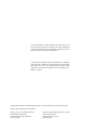
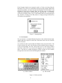
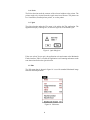
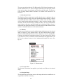
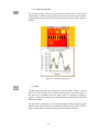
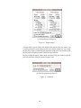
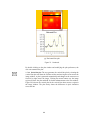
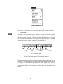
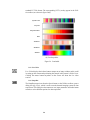
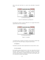
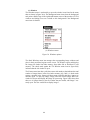
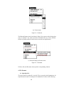
NASA Technical Memorandum 4687
TIA Software User’s Manual
K. Elliott Cramer
Langley Research Center • Hampton, Virginia
Hazari I. Syed
Analytical Services & Materials, Inc. • Hampton, Virginia
National Aeronautics and Space Administration
Langley Research Center • Hampton, Virginia 23681-0001
September 1995
The use of trademarks or names of manufacturers in this report is for
accurate reporting and does not constitute an official endorsement,
either expressed or implied, of such products or manufacturers by the
National Aeronautics and Space Administration.
Arvind R. Prabhu, Analytical Services & Materials, Inc., Hampton,
Virginia, has also contributed to the development of the Thermal Imaging Application. Work was supported under contracts NAS119236 and NAS1-20043 with Analytical Services & Materials, Inc.,
Hampton, Virginia.
Available electronically at the following URL address: http://techreports.larc.nasa.gov/ltrs/ltrs.html
Printed copies available from the following:
NASA Center for AeroSpace Information
800 Elkridge Landing Road
Linthicum Heights, MD 21090-2934
(301) 621-0390
National Technical Information Service (NTIS)
5285 Port Royal Road
Springfield, VA 22161-2171
(703) 487-4650
Contents
1.0. Introduction . . . . . . . . . . . . . . . . . . . . . . . . . . . . . . . . . . . . . . . . . . . . . . . . . . . . . . . . . . . . . . . . . . . . 1
2.0. Installation and Start-Up . . . . . . . . . . . . . . . . . . . . . . . . . . . . . . . . . . . . . . . . . . . . . . . . . . . . . . . . . . 1
2.1. Hardware Installation . . . . . . . . . . . . . . . . . . . . . . . . . . . . . . . . . . . . . . . . . . . . . . . . . . . . . . . . . . . 1
2.2. Software Installation . . . . . . . . . . . . . . . . . . . . . . . . . . . . . . . . . . . . . . . . . . . . . . . . . . . . . . . . . . . 2
3.0. Operation . . . . . . . . . . . . . . . . . . . . . . . . . . . . . . . . . . . . . . . . . . . . . . . . . . . . . . . . . . . . . . . . . . . . . . 2
3.1. Running TIA . . . . . . . . . . . . . . . . . . . . . . . . . . . . . . . . . . . . . . . . . . . . . . . . . . . . . . . . . . . . . . . . . 2
3.2. User Interface . . . . . . . . . . . . . . . . . . . . . . . . . . . . . . . . . . . . . . . . . . . . . . . . . . . . . . . . . . . . . . . . . 3
3.3. Apple Menu . . . . . . . . . . . . . . . . . . . . . . . . . . . . . . . . . . . . . . . . . . . . . . . . . . . . . . . . . . . . . . . . . . 4
3.4. File Menu . . . . . . . . . . . . . . . . . . . . . . . . . . . . . . . . . . . . . . . . . . . . . . . . . . . . . . . . . . . . . . . . . . . . 4
3.4.1. New . . . . . . . . . . . . . . . . . . . . . . . . . . . . . . . . . . . . . . . . . . . . . . . . . . . . . . . . . . . . . . . . . . . . . 5
3.4.2. Open . . . . . . . . . . . . . . . . . . . . . . . . . . . . . . . . . . . . . . . . . . . . . . . . . . . . . . . . . . . . . . . . . . . . . 5
3.4.3. Close . . . . . . . . . . . . . . . . . . . . . . . . . . . . . . . . . . . . . . . . . . . . . . . . . . . . . . . . . . . . . . . . . . . . 8
3.4.4. Save PICT . . . . . . . . . . . . . . . . . . . . . . . . . . . . . . . . . . . . . . . . . . . . . . . . . . . . . . . . . . . . . . . . 8
3.4.5. Save Selection As and Save Plot Values As . . . . . . . . . . . . . . . . . . . . . . . . . . . . . . . . . . . . . . 8
3.4.6. Print . . . . . . . . . . . . . . . . . . . . . . . . . . . . . . . . . . . . . . . . . . . . . . . . . . . . . . . . . . . . . . . . . . . . . 9
3.4.7. Quit . . . . . . . . . . . . . . . . . . . . . . . . . . . . . . . . . . . . . . . . . . . . . . . . . . . . . . . . . . . . . . . . . . . . . 9
3.5. Edit . . . . . . . . . . . . . . . . . . . . . . . . . . . . . . . . . . . . . . . . . . . . . . . . . . . . . . . . . . . . . . . . . . . . . . . . . 9
3.5.1. Undo. . . . . . . . . . . . . . . . . . . . . . . . . . . . . . . . . . . . . . . . . . . . . . . . . . . . . . . . . . . . . . . . . . . . 10
3.5.2. Cut . . . . . . . . . . . . . . . . . . . . . . . . . . . . . . . . . . . . . . . . . . . . . . . . . . . . . . . . . . . . . . . . . . . . . 10
3.5.3. Copy Selection . . . . . . . . . . . . . . . . . . . . . . . . . . . . . . . . . . . . . . . . . . . . . . . . . . . . . . . . . . . . 10
3.5.4. Paste . . . . . . . . . . . . . . . . . . . . . . . . . . . . . . . . . . . . . . . . . . . . . . . . . . . . . . . . . . . . . . . . . . . . 10
3.5.5. Clear . . . . . . . . . . . . . . . . . . . . . . . . . . . . . . . . . . . . . . . . . . . . . . . . . . . . . . . . . . . . . . . . . . . . 10
3.5.6. Select All . . . . . . . . . . . . . . . . . . . . . . . . . . . . . . . . . . . . . . . . . . . . . . . . . . . . . . . . . . . . . . . . 10
3.5.7. Flip Horizontal and Flip Vertical . . . . . . . . . . . . . . . . . . . . . . . . . . . . . . . . . . . . . . . . . . . . . . 10
3.5.8. Deallocate Frame . . . . . . . . . . . . . . . . . . . . . . . . . . . . . . . . . . . . . . . . . . . . . . . . . . . . . . . . . . 11
3.6. Enhance . . . . . . . . . . . . . . . . . . . . . . . . . . . . . . . . . . . . . . . . . . . . . . . . . . . . . . . . . . . . . . . . . . . . 11
3.6.1. Previous Filter . . . . . . . . . . . . . . . . . . . . . . . . . . . . . . . . . . . . . . . . . . . . . . . . . . . . . . . . . . . . 11
3.6.2. Original Image . . . . . . . . . . . . . . . . . . . . . . . . . . . . . . . . . . . . . . . . . . . . . . . . . . . . . . . . . . . . 11
3.6.3. Smooth . . . . . . . . . . . . . . . . . . . . . . . . . . . . . . . . . . . . . . . . . . . . . . . . . . . . . . . . . . . . . . . . . . 12
3.6.4. Sharpen . . . . . . . . . . . . . . . . . . . . . . . . . . . . . . . . . . . . . . . . . . . . . . . . . . . . . . . . . . . . . . . . . 12
3.6.5. Reduce Noise . . . . . . . . . . . . . . . . . . . . . . . . . . . . . . . . . . . . . . . . . . . . . . . . . . . . . . . . . . . . . 12
3.6.6. Add Noise . . . . . . . . . . . . . . . . . . . . . . . . . . . . . . . . . . . . . . . . . . . . . . . . . . . . . . . . . . . . . . . 12
3.6.7. Convolve . . . . . . . . . . . . . . . . . . . . . . . . . . . . . . . . . . . . . . . . . . . . . . . . . . . . . . . . . . . . . . . . 13
3.6.8. Modulus . . . . . . . . . . . . . . . . . . . . . . . . . . . . . . . . . . . . . . . . . . . . . . . . . . . . . . . . . . . . . . . . . 14
3.6.9. Enhance Contrast . . . . . . . . . . . . . . . . . . . . . . . . . . . . . . . . . . . . . . . . . . . . . . . . . . . . . . . . . . 14
3.6.10. Apply LUT. . . . . . . . . . . . . . . . . . . . . . . . . . . . . . . . . . . . . . . . . . . . . . . . . . . . . . . . . . . . . . 14
3.7. Analysis . . . . . . . . . . . . . . . . . . . . . . . . . . . . . . . . . . . . . . . . . . . . . . . . . . . . . . . . . . . . . . . . . . . . 15
3.7.1. Show Histogram. . . . . . . . . . . . . . . . . . . . . . . . . . . . . . . . . . . . . . . . . . . . . . . . . . . . . . . . . . . 15
3.7.2. Statistics . . . . . . . . . . . . . . . . . . . . . . . . . . . . . . . . . . . . . . . . . . . . . . . . . . . . . . . . . . . . . . . . . 16
3.7.3. Column Average Plot. . . . . . . . . . . . . . . . . . . . . . . . . . . . . . . . . . . . . . . . . . . . . . . . . . . . . . . 17
3.7.4. Plot . . . . . . . . . . . . . . . . . . . . . . . . . . . . . . . . . . . . . . . . . . . . . . . . . . . . . . . . . . . . . . . . . . . . . 17
3.7.4.1. Average region plot . . . . . . . . . . . . . . . . . . . . . . . . . . . . . . . . . . . . . . . . . . . . . . . . . . . . . 19
3.7.4.2. Linear plot . . . . . . . . . . . . . . . . . . . . . . . . . . . . . . . . . . . . . . . . . . . . . . . . . . . . . . . . . . . . 20
3.7.4.3. Horizontal-line plot . . . . . . . . . . . . . . . . . . . . . . . . . . . . . . . . . . . . . . . . . . . . . . . . . . . . . 21
3.7.4.4. Vertical-line plot . . . . . . . . . . . . . . . . . . . . . . . . . . . . . . . . . . . . . . . . . . . . . . . . . . . . . . . 22
iii
3.8. Special . . . . . . . . . . . . . . . . . . . . . . . . . . . . . . . . . . . . . . . . . . . . . . . . . . . . . . . . . . . . . . . . . . . . . 23
3.8.1. Animate . . . . . . . . . . . . . . . . . . . . . . . . . . . . . . . . . . . . . . . . . . . . . . . . . . . . . . . . . . . . . . . . . 24
3.8.2. LUT’s . . . . . . . . . . . . . . . . . . . . . . . . . . . . . . . . . . . . . . . . . . . . . . . . . . . . . . . . . . . . . . . . . . . 25
3.8.3. Live Video . . . . . . . . . . . . . . . . . . . . . . . . . . . . . . . . . . . . . . . . . . . . . . . . . . . . . . . . . . . . . . . 26
3.8.4. SnapShot . . . . . . . . . . . . . . . . . . . . . . . . . . . . . . . . . . . . . . . . . . . . . . . . . . . . . . . . . . . . . . . . 26
3.8.5. Demo . . . . . . . . . . . . . . . . . . . . . . . . . . . . . . . . . . . . . . . . . . . . . . . . . . . . . . . . . . . . . . . . . . . 29
3.8.6. Time Derivative . . . . . . . . . . . . . . . . . . . . . . . . . . . . . . . . . . . . . . . . . . . . . . . . . . . . . . . . . . . 29
3.8.7. Normalize. . . . . . . . . . . . . . . . . . . . . . . . . . . . . . . . . . . . . . . . . . . . . . . . . . . . . . . . . . . . . . . . 31
3.8.8. Diffusivity . . . . . . . . . . . . . . . . . . . . . . . . . . . . . . . . . . . . . . . . . . . . . . . . . . . . . . . . . . . . . . . 32
3.8.9. Save SnapShot . . . . . . . . . . . . . . . . . . . . . . . . . . . . . . . . . . . . . . . . . . . . . . . . . . . . . . . . . . . . 32
3.9. Windows. . . . . . . . . . . . . . . . . . . . . . . . . . . . . . . . . . . . . . . . . . . . . . . . . . . . . . . . . . . . . . . . . . . . 33
4. File Formats . . . . . . . . . . . . . . . . . . . . . . . . . . . . . . . . . . . . . . . . . . . . . . . . . . . . . . . . . . . . . . . . . . . . 34
4.1. Input Data File . . . . . . . . . . . . . . . . . . . . . . . . . . . . . . . . . . . . . . . . . . . . . . . . . . . . . . . . . . . . . . . 34
4.2. Output Data File . . . . . . . . . . . . . . . . . . . . . . . . . . . . . . . . . . . . . . . . . . . . . . . . . . . . . . . . . . . . . . 36
5. Glossary . . . . . . . . . . . . . . . . . . . . . . . . . . . . . . . . . . . . . . . . . . . . . . . . . . . . . . . . . . . . . . . . . . . . . . . 37
6. Troubleshooting . . . . . . . . . . . . . . . . . . . . . . . . . . . . . . . . . . . . . . . . . . . . . . . . . . . . . . . . . . . . . . . . . 38
Bibliography . . . . . . . . . . . . . . . . . . . . . . . . . . . . . . . . . . . . . . . . . . . . . . . . . . . . . . . . . . . . . . . . . . . . . . 39
iv
1.0. Introduction
This user’s manual describes the installation and operation of TIA, the ThermalImaging acquisition and processing Application, developed by the Nondestructive
Evaluation Sciences Branch at NASA Langley Research Center, Hampton,
Virginia.
TIA is a user friendly graphical interface application for the Macintosh II and
higher series computers. The software has been developed to interface with the
Perceptics/Westinghouse PixelPipe and PixelStore NuBus cards and the GW
Instruments MacADIOS input/output (I/O) card for the Macintosh for imaging
thermal data. The software is also capable of performing generic imageprocessing functions. For a quick start in acquiring images using TIA, turn to section 3.8.4.
2.0. Installation and Start-Up
2.1. Hardware Installation
The portable thermal-imaging system hardware is a user installable product. The
hardware requirements are a Macintosh II family personal computer, PixelPipe
and PixelStore image processing cards, a MacADIOS A/D I/O card and heat
lamps with a trigger box. The NuBus interface cards should be installed inside the
Macintosh as shown in figure 1.
Macintosh monitor
Camera controller
and monitor
Power supply
Macintosh video card
PixelPipeTM card
PixelStoreTM card
Infrared camera
MacAdiosTM card
ABO box
Trigger box
Figure 1. System hardware setup.
Quartz/flash
lamps
The MacADIOS I/O card is connected by a ribbon cable to an analog break-out
(ABO) box, which is connected to a trigger box by a BNC video cable. The trigger box is used to power the quartz tube or flash tube lamps. The RS-170 video
output from the infrared (IR) camera is fed to the video-in connector of the
PixelPipe image-processor card by a BNC video cable. This connection should
be made with the video IN1 line of the PixelPipe cards. TIA controls the synchronization of the heat input and data acquisition.
2.2. Software Installation
Figure 2 illustrates the icons for the software found on the accompanying disk,
including the application program, TIA V2.0 and the TurboDrivers file. TIA is
the executable program for the thermal-imaging system. TurboDrivers contains
the device driver for the MacADIOS I/O interface card that is manufactured by
GW Instruments. These drivers are used to control the heat lamps during data
acquisition. The acqdatafile is an ASCII text input data file that contains the initial setup parameters for the thermal-imaging setup. The icons labeled xyz.pic and
xyz.nv are the icons for output data written from TIA. The first is for an image
saved as a picture file, and the second is the NuVision data saved for the time
series of images that are collected.
To install the software, simply select all the icons on the disk and drag them from
the floppy disk to a new folder on the destination hard drive. Holding down the
shift key allows multiple selection of icons. TIA, TurboDrivers, and acqdatafile
must coexist in the same folder.
TIA V2.0
TurboDrivers
xyz.pic
acqdatafile
xyz.nv
Figure 2. Software icons.
3.0. Operation
3.1. Running TIA
The TIA application is a Macintosh program for use with the PixelStore and
PixelPipe image-processing cards. To run TIA from the standard Finder desktop or MultiFinder desk accessory, simply double click on the application icon. If
the Perceptics boards are properly installed in the Macintosh, the application will
run in the interactive acquisition mode.
2
If the Perceptics boards are not properly seated, or if they are missing from the
Macintosh, TIA will run as a stand-alone image-processing program without data
acquisition capability. All menu items that are dependent on the PixelPipe and
PixelStore cards will be dimmed. When TIA is being used as a stand-alone
image-processing program, a warning message is displayed (fig. 3). This message
will let the user know which, if any, of the installed cards are not functioning as
they should be. Clicking on the Okay button or simply pressing the Return key
will continue the application.
Figure 3. Warning dialog.
3.2. User Interface
The user interface is a standard Macintosh interface with available functions highlighted under their respective menu items. Each menu item in the user interface
will be discussed.
Two useful tools can be opened under the Windows menu: Info and Utilities. The
Utilities window (fig. 4(a)) is the collection of tools available for basic image processing and acquisition. The color look-up table (LUT) in the Utilities window
shows the current LUT in use and can be changed to any six predefined color
tables. Tools that are available through the Utilities window are also available
through menu items and are described throughout this manual.
(a) Utilities window.
Figure 4. Utilities and Info.
3
(b) Info window.
The Info window (fig. 4(b)) contains updated cursor information on the active
image window. Listed in the Info window are the minimum and maximum pixel
values of the current image frame and also the global minimum and maximum
values of the entire image data set. Mean and standard deviation results are also
printed for the region of interest (ROI) that is evaluated.
3.3. Apple Menu
The Apple menu contains only one TIA-specific item, About TIA. When About
TIA is selected, a dialog box is displayed (fig. 5), which gives the version and
credits to the developers of TIA. Clicking the mouse button once makes the dialog
box disappear. The suggested memory allocation is 4000 kB = 4 MB. To increase
the suggested memory allocation, refer to the Macintosh User’s Manual for setting application memory size. For large image files, a larger memory allocation
may be necessary. Of the 4 megabytes (MB) set aside for the application, 3.3 MB
are available for loading the image data. The remaining 700 kB is used to run the
application.
Figure 5. About TIA.
The remaining items in the Apple menu are system specific (e.g., desk accessories
and the active applications in MultiFinder).
3.4. File Menu
The file menu is used for all file input-output and printing. Since TIA is not a traditional document-processing application, its File menu, as shown in figure 6, differs from the standard New-Open-Close format. The File menu is used for loading
images from Macintosh disks or PixelStore smart memory into the TIA application memory and for loading and saving a variety of other data files and look-up
tables. The File menu is also used to print images and various plots generated by
the application. The individual menu items are described.
4
Figure 6. File menu.
3.4.1. New
The New menu has not been implemented in the current software version.
3.4.2. Open
The Open menu item enables the user to load an image data set or an existing
color look-up table. The Open pull-down menu items are Open Image, Import
Image, Card Memory and Load LUT.
The Open Image selection from the File menu or the Open tool from the Utilities
toolbox opens an existing experimental data set created from a disk by the applications TIA and Custom NuVision. Selecting an image data set from the disk displays an image, as shown in figure 7(a), with the appropriate parameters filled in
as they are defined in the data file. The image data set has a set of 32 frames with
each image having a 256 × 256 pixel size. A region of interest can be selected as
shown by the dashed-box region in the image. The selected region shown has a
width of 203 pixels and a height of 182 pixels. The user can either open all
32 frames in the data set by clicking the radio button All or select a starting frame
and an ending frame by selecting the radio button From. The entire image can be
selected by clicking the button Select Entire Image and can be deselected by
clicking the Undo Selection button. Clicking the Okay button (fig. 7(a)) will open
the images from the disk. The file-open operation can be aborted by clicking the
Cancel button.
(a) Selection from Open Image menu item, including ROI.
Figure 7. Options under Open pull-down menu.
5
Import Image opens an image data set stored in binary format on the disk. The
image data set can be 1 byte, 2 bytes, or 4 bytes in depth. Selecting Import Image
opens a window, as shown in figure 7(b).
(b) Import Image window.
Figure 7. Continued.
The parameters that describe the data set should be selected appropriately so that
TIA can open the images correctly. Incorrect parameters will result in the images
being skewed or noisy. The check selection for Previous Region of Interest indicates whether or not there is an existing ROI that is defined. Leaving the previous
ROI unchecked causes the window (fig. 7(a)) to open when the imported file is
opened. If the previous ROI is checked, the images are opened within the bounds
of the ROI.
Only one radio button can be selected for the image data type: 8-bit, 16-bit
Signed, 16-bit Unsigned, or 32-bit Floating Point. Two-byte data (16 bits) can be
swapped by checking the Swap Bytes selection. Checking is necessary if there is a
need to import data from an IBM PC compatible or a DEC workstation computer.
The dimensions of the image data set need to be correctly specified in the boxes
labeled Width and Height. If there is any header offset (in bytes) before the start of
the image data, this condition needs to be entered in the Offset box. The total
number of image frames in the data set is entered in the Frames box. Clicking
Open opens the images, as shown in figure 7(c), while Cancel aborts the Import
Image function.
6
(c) Open tile window.
Figure 7. Continued.
The Card Memory selection from the File menu or the Open Card tool from the
Utilities toolbox opens the set of acquired images from the PixelStore onboard
memory and displays the images shown in figure 7(c). Selecting this function
opens the same window as the Open Image function does, as shown in figure 7(a).
(d) Open tile.
Figure 7. Concluded.
Clicking Open opens the images (fig. 7(c)). Once the image tiles are open, clicking on any image tile will open that image for processing and analysis. Figure 7(d)
shows tile Frame 12 being opened from the several image tiles in data set
7
Q-CYCLE-8-16B. Any number of tiles can be opened and displayed
simultaneously.
3.4.3. Close
The Close function under the File menu closes any window that is open. A window also can be closed by clicking on the top left corner box of the window.
3.4.4. Save PICT
The Save PICT selection from the File menu saves the image frame or an image
region to the disk in the Macintosh standard PICT format. This saved-image file
can be opened from any graphics application that has the option to open PICT
files.
3.4.5. Save Selection As and Save Plot Values As
The Save Selection As and Save Plot Values As menu items let the user save an
image or the plot values to the disk. If the window that is being saved is an image,
the save selection puts up a custom Save Image box, as shown in figure 8. The
user can save the image data as a raw NuVision Data set that TIA and Custom
NuVision applications can open by selecting the radio button NuVision Data. If a
PICT file is needed, switching the radio button to PICT will save the data in this
format. The Save Plot Values As menu comes up when a Plot window is the current window selected. See section 3.7.4 for more information on Plot.
Figure 8. Save Image.
If the window being saved has a Plot, the Save Plot Values selection opens a standard Save dialog box for saving the individual x, y data values from the graph.
The stored data are in standard plot-text format that can be used to open with other
plotting applications.
8
3.4.6. Print
The Print selection sends the contents of the selected window to the printer. The
printer needs to be selected from the Apple menu item Chooser. The printer can
be a LaserWriter, PostScript laser printer, or a color printer.
3.4.7. Quit
The Quit selection under the File menu is for exiting the TIA application. The
application displays a dialog box, as shown in figure 9, to confirm the Quit.
Figure 9. Quit dialog box.
If the user selects Yes (to quit), the application exits and returns to the Macintosh
Finder interface. If No is selected, the application is still running and returns to the
state that existed before the Quit selection.
3.5. Edit
The Edit menu that is shown in figure 10 is used for standard Macintosh image
transfers and manipulations.
Figure 10. Edit menu.
9
3.5.1. Undo
The Undo item under the Edit menu cancels the last-performed operation on the
image.
3.5.2. Cut
The Cut menu has not been implemented in the current software version.
3.5.3. Copy Selection
The Copy Selection menu enables the user to copy an image or an image region
onto the Macintosh clipboard. This image then can be pasted to any graphics
design application for publication and archival of results.
Note: Save Image As from the File menu selection that is discussed in figure 8
performs the same function if the graphics application can open a PICT file. For
larger images, this is usually the better option.
3.5.4. Paste
The Paste menu has not been implemented in the current software version.
3.5.5. Clear
The Clear menu has not been implemented in the current software version.
3.5.6. Select All
The user can select the Select All menu item to select the entire image region for
either copying or for performing image analysis using the imaging tools from the
Utilities toolbox.
3.5.7. Flip Horizontal and Flip Vertical
The Flip Horizontal and the Flip Vertical menu items can be selected from the
Edit menu or from the Utilities toolbox. The user can flip either the entire image
or a ROI. If a flip ROI is desired, the user must select the ROI before the Flip
Horizontal or Flip Vertical menu item is selected. A dialog box, as shown in
figure 11, opens for the user’s input.
Figure 11. Flip Image dialog box.
10
The user can perform either the Flip Horizontal or Flip Vertical operation on the
current frame ROI or on a series of image frames ROI. The flip on the current
frame can be undone by performing an Undo from the Edit menu. The flip on a
series of image frames cannot be undone. Use caution if the data need to be
preserved.
3.5.8. Deallocate Frame
The Deallocate Frame menu item is useful when the user is opening a data set
with a large number of images. Since the minimum application memory is limited
to available Macintosh resident memory, there are times when not all the images
will be loaded into the application memory. If there is memory enough to open
40 frames, and the file has images totaling 64 frames, the user can deallocate
some frames so that more unopened images can be displayed. When a frame is
deallocated from application memory, the Frames item under the Windows menu
will have a diamond check next to the deallocated frame.
3.6. Enhance
Enhance menu functions are used to perform image enhancements on the selected
image or images by using different filters. The filter functions that are implemented are Smooth, Sharpen, Reduce Noise, Add Noise, Convolve, and Modulus.
Filtering is not limited to rectangular selections. The entire image will be filtered
if no selection is active. Automatic contrast enhancement and application of the
LUT to the enhanced image are also implemented through this menu. (See
fig. 12.)
Figure 12. Enhance menu.
3.6.1. Previous Filter
The Previous Filter menu item applies a previously used filter to the selected
image.
3.6.2. Original Image
The Original Image menu item retrieves the image that has been modified to its
original state from disk or memory.
11
3.6.3. Smooth
The Smooth filter blurs (softens) the selected area or the entire image and can be
used to reduce noise in an image. By default, a 3 × 3 kernel is used for smoothing,
but it can be changed to any kernel size, as shown in the dialog box (fig. 13).
Figure 13. Filter dialog box.
3.6.4. Sharpen
The Sharpen filter increases the contrast and accentuates detail in the selection but
may also accentuate noise. To minimize noise, the user can Smooth or Reduce
Noise before using Sharpen. By default, a 3 × 3 pixel-size kernel is used for
smoothing but can be changed to any kernel size, as shown in the dialog box
(fig. 13).
3.6.5. Reduce Noise
Reduce Noise is a “median filter,” in which each pixel is replaced with the median
value of its nine nearest neighbors. Reducing noise is a time-consuming operation
because for each pixel in the selection, the nine pixels in the 3 × 3 neighborhood
must be sorted, and the center pixel must be replaced with the median value (the
fifth). By default, a 3 × 3 kernel is used for smoothing, but the kernel can be
changed to any size, as shown in the dialog box (fig. 13).
3.6.6. Add Noise
Add Noise is a feature that is implemented specifically for comparing finite element results to experimental results. By default, a value of 10 is chosen for the
multiplier to the Gaussian derivative, but the value can be changed, as shown in
figure 14.
Figure 14. Add Noise dialog box.
12
The Gaussian distribution routine is used to provide a normal distribution with a
standard deviation of 1. The image data are changed by adding the deviate error to
these data as shown in the expression below.
Image new = Image old + GaussNoise × [ Error ]
Noise can be added to a single image or a series of images in time.
3.6.7. Convolve
The Convolve function does spatial convolutions using kernels that are read from
a text file that can be up to 63 × 63 pixels in size. Use the Macintosh TeachText
systems application to create a new convolution kernel or to examine an existing
kernel.
(a) Convolution dialog box.
Figure 15. Convolve function.
When the convolution function is selected from the Enhance menu or the Utilities
tool, a dialog box (fig. 15(a)) opens. The convolution can be done on a single
image or a sequence of images. Pressing the Okay button opens a dialog box that
locates and selects the convolution kernel file. An example of a 7 × 7 Winfree
convolution filter is shown below (fig. 15(b)).
10
5
2
1
2
5
10
5
0
-3
-4
-3
0
5
2
-3
-6
-7
-6
-3
2
1
-4
-7
-8
-7
-4
1
2
-3
-6
-7
-6
-3
2
5
0
-3
-4
-3
0
5
10
5
2
1
2
5
10
(b) Winfree convolution filter (7 × 7).
Figure 15. Concluded.
13
3.6.8. Modulus
The Modulus (Mod) function menu can be a useful image-processing tool. The
Mod Value entered in the dialog box is used to do a recursive mod with the image
pixel until no further mod function can be done; that is, Pixel value = (Pixel value)
Mod (Mod Value) is repeated until no more mod functions can be done. The mod
function can be performed for a single image or a sequence of images. Figure 16
shows the Modulus dialog box.
Figure 16. Modulus dialog box.
3.6.9. Enhance Contrast
The Enhance Contrast menu item from the Enhance menu or the Utilities toolbox
enhances the image region of interest by recalculating the minimum and maximum values in the ROI and by scaling the pixel values to the 256-level LUT. This
action changes the LUT gray map on the Utilities toolbox. Figure 17 shows the
images before and after applying Enhance Contrast to the image ROI.
Before.
After.
Figure 17. Before and after Enhance Contrast applied to image ROI.
3.6.10. Apply LUT
Apply LUT can be selected from the Enhance menu or the Utilities toolbox. This
menu function should be used with caution because it destroys the original image
and modifies the screen pixel values to reflect the enhanced image. Figure 18
14
shows the image region for which the LUT has been applied to the enhanced
region.
Figure 18. Apply LUT to Enhanced region.
The region that has been enhanced will be modified by using the new minimum
and maximum values with the region and by scaling to the 0–255 limits of the
color LUT.
3.7. Analysis
The Analysis menu includes Show Histogram, Statistics, Column Average Plot,
and Plot items (fig. 19). Each menu item is explained in detail in the following
sections.
Figure 19. Analysis menu.
3.7.1. Show Histogram
The Show Histogram menu item can be selected from the Analysis menu or the
Utilities toolbox. An image ROI must be selected before the histogram can be
generated. The histogram plot, which shows the pixel distribution in the ROI (in
an image), can be modified for printing by customizing the plot parameters. Customizing is explained in more detail in section 3.7.4 on Plot. A window showing
the histogram of the pixel distribution is drawn for the image ROI (fig. 20).
15
Figure 20. Histogram plot.
The histogram plot can be printed to hard copy by selecting the Print Plot menu
item from the File menu.
3.7.2. Statistics
The Statistics selection from the Analysis menu or the Utilities toolbox gives the
image ROI statistics shown in the Info box (fig. 21). The minimum and maximum
values in the ROI, including the number of pixel values, the average pixel value,
and the standard deviation are printed in the Info window.
Figure 21. Region statistics.
16
3.7.3. Column Average Plot
The Column Average Plot menu item from the Analysis menu or the Utilities
toolbox draws a column average plot from a previously selected region of interest.
A plot is shown (fig. 22) that represents the average pixel values of the columns in
the ROI.
Figure 22. Column average plot.
3.7.4. Plot
The Plot menu item under the Analysis menu or the Utilities toolbox is used to
make an X-Y plot. The plot may be a horizontal-line plot, a vertical-line plot, or a
line plot in any orientation across the image. Also, if a sequence of images is
opened, a region on an image can be selected, and an average time profile of the
ROI can be plotted.
The plot can be customized for viewing and printing. Double clicking anywhere
inside the plot window opens a plot preferences dialog box (fig. 23(a)). This dialog box enables the user to change settings for the entire plot window.
17
(a) Plot preferences dialog box.
Figure 23. Graph settings.
The user input boxes are filled with default values based on the plot values. Any
or all the parameters can be changed for the plot, and the changes are set by clicking the Okay button. Customizing the appearance of the plot is useful when sending the plot to a PostScript printer for a hard-copy reference.
Double clicking the mouse button on the title area of the plot window opens the
plot title preference dialog box shown in figure 23(b).
(b) Plot title preference dialog box.
Figure 23. Continued.
18
Double clicking the mouse button on the X-axis region of the plot window opens
the plot X-Axis Settings dialog box shown in figure 23(c).
(c) Plot X-Axis Settings dialog box.
Figure 23. Continued.
Double clicking the mouse button on the Y-axis region of the plot window opens
the plot X-Axis Settings dialog box shown in figure 23(d).
(d) Plot Y-Axis Settings dialog box.
Figure 23. Continued.
The dialog boxes in figure 23 enable customization of the selected individual
parameters on the plot.
3.7.4.1. Average region plot. The average region plot generates the average
temperature-time profile of the image sequence data. An image region across the
image window should be selected first. If the user then selects the Plot menu item
or the Plot tool in the Utilities toolbox, the plot can be generated as shown in
figure 23(e).
19
(e) Average plot.
Figure 23. Continued.
The user can customize the plot by double clicking on the plot window and modifying the plot preferences.
3.7.4.2. Linear plot. The linear plot generates a plot from data that is derived by
drawing a line in any orientation across an image window. By selecting the linear
plot tool from the Utilities toolbox, the user can draw a line across the image window; then, by selecting the Plot menu item or the Plot tool in the Utilities toolbox,
the user can generate the plot shown in figure 23(f).
20
(f) Linear plot.
Figure 23. Continued.
The user can customize the plot by double clicking on the plot window and modifying the plot preferences.
3.7.4.3. Horizontal-line plot. The user generates the horizontal-line plot by selecting the horizontal-line-plot tool from the Utilities toolbox and moving the cursor
across the image window. A plot is generated automatically and changes as the
cursor moves from top to bottom across the image. Clicking the mouse button
over the image region will draw the plot and hold it for further enhancements to
the Plot window. Figure 23(g) shows the horizontal plot for the horizontal line
drawn across a region in the image window. The plot clearly shows the differences in pixel intensities across the line.
21
(g) Horizontal-line plot.
Figure 23. Continued.
By double clicking on the plot window and modifying the plot preferences, the
user can customize the plot.
3.7.4.4. Vertical-line plot. The user generates the vertical-line plot by selecting the
vertical-line-plot tool from the Utilities toolbox and moving the cursor across the
image window. A plot is generated automatically and changes as the cursor moves
from left to right across the image. Clicking the mouse button over the image
region will draw the plot and hold for further enhancements to the Plot window.
Figure 23(h) shows the vertical plot for the vertical line drawn across a region in
the image window. The plot clearly shows the differences in pixel intensities
across the line.
22
(h) Vertical-line plot.
Figure 23. Concluded.
The user can customize the plot by double clicking on the plot window and modifying the plot preferences.
3.8. Special
The Special menu items shown in figure 24 enable the user to perform image
acquisition and data processing on the acquired images. These image-processing
functions interact with the installed Perceptics cards. The PixelPipe card is a
frame grabber with an onboard digital signal processor (DSP) and an arithmetic
logic unit (ALU), and the SmartStore card stores the sequential real-time images
in memory. The SmartStore card has 32 MB of random access memory (RAM)
available for image storage.
23
Figure 24. Special menu.
Each of the special menu items is described in detail in the sections that follow.
3.8.1. Animate
Animate is used for playing a movie sequence of images from memory. These
images can be loaded to memory from the image-processing card memory or from
the images stored on hard disk. The images being loaded should have at least two
or more images for Animate to work. Figures 25(a) and 25(b) show the Animate
controls and Animate window with image 15 being displayed.
Total images
Speed control
Looper
Rewind
Pause
Fast Forward
Back Image
Current image #
Scroll Bar
Fwd. Image
(a) Animate controls.
Figure 25. Animate controls and window for image 15
The Animate control bar contains all the information regarding the image data set
in memory. The current data set in memory used for this example contains a set of
32 images. The various buttons for Animate are shown in figure 25(a). The user
can scale the image contained in the Animate window to fit the entire window or
to maintain the aspect ratio by holding the shift key down and clicking the mouse
button.
24
(b) Animate window.
Figure 25. Concluded.
3.8.2. LUT’s
There are seven predefined LUT’s in the application. They are the standard System Colors, Grayscale, Temperature scale, Reds, Fleshtones, Earthtones, and
Rainbow LUT’s. The LUT’s can also be reversed by selecting the Invert LUT
menu item. Figure 26(a) shows the LUT menu as it appears under the Special
menu.
(a) LUT menu.
Figure 26. LUT’s options.
New LUT’s also can be loaded for use with the images in memory from the Open
pull-down menu item Load LUT under the File menu. The LUT file has to be in a
25
standard LUT file format. The corresponding LUT’s (as they appear in the Utilities toolbox) are shown in figure 26(b).
System Colors
Grayscale
Temperature Rise
Reds
Fleshtones
Earthtones
Rainbow
(b) Look-up tables.
Figure 26. Concluded.
3.8.3. Live Video
Live Video displays the infrared camera output on an image window and is useful
in setting up the camera and positioning the sample in the camera’s field of view.
Clicking the mouse button anywhere on the screen will abort the live video
session.
3.8.4. SnapShot
The SnapShot menu item from the Special menu or the Utilities toolbox opens a
dialog box (fig. 27(a)), which is used to run the thermal-imaging system for data
acquisition. This dialog box has numerous user input parameters and radio button
controls to select different options for data acquisition.
26
(a) SnapShot dialog box.
Figure 27. Data acquisition.
Frame Avgs
A number from 4 to 256 must be entered for the number of live video frames averaged together to form an image tile.
Note: The product of average frames and the number of cycles should not exceed
256 while data are being acquired in 16-bit mode. Data overflow will occur if the
product is greater than 256.
Heating
The heating can be turned ON or OFF by checking the check box. If the box is
checked, continuous or pulse heating can be selected from the radio button. Continuous heating will leave the lamps on for the duration of the data acquisition
cycle. This option ignores the number-of-cycles parameter. Pulse heating turns
the lamps ON and OFF for a user specified duration (number of frames) during
each acquisition cycle.
Frame Size
The radio button selection for frame size lets the user select an image region of
128 × 128 pixels, 256 × 256 pixels, or 512 × 512 pixels for memory allocation
and storage. The image size should be selected depending on the camera’s spatial
resolution.
Background
The background check box specifies whether or not a background image is to be
acquired before the heat lamps are turned on. The background image can be useful
in reducing the noise and variations in emissivity. A background-image selection
will affect the number of image tiles being acquired.
Tiles ON
The user should specify the duration in the number of tiles that are selected and
how long the heat lamps are to stay ON with respect to the total frames that are
27
being acquired. The difference between the total number of tiles and the number
of tiles in which the lamps are ON determines how long the lamps will be in the
OFF state during each acquisition cycle.
# of Tiles
The # of Tiles entry is a value corresponding to the number of averaged sequential
images being acquired. This value can be up to the maximum allowable image
tiles for the system. The table below shows the maximum number of available
8-bit image tiles for a PixelPipe system with 32 MB memory board configuration. For example, one can acquire a maximum of 64 tiles for 8 heat-up-cooldown
cycles in the 256 × 256 image-size mode (64 * 8 = 512 is the maximum number
of 8-bit tiles).
Image Size
Number of 8 bit
Tiles
128x128
2048
256x256
512
512x512
128
Cycles
The number of cycles should be a number greater than 0. The upper limit for the
number of cycles depends on the total allowable 8-bit images for the image size
that is selected. The product of the total number of tiles being acquired and the
number of cycles should not exceed the total allowable number of 8-bit images.
Delay
The delay (frames) is the time delay that is desired during multiple-cycle acquisition (the delay between cycles). Figure 27(b) shows a schematic of a cyclic
acquisition.
On
On
Delay
Off
Delay
Off
Acquisition time
(b) Pulse-cyclic acquisition with delay.
Figure 27. Concluded.
Using quartz lamp heating (Frame Avgs = 16, Pulse heating, Background OFF,
256 × 256 Frame size, 16 Tiles ON, # of Tiles = 32, Delay = 0, i.e., the parameters in figure 26(a)) enables the quartz lamps to stay on for (16/30) * 16 = 8.53 sec
(number of frames averaged (16) divided by video-frame rate (30 fps) times the
duration (16 frames)). Though the time comes to 8.53 sec, the actual time the
lamps stay on will be slightly greater because of fractional time loss (one frame
time) in writing image data from one memory tile to the other during acquisition.
Another example parameter set uses flash-lamp heating (Frame Avgs = 4 for 16,
Pulse heating, Background ON, 256 × 256 Frame size, 1 Tile ON, # of Tiles = 32,
28
Delay = 180). The lamps flash after a background image is collected, and data are
collected for approximately 5 sec ((4 * 31 tiles)/30 fps acquisition time + 30 tiles/
30 fps lost time during tile switching). For a low number of averages (high data
collection rate), the time lost between image tiles becomes very significant. The
delay of 180 (180 * 1 average frame, or 180/30 fps = 6 sec) allows sufficient time
for the flash lamps to recharge before the next data collection cycle.
Data Dump
The user can store data to a file on disk by checking the data dump box. Turning
data dump off is useful for doing trial runs and when data storage is not required.
Trial-run data can be stored to the disk after the snapshot by selecting the Save
SnapShot menu item under the Special menu.
Reduction
A time-derivative reduction can be performed on the most recently acquired data
by checking the Data Reduction box. The evaluated-time-derivative image is
stored in a file with a <.td> extension and is displayed for viewing in a window.
Bits
The radio button Bits is used to specify the depth of the pixel data being stored.
Integer data can be 8 bits (1 byte) or 16 bits (2 bytes). The higher the depth of the
data, the greater the precision. In most thermal measurements, 16 bits is the
desired data-storage mode. Here, the default mode of storage is 16 bit.
Filename
Users enter a filename for writing the data (to disk) that is acquired from
SnapShot. The written data has a 30-byte header that is followed by the imageframe data in image sequence and binary format. The data format is explained in
more detail in the next chapter. After all the user parameters are selected and
entered, clicking Okay will start the acquisition process; clicking Cancel will quit
the SnapShot dialog. Once the acquisition has been started, clicking the Command and period keys will abort the acquisition process.
3.8.5. Demo
Demo is a customized Special menu item that can be used to set up thermal experiment demonstrations on known samples with defects. The parameters used by
Demo during SnapShot are read from the text file acqdatafile. These parameters
can be changed using any text editor.
3.8.6. Time Derivative
The user can perform time-derivative (TD) reduction on stored images in a postprocessing mode by selecting the Time Derivative menu item from the Special
menu. The image data can reside in three modes: the SmartStore card memory, a
TIA-Custom NuVision data file that is stored on disk, or a generic binary image
data set. (See fig. 28(a).)
29
(a) Time Derivative pull-down menu.
Figure 28. Time Derivative options.
The user can perform time-derivative data reduction on data that is residing in the
PixelStore memory cards by selecting the Card Memory menu item under the
Special menus Time Derivative pull-down menu or from the Utilities toolbox
tool. The Card Memory menu item can be selected only if there is image data that
has been collected using the SnapShot menu item in the Special menu.
Time derivative data reduction on TIA-Custom NuVision image data residing on
the hard disk is performed by selecting the Open File menu item under the Special
menu Time Derivative pull-down menu or from the Utilities toolbox tool.
Time derivative data reduction on generic binary image data sets residing in the
hard disk can also be performed by selecting the Import File menu item under the
Special Menu Time Derivative pull-down menu or from the Utilities toolbox tool.
Once the time derivative is selected for an image data set, a dialog box (shown
previously in fig. 7(a)) opens for the user to select a ROI. After a ROI has been
selected, another dialog box opens for calculating the time derivative, as shown in
figure 28(b).
(b) Time derivative (TD) weights dialog box.
Figure 28. Continued.
30
The TD Weights dialog box requires an input for the frames range and the frame
at which the time derivative is to be evaluated. The default values that are filled in
are the maximum image range (i.e., 1 to the maximum number of images in the
card memory or data file), and the TD are evaluated at the eighth frame (in time)
for a sequence of 32 frames (in time). Figure 28(c) shows the time-derivative
image that was evaluated based on input parameters from the TD Weights dialog
box.
(c) Time derivative image.
Figure 28. Concluded.
3.8.7. Normalize
Normalization is a useful feature for reducing the effects of uneven heating and
emissivity variations. With this technique, the thermal response curves are dependent only on thickness and diffusivity. By using different windowing techniques,
one may be able to observe defects occurring at specific times.
Three such normalization techniques have been implemented within TIA. The
output images are derived from the following equations.
n
∑ Img ( i)
1
Output image = ------------------------Img ( j )
n
Output image =
∑ Img ( i) – n × Img ( j)
i=1
n
∑ Img ( i)
i=1
Output image = ---------------------------n
Img ( j )
∑
j=1
31
where i and j take values from 1 to n, and n is the total number of sequential
images.
(a) Normalization dialog A.
Figure 29. Normalization Type dialog boxes.
The dialog boxes shown in figure 29 enable the user to toggle from the three
implemented routines for normalization.
(b) Normalization dialog B.
Figure 29. Concluded.
A normalized image is displayed on completion of the operation. Further image
processing can be done of the image by using the toolbox functions.
3.8.8. Diffusivity
The Diffusivity menu has not been implemented in the current software version.
3.8.9. Save SnapShot
Save SnapShot (under the Special menu) is used to save image data to the hard
disk that is resident in PixelStore card memory. This data set (in memory)
would have been captured by selecting SnapShot from the Special menu. This
menu item is handy when the user wishes to save the data set after doing trial-anderror experiments on samples using SnapShot.
32
3.9. Windows
The Windows menu is used mainly to open the window items listed in the menu
that are shown in figure 30(a). The Background menu item clears the background
and paints a NASA logo in the right-hand bottom corner of the monitor. All TIA
windows and dialog boxes are overlaid on this background if the Background
menu item is checked.
(a) Windows menu.
Figure 30. Windows options.
The Stack Windows menu item arranges the corresponding image windows and
plots in their predefined regions on the screen. Tile Window opens and displays
the image tiles loaded into Mac memory from either disk or PixelStore card
memory. The check mark against the Tile Window menu item in figure 30(b)
indicates that the tile window is open.
The Frames menu item has a pull-down menu with numbers that indicate the total
number of image frames in the tile window memory (fig. 30(b)). A check mark
against a number in the frames pull-down menu indicates that these images are
currently open. To open any image, simply select the desired image and a new
window will open and display the image for processing. Figure 30(b) shows that
there are 10 image frames in the tile window that are loaded, with image 5 currently open. The user would like to display image 3.
33
(b) Frames menu.
Figure 30. Continued.
The Reduced Images menu item shown in figure 30(c) opens a reduced image that
exists in memory. Any menu item that is dimmed has not yet been reduced.
Diffusivity Image cannot be used because it has not been implemented.
(c) Reduced Images pull-down menu.
Figure 30. Concluded.
Utilities, Info, and Plot menu items open the corresponding windows.
4. File Formats
4.1. Input Data File
The input data file acqdatafile is used by TIA to set up the initial parameters for
acquisition and control. An example of a standard file is shown in the following:
34
### TIA ###
0
# Background window on start-up (0-NO; 1-YES)
0
# SnapShot dialog on start-up (0-NO; 1-YES)
1
# Number of cycles
0
# Delay
32
# Number of frames
16
# Frame averages
256
# Frame size
1
# Heating (0-OFF; 1-ON)
1
# Heating Type (0-CONT; 1-PULSE)
0
# Background (0-OFF 1-ON)
16
# Number of frames for lamps ON
0
# Data dump (0-OFF; 1-ON)
16
# Data size (8 or 16)
1
# Data reduction (0-OFF; 1-ON)
testimage.nde
# File name
### TD ###
0
# Scaling (0-OFF; 1-ON)
−1
# MIN
−0.5
# MAX
### DEMO ###
1
# Number of cycles
0
# Delay
3
# Number of frames
256
# Frame averages
256
# Frame size
1
# Heating (0-OFF; 1-ON)
1
# Heating type (0-CONT; 1-PULSE)
1
# Background (0-OFF; 1-ON)
1
# Number of frames for lamps ON
0
# Data dump (0-OFF; 1-ON)
16
# Data size (8 or 16)
1
# Data reduction (0-OFF; 1-ON)
demo.nde
# File name
3
# Number of frames
0
# Scaling (0-OFF; 1-ON)
−1
# MIN
35
−0.5
# MAX
−1.0
# Weights follow
0.0
1.0
The file contents can be changed to suit the user’s sample configuration. If only
16 frames are being acquired, simply change the value 32 to 16 and modify the
time-derivative weights accordingly.
4.2. Output Data File
The output data file created by SnapShot has a 30-byte header followed by the
image data in sequence. The image data size will depend on the following: image
size, each pixel size, and the number of images that are being acquired. The
30-byte header format is shown below:
Byte 1-2
version ID
Byte 3-4
pixel size
Byte 5-6
number of rows
Byte 7-8
number of columns
Byte 9-10
number of averages on each tile
Byte 11-12
number of image tiles
Byte 13-30
unused (reserved for future use)
Byte 31
end of file image data
36
5. Glossary
ABO
An analog break-out box.
ASCII
American Standard Code for Information Interchange, a
standard for the codes assigned to text characters.
binary
Output data format.
TIA
A graphical user interface application for thermal imaging
on a Macintosh desktop computer.
acqdatafile
An ASCII input data file for the TIA application containing
initial set-up parameters.
digitizer
The hardware that converts an analog video signal into a
digital image. Also referred to as a frame grabber.
Fourier transform
A mathematical operation which transforms a time domain
signal into a frequency domain signal. In two dimensions,
Fourier transform converts a spatial image into a frequency
image. The fast-Fourier transform (FFT) algorithm is the
most popular method of computing the Fourier transform.
frame
A complete raster-scan video image.
NuBus
The expansion bus for the modular Macintosh II series and
above.
pixel
A picture element. The smallest element of an image which
is stored or displayed.
RS 170
A common monochrome video standard that has 2:1 interlace, a rate of 30 fps and a nominal resolution of 640 × 480
pixels. Most cameras have RS-170 video-signal output.
tile
An image region in memory that is mapped to the application display interface.
time derivative
Temperature image data in time is fitted to a second order
polynomial; the value of the time derivative is obtained by
taking the derivative of this polynomial at a given time.
TurboDrivers
Drivers for the MacADIOS A/D I/O interface card.
video-frame rate
Images at 30 fps.
37
6. Troubleshooting
If there are specific questions or problems regarding the TIA application usage,
please write or call
K. Elliott Cramer
Nondestructive Evaluation Sciences Branch
MS 231, NASA Langley Research Center
Hampton, VA 23681
(804) 864-4970
(804) 864-4914 (fax)
Some of the known bugs and their solutions are listed in the sections below:
A dialog box appears with a warning that the acqdatafile does not exist in the current application folder.
Locate the acqdatafile and copy it into the current application folder.
A dialog box appears with a warning that the PixelPipe and PixelStore cards
are not installed in the computer.
Make sure the cards are installed, and if not, install the cards following
the cards-installation procedure. If the cards are already installed, reseat the
cards. Restart the computer and the TIA application should recognize the
cards.
TIA warns with a dialog box that the PixelStore cards are not installed in the
computer even though they exist in the computer.
Quit the TIA application and restart TIA.
The Look-up-table scale on the utilities toolbox window goes white, and the graymap line appears noncontinuous.
Closing the utilities toolbox and reopening it will solve the problem.
Also, before starting an image acquisition using SnapShot, make sure the
utilities toolbox is closed.
NASA Langley Research Center
Hampton, VA 23681-0001
June 26, 1995
38
Bibliography
Cramer, K. E.; Syed, Hazari; and Winfree, William P.: Thermographic Detection of Cracks in Thin
Sheets. Review of Progress in Quantitative Nondestructive Evaluation—Volume 10A, Donald O.
Thompson and Dale E. Chimenti, eds., Plenum Press, 1991, pp. 1087–1094.
Syed, Hazari I.; Winfree, William P.; Cramer, K. Elliott; and Howell, Patricia A.: Thermographic
Detection of Corrosion in Aircraft Skin. Review of Progress in Quantitative Nondestructive
Evaluation—Volume 12B, Donald O. Thompson and Dale E. Chimenti, eds., Plenum Press,
1993, pp. 2035–2041.
Syed, Hazari I.; Winfree, William P.; and Cramer, K. Elliott: Processing Infrared Images of Aircraft
Lapjoints. Thermosense XIV—An International Conference on Thermal Sensing and Imaging
Diagnostic Applications, Jan K. Eklund, ed., SPIE, vol. 1682, 1992, pp. 171–177.
Winfree, William P.; and James, Patricia H.: Thermographic Detection of Disbonds. Proceedings of
the 35th International Instrumentation Symposium, ISA, 1989, pp. 183–188.
Winfree, William P.; Crews, B. Scott; Syed, Hazari; Howell, Patricia; and Cramer, K. Elliott: Thermographic Detection of Disbonds in Riveted Lap Joints. Proceedings of the 37th International
Instrumentation Symposium, ISA, 1991, pp. 1097–1105. (Available as ISA Paper 91-127.)
Winfree, William P.; Crews, B. Scott; and Howell, P. A.: Comparison of Heating Protocols for
Detection of Disbonds in Lap Joints. Review of Progress in Quantitative Nondestructive Evaluation—Volume 11A, Donald O. Thompson and Dale E. Chimenti, eds., Plenum Press, 1992,
pp. 471–478.
39
Form Approved
OMB No. 0704-0188
REPORT DOCUMENTATION PAGE
Public reporting burden for this collection of information is estimated to average 1 hour per response, including the time for reviewing instructions, searching existing data sources,
gathering and maintaining the data needed, and completing and reviewing the collection of information. Send comments regarding this burden estimate or any other aspect of this
collection of information, including suggestions for reducing this burden, to Washington Headquarters Services, Directorate for Information Operations and Reports, 1215 Jefferson
Davis Highway, Suite 1204, Arlington, VA 22202-4302, and to the Office of Management and Budget, Paperwork Reduction Project (0704-0188), Washington, DC 20503.
1. AGENCY USE ONLY (Leave blank) 2. REPORT DATE
September 1995
3. REPORT TYPE AND DATES COVERED
Technical Memorandum
4. TITLE AND SUBTITLE
5. FUNDING NUMBERS
TIA Software User’s Manual
WU 538-02-11-01
6. AUTHOR(S)
K. Elliott Cramer and Hazari I. Syed
7. PERFORMING ORGANIZATION NAME(S) AND ADDRESS(ES)
8. PERFORMING ORGANIZATION
REPORT NUMBER
NASA Langley Research Center
Hampton, VA 23681-0001
L-17471
9. SPONSORING/MONITORING AGENCY NAME(S) AND ADDRESS(ES)
10. SPONSORING/MONITORING
AGENCY REPORT NUMBER
National Aeronautics and Space Administration
Washington, DC 20546-0001
NASA TM-4687
11. SUPPLEMENTARY NOTES
Cramer: Langley Research Center, Hampton, VA; Syed: Analytical Services & Materials, Inc.,
Hampton, VA.
12a. DISTRIBUTION/AVAILABILITY STATEMENT
12b. DISTRIBUTION CODE
Unclassified–Unlimited
Subject Category 77
Availability: NASA CASI (301) 621-0390
13. ABSTRACT (Maximum 200 words)
This user’s manual describes the installation and operation of TIA, the Thermal-Imaging acquisition and processing Application, developed by the Nondestructive Evaluation Sciences Branch at NASA Langley Research Center,
Hampton, Virginia. TIA is a user friendly graphical interface application for the Macintosh II and higher series
computers. The software has been developed to interface with the Perceptics/Westinghouse PixelPipe and
PixelStore NuBus cards and the GW Instruments MacADIOS input-output (I/O) card for the Macintosh for
imaging thermal data. The software is also capable of performing generic image-processing functions.
14. SUBJECT TERMS
Infrared thermal imaging; Image processing; Nondestructive evaluation
15. NUMBER OF PAGES
42
16. PRICE CODE
A03
17. SECURITY CLASSIFICATION
OF REPORT
Unclassified
NSN 7540-01-280-5500
18. SECURITY CLASSIFICATION
OF THIS PAGE
Unclassified
19. SECURITY CLASSIFICATION
OF ABSTRACT
20. LIMITATION
OF ABSTRACT
Unclassified
Standard Form 298 (Rev. 2-89)
Prescribed by ANSI Std. Z39-18
298-102