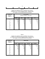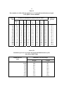
1
Sugar Research Australia Ltd. eLibrary http://elibrary.sugarresearch.com.au/ Completed projects final reports Varieties, Plant Breeding and Release 1993 Development of techniques to study root systems of sugarcane. Reghenzani, JR http://hdl.handle.net/11079/317 Downloaded from Sugar Research Australia Ltd eLibrary BUREAU OF SUGAR EXPERIMENT STATIONS QUEENSLAND, AUSTRALIA FINAL REPORT SRDC PROJECT BS56S DEVELOPMENT OF TECHNIQUES TO STUDY ROOT SYSTEMS OF SUGARCANE by J R Reghenzani SD93003 Principal investigator: Mr J R Reghenzani Research Officer Tully SES PO Box 566 TULLY Q 4854 Phone: 070 68 1488 This project was funded by the Sugar Research Council/Sugar Research and Development Corporation during the 1990-1991 financial year. BSES Publication SRDC Final Report SD93003 June, 1993 CONTENTS Page No 1. SUMMARY 1 2. BACKGROUND 1 3. PROJECT OBJECTIVES 2 4. INTRODUCTION 2 5. METHODS 3 5.1 3 3 4 4 4 5 5 6 6 5.2 5.3 6. Previous root studies 5.1.1 Root weight in soil cores 5.1.2 Root intersection studies Current root studies 5.2.1 Sample collection 5.2.2 Root washing 5.2.3 Root length and weight determination 5.2.4 Data analysis and presentation Image analysis of roots from yield decline soils RESULTS AND DISCUSSION 6.1 6.2 6.3 6.4 System modification and operation 6.1.1 Root washing 6.1.2 Root length determination Root distribution studies 6.2.1 Previous studies 6.2.1.1 Root weight in soil cores 6.2.1.2 Root intersection studies 6.2.2 Current studies 6.2.2.1 Root weight in soil cores 6.2.2.2 Root length in soil cores Sampling strategy summary Image analysis of roots from yield decline soil 6.4.1 Image analysis system 6.4.2 Spectral characteristics of yield decline roots 6.4.3 Processing of image analysis data 6.4.4 Operation of colour imaging system 6 6 6 7 8 8 8 9 9 9 10 11 12 12 12 13 14 7. DIFFICULTIES 14 8. RECOMMENDATIONS FOR FUTURE RESEARCH 14 9. PUBLICATIONS 14 10. REFERENCES 15 APPENDIX A Procedures for processing roots 32 APPENDIX B Procedures for root length measurement 35 1. SUMMARY The aim of this project, to develop quantitative, cost-effective techniques for assessing the size and extensiveness of root systems in sugarcane, has been achieved. The equipment purchased and subsequently modified, and the techniques developed, have vastly improved the capacity to study root systems of sugarcane. Modifications were made to substantially improve the operation of the hydropneumatic elutriation system imported from USA. Optimal settings of the image analysis system imported from the UK were determined for root length measurement (monochrome) and root colour (colour image processing). Macro files were written to speed the operation of the latter. The test field studied was found to have 5 km of sugarcane roots per metre of row, approximately 34 000 km per hectare. In terms of root weight, the same field had 190 g dry weight of roots per metre of row, ie 1.3 t per hectare. Root length, a new measure not possible without computer imaging technology, was found to be a better quantitative measure of root distribution. A system was developed to present data on root distribution and variability in a pictorial form using a geographic information system (GIS). The study examined root distribution to 1 metre depth. On the basis of root length, over half of the roots were in the top 300 mm. Variability in root data has caused problems for all in this field of research. There was no exception in this case. Sampling strategies were developed to allow sample size to be set within practical limits, yet meet specific statistical objectives. Labour required to extract, wash and analyse a large number of cores has been reduced using the techniques outlined in this report. Sorting of sugarcane roots from other organic material still remains a labour intensive operation which has not been overcome by this research or other work known to the author. Colour image analysis of roots from a yield decline soil is a novel and technologically advanced technique, which has potential to assist in the valuable research being conducted into the yield decline problem. The techniques developed in this project are being considered for use in a range of research projects in yield decline, plant pathology and agronomy. 2. BACKGROUND Studies of root systems in sugarcane and other crops have been restricted by time and cost of available techniques. Direct observation of root density and distribution carried out by Lawrence (1984) involved destructive sampling from pits in cane fields with consequent loss of the site for future studies. Effective techniques for the study of root systems of sugarcane are applicable to nutritional, soil physical, biological, breeding and entomological studies. An effective and extensive 2 root system is required for the absorption of nutrients and the anchorage of plants in the soil. It also influences the yield and processing quality of the sugarcane crop. Recent advances in hydropneumatic elutriation systems (HES) for separating roots from soil (Smucker et al, 1982) and computer-based image analysis systems (IAS) for measuring root length (Voorhees et al, 1980) have allowed rapid and accurate measurement of root growth. Similar equipment has been used in Australia in shallow rooted annual crops. This study evaluates its effectiveness and improves the technology of recovery of roots for the longer term sugarcane crop, which has a deeper root profile and occurs in a heterogenous range of soils in sugar industry areas. 3. PROJECT OBJECTIVES ! ! Purchase HES/IAS system. Review existing spatial root distribution data to determine a theoretical base for sampling. Establish optimum HES settings for a range of measured soil physical attributes using cores from sugarcane fields. Calibrate and determine ability of IAS system to differentiate between roots affected by important root pathogens. ! ! All of these objectives were achieved, as documented in this report. 4. INTRODUCTION Commercially available hydropneumatic elutriation systems (HES) and computer-based image analysis systems (IAS) were reviewed, and systems suitable for the task were purchased and imported. A review of previous root distribution studies was conducted to gain an insight into a theoretical base for future sampling. The review involved inspection of root distribution data and calculation of sample sizes required to meet specific statistical parameters. Figure 1 is a schematic representation of the HES manufactured by Gillisons Variety Fabrication Inc, Benzonia, USA. The system separates roots from soil by the joint action of water circulating in the washing chamber (A) and the buoyancy provided by water and air in the elutriation chamber (B). The root samples are collected in the low energy sieve (D). The HES was evaluated using cores from sugarcane fields. Substantial modifications were made to the transfer tube (C). Optimal settings for air and water pressure and washing time were determined. These developments, together with appropriate sample preparation, optimised HES operation for the range of soil physical conditions likely to be encountered. The Skye Instruments Limited IAS consists of a light box, a colour video camera, digitising card and software protection card, connected to a 386-computer with a VGA colour monitor 3 and Microsoft mouse. The picture from the camera is digitised into a grid of pixels, 640 horizontally by 350 vertically, and displayed on the computer screen. Each pixel has a gray scale intensity value between 0 (off or black) and 255 (fully on or white). Skye root length software V1.6, operating in monochromatic mode, calculates root length by determining the total length of root - background interfaces and dividing the result by two. The program has the facility to set an active window (box) and to allow for root overlap. Panchromatic spectral characteristics of roots from yield decline soil were investigated. It was possible to differentiate between yield decline and healthy roots using the system. A macro program was written to set system parameters and scan each sample three times in less than a minute. The colour of the root system could be expressed as a single value, allowing quantification and analysis of yield decline symptoms. Optimal settings for the IAS were determined. Field samples were processed using the new system and the sampling strategies developed were subsequently used in field trials, achieving all project objectives. 5. METHODS 5.1 Previous root studies 5.1.1 Root weight in soil cores As part of poor root syndrome (PRS) studies, 240 core samples were taken in 1980 from the first ratoon of a calcium-magnesium trial which had shown substantial yield responses to nutritional treatments in the plant crop. Samples were collected using 40 mm diameter cores to 500 mm depth, with greatest intensity of sampling near the row. Samples were deep frozen until the roots were washed from the core in a flotation sluice box and dried in an oven at 70oC. As there were no significant effects of treatment on root weights, data were pooled to evaluate sample size required to meet statistical criteria. The sample size required was calculated using the following formula (Hoel 1976): Install Equation Editor and doubleclick here to view equation. (1) where n zo = = σ e = = sample size required standard normal variate for the confidence range from Hoel (1976) Table IV. standard deviation of the sample degree of error acceptable For the sake of simplicity, the degree of error was calculated as a percentage of the mean and 4 linked to the confidence range as presented in Table I. For example, n5 was the sample size required to estimate a mean value within 5% of the true mean with 95% confidence. 5.1.2 Root intersection studies In 1983, attempts were made to improve root growth by removal of compaction and nutritional constraints at depth. Soil was excavated at 250 mm intervals to 750 mm, stockpiled and returned to the pit either with or without nutritional ameliorants at the 250500 mm and 500-750 mm depths. All of the 250 mm surface zone was ameliorated. One plot was fumigated. The trial was harvested at maturity to determine cane yield and ccs. Sugar yield was calculated. Excavation enabled counts of roots in 100 x 100 mm quadrants over the full row to 1.5 m depth. There was no influence of compaction removal or amelioration to depth on any of the yield parameters, or on root count. Fumigation resulted in a significant increase in yield, but had no significant influence on root count. For the purpose of this study, data from all treatments were combined to examine root distribution and the sample size required for significance. 5.2 Current root studies 5.2.1 Sample collection A fourth ratoon field of Q122 was chosen for sampling using cores to 1 m depth. Cores were taken in the centre of the row and at 150 mm increments to the centre of the interspace on either side of the row. Cores were divided to 100 mm sections. Difficulties arose with extracting soil cores from tubes due to excessive soil moisture and grit binding to the wall of the tube. The problem was overcome by the use of modified tips (Figure 2) and split PVC sleeves within the tube. The tubes were inserted with the aid of an electric jackhammer. A core extractor constructed from an automotive ladder jack facilitated tube removal from the ground, and core extraction from the tube. Core storage trays were constructed to facilitate orderly arrangement and transport of samples. 5.2.2 Root washing A covered root washing area was constructed to house the HEC equipment. The skillion roof provided protection for staff and equipment from the elements and the concrete base was designed to contain washing water for collection and possible treatment before disposal. A number of parameters were evaluated. These included sample characteristics covering a 5 range of clay, moisture and organic matter contents. External factors such as water pressure and flow rates and machine settings of wash time, air pressure and sieve sizes were evaluated for their effect on root separation and recovery. 5.2.3 Root length and weight determination Root samples collected from the low energy sieve of the HES were stained before processing by IAS to determine root length. Root samples were stored in a refrigerator before processing. It was found that root length measurements were influenced by external lighting conditions and a light proof shroud was constructed to remove this source of variation. Skye Instrument Ltd SI700 image analysis hardware, consisting of an illuminated base unit, JVC colour video camera and computer interface/digitising card, was connected to an Epson PC AX3/25 386-computer with Epix VGA colour monitor. Skye (1990a) root length software V1.6, with facilities to window an active area of image for processing and automatic compensation of root length crossover, was evaluated. The influence on performance of system parameters such as colour options, focus, f- stop, window, upper and lower threshold setting were determined. A set of sample images prepared to calibrate the equipment is shown in Figure 3. Image (a) in Figure 3 was used to set the autoscale to relate the real size of the object to its image dimensions. In practical use, image (d) in Figure 3 was found suitable to set the optimum threshold values. The sensitivity of detection could be altered by the use of other than optimum threshold values. Using this facility it was possible to remove fine roots from the captured image and thus obtain data on root size distribution. Clear Perspex trays were constructed to hold stained root samples for root length determination. The trays positioned the sample within the field of view of the camera at the correct focal length. Root length values were stored to disk in text files for further processing using statistical o programs. Root samples were dried in ovens at 70 C in the clear styrene vials used previously to store the samples in the refrigerator. Once dried, samples were weighed and discarded. 5.2.4 Data analysis and presentation Data were evaluated using the `Statistix' software package (Analytical Software, 1992). Where applicable, appropriate linear models were used to calculate ANOVA tables. Shapiro-Wilk statistic was calculated to test normality before applying paired t tests to some data. Sample size was calculated as described in section 5.1.1. Graphical data were presented using the `Grapher' program (Golden Software Inc., 1989). The geographic information system, `MapInfo' (MapInfo Corporation, 1989) was used to present root length and standard deviation data. 5.3 Image analysis of roots from yield decline soil 6 Sugarcane roots from yield decline soil are characteristically darker than roots growing in fumigated soil. It has been difficult to describe the observed effects of yield decline on root colour. With the availability of video image analysis systems it has become possible to capture, analyse, enhance and describe the observed image. Using the previously described Skye Instruments Limited computer-based image analysis system and SI730 image analysis software, spectral characteristics of healthy and yield decline roots were obtained. The ability of the system to separate the three basic colours and enhance the spectral planes of interest enabled processing of the image and its description as a single value for use in conventional statistical analysis. 6. RESULTS AND DISCUSSION 6.1 System modification and operation 6.1.1 Root washing The HES, as delivered, was not suited for separation of sugarcane roots. It was found that sugarcane roots frequently caught at the top of the elutriation chamber (B) and were lost as the fully enclosed transfer tube (C) was removed to insert the next sample (see Figure 1). Another problem with the fully enclosed system was the need to establish elutriation times by trial for a range of soil textures, such as that established by Smucker et al (1982). Figure 4 shows the redesigned open transfer tube with the following improved features: ! large roots could be assisted into the collection sieve during the washing process; ! as root washing was visible, there was no longer a necessity to adhere to a strict timing regime which did not account for changed sample characteristics; ! failure of the water vortex or cessation of bubbling due to jet blockage were immediately visible and rectified; ! a new sample could be added without the need to remove the transfer tube, reducing time required to wash each sample. The water supply servicing the washing area proved to be inadequate, particularly when all eight tubes were operating. Installation of a 25 mm polythene pipe direct to the inlet mains increased water pressure above 800 kPa and this proved adequate for operation of the equipment. It was found necessary to regulate both water and air pressure for consistent operation with variable numbers of tubes in operation at the one time. Pre-treatment of the soil core overnight in a 5% solution of sodium hexametaphosphate facilitated separation of roots from soil for a wide range of clay contents evaluated. 7 The 950 µm sieve (Figure 1, D) proved to be most suitable. Finer sieves resulted blockage by silt and organic matter, while larger sieves resulted in increased loss of root material. Optimum operation and system setting are included in the instructions attached as Appendix A. 6.1.2 Root length determination Separation of root material from other organic material proved the most time consuming part of the operation. Staining of roots improved contrast and facilitated operation of the root length software. A small amount of surfactant reduced surface tension and eliminated artefacts which could have resulted in incorrect readings. From the relationship between true and actual root length obtained from the standard patterns (Figure 3), it was found that the upper threshold value required to obtain the correct root length reading could be obtained from the relationship: Install Equation Editor and doubleclick here to view equation. where Tn T L m = = = = new upper threshold setting default upper threshold setting difference between the standard length and the length read system constant (2) 8 Formula 2 was used to construct Table B1 in Appendix B. The default green channel proved suitable for root length analysis. The procedures to prepare roots for length measurement, optimise system parameters and record root lengths are presented in Appendix B. 6.2 Root distribution studies 6.2.1 Previous studies 6.2.1.1 Root weight in soil cores The distribution of roots presented in Figure 5 suggests that the method of stratified sampling used in this experiment appropriately targeted the location of roots and made best use of available resources. ANOVA showed a significant sample position and sample depth effect on root density. There was a higher root density around the stool. Figure 5 also shows evidence of a significant position x depth interaction, with root density in the 250-500 mm zone showing a distribution pattern different to shallower depths. Table II shows the higher concentration of roots in the upper section of the profile; for example, the top 125 mm constituted 25% of the profile sampled but contained 40% of the dry weight of roots. Dry weight of roots obtained from this field was calculated to be 6.07 t/ha, which at the time of sampling appeared very low and caused considerable concern. Sample sizes required to meet the parameters in Table I were calculated for each position x depth using the method outlined in section 5.1.1. Results in Table III illustrate the variability of root systems and consequently the large number of samples required to meet normal confidence and accuracy values. It was obvious that confidence and precision superior to that specified by n30 in Table I were beyond practical consideration. When investigating ways of overcoming the problem of practical sample size, it was considered that the purpose of a sampling program may be to obtain an overall view of root development, rather than detailed profile distribution. The researcher may be interested in mean root density in vertical cores or at a specified depth. Sample sizes for such a vertical or horizontal sampling strategy were calculated and are presented in Tables IV and V. This approach resulted in a substantial reduction in required sample size. Tables IV and V show that the 15 replicates of this experiment have estimated mean dry weights of roots within 20% of the true mean, with a confidence of 80%. Another sampling strategy is to select the most suitable single vertical or horizontal sampling position. Obviously sampling should be in the zone where there was a higher concentration of roots and where there was less variability. Inspection of Figure 5 and Tables IV and V suggests vertical sampling at 100 mm from the row or horizontal sampling in the surface 62.5 mm. This strategy results in a further reduction in sample size. 9 6.2.1.2 Root intersection studies Mean root intercept counts in 100 x 100 mm quadrants are presented in Table VI. The data show a concentration of roots in the row position with a reduction into the interspace and at depth. This experiment permitted the investigation of another aspect of root distribution, that of distribution each side of the row. While equal distribution may be assumed, this may not be the case. Unequal distribution would double the sample effort, as each side would have to be sampled. In this experiment, where rows ran north-south, there was no significant effect of side of sampling on root numbers. For this reason the sides have been combined for data presentation in Table VI and for calculation of sample size required to meet the parameters of Table I. On the basis of location x depth, sample numbers required to evaluate root intercepts were a factor of 10 greater than those presented in 6.2.1.1, and are not presented here. The tactic of vertical or horizontal sampling resulted in a substantial reduction in sample numbers required to meet similar statistical parameters. These data are presented in Figures 6 and 7 which together with data in Table VI indicate that sampling the row centre line or 200-300 mm depth (followed by 0-100 mm depth) to be superior sampling locations. There were problems with row sampling due to the stool. Beyond the row, the 150-200 mm zone was preferable. Weeds can cause problems with surface sampling and excavation destroys the site for future use. There was no improvement over the 20% accuracy with 80% confidence level reported for root weight in cores. 6.2.2 Current studies 6.2.2.1 Root weight in soil cores Analysis of root weight distribution in the current study showed, as expected, a significant effect of location with respect to the row, depth and location x depth. There was no effect of side of sampling or any side interaction term. For this reason, data from each side were combined for construction of Figures 8 and 9 which show root weight density and root weight standard deviation. Figures 8 and 9 were produced with the aid of a GIS package. This form of presentation was superior to previous presentations (Figure 5 and Table VI). Each cell represents an area 150 mm wide by 100 mm deep. As with previous studies reviewed for this project, sample sizes required to estimate full profile root distribution with reasonable confidence and accuracy were beyond practical consideration and are not reported here. A sampling strategy based on sampling a specific location or depth was pursued. The objective was to optimise the conflicting requirements of high root weight density (upper left of Figure 8) and low variance (lower right of Figure 9). 10 Figure 10 shows the sample sizes calculated to meet a range of confidence and accuracy parameters for sampling location. From the point of view of reduced sampling intensity, 150 mm from the row centre was superior. A sampling intensity of 7 was required to estimate the true mean within 15%, with 85% confidence. Because of difficulties in sampling a specified depth, only the detail of optimum location is presented, although the 0-100 mm depth was superior to other depth zones. A sample size of 14 was required to meet the n15 parameter (Table I). Estimated dry weight of roots using these data was 1.26 t/ha which was considerably lower than the 6.07 t/ha estimated in section 6.2.1.1. Cumulative percent of root weight to 1 m depth (Table II) showed that the majority of roots occur in the upper zones with 71% of root weight in the 0-500 mm zone. 6.2.2.2 Root length in soil cores Data on root length have not previously been available for Australian sugarcane before this study. Successful measurement of this parameter was a significant advance in sugarcane root systems study. Two measurements of root length were calculated - a standard root length and a root length that had been corrected using quadratic equations obtained from standards. As paired t-tests showed no significant difference between means obtained by both methods, and as the means varied by only a few percent, it was decided that the extra effort in obtaining corrected root length was not warranted, provided the system was correctly calibrated using the technique outlined in Appendix B. As with the previous section, Figures 11 and 12 represent graphically root length density and standard deviation. Sample sizes to evaluate full profile distribution were beyond practical consideration, although the use of the root length parameter, rather than root weight, required almost 12% fewer samples. In addition to the significant factors outlined in the previous section, side x location and side x depth were significant for root length at the site, where rows ran east-west. This fact had an important adverse influence on sampling strategy. Examination of the data showed that at this site, the sides were only different at 150 mm from row centre for location, and for 0100 mm, 200-300 mm and 300-400 mm for depth. For the above location, calculated sample size presented in Figure 13 has to be doubled to allow for sampling both sides. Considering the guidelines for selection of optimum location for sampling, and the calculated sample size (Figure 13), 300 mm from the row centre was the preferred location for root length sampling. At this location, nine samples were required to estimate the true mean within 15% with 85% confidence, and 11 samples were needed to meet the same accuracy and confidence levels for root weight. Thus, the new parameter of root length has resulted in a 18% sample size saving and subsequent cost savings. A sample size of nine 11 was calculated to meet n15 for the optimal depth sampling zone of 100-200 mm. Table VII shows that a greater proportion of root length occurs at shallower depths than root weight. This fact suggests additional resource savings when studying root systems of sugarcane. As 80% of root length occurs within 500 mm of the soil surface, and over 90% of root length occurs within 700 mm of the soil surface, the extra effort in going beyond these depths for decreasing return, may not be warranted. It was calculated from the data that each metre of row to 1 metre depth contained 5 km of roots, ie almost 34 000 km of roots per hectare. This figure is small when compared with root lengths for wheat of 100 000 km per hectare and 60 000 km per hectare in Israel (stated by visiting researchers). 6.3 Sampling strategy summary Sections 6.2.1 and 6.2.2 indicate clearly the adverse effects of variability on sample sizes required to estimate full profile root distribution. General findings of sample sizes required to meet statistical parameters conform to findings for other crops (Upchurch, 1987). Large sample sizes exclude root distribution studies where a number of treatments are involved. The best option is to select a single sampling location which minimises variability. The vertical sampling strategy developed in this study reduces the number of cores required to meet set statistical values. These methods allow a rational decision on sample sizes on the basis of these values, or alternatively a compromise on statistical values based on practical sample size. The optimum vertical sample position lies between 100 mm and 300 mm from the row. The evaluation of root length rather than root weight was calculated to reduce sampling effort by 18% and the correct location of the sample could halve the effort required. As sugarcane was found to be shallow rooted, compromise on sampling depth could save an additional 30% to 50% effort. 6.4 Image analysis of roots from yield decline soil The primary causes of yield decline remain unidentified. One of the reasons for this has been the lack of symptoms exhibited by plants suffering from yield decline. Observations link darkening of sugarcane roots and the yield decline problem. However, subjective assessment of root colour has proven difficult due to the heterogenicity of the root system. Colour image analysis was accessed and a technique developed to enhance and quantify the observed root colour effects. 6.4.1 Image analysis system 12 The image analysis equipment previously described was used for this aspect of the project. Skye Instruments (1990b) image analysis software was used to capture and evaluate the image from the PAL colour video camera. Surface lighting of the sample was by two 150 W sealed-beam reflector incandescent floodlights and back lighting was by white diffused fluorescent lamps as with previous root length studies. The system was set to scan a 140 mm x 100 mm window of over 15 700 pixels. The program assigns gray scale value in the range 0-255 for each pixel. 6.4.2 Spectral characteristics of yield decline roots Spectral histograms were prepared from images of yield decline and healthy roots for each of the basic colour panes (red, green and blue). A combination of red and green planes enhanced the difference between traces from the two root systems, with roots grown in yield decline soil showing a distinct shift towards the zero end of the intensity scale (dark) (Figure 14). In the early stages of the investigation there were problems with unexpected peaks at either end of the histogram. The dark peaks appeared to be due to background effects, while the upper light peaks were due to reflection of surface lights from moist surfaces into the camera lens. The background problem was overcome by the selection of a background filter which also aided overall system operation. Technical problems which were overcome are listed below: ! ! ! Reduction of the large mass of data which described the observed image. Background effects which would interfere with the observed image. System setup to ensure consistent operation between sessions. 13 6.4.3 Processing of image analysis data Each image, if stored to disk, occupied a file 214.41 kb in size. Storage of such large files was not practical and a method to process image data into usable form was developed. Saving the histogram (256 values) rather than the full image reduced file size by 99.5% to 1.2 kb. A common feature of the numerous comparisons between yield decline and healthy roots was that intensity histogram traces intersected at an intensity value of 95 (Figure 14). This intensity value was a suitable point within each trace to separate dark pixels (less than an intensity of 95) and light pixels (intensity over 95). The area under each section of the curve was obtained by summing the number of pixels in each category, reducing image description to two values. For the purpose of statistical assay a single figure such as the ratio (F) of dark to light pixels was appropriate. Install Equation Editor and doubleclick here to view equation. (3) The higher the ratio, the darker the root system. Where root systems were sparse, the difference between pixel numbers (D) rather than ratio was more appropriate to overcome background effects. Install Equation Editor and doubleclick here to view equation (4) The higher the value (the less negative), the darker the root system. The effects of reflection peaks were removed mathematically by excluding pixel numbers in intensity category 255 from the calculations. By use of these techniques it was possible to describe each image in terms of a single value with greater accuracy than would have been possible by manual observation. The final two problems outlined in section 6.4.2 were overcome by the use of a narrow band green background filter. The filter was chosen so that its histogram for the combined red and green planes peaked at 95. With this filter as a blank, it was possible to set system parameters, particularly f-stop, to allow consistent results over different sessions. Another important feature of the green background was that it eliminated dark peaks, and that background effects in sparse root systems were neutral when D (Formula 4) was used to describe the image. 14 6.4.4 Operation of colour imaging systems Using a macro, written to speed and simplify system operation, it was possible to set system parameters, scan each root system three times, construct histograms and store these values to disk in less than a minute. Subsequent processing to calculate F and D values was by `Excel' macro. Root systems could be stored in the refrigerator in plastic bags for a few days without degrading the spectral response. However, heating or drying the sample in sunshine or under the system lighting, resulted in a degraded spectral curve after a half hour, despite no visible change in the colour of the root system. 7. DIFFICULTIES It was not possible to import equipment and complete the study in the one-year period originally requested by SRC. Equipment failure also compounded time scheduling problems. The study of root systems has proved to be a time consuming process. Time requirements were generally underestimated, particularly where investigations are made to a reasonable level of detail. 8. RECOMMENDATIONS FOR FUTURE RESEARCH The techniques developed in this project have opened a large new field of study. Detailed root development studies have value for physical, nutritional and biological research. However, such research needs to address the problem of separating cane roots from other organic matter removed by HES, or be well-funded to permit the manual separation of this material. Image analysis of yield decline roots adds another tool to the fight against yield decline. The system has been developed for Tully series soils and the effects of other soils on spectral response curves should be evaluated before the technique is used on roots grown in other soils. 9. PUBLICATIONS Reghenzani, J R (1992). Colour image analysis of sugarcane roots grown in yield decline soil. Poster in Proceedings of a National Workshop on Subsoil Constraints to Root Growth. Tanunda Aug. 30 - Sept. 2 1992, pp. 243-244. At least two further publications on this work are expected during 1993-94. 15 10. REFERENCES Analytical Software (1992). Statistix Version 4.0 User's Manual, St. Paul, USA. Golden Software Inc (1989). Grapher Reference Manual, Golden, USA. Hoel, P G (1976). Elementary Statistics 2nd ed., John Wiley and Sons Inc, NY. Lawrence, P J (1984). Etiology of northern poor root syndrome in the field. Proc. Aust. Soc. Sugar Cane Technol., 1984 Conf., pp. 44-49. MapInfo Corporation (1989). MapInfo User's Guide, Troy NY. Skye Instruments Ltd (1990a). SI 700 family root length software manual. Skye, Powys, UK. Skye Instruments Ltd (1990b). Image analysis program SI 730 Instruction Manual. Skye, Powys UK. Smucker, A J M, McBurney, S L and Srivastava, A K (1982). Quantitative separation of roots from compacted soil profiles by the hydropneumatic elutriation system. Agron. J. 74: 500-503. Upchurch, D.R. (1987). Conversion of minirhizotron - root intersections to root length density in minirhizotron observation tubes: methods and applications for measuring rhizosphere dynamics. Ed. H M Taylor, ASA Special Publication No. 50, Madison, Wisconsin, USA. Voorhees, W B, Carlson, V A and Hallauer, E A (1980). Root length measurement with a computer-controlled digital scanning microdensiometer. Agron. J. 72: 847-851. 16 Table I Confidence interval and degree of error used to calculate sample size Sample size identifier Confidence interval (%) Degree of error (% of mean) n1 n5 n10 n15 n20 n30 n40 99 95 90 85 80 70 60 50 1 5 10 15 20 30 40 50 n50 Table II Distribution of root weight by depth in first ratoon Q90 at Babinda Depth mm Cumulative % roots by weight 62.5 125 250 500 25.6 40.1 60.2 100.0 17 Table III Sample size required to meet confidence and accuracy parameters as estimated from dry weight of roots in soil cores first ratoon Q90 Sample size identifier (see Table I) Depth (mm) Core position Distance from row centre (m) 0 (Row) 0.1 0.3 0.7 n1 0-62.5 62.5-125 125-250 250-500 38 583 54 683 24 254 17 409 15 678 56 397 46 947 17 608 60 658 66 085 32 333 23 407 56 800 60 342 51 256 14 067 n5 0-62.5 62.5-125 125-250 250-500 895 1 268 563 404 364 1 307 1 088 409 1 406 1 532 750 543 1 314 1 399 1 188 326 0-62.5 62.5-125 125-250 250-500 158 224 99 71 64 231 192 72 248 270 132 96 232 247 210 58 0-62.5 62.5-125 125-250 250-500 54 76 34 25 22 79 66 25 85 92 45 33 79 84 72 20 n20 0-62.5 62.5-125 125-250 250-500 24 34 15 11 10 35 30 11 38 41 20 15 36 38 32 9 n30 0-62.5 62.5-125 125-250 250-500 7 10 5 4 3 11 9 4 11 12 6 5 11 11 10 3 n40 0-62.5 62.5-125 125-250 250-500 3 4 2 2 1 4 4 2 5 5 3 2 4 4 4 1 0-62.5 62.5-125 125-250 250-500 2 2 1 1 1 2 2 1 2 2 1 1 2 2 2 1 n10 n15 n50 18 Table IV Sample size required to meet set confidence and accuracy parameters for a vertical sampling strategy, estimated from dry weight of roots washed from first ratoon Q90 Sample size identifier (Table 1) Core position Distance from row centre (m) 0 (Row) n1 n5 n10 n15 n20 n30 n40 n50 19 440 451 80 27 12 4 2 1 0.1 0.3 14 862 345 61 21 10 3 1 1 0.7 37 116 861 152 52 23 7 3 1 29 412 682 120 42 19 6 2 1 Table V Sample size required to meet set confidence and accuracy parameters for a horizontal sampling strategy, estimated from dry weight of roots washed from first ratoon Q90 Sample size identifier (Table I) Depth (mm) 0-62.5 n1 n5 n10 n15 n20 n30 n40 n50 14 805 344 61 21 10 3 1 1 62.5-125 22 911 531 94 32 15 5 2 1 125-250 14 218 330 58 20 9 3 1 1 250-500 9 514 221 39 14 6 2 1 1 19 Table VI Root numbers in 100 x 100 mm quadrants to 1.5 m depth in amelioration-at-depth trial, Q90 1st ratoon, Babinda Depth mm 0-100 200 300 400 500 600 700 800 900 1 000 1 100 1 200 1 300 1 400 1 500 Location in 100 mm increments from row centre Cumulative percent Row 0 1 2 3 4 5 6 7 10.7 9.4 5.4 2.6 1.4 1.6 2.2 2.0 1.2 1.7 1.0 1.2 2.2 0.6 0.1 7.3 7.3 4.2 2.1 1.4 1.4 1.5 2.0 1.7 1.9 1.3 0.8 1.0 0.4 0.1 4.5 3.0 3.2 2.1 1.7 1.6 1.2 2.0 1.4 1.7 0.9 0.8 0.9 0.2 0.2 2.7 2.3 2.2 1.2 1.1 1.4 1.3 1.4 1.2 1.3 0.4 0.5 0.3 0.1 0.2 1.6 1.2 1.3 0.7 0.5 0.6 0.8 1.1 0.5 0.8 0.2 0.0 0.1 0.1 0.0 1.3 0.9 0.7 0.7 0.9 0.8 0.7 0.5 0.6 0.2 0.1 0.1 0.0 0.0 0.0 1.0 0.5 0.3 0.7 0.6 0.4 0.4 0.8 0.7 0.3 0.0 0.0 0.0 0.0 0.0 1.3 0.5 0.5 0.5 0.5 0.3 0.5 1.0 0.2 0.2 0.0 0.0 0.0 0.0 0.0 Table VII Cumulative percent root weight and length distribution under Q122, 4th ratoon, BSES, Tully Depth interval (mm) Cumulative root percentage 0-100 200 300 400 500 600 700 800 900 1 000 Weight Length 18.4 32.3 44.6 59.1 70.7 77.8 83.4 93.6 97.8 100.0 20.7 37.1 52.2 67.9 80.0 86.2 91.2 96.4 99.1 100.0 19.6 35.7 47.5 54.7 60.5 66.2 72.1 79.9 85.3 91.1 93.8 96.0 98.8 99.6 100.0 32 APPENDIX A PROCEDURES FOR PROCESSING ROOTS If material to be washed is a quarantine risk, ensure that the drains and silt trap of the containment area are treated with calcium hypochlorite before beginning. Sterilise washed soil before disposal. 1. SAMPLE PREPARATION Make up a 50% Calgon stock solution by dissolving 500 g Calgon in 1 L hot water. Handle with care as the reaction is exothermic. Make sure that you stir the mixture immediately upon adding hot water. Soil cores are cut into 10 cm long samples. These samples are broken up and placed into a 600 mL screw-cap container. To the soil sample add 200 mL of 5% Calgon (dilute the 50% stock solution by taking 20 mL and making it up to 200 mL with water). Allow to stand for 12 hours. If storing for longer periods, store in a refrigerator. Samples are then washed with the hydropneumatic elutriation system (HES). 2. ROOT WASHING Switch on the compressor, making sure the air pressure on the washing machine is set at 15 psi. Adjustments can be made with the fine setting on the air pressure gauge. Turn the water on. Switch the power on at the mains and press the right hand yellow button on the earth leakage unit on the transformer box outlet. Place washing chamber upright, and run some water into the chambers with the washing hose on top of the washing machine. Check that the chamber's air outlet is working by listening for air bubbling in the chambers; if not working, remove and clean jet. Place open- top transfer units on top of the wash chamber and place the 950 µm sieves under the outlets. Do not use any force on the outlet tube. Tip and rinse the sample into the first chamber using the spray-washer on top of the root washing machine. Turn on the timer for 8-10 min (time is not critical). Proceed with the other seven chambers. Return to chamber number 1, observe if the sample has finished washing ie water flowing 33 out of the chamber should be clear. Check for roots floating in the wash chamber. Some of the heavier roots will not wash out of the chamber. Either remove the roots as they float to the top or switch off the timer that controls the water flow, allow the water to settle for about 5 seconds, then switch the water back on. Repeat until no more roots appear. Switch off the water. Remove the sieve from the outlet and wash out any fine silt or clay particles that have collected in the sieve, using the water spray hose on top of the washing machine. Rinse roots and other organic matter onto a fine meshed sieve (< 0.5 mm). Collect roots and other organic matter and place into labelled clear styrene vials. Before proceeding with the next sample, remove the transfer unit from the wash chamber. Invert the wash chamber, and switch on the water for a few seconds to wash out sand remaining in the bottom of the wash chamber. Hold a 0.5 mm sieve under the chamber outlet as you tip the chamber upside down to check for roots that may not have washed out. Return the chamber to an upright position and proceed with the next sample. At the end of the day's root washing, store root washing chambers in an inverted position. Switch off power first, then air last. Do not switch air off when the chambers are in the upright position. Drain the top tray and wash out. Drain bottom tray and clean out soil, then rinse the whole machine. Turn off water. If samples of quarantine materials were processed, chlorinate wash water with hypochlorite and sterilise solid material. 3. ROOT STAINING The methyl violet stain solution is prepared in two steps. The stock solution consists of 1 gram of methyl violet dissolved in 100 mL ethyl alcohol. Use 1 mL of stock solution dissolved in 100 mL water to stain roots. Pour enough staining solution into the vial containing the sample so that it just covers the o root mass. Allow to stand overnight in a refrigerator at 4 C. Tip the stain out of the vial, and rinse until liquid is clear. Empty vial contents into a small tray, eg petri dish on a white background, and separate roots from extraneous matter. Return roots to the vial in preparation for image analysis. 34 4. SAMPLE PREPARATION FOR MEASUREMENT Remove root samples from the vial, place the roots on a root analysis tray. Add a few mL of water plus wetting agent (5-10 drops of Tween 20 per 200 mL water) to the root mass to prevent droplets forming on the tray. Tease out root samples on the tray so they are evenly distributed, using root teasing tools made from disposable plastic droppers. NB Do not use steel forceps or other implements that might scratch the trays, as scratches will be read by the root measuring system. Read root samples on the root analysis system. Roots may be returned to the vials for oven drying if root dry weight is required. Source of supplies: 1. Calgon FSE, 9-13 Halford Street, Newstead Q 4006 (Ph 008 17 7345, Fax 07 252 5648) sodium hexametaphosphate (commercial grade) 50 kg = $217 (Price 5/91) 2. Containers Bottle containers, 130 Acacia Ridge Q 4110 (Ph 07 273 1844) 600 mL screw top jars and lids (Code A20W) 1 carton (164) = $105.83 (Price 7/91) No. 8 clear styrene vials (Code V8) 1 carton (200) = $36.80 (Price 7/91) 35 APPENDIX B PROCEDURES FOR ROOT LENGTH MEASUREMENT PROGRAM: 1. ROOT V 1.6 SWITCHING ON ROOT ANALYSIS EQUIPMENT Check that all parts of the equipment are connected to the power outlets. The computer should be connected through the backup power supply PC Might. Switch on power at the mains power outlet, turn on the backup power supply (PC Might), then turn on the computer and printer. Switch on the light box under the camera fully clockwise to the maximum setting. 2. CHECK LENS SETTING - 3.5 mm lens 2.1 F-stop set on 6. Focal distance set on 0.3 m. Check that the camera is turned on and remove the lens cap. 2.2 Turn the light box switch back to No. 3 setting. Make sure the light dispersion Perspex is in place under the 2nd shelf in the viewing box. 3. START THE ROOT LENGTH PROGRAM Type in `Root16'. This allows you to window the sample to remove the root sample tray edge from the area analysed, and has automatic compensation for overlapping roots. Set the window using the mouse. Place the cursor arrow to the top left hand of the screen, press the R.H. button on the mouse, draw the box down to the bottom right hand corner and press the R.H. mouse button again. Allow about a 5 mm border on all sides. 4. STANDARDISE - Calibration 4.1 Place the 100 mm crosswired standard pattern on the 2nd shelf. Shut the door on the viewing box. Use the mouse to place the curser arrow on `Set-Up' in the main menu, press L.H. bottom (if you press the R.H bottom you will lose your window). Use the mouse to highlight `Auto-scale' and press L.H. bottom. A small cross will appear on the screen. Use the mouse to move it to the left hand side of the horizontal line and press L.H. bottom. Use the mouse to move the cross to the right hand side of 36 the horizontal line and press left hand button. Now enter the size of that line (50 mm). Proceed with the vertical line, which is also 50 mm. Follow the prompts on the screen. Select `OK' to continue or `Cancel' to start auto-scale again, if you made an error. 4.2 Remove the 100 mm standard pattern (cross wires) and replace it with the 2 000 mm standard pattern. 4.2.1 Read the pattern; press F1, which will show an image of the pattern on the screen. When the arrow appears, press F2 which will scan the image and print the size of the pattern on the screen. Press `Enter', which removes the overlay and you can re-read the pattern by starting at 4.2.1. If the pattern size reads between 1 990 mm and 2 010 mm go to 4.3. If the pattern size reads > 1 950 mm and < 2 100 mm go to 4.2.3. If the pattern size reads < 1 950 mm or > 2 100 mm go to 4.2.2. 4.2.2 Adjust the F-stop on the lens fractionally up or down until the pattern size reads between 1 990 mm and 2 010 mm. 4.2.3 The pattern size reading can be altered by adjusting the upper threshold setting (see 7 Table B1). Procedure: Mouse up to `Set-Up': press L.H. button. Select Upper threshold: press L.H. button. Type in value Tn selected from Table B1. Mouse to `OK' and press L.H. button Read pattern as in 4.2.1. Step 4.2.3 may have to be repeated and upper threshold adjusted by one unit at a time, up or down, to achieve the correct reading. When the pattern size reading falls between 1 990 and 2 010 mm go to 4.3. 4.3 The relationship between actual length and reading in the range 0-2 000 mm is linear. In the range 0-3 000 mm the relationship is curvilinear. For samples < 2 000 mm no correction is required. Samples > 3 000 mm may be split in half and read separately or a calculated curvilinear second degree polynomial obtained from the standard patterns used to correct the reading. 37 5. MEASURING SAMPLES 5.1 Read prepared root samples and save the results of each session to disk by selecting disk 1/0 from the main menu. 5.2 Check the 2 000 mm standard pattern after every 10 samples. Prepared root samples should be placed in the root sample trays evenly distributed over the surface. Use 5-10 drops of Tween 20 wetting agent per 200 mL water, so water will disperse evenly over the tray surface and not form droplets which could give a false root size reading. 5.3 At the end of the session choose `Quit' from the main menu. Make sure you have saved data to disk first. *IMPORTANT* DO NOT USE METAL INSTRUMENTS ON THE PERSPEX ROOT SAMPLE TRAYS. 6. RESULTS Use Dman to read the results in ASCII format. Select only the columns of results and edit out the header. Save as an ASCII file. In this format the data may be read by Statistix. 7. TABLE B1: UPPER THRESHOLD CORRECTION For the standard 2 000 mm pattern read at the default upper threshold of 110, the following table can be used to calculate the correct upper threshold setting (see 4.2.3). When pattern read is in the range 1 950-2 100 mm the equation: T n = T+ _L M is used to calculate the new upper threshold for values read at the default upper threshold reading of 110. Where Tn = New Upper threshold setting. T = Default upper threshold 110 L = L1 - L2 = actual pattern length (2000) - pattern length read M = slope. 38 Pattern length read New upper threshold L2 Tn 1 950 1 960 1 970 1 980 1 990 2 000 2 010 2 020 2 030 2 040 2 050 2 060 2 070 2 080 2 090 2 100 113 113 112 111 111 110 109 109 108 107 106 105 104 103 102 101 39