Download RAPIDS User`s Manual

RAPIDS User's Manual
Real-Time Group
University of Massachusetts at Amherst
Contents
1. Introduction
2. Users' Manual
2.1 Getting Started . . . . . . . . . . . . . . . . .
2.1.1 Installing PVM . . . . . . . . . . . . .
2.1.2 Installing RAPIDS . . . . . . . . . . .
2.1.3 Setting necessary enviroment variables
2.1.4 Compiling RAPIDS . . . . . . . . . .
2.2 Preparing to run RAPIDS . . . . . . . . . . .
2.2.1 Installing Software in User's Directory
2.2.2 Starting the Simulator . . . . . . . . .
2.3 The Console GUI . . . . . . . . . . . . . . . .
2.3.1 Operation . . . . . . . . . . . . . . . .
2.3.2 Conguration . . . . . . . . . . . . . .
2.3.3 Task Generator . . . . . . . . . . . . .
2.3.4 Fault Generator . . . . . . . . . . . .
2.3.5 Information . . . . . . . . . . . . . . .
2.4 The Viewer GUI . . . . . . . . . . . . . . . .
2.5 Drawing Point To Point Topology . . . . . .
2.6 Tasks and the Task Editor Window . . . . . .
2.7 Description of System Parameters . . . . . .
.
.
.
.
.
.
.
.
.
.
.
.
.
.
.
.
.
.
.
.
.
.
.
.
.
.
.
.
.
.
.
.
.
.
.
.
.
.
.
.
.
.
.
.
.
.
.
.
.
.
.
.
.
.
.
.
.
.
.
.
.
.
.
.
.
.
.
.
.
.
.
.
.
.
.
.
.
.
.
.
.
.
.
.
.
.
.
.
.
.
.
.
.
.
.
.
.
.
.
.
.
.
.
.
.
.
.
.
.
.
.
.
.
.
.
.
.
.
.
.
.
.
.
.
.
.
.
.
.
.
.
.
.
.
.
.
.
.
.
.
.
.
.
.
.
.
.
.
.
.
.
.
.
.
.
.
.
.
.
.
.
.
.
.
.
.
.
.
.
.
.
.
.
.
.
.
.
.
.
.
.
.
.
.
.
.
.
.
.
.
.
.
.
.
.
.
.
.
.
.
.
.
.
.
.
.
.
.
.
.
.
.
.
.
.
.
.
.
.
.
.
.
.
.
.
.
.
.
.
.
.
.
.
.
.
.
.
.
.
.
.
.
.
.
.
.
.
.
.
.
.
.
.
.
.
.
.
.
.
.
.
.
.
.
.
.
.
.
.
.
.
.
.
.
.
.
.
.
.
.
.
.
.
.
.
.
.
.
.
.
.
.
.
.
.
.
.
.
.
.
.
.
.
.
.
.
.
.
.
.
.
.
.
.
.
.
.
.
.
.
.
.
.
.
.
.
.
.
.
.
.
.
.
.
.
.
.
.
.
.
.
.
.
.
.
.
.
.
.
.
.
.
.
.
.
.
.
.
.
.
.
.
.
.
.
.
.
.
.
.
.
.
.
.
.
.
.
.
.
.
.
.
.
.
.
.
.
.
.
.
.
.
.
.
.
.
.
.
.
.
.
.
.
.
.
.
.
.
.
.
.
.
.
.
.
.
.
.
.
.
.
.
.
.
.
.
.
.
.
.
.
.
.
.
.
.
.
.
.
.
.
.
.
.
.
.
.
.
.
.
.
.
.
.
.
.
.
.
.
.
.
.
.
.
.
.
.
.
1
1
1
1
1
1
2
2
3
3
4
4
6
8
8
10
12
12
15
17
3. Simulation Output Files
18
3.1 simstat.dat . . . . . . . . . . . . . . . . . . . . . . . . . . . . . . . . . . . . . . . . . . . . 18
3.2 simrun.dat . . . . . . . . . . . . . . . . . . . . . . . . . . . . . . . . . . . . . . . . . . . . . . 18
4. The Benchmark Task
5. Optimal recovery policy Algorithm - RAMP model
ii
19
19
1. Introduction
The RAPIDS simulator provides the user with a congurable environment, with various possible topologies,
protocols, etc., in order to study the performance of real-time scheduling algorithms and fault recovery
policies in fault-tolerant distributed real-time systems. The Graphical User Interface of the simulator is
implemented in Tcl7.5/Tk4.1. It can be run on machines where Tcl/Tk libraries are available. Obtaining
and installing Tcl/Tk is not covered in this manual. PVM software is required more details are given
below.
2. Users' Manual
2.1 Getting Started
2.1.1 Installing PVM
The RAPIDS simulator is based on the PVM (Parallel Virtual Machine) message passing interface. To
obtain and install PVM goto to http://www.netlib.org/pvm3/index.html, or ftp://ftp.netlib.org/pvm3.
Download pvm3.3.11.tar.gz. (The simulator has been run on various pvm3.3.X versions, however has not
been tested on pvm3.4.X) Follow the installation instructions included with the pvm software to install
and build it. You may either do a user-specic installation, as per the directions supplied with PVM, or
you may install PVM in some system wide directory, with access granted to all users. Either way, you
must make sure that PVM ROOT and PVM ARCH are set correctly, ie. in your shell startup les, as the
simulator relies on that environment variable.
2.1.2 Installing RAPIDS
The RAPIDS simulator comes packaged as a tar le, which the user may untar wherever necessary. This
may be place in the users own home directory, or in some system wide directory, for access by all, or a
limited set of, users. The simulator directory is called
rapids/
Other directories, under this are referred to throughout this document. As long as the PVM environment
variables are correctly set, it should not matter where this directory goes. In the system wide installation
however, the user who would like to run the simulator needs to copy various parts of the simulator to their
own home directory to run them there. This is covered later in this section.
2.1.3 Setting necessary enviroment variables
In order to compile and/or run the simulator, all users must ensure that the following four enviroment
variable are set and correct for their local simulator and pvm congruation. You will probably want to
add these to your shell startup scripts.
SIMDIR is the directory where all the simulator les reside - and the directory that was created
when you un-tar'ed the distribution. This is generally /usr/local/rapids or wherever you've chosen
to install the simulator. If you're using the c-shell you would type: (inserting the directory in which
you have chosen to install the simulator.)
1
setenv SIMDIR /usr/local/rapids
USERDIR is the directory where the simulator runs. This where the \sim" executable is copied,
and where temporary les are created. It's a good idea that users do not share USERDIR's, so we'd
advise that you set it to something like: (You should create your USERDIR now, to avoid errors
further on down the line...)
setenv USERDIR ~/rapids
PVM ROOT - As above, and with the pvm setup - the simulator relies on this enviroment variable
- set it to the appropriate value:
setenv PVM_ROOT
/usr/local/pvm3
PVM ARCH - Set this according the the pvm conguration, generally something like this: (On a
Linux box, it would be \LINUX"...)
setenv PVM_ARCH
LINUX
2.1.4 Compiling RAPIDS
To compile the Rapids simulator, rst cd to the rapids directory,
cd rapids/
You may need to customize the top part of the Makele.aimk, verify to make sure that the following
libraries are correctly indicated: X libraries, Tcl and Tk libraries, and PVM libraries. You also need to
make sure that the above four environment variables are set, and correct.
You should then be all set to build the simulator. Note that you must use "aimk" instead of traditional
"make". Aimk is a wrapper for make which is provided with PVM, and is found at $PVM ROOT/lib/aimk.
It provides for platform independent, compilation of software, (RAPIDS in this case). You may want to
add the above path to your search path, for ease. The command:
$PVM_ROOT/lib/aimk all
builds the simulator and all necessary binaries.
2.2 Preparing to run RAPIDS
Once the simulator is built, installed and compiled sucessfully, the user may install the software into their
own directory, and begin using it. To install and run the rapids Simulator, the user must rst ensure that
these enviroment variables are correctly set:
SIMDIR - this is the directory where there simulator software is installed
USERDIR - this is the directory where the user runs the simulator. It is possible that SIMDIR and
USERDIR are the same.
PVM ROOT - The directory where PVM is installed on the system needed for PVM to run.
2
PVM ARCH - The machine architecture, as dened by PVM, for example, "LINUX" or "SUN4SOL2",
both for PVM and for the simulator
The user is then ready to install the software in their directory, and to begin a simulation.
2.2.1 Installing Software in User's Directory
In order to install the software in the user's directory (USERDIR), after having compiled RAPIDS as
above, complete this step:
Cd to SIMDIR, and perform an \aimk build exe". \build exe" copies the necessary les to the
USERDIR/exe as well as copy the appropriate binaries into the user's $HOME/pvm3/bin/$PVM ARCH/
directory. Incidently, that is where pvm looks to spawn the binaries when running the simulator.
The following commands do the trick:
cd $SIMDIR
$PVM_ROOT/lib/aimk build_exe
2.2.2 Starting the Simulator
Cd to $USERDIR/exe and continue to the next section...
Starting the Console
First, Start pvm, and add to the PVM any machines which have the same version of pvm, and also
have access to the simulator software. Then cd to the USERDIR/exe directory. Be sure to set you
DISPLAY enviroment variable.
There are two ways to start the simulator from the commandline: Typing the command:
./sim
The Simulator GUI, with the default system conguration, is displayed on the screen. The default
system conguration is specied in a le called "default.stp" in the rapids/exe directory. As other
congurations are saved the user may chose to overwrite this le with a conguration of their choice.
Or the simulator may be supplied various initial conguration parameters via conguration les
specied on the commandline as follows:
./sim config.stp
Where cong.stp is called a setup le for the simulator, just like the default.stp le. System setups
may also be loaded to the simulator while it is running, as described below. Once Started, the
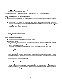
Simulator Console GUI, with the specied system conguration appears on the screen. An example
window is shown in Figure 1.
3
Figure 1: Main Window of the Simulator
Starting a Simulation
To start just rush right into simulating things, the new user can simply hit the "Start" button,
select the "Start w/out recovery le" option, and any of the recovery methods. This causes the
simulator to begin a simulation consisting of the four nodes shown on the console, running a default
static, complex task. The user may use the Schedule, Task Allocation, and Performance buttons to
view the corresponding windows, and watch the simulation progress. A detailed description of other
buttons/commands follows.
2.3 The Console GUI
A Description of the Console and its features and functions is given below. The menu of Main Console
Window is divided into ve subsections: Operation, Conguration, Task Generator, Fault Generator and
Information.
2.3.1 Operation
There are four buttons in the Operation subsection.
4
START is a menubutton with a menu of four options.
{ Start w/o Recovery File is a cascade menu with a submenu listing ve recovery actions, to be
taken in the event that a fault occurs at a particular node. They are: RANDOM, REPLACE,
RETRY REPLACE, DISCONNECT, and RETRY DISCONNECT. A user can select one of
them to start the simulation. When a node fails, the system takes the recovery action, which
has been selected here, to manage failure recovery.
{ Start w/ Building Recovery File is a command menu entry. If a user selects this option, s/he
is prompted to \select a le" from the existing recovery les under directory \data/". The le
selection window is shown in Figure 2. A user can choose a le or input a new lename by
Figure 2: The File Select window for selecting a recovery le
typing its name in the selection Entry or select an existing le by clicking the mouse button-1
on its name in the Listbox. It should be noted that selecting an already existing le causes it
to be overwritten. Once a user hits the key return or the button OK, the dynamic recovery
management algorithm is started. This algorithm takes the current system conguration (from
the le{system.ini) as input and writes the optimal recovery policies into a user chosen le.
When this is done, the simulation is started automatically. During the course of the Simulation,
if a node fails, the system takes the optimal action, provided by the newly generated recovery
le. This Algorithm (RAMP) is discussed in greater detail in section 2.9.
{ Start w/ Existing Recovery Files is a command menu entry. Here, the user is prompted to \select
a le" from the existing recovery les under directory \data/". The user selects a recovery le
5
and the simulation starts immediately. When a node fails, the system takes the optimal action
provided by the selected recovery le.
{ Stop Current Simulation This button is \enabled" only when there is a simulation in progress (or
while one is paused). Pressing it causes the running simulation to be stopped, and the simulator
returned to the state it was in (conguration wise) just prior to its having been \started". The
Recovery Algorithm (RAMP) is discussed in greater detail in section 2.9.
QUIT is a menubutton which can be pressed at any time. The User has two options.
{ Stop Current Simulation This button is identical to the Stop Current Simulation button described above. It is provided in two places in the GUI as a matter of convinence.
{ Quit Simulator Selecting this option quits, entirely, the console GUI, ending any currently
running simulation, and potentially causing unsaved changes to be lost in simulator setups,
taskles and fault les.
PAUSE is a command button which is disabled before the simulation is started. After the simulation
is started, it can be used to pause the simulation (the text and the command associated with this
button are changed from pause to continue) or continue the simulation (the text and the command
are changed back to pause).
CREATE VIEWERS is a menubutton with a menu of a set of names of hosts/displays (from the
le{display.le) This is used for the multiple displays facility. Before the simulation is started, this
button is disabled. Once it becomes normal, a user can select a host/display to create a Viewer GUI
on that terminal. The Viewer GUI contains a limited set of \read-only" functionality and is described
under section 2.4. To ensure that there is only one Viewer GUI created on each host, the selected
display entry is disabled. After the user quits from that Viewer GUI, the menu entry becomes active
again.
LOAD SETUP This button which allows the user to load a setup le, similar to the one which may
be given on the commandline. The user is prompted to select a setup le with which to congure
the simulator, from the \/exe" directory. on the commandline.
SAVE SETUP This button allows the user to save the current setup of the simulator to a le. They
are prompted for a lename to which to save. The le is created, by default, in the \/exe" directory.
2.3.2 Conguration
There are four buttons under Conguration subsection. A user can specify the conguration of the system
by those buttons.
TOPOLOGY is a menubutton with a menu of two entries. Here the user is able to specify the
desired network topology.
{ Fully Connected is a command menu entry. When it is pressed, an \input parameters" window
shown in Figure 3 appears. The user can change the number of virtual nodes and virtual
networks in the simulation. In the current simulator, the number of virtual networks is always
one, regardless of the number entered. Also, in a "fully connected" network, the user has the
option of choosing the network protocol: either FDDI or TOKEN RING.
6
Figure 3: The fully connected topology parameters window
{ Point To Point Connected is a command menu entry. When pressed, the main console window
is changed to a \drawing" window where the user can draw the desired network topology. The
new window that has a dierent set of operational buttons and a blank canvas. Then a user
can draw any point to point topology. This is described in more details under section 2.5.
Each node in the topology graph has a unique node ID and the node with the highest ID number is
always designated to be the master. This is designated with the letter \M". A user can change the
default settings of each node by clicking on the node. A menu is popped up as in Figure 4. Then a
Figure 4: Window for entering node specic parameters - left click on node to view.
user can select the scheduling algorithm(EDF or RATE MONO), whether the node should start o
as a spare node(orange) or an active node(yellow) and on which physical host the node is to be run.
The menu includes the names of the hosts that constitute the PVM virtual machine.
NETWORK PARAMETERS is a button which pulls up a window where the user may specify
a) the length of the ring and b) the distance between nodes. This only applies to the fully connected
topology.
ALLOCATOR is a menubutton with two task allocation algorithms:ROUND ROBIN and UTILIZATION BASED. A user can specify of the allocation algorithms the master uses to allocate tasks
to various active nodes.
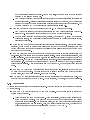
SYSTEM PARAMETERS is a command button. When pressed, a \input system parameters"
window shown in Figure 5 comes up. Here the user can change the parameters of the simulation. The
7
Figure 5: Entering system wide parameters
dierent parameters a user can view are mission time, retry duration, replace duration, disconnect
duration, checkpoint interval, slave alive message interval, and master alive message interval. These
parameters are described in detail in Section 2.7.
2.3.3 Task Generator
There are two buttons under the Task Generator subsection. A user can use these buttons to start the
task editor and specify the tasks that are to be executed during the simulation
TASK EDITOR is a button which brings up a task editor window. The purpose of the window is
so that the user can load, edit and save tasks as well as specify which tasks are run in the simulator.
These tasks may take the form of "real" tasks or static tasks. The Task Editor window is discussed
in detail in section 2.6, along with descriptions of task format and types.
SEND TASK is a command button which is used to send static tasks from the GUI into the
simulated system. This button is only for use while the system is running or paused, and remains
disabled when the simulation is not stopped. The user may "ready" tasks for running with the Task
Editor window, prior to pressing start.
2.3.4 Fault Generator
There are three buttons under Fault Generator subsection. Faults can be injected into and removed from
the system here. The default system is fault free.
INIT FAULT is a menubutton with a menu of four entries. In the simulator, faults are distinguished
as being either transient or permanent. There are two ways by which faults can be injected into the
system. The rst is by specifying the Poisson rates for transient and permanent faults for each node.
The duration in the case of a transient fault must also be specied. The second way is to specify a
8
table of one-time faults for each node. A one-time fault is specied by giving the absolute time at
which a fault must strike the node and the duration of the fault. A -1 value for the duration of the
transient fault indicates that it is eectively a permanent fault. All times are in seconds.
{ TP Faults is a cascade menu entry. When pressed, the user may choose weather or not they
would like to initialize transient or permanent faults. Upon choosing one or the other, a small
\fault editor" window appears where the user may specify the the rate of fault arrivals on a
particular node, and in the case of transient faults, the duration. This window is shown in
Figure 6.
Figure 6: Entering Transient and Permanent Faults
{ One Time Faults Here, the user may choose to initialize faults into the system with a one-time
fault table. The user is prompted to make sure that this is truly their intent. Upon answering
\yes" a \one-time fault editor" appears, and the user is able to specify exact arrival times of
faults on particular nodes, and give the duration of the fault. (-1 indicates a permenant fault.)
An example of this window is shown in Figure 7.
Figure 7: Entering one-time faults
{ Load Faults From Files is a cascade menu with two options: TPFaults and OnetimeFaults. Here
the user may load either type of fault from les.
TPFaults: When it is pressed, a \select a le" window with the existing transient and
permanent fault les(*.t) under the current directory comes up. The user can select a le
to load transient and permanent faults to the system.
9
OnetimeFaults: Its function is similar to TPFaults except it loads one-time faults described
in the selected le(*.ftbl) to the system.
{ Save TPFaults To Files or Save OnetimeFaults To Files is a command menu entry. When it is
pressed, a \select a le" window with the existing transient and permanent fault les(*.t) or
one-time fault les(*.ftbl) under current directory comes up. According to the currently selected
fault type(TPFaults or OnetimeFaults), faults are saved into a user specied le(*.t or *.ftbl).
ADD FAULT is a command button which is disabled before the simulation is started. During the
execution of the simulation, it can be used to open an \Add Onetime Fault" window. The user can
dene a one-time fault by specifying the node on which the fault occurs, the absolute time the fault
must strike the node and the duration of the fault. Click the mouse on the button \SEND" to send
the one-time fault to the system. The absolute time given by user must be greater than the current
time of the central clock.
REMOVE FAULT is a command button which is disabled before the simulation is started. During
the execution of the simulation, it can be used to send clear all faults from a node. Clicking here
sends a nodeId to the system, then the system cleans out all the faults that had been injected into
that node previously.
2.3.5 Information
There are four buttons under Information subsection. These are for opening and closing information
windows which allow the user to track the execution of tasks and the state of the system, during simulation.
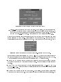
SCHEDULE is a command button which is disabled before the simulation is started. During the
execution of the simulation, this button is used to map or minimize the schedule window which
displays how tasks are scheduled at each node, in real time. Each row represents a node (Y-axis),
with time represented on the X-axis, in seconds. Nodes are identied by number. Tasks scheduled
at a particular node are indicated by color-coded blocks which appear in the row of the node upon
which they are running. The user can see when subtasks are started, when they nish execution,
when they have been preempted or suspended themselves, when they have received/sent messages,
when the nodes have been checkpointed, when faults arrive at a node (its ID becomes red(faulty
node), and nally what kind of recovery action has been taken in case of a fault. It is possible to
remove the information of certain nodes from this window by clicking mouse button-2 on the node ID
and add it back by clicking mouse button-1 on the node square in the main window. The Schedule
window can be scrolled to see the tasks running on all nodes by pressing and holding mouse button-1
and moving the mouse up or down vertically. An example window is shown in Figure 8.
PERFORMANCE is a command button. Before the simulation is started, it yields a menu, so that
a user can select what information is displayed in the system performance window after the simulation
is started. During the execution of the simulation, this button is used to map or minimize the system
performance window. This window gives an overall picture of the simulation in terms of the number
and percentage of: subtasks that have started, subtasks that have nished successfully, subtasks
that have missed their deadline, and subtasks that have been preempted during their execution. An
example window is shown in Figure 9.
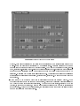
TASK ALLOCATION is a command button which is disabled before the simulation is started.
During the execution of the simulation, this button is used to map or minimize the task allocation
10
Figure 8: Schedule Window of the Simulator
window. This window displays how the tasks have been allocated to the various active nodes by the
master. Each complex task is represented by a particular color. Subtasks belonging to the same
complex task have the same color but a dierent pattern. The window dynamically updates, in realtime, reecting re-allocation of sub-tasks due to faults/failures of nodes. It also shows the utilization
of each node and indicates weather or not there have been any tasks which were not able to be
allocated. (Generally due to insucient resources on nodes. The colors of a node's ID and utilization
reprensentthe node's status: active(yellow), spare(orange), faulty(red). An example window is shown
in Figure 10.
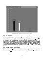
BENCHMARK is a button which maps or minimizes the Benchmark accuracy window. When
the target tracking benchmark is run on the simulator, this window presents a graphical display of
how well the benchmark is tracking it's targets. The number of Real targets, referred to as \Real
Tracks", is shown in the color red, while the benchmarks prediction of the number of real tracks is
shown in green. Where the two colors deviate, the user sees that the benchmark has failed to track
one or more targets to a sucient degree.
11
Figure 9: System Performance Window of the Simulator
2.4 The Viewer GUI
The user can create a Viewer GUI on a particular X-display by clicking on the name of that display under
the button \CREATE VIEWERS". Hosts/Displays listed there are read in from the le: \exe/display.le".
The user may manually edit this le to add/remove displays. Also, the client or destination x-display must
be congured to allow X-connections from the host on which the simulator is running. The Viewer GUI
is similar to the main console window, but has only a limited set of commands. All informational display
screens: schedule window, system performance window, and task table window, can be viewed via the Viewer
GUI. A user can enlarge or shrink these windows, delete a node information from the schedule window and
add it back without aecting other GUIs. The button QUIT may be used at anytime to exit the Viewer
GUI.
2.5 Drawing Point To Point Topology
When a user select Point To Point Topology option under TOPOLOGY, the main window is changed to
a new window that has a new menu(a set of operational buttons) and a blank canvas. Here the user can
draw his own point to point topology on the blank canvas by mouse, or load a previous saved graph to the
12
Figure 10: Task Allocation Window of the Simulator
blank canvas. An example window is shown in Figure 11. Nodes, once placed, may be moved around by
pressing and holding button-2, over a node, and moving the mouse. The functions of the drawing command
buttons are:
ADD NODE is a radio button. When in this mode (it is the default mode) , clicking mouse button-1
on the canvas causes nodes to be added to the topology.
DELETE NODE is a radio button. When in this mode, clicking mouse button-1 on a node causes
the node and any connection lines to the node to be deleted. Other nodes are renumbered accordingly.
CONNECT is a radio button. When in this mode, clicking mouse button-1 on two nodes consecutively causes a connection line to be added between these nodes.
DISCONNECT is a radio button. When in this mode, clicking mouse button-1 on a connection
line cause the connection to be deleted.
DELETE ALL is a command button. When pressed, the entire topology drawn on the canvas is
deleted. Use care and save often!
13
Figure 11: Point to Point Topology
OK is a command button. When pressed, the newly draw topology is retained and control returns
to the Main Console window. (The new topology is not as yet saved, however - the user must save
the topology either with the save button in this window, or by saving the setup in the Main Console)
CANCEL is a command button. When pressed, return to the main window with the original
topology. Any drawn topology is lost.
FILE is a menubutton with a menu of two entries.
{ Load Graph From File: When pressed, a \select a le" window with the existing graph les(*.g)
under current directory comes up. The user can select a graph-le and the graph is drawn on
the canvas.
{ Save Graph as: Its function is similar to Load Graph From File except anything on the canvas
is saved into a user chosen le(*.g).
14
Figure 12: Task Editor Window
2.6 Tasks and the Task Editor Window
The Task Editor allows the user to a) load/save tasks to/from les, b) edit various task parameters c)
specify which tasks are sent to the simulator when the simulation is started. First a word on Tasks and
Task Types.
The term "tasks" refers to the jobs which the simulator either simulates or actually runs. A task of type 3
is known as a static task, where no work or calculation is actually being done, as the task is simulated. A
task of type 5 is know as a "real" task, where actual code is executed in realtime. Right now, there is only
one task of type 5 available to the user, the Benchmark Task, described in section 2.8. Static tasks consist
merely of descriptions of tasks in terms of release time and runtime. Thus, if the user species that a task
should take 5 seconds, the static task uses 5 seconds of CPU time during the simulation. Even though no
real code is executed during that time, the simulated CPU or node is "busy" during that time.
Both types of tasks consist of a two layer hierarchy: Complex tasks, which are composed of subtasks. In
general if several tasks have dependence on one another, the user would probably want to group them
together as subtasks, within the same complex task. Static tasks may be specied, as shown below, with
subtasks that send and receive messages to each other in such a way as to simulate task inter-dependence.
More that one complex task may be run on the simulator at a time.
The task editor window is show below, in Figure 12.
First of all, there are several important buttons in the window.
15
Important Editor Buttons
Load Task Set is a command menu entry. When pressed, a \select a le" window with the existing task
les(*.tsk) under current directory comes up. A user can select a le and load the task description
in this le to the GUI. When loaded, the task(s) appear in the editor, with complex tasks listed by
taskID number. Loading a task set overwrites tasks currently in the editor.
Save Task Set saves all complex and subtasks currently in the editor to a single task description le,
specied by the user.
Add New Task adds a sample complex task to the task set already in the editor. The default task to
be added is specied in the "default.tsk" File.
Add Task From File gives the user the option to choose which task/task set they would like to add
to the current task set by specifying a le from which to load.
Delete Task deletes the complex task or subtask which the user has \highlighted" with their mouse
cursor, in the editor window. If the user tries to delete a subtask with existing dependencies on other
tasks, a warning pops-up.
OK closes the editor window, and retains changes the user has made. Tasks left in the editor at this
point are run when simulation is started. If the user wishes that a task *not* be run, he/she should
save changes and \delete" it.
Cancel closes the editor window without retaining changes to the task set which were initially in the
editor. However, any changes made and saved to disk remain saved.
Editing Tasks
The task editor is provided to give the user a convenient way to modify task parameters online. When
invoked, the \Edit Task Parameters" window appears. Changing the value in the NUM TASKS Entry
changes the number of complex tasks that are sent to the system.
Clicking mouse button-1 on a taskId in the left Listbox of the rst row, all parameters associated with this
complex task are shown in the middle Listbox of the rst row:
TASK TYPE: There are 4 task types: simple aperiodic(0), simple periodic(1), complex aperiodic(2),
complex periodic(3). Currently, only complex periodic(3) is used.
PERIOD INTERVAL: The period of the complex task as a whole.
NUM PERIODS: The number of times that the complex task must be executed. A -1 value indicates
innite number of times or till the end of the mission.
NUM REDUNDANCY: It species the number of nodes on which the same complex task must run.
NEXT RELEASE TIME: It species the time the task must start relative to the start of simulation.
NUM SUBTASKS: It gives the number of subtasks of the complex task. And all subtaskIds of this
complex task are shown in the right Listbox of the rst row.
Clicking mouse button-1 on a subtaskId in the right Listbox of the rst row, all parameters associated with
this subtask are shown in the Listboxes of the second row. An example window is shown in Figure 6.
The parameters shown in the middle Listbox of the second row are:
16
NODEID: It indicates a specic node on which the subtask must run. A -1 value indicates any node.
OFFSET:
EXECTIME: The worst case execution time of the subtask.
DEADLINE: The deadline of the subtask.
PRIORITY: The priority of the subtask.
CHECKPOINT SIZE: the size, in kilobytes of the checkpoints to be taken of this subtask.
NUM RECVMESGS: The number of messages it must receive during its execution.
NUM SENDMESGS: The number of messages it must send during its execution.
The information of the messages that this subtask must receive during its execution are shown in the left
Listbox of the second row. Each line contains the information of a received message which has format:
\FROM taskId subtaskId instanceId AT time". A 0 value in each ID eld means using current task,
subtask or instance, respectively.
The information of the messages that this subtask must send during its execution are shown in the right
Listbox of the second row. Each line contains the information of a sending message which has format:
\TO taskId subtaskId instanceId AT time". A 0 value in each ID eld means using current task, subtask
or instance, respectively.
Clicking mouse button-1 on a parameter of tasks or subtasks, the name and the value of this parameter
are connected with an Entry in this window. Then a user can modify the value in the Entry. Pressing the
key return causes the new value written to the corresponding Listbox.
Press the button OK to exit from the editor.
2.7 Description of System Parameters
These are the Simulation parameters which the user may set or change by using the SYSTEM PARAM-
ETERS button in the main console GUI.
Mission Time is the length, in seconds, of the simulation.
Retry Penalty is the length of time, in seconds, of the "penalty" or "overhead" associated with
performing a Retry recovery action.
Replace Penalty is the length of time, in seconds, of the "penalty" or "overhead" for performing a
Replace recovery action.
Disconnect Penalty is the length of time, in seconds, of the "penalty" or "overhead" of performing a
Disconnect recovery action.
Checkpoint Interval is the interval at which checkpoints are taken of the status of nodes throughout
the simulation.
Slave Alive Mesg. Interval is the interval between "I'm alive" messages from the Slave Nodes.
Master Poll Mesg. Interval is the interval at which the Master Node Polls or Checks its message que
for messages from Slaves.
17
3. Simulation Output Files
When a simulation is run, two output les are created. They are both created in the user's USERDIR/exe,
the directory in which they ran "sim". The rst le, "statle", gives statistics concerning the simulation
run, while the second provides a log le of important events, during the run. Both les are appended to
run after run, so the user may want to make a habit of "mv'ing" each le to another le periodically, or
when an important run has been completed. Output data from seperate runs are delimited in some manner
within the les.
3.1 simstat.dat
This le gives the initial conguration and nal conguration information, as well as a summary of stats
concerning tasks and nodes during the simulation.
Initial Conguration gives a brief overview of the conguration of the simulation, as sent to the master
node at the beginning of the simulation. The initial task set is also documented in this section. Tasks
which have been added to the system manually during runtime are listed at the end of this section.
Final Node Statistics gives an overview of the conguration of the system at the end of the simulation
- ie - when the mission was over or the user pushed the "stop" button. Included are "number of
nodes: alive, dead, spare" and the actual length of simulation. Also included is a "per-node" listing
of "number of tasks: started, nished, missed deadline".
System Task Statistics details the total number of tasks which were started, nished, and "missed
deadline" during the simulation.
3.2 simrun.dat
This File gives a runtime log of events happening during the simulation. It's setup is in intended to provide
a log le which may be monitered during a simulation, and may be parsed easily by shell scripts after the
simulation is over. At the start if each run, the initial conguration is printed to the le. In the "log"
section, here are some of the major events which are displayed.
T ALLOC CHANGE indicates that there has been a change in the allocation of tasks between nodes
(including the initial allocation at the beginning of simulation. All nodes with tasks allocated to
them are printed with this message. Tasks are specied in the form "complexTaskID:subTaskID".
FAULT ARRIVAL and FAULT GONE indicate when a fault has struck a node and when a fault has
"lifted" in the case of transient faults.
RCVRY ACTION indicates when and what recovery action has been taken to recover from a faulty
node.
NOT SPARE and SPARE indicate that a node has either switched from being spare to active or
active to spare.
T CANT START indicates when a complex task can not be allocated due to insucent processor
availability.
18
T MISS indicates that a sub-task has missed its deadline, and tells us which task. Tasks are specied
in the form "complexTaskID:subTaskID".
NEW MASTER indicates that a new master has been elected, generally due to the old master having
failed.
4. The Benchmark Task
The Benchmark Task is a realtime benchmark, originally written by Honeywell Systems, which has been
adapted to run on the Rapids simulator. Setting "Task Type" to 5 causes the simulator to run the
benchmark task.
This is a Target Tracking benchmark, where we are given frames of data, each of which is a eld of
2dimensional data, similar to the output of a radar display. Each contains various "real tracks" and noise
or "false tracks". During runtime, the benchmark attempts to successfully predict which are real, which are
false, and the correct position and velocity of the real tracks. This is done via that "multiple hypothesis"
method.
The user may edit the "Generator inputs.in" le within /usr/local/rapids/rtht bm to change parameter
input to the data generator. The "Objects" correspond to the "real tracks" while, at the bottom of the
le, a number is given for the number of "false tracks" in the system.
When running the benchmark task, the user may click on the "Benchmark" button to view the accuracy
of the benchmark in-terms of number of target successfully tracked and number of targets missed. This is
represented in graphical format.
The user may read a much more detailed description of the benchmark in the Rapids programmers manual.
5. Optimal recovery policy Algorithm - RAMP model
The user can decide if he/she wants to start the simulation with or without making use of the optimal
recovery algorithm policy. If the choice is not to use the algorithm, then either a xed recovery policy or
a random recovery policy can be selected. This is useful for comparing the performance of the algorithm
with xed or random policies.
If the user opts to make use of the algorithm, it is started by selecting 'Start w/ building recovery le'
option from the 'Start' button. Alternatively, if the system parameters are the same as with a previous run
then the simulation can be started with 'Start w/ existing recovery le' option from the 'Start' button. In
this case, the previously created algorithm results le are used and the overhead of running the algorithm
for the same conguration is eliminated.
The simulator provides much of the input to the algorithm. This input consists of several dynamic system
related parameters. Whenever 'Start w/ building the recovery le' option is selected the simulator writes
these parameters into a le named 'system.ini' . The algorithm on starting, then reads and gets its' input
from this 'system.ini' le. The structure of the system.ini le is explained below for a simple system consisting of four nodes:
proc_n
4
num_step 400
T
10000
phases 1
denotes the number of processors (dynamic)
how many steps the mission time is split
denotes the mission time (dynamic)
denotes the number of mission phases (dynamic)
19
C_1_1 125
C_1_2 120
C_1_3 120
the execution time of task 1 assigned to proc. 1 (dynamic)
the execution time of task 2 assigned to proc. 1 (dynamic)
the execution time of task 3 assigned to proc. 1 (dynamic)
D_1_1 250
D_1_2 250
D_1_3 250
the deadline of task 1 assigned to proc. 1 (dynamic)
the deadline of task 2 assigned to proc. 1 (dynamic)
the deadline of task 3 assigned to proc. 1 (dynamic)
R_1 1
the mission phase that the task set is activated (dynamic)
C_2_1 120
C_2_2 120
C_2_3 120
D_2_1 250
D_2_2 250
D_2_3 250
R_2 1
C_3_1 125
C_3_2 120
C_3_3 120
D_3_1 250
D_3_2 250
D_3_3 250
R_3 1
n_ckp
4
number of checkpoints per task execution
tau_rpl
tau_dis
tau_rtr
3
3
1
the replace overhead time (dynamic)
the disconnect overhead time (dynamic)
the retry overhead time (dynamic)
lambda_t_1
lambda_t_2
lambda_t_3
lambda_t_4
3
3
3
3
lambda p_1 1
lambda p_2 0
lambda p_3 0
processor
processor
processor
processor
1
2
3
4
temporary
temporary
temporary
temporary
failure
failure
failure
failure
rate
rate
rate
rate
(dynamic)
(dynamic)
(dynamic)
(dynamic)
processor 1 permanent failure rate (dynamic)
processor 2 permanent failure rate (dynamic)
processor 3 permanent failure rate (dynamic)
20
lambda p_4 0
processor 4 permanent failure rate (dynamic)
out_file data/try
name of output data file
The elds which depend on the characteristics of the system being simulated are denoted as dynamic elds.
The most important non-dynamic parameter is the num steps parameter. The mission time is split into
num steps number of steps and reliability is computed for each step. Therefore increasing this parameter
increases the accuracy of the optimal recovery algorithm but also increases the running time.
Increasing the permanent error rate biases the algorithm towards a replace/disconnect action whereas
increasing the temporary error rate biases it towards a retry action.
Decreasing an action overhead also biases the algorithm towards that particular action.
In the simulator some tasks can have non-zero phasing times. However, once started, tasks run until the
end of the mission. Therefore the overall system load can only increase. If some tasks have non-zero
phasing, then the time they are phased in is considered as the start of a new mission phase. The algorithm
is repeated for each phase with the only change being the overall load.
21