Download Measurement of changing mechanical properties of carbon

CZECH TECHNICAL UNIVERSITY IN PRAGUE
ČESKÉ VYSOKÉ UČENÍ TECHNICKÉ V PRAZE
FACULTY OF ELECTRICAL ENGINEERING
DEPARTMENT OF MICROELECTRONICS
FAKULTA ELEKTROTECHNICKÁ
KATEDRA MIKROELEKTRONIKY
MEASUREMENT OF CHANGING MECHANICAL
PROPERTIES OF CARBON COMPOSITE ON
NANOSATELLITE MINICUBE MISSION QB50
MASTER’S THESIS
DIPLOMOVÁ PRÁCE
2015
Bc. ONDŘEJ NENTVICH
CZECH TECHNICAL UNIVERSITY
IN PRAGUE
ČESKÉ VYSOKÉ UČENÍ TECHNICKÉ V PRAZE
FACULTY OF ELECTRICAL ENGINEERING
DEPARTMENT OF MICROELECTRONICS
FAKULTA ELEKTROTECHNICKÁ
KATEDRA MIKROELEKTRONIKY
MEASUREMENT OF CHANGING MECHANICAL
PROPERTIES OF CARBON COMPOSITE ON
NANOSATELLITE MINICUBE MISSION QB50
MĚŘENÍ ZMĚN MECHANICKÝCH VLASTNOSTÍ UHLÍKOVÉHO KOMPOZITU NA
NANOSATELITU MINICUBE MISE QB50
MASTER’S THESIS
DIPLOMOVÁ PRÁCE
AUTHOR
Bc. ONDŘEJ NENTVICH
AUTOR PRÁCE
SUPERVISOR
Ing. LADISLAV SIEGER, CSc.
VEDOUCÍ PRÁCE
Prague
2015
České vysoké učení technické v Praze
Fakulta elektrotechnická
katedra mikroelektroniky
ZADÁNÍ DIPLOMOVÉ PRÁCE
Student:
Bc. N E N T V I C H Ondřej
Studijní program:
Obor:
Komunikace, multimédia a elektronika
Elektronika
Název tématu:
Měření změn mechanických vlastností uhlíkového kompozitu na
nanosatelitu miniCube mise QB50
Pokyny pro vypracování:
1) Prostudujte problematiku vyhodnocení útlumu exponenciálně tlumeného signálu
vznikajícího kmitáním uhlíkového kompozitu
2) Navrhněte algoritmus vyhodnocení útlumu měřeného signálu
3) Prostudujte vhodné způsoby excitace uhlíkového kompozitu a snímání jeho kmitů
4) Navrhněte systém pro měření změn mechanických vlastností uhlíkového kompozitu
v závislosti na změně teploty
5) Relizujte vhodné zapojení z 3) a 4) pro Payload nanosatelitu miniCube mise QB50
6) Realizujte měření pod systémem RTOS
7) Ověřte a zhodnoťte funkčnost systému
Seznam odborné literatury:
[1] JAN, J. Číslicová filtrace, analýza a restaurace signálů. 2nd ed. Brno: VUTIUM, 2002. 427
p. ISBN 80-214-2911-9
[3] TŮMA, J. Zpracování signálů získaných z mechanických systémů užitím FFT. Praha:
Sdělovací technika, 2000. 168 p. ISBN 80-901936-1-7
[3] HANA, P., INNEMAN, A., DANIEL, V., et al. Mechanical properties of Carbon Fiber 3
Composites for applications in space. Proc. SPIE 9442, Optics and Measurement
Conference 2014, 2015, , no. 1, DOI: 10.1117/12.2175925
Vedoucí:
Ing. Ladislav Sieger, CSc.
Platnost zadání:
31. 8. 2016
L.S.
prof. Ing. Miroslav Husák, CSc.
vedoucí katedry
V Praze dne 16. 2. 2015
prof. Ing. Pavel Ripka, CSc.
děkan
Czech Technical University in Prague
Faculty of Electrical Engineering
Department of Microelectronics
Master’s Thesis Assignment
Student:
Bc. N E N T V I C H
Ondřej
Study program:
Focused:
Communication, Multimedia and Electronics
Electronics
Topic:
Measurement of changing mechanical properties of carbon composite on nanosatellite
miniCube mission QB50
Instructions:
1) Study the problematic of evaluating the attenuation of exponentially attenuated
signal generated by oscillations of carbon composite.
2) Implement an algorithm to evaluate the attenuation of the measured signal.
3) Study the suitable methods of excitation of the carbon composite and sensing its
oscillations.
4) Design a system for measurement of mechanical changes of the carbon composite
in dependence on the temperature change.
5) Implement a suitable wiring from 3) and 4) for the Payload of nanosattelite
miniCube mission QB50.
6) Implement the measurement under the RTOS system.
7) Check and evaluate the functionality of the system.
References:
[1] JAN, J. Číslicová filtrace, analýza a restaurace signálů. 2nd ed. Brno: VUTIUM, 2002.
427 p. ISBN 80-214-2911-9
[2] TŮMA, J. Zpracování signálů získaných z mechanických systémů užitím FFT. Praha:
Sdělovací technika, 2000. 168 p. ISBN 80-901936-1-7
[3] HANA, P., INNEMAN, A., DANIEL, V., et al. Mechanical properties of Carbon Fiber 3
Composites for applications in space. Proc. SPIE 9442, Optics and Measurement
Conference 2014, 2015, , no. 1, DOI: 10.1117/12.2175925
Supervisor:
Ing. Ladislav Sieger, CSc.
Assignment validity:
31. 8. 2016
L.S.
prof. Ing. Miroslav Husák, CSc.
prof. Ing. Pavel Ripka, CSc.
Head of department
Dean
In Prague, 16. 2. 2015
ABSTRACT
ANOTACE
This master’s thesis talking about measurement of mechanical changes of carbon fibre material. The board is one
of the part nanosatellite VZLUsat-1 and
one of experiments on board. Microcontroller processing sampling of signal,
calculates Fast Fourier Transform and
attenuation of signal. All measurements
of the probe VZLUsat-1 will be launched
during mission QB50.
Tato diplomová práce pojednává
o měření mechanických vlastností
uhlíkového kompozitu. Měřící deska je
jednou z mnoha dalších na nanosatelitu
VZLUsat-1 a jednou z experimentů.
Mikrokontrolér zpracovává navzorkovaný signál, spočítá rychlou Fourierovu
transformaci a útlum signálu. Veškerá
měření na sondě VZLUsat-1 budou
vypuštěna během mise QB50.
KEYWORDS
KLÍČOVÁ SLOVA
QB50, CubeSat, Space, FFT, Composite, Carbon, VZLUSAT1, Sampling, Research
QB50, CubeSat, Vesmír, FFT, Kompozit, Carbon, VZLUSAT1, Vzorkování,
Výzkum
NENTVICH, Ondřej. Measurement of changing mechanical properties of carbon composite on nanosatellite miniCube mission QB50: master’s thesis. Prague: Czech Technical University in Prague, Faculty of Electrical Engineering, Department of Microelectronics, 2015. 75 p. Supervised by Ing. Ladislav Sieger, CSc.
VII
ACKNOWLEDGEMENT
DECLARATION
I would like to express thanks to the
mentor Mr. Ing. Ladislav Sieger, CSc.
for many useful advices, comments and
patience during works on nanosatellite,
this master’s thesis and also to my colleagues who support me.
Also I would like to express huge gratitude to Mr. Kazuo Yana, Ph.D. from
Hosei University in Tokyo, Japan, who
provided me experiences about signal
processing during summer internship in
2014.
I declare that I have written my master’s thesis on the theme of “Measurement of changing mechanical properties of carbon composite on nanosatellite miniCube mission QB50” independently, under the guidance of the master’s thesis supervisor and using the
technical literature and other sources of
information which are all quoted in the
thesis and detailed in the list of literature at the end of the thesis.
As the author of the master’s thesis I furthermore declare that, as regards the creation of this master’s thesis, I have not infringed any copyright.
In particular, I have not unlawfully encroached on anyone’s personal and/or
ownership rights and I am fully aware of
the consequences in the case of breaking
Regulation S 11 and the following of the
Copyright Act No 121/2000 Sb., and of
the rights related to intellectual property right and changes in some Acts (Intellectual Property Act) and formulated
in later regulations, inclusive of the possible consequences resulting from the
provisions of Criminal Act No 40/2009
Sb., Section 2, Head VI, Part 4.
In Prague,
July 30, 2015
.....................................
author’s signature
IX
Contents
4.6
List of Figures
XIII
List of Tables
XV
List of Codes
How to Excite the
Cantilever . . . . . . .
4.7 HM Panel . . . . . . .
4.8 Measured Parameters .
4.8.1 Young’s Modulus
of Elasticity . .
4.8.2 Attenuation of
Signal . . . . .
4.9 Computing Process of
FFT . . . . . . . . . .
4.10 Computing Process of
Attenuation . . . . . .
4.10.1 Rectify
and
Moving Averages
4.10.2 Logarithm
Moving Averages
4.10.3 Least Square .
XVII
List of Acronyms
XIX
List of Symbols
XXI
1 Introduction
1
2 Mission QB50
2.1 One CubeSat unit . . .
3
3
3 CubeSat VZLUsat-1
5
3.1 Parts of Probe . . . . .
6
3.1.1 X-Ray Optics
and Medipix . .
6
3.1.2 Radio . . . . .
7
3.1.3 Scientific Unit .
7
3.1.4 Volatiles Board
7
3.1.5 Radiation
Shielding
Measurement .
8
3.1.6 HM System . .
8
3.1.7 On
Board
Computer . . .
8
3.1.8 Electronic
Power System .
9
3.1.9 Stabilising system 9
5 Device for Mechanical
Changes Measurement
5.1 HM panel . . . . . . .
5.2 HM board . . . . . . .
5.2.1 Microcontroller
for Payloads . .
5.2.2 Oscillator . . .
5.2.3 External Memory
5.2.4 Power Switch .
5.2.5 Piezo Connection
5.2.6 Thermometer .
6 Communication
with
Other Boards
6.1 I2 C Interface . . . . . .
6.2 CubeSat Space Protocol
6.3 FreeRTOS . . . . . . .
6.3.1 Creating Tasks
6.4 Communication with
HM Board . . . . . . .
6.4.1 Measure Starts
4 Mechanical
Changes
Measurement
11
4.1 Damped Oscillations . 11
4.2 Elementary Oscillator . 13
4.3 Cantilever Oscillations
13
4.4 Measuring by Accelerometer 15
4.5 Measuring by Piezo . . 15
XI
16
16
16
17
17
18
20
21
22
22
25
25
27
27
28
29
29
30
31
33
33
34
35
35
36
37
6.4.2
6.5
Returns Signal
to DK . . . . . 37
6.4.3 Returns Results
of Measurement 37
6.4.4 Returns Temperature
of HM Board . 37
Data Keeper . . . . . . 38
7 Measurement Process in
HM board
7.1 Read Parameters of
Measurement . . . . .
7.2 Get
Temperature,
Orientation and Time .
7.3 Excite of Coil and
Sampling of Signal . .
7.4 Signal Processing – FFT
7.4.1 Decimation
and
Address
Bit Reversing .
7.4.2 FFT Process .
7.5 Signal Processing –
Attenuation . . . . . .
7.6 Store Results . . . . .
7.7 Conclusion . . . . . . .
8 Measurements,
Testing
and Results
8.1 Beginning of Research
8.2 Research
During
Internship in Japan . .
8.3 Testing of Pulse Width
8.4 Different
Climate
Conditions . . . . . . .
8.5 Final Implementation .
8.6 Final Measurements
Before Flight . . . . .
8.7 Conclusion . . . . . . .
9 Conclusion
39
39
40
41
41
41
43
44
45
45
47
48
49
50
51
54
54
56
57
XII
References
59
List of appendices
63
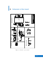
A Schematic of the board
65
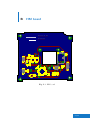
B HM board
67
C Article from Japan
69
D Content of DVD
75
List of Figures
8.5
3.1
Nanosatellite VZLUsat-1 .
4.1
Picture of elementary
damped oscillator . . . . .
11
4.2
Simulated damped signal .
12
4.3
Length of string L vs.
wavelength 𝜆 . . . . . . .
13
4.4
Picture of the Cantilever .
14
8.9
4.5
Drawings
of
Health
Monitoring (HM) panel . .
17
8.10
4.6
Sample of signal . . . . . .
18
4.7
Flowchart of computing
FFT with N=16 points . .
19
4.8
Detail of a butterfly . . .
19
4.9
Result of moving averages
21
4.10 Attenuation with directive
22
5.1
Picture of HM panel . . .
25
5.2
Detail of HM panel . . . .
26
5.3
Picture of HM board with
highlighted parts . . . . .
27
5.4
Schematic of power switch
29
5.5
Schematic
of
piezo
connection . . . . . . . . .
30
Schematic of connection
I2 C devices [19] . . . . . .
33
Chart with communication
via I2 C [19] . . . . . . . .
34
6.3
CSP header . . . . . . . .
34
8.1
Difference in spectra with
different placement . . . .
47
Differences in spectra
without and with using
FIR filter . . . . . . . . .
48
Photo of development kit
[24] . . . . . . . . . . . . .
49
Signal with triangular
envelope . . . . . . . . . .
50
6.1
6.2
8.2
8.3
8.4
5
8.6
8.7
8.8
A.1
B.1
B.2
XIII
Differences between pulse
widths . . . . . . . . . . .
Chart of different climate
conditions . . . . . . . . .
Signal level comparison at
different temperatures . .
Spectrum comparison at
different temperatures . .
Histograms of natural
frequencies . . . . . . . . .
Chart of temperature and
attenuation in time . . . .
Schematic of power switch
HM board . . . . . . . . .
Dimensions of HM board .
51
51
52
53
55
55
65
67
68
List of Tables
3.1
4.1
4.2
5.1
5.2
6.1
6.2
8.1
Scientific units [3] . . . . .
Cantilever Parameters . .
Bit reversing . . . . . . .
Parameters of MCU
ATxMega128A4U [15] . .
Parameters of thermometer
ADT7420 [18] . . . . . . .
xTaskCreate Command
Parameters [22] . . . . . .
Communication ports of
HM board . . . . . . . . .
Searching ranges of peaks
in the spectrum . . . . . .
7
15
19
28
31
36
37
53
XV
List of Codes
6.1
6.2
7.1
7.2
7.3
7.4
7.5
Main loop of any task . .
Respond to Get Temperature Command . . . . . .
Parameters of Measurement
Decimation and bit reversing
Calculation of FFT . . . .
Calculation of attenuation
Output structure . . . . .
36
38
40
42
43
44
46
XVII
List of Acronyms
ACK
Acknowledge
FIR
Finite impulse response
ADC
Analog to Digital Converter
Flash
Type of non-volatiles memory
CMOS
Complementary
Metal-Oxide-Semiconductor
FRAM
Type of non-volatiles memory
FreeRTOS
Free Real Time Operating
System
CSP
CubeSat Space Protocol
CubeSat
Small standard nanosatellite
of dimensions 10x10x10 cm
per unit
FW
Firmware
DFT
Discrete Fourier Transform
HM
Health Monitoring
DiF
Decimation in frequency
HW
Hardware
DiT
Decimation in time
I/O
Input/Output
DK
Data Keeper
I2 C
Inter-Integrated Circuit
DSP
Digital Signal Processing
INMS
Ion-Neutral Mass
Spectrometer
HK
House keeping
EEPROM
Type of non-volatiles memory
LCD
Liquid crystal display
EPS
Electrical Power System
LED
Light emitting diode
etc.
etcetera
LHC
Large Hadron Collider
FEM
Finite element method
m-NLP
multi-Needle Langmuir Probe
FFT
Fast Fourier Transform
MCU
Microcontroller
FIPEX
Flux-Φ-Probe Experiment
XIX
MOSFET
Metal Oxide Semiconductor
Field Effect Transistor
VZLÚ
Výzkumný a zkušební letecký
ústav, a.s. – Aerospace
Research and Test
Establishment
NACK
No Acknowledge
OBC
On Board Computer
PC
Personal computer
ppm
points per million
QB50
Missions of nanosatellites
CubeSats
RAM
Type of volatiles memory
SCL
Serial clock
SD
Secure digital
SDA
Serial data
SPI
Serial Peripheral Interface
SRAM
Type of volatiles memory
USART
Universal synchronous and
asynchronous serial receiver
and transmitter
vs.
versus
VZLUsat-1
Marking of nanosatellite from
institution VZLÚ
XX
List of Symbols
𝐴
Cross
sectional area
(︁ )︁
2
m
𝐸
𝐹d
𝐹i
𝐹r
𝐽
𝑁
𝑁
𝛽𝑛
𝜔𝑛
Elastic Modulus
(Pa)
Angular frequencies of
natural
oscillations
(︁
)︁
−1
rad · s
𝜌
Damping force
(N)
Material
Density
(︁
)︁
−3
kg · m
𝑏
Inertial force
(N)
Cantilever width
(m)
𝑐0
Reverse force
(N)
Velocity
of longitudinal waves
(︁
)︁
−1
m·s
𝑓dec
Decimated frequency
(Hz)
Quadratic
torque-section
(︁ )︁
4
m
𝑓max Maximal frequency
(Hz)
Number points of signal
(−)
Number of point least square
method
(−)
Own root of frequency
equation
𝑓s
Sampling frequency
(Hz)
ℎ
Cantilever height
(m)
𝑗
Quadratic sectional radius
(m)
𝑘
Number points of moving
averages
(−)
𝛿
Attenuation
of system
(︁
)︁
−1
s
𝜆
Wavelenght
(m)
𝑘
Directive of line
(−)
𝜔
Angular
frequency
(︁
)︁
rad · s−1
𝑘
Spring
constant
)︁
(︁
N · m−1
𝜔0
Angular frequency of natural
oscillations
(︁
)︁
rad · s−1
𝑙
Cantilever length
(m)
𝑚
Mass
(kg)
XXI
𝑞
Offset of line
(dB)
𝑣
Velocity
of propagation
(︁
)︁
−1
m·s
𝑥
Point of signal
(mV)
𝑥
Deviation
(m)
𝑥i
Time point in least square
method
(s)
𝑦i
Amplitude point in least
square method
(dB)
XXII
1
Introduction
This master’s thesis is generally talking about mission QB50, small nanosatellites
called CubeSat. Main part of the thesis is measuring mechanical changes of carbon
fibre material in time. It seems to be quite easy task, but there are many aspects
which could happened and all dangerous states that must be prevented. So here is a
reason to test all climatic conditions, mainly in vacuum and operation temperatures
on orbit.
The probe also has many other measurements such as X-Ray measurement of
the Sun called Medipix, evaporation measurement, verifying quality of the carbon
fibre shielding and some other measurements. For example issue of evaporation is
detailed and described in the thesis Measurement of evaporation and evaluation of
changes of the mechanical properties of carbon composite on nanosatellite miniCube
mission QB50 [1] of my colleague Bc. Martin Urban. Or the issue with radiation
shielding has in charge my other colleague Bc. Veronika Stehlíková and it is more
detailed in her thesis Radiation resistance measurement on nanosatellite miniCube
mission QB50 [2].
Tested carbon fibre material could be used on a new satellites in future and it
should replace old and heavy tungsten shielding. It would lead to decrease in weight
of the whole satellite and launch cost.
The device for measuring mechanical changes in time consists of excitation coil
which attracts cantilever with glued permaloy circle. It causes vibrations of the
beam and produce mechanicaly damped oscillations which are measured by piezoelectric element. Piezo transforms mechanical oscillations into electrical. Then
Microcontroller samples them and evaluate them. Process of evaluation consists of
calculation of Fast Fourier Transform (FFT) and attenuation of the signal. Results
of the measurement are frequencies, one is mechanical resonance of the beam, the
other frequencies are resonances of whole satellite and the last measured parameter
is attenuation of beam for additionally specifying of the model using Finite element
method (FEM).
Measurement board runs under Free Real Time Operating System (FreeRTOS)
and communicates with the probe through CubeSat Space Protocol (CSP) via InterIntegrated Circuit (I2 C) interface.
1/75
2
Mission QB50
Main idea of the mission QB50 is that anybody could build their own probe
especially Universities with quite low-cost start and required equipment. Basic cost
for Hardware (HW) is in range 50-100 thousands Euro. Name QB50 is derived from
number of CubeSats.
Generally 50 CubeSats are carried out on orbit. These probes are from whole
the world. One of them is Czech nanosatellite VZLUsat-1 which is the first probe
that will be launched during mission QB50.
Each satellite is normalized to units which must be observed. Basic idea of the
mission QB50 is discovering the least explored lower thermosphere – measuring or
research in these altitudes about 200-380 km.
Launch is scheduled on February 1, 2016 from Alcantara launch site in Brazil by
rocket Cyclone-4 [3].
2.1
One CubeSat unit
One unit of the probe has these parameters [3]:
• Dimmensions 10 × 10 × 10 cm per unit
• Weight up to 1 kg per unit
• Units up to 3 units in row (30 × 10 × 10 cm), during this mission
Advantages of CubeSats are that existing standardised HW boards like On Board
Computer (OBC), Electrical Power System (EPS) board, solar panels, radio board,
etc. are qualified for these missions and use in space environment. It is only necessary to implement communication with other boards [4].
3/75
3
CubeSat VZLUsat-1
(a) Picture of deployed satellite
(b) Measurements on satellite
Fig. 3.1: Nanosatellite VZLUsat-1
One of the Czech nanosatellites is VZLUsat-1 shown in Fig. 3.1a. Výzkumný a
zkušební letecký ústav, a.s. – Aerospace Research and Test Establishment (VZLÚ)
is supervisor and main coordinator of project and it has whole team participating
on the probe. The team involves some universities and companies such as Czech
Technical University in Prague, University of West Bohemia, Rigaku Innovative
Technologies Europe, TTS, 5M, IST, . . .
Probe VZLUsat-1 consists of many experiments as is shown in Fig. 3.1b. One
of them is X-Ray camera called Medipix with Lobster Eye (X-Ray) optics with
focal length approx. 20 cm. It takes pictures of the Sun and measures X-ray intensity in range 5-20 keV. The important thing is measuring of temperature. Satellite
5/75
3. CubeSat VZLUsat-1
have many PT1000 temperature sensors connected to the one common board called
Measure Board. Another measurement is HM system which consists of measuring
mechanical changes in time, radiation shielding and evaporation from the carbon
fibre on the probe. The goal is to verify properties of carbon fibre material in space.
Dimensions of the probe in packed state are 20×10×10 cm and when VZLUsat-1
will be dropped out from launcher with other satellites then it deploys solar panels,
Lobster Eye optics and HM panel. Dimensions will change to approx. 30×10×10 cm.
Unpacked state is in the picture Fig. 3.1a.
3.1
Parts of Probe
Each member of the team is responsible for specific part of scientific experiment
on board. The most important parts are on the followings pages. Almost all boards
are connected through main 80 pins connector which contains power, reserved data
signals and also user defined pins which could be used for any purpose.
3.1.1
X-Ray Optics and Medipix
Probe VZLUsat-1 has X-Ray optics with focal length approx. 20 cm and should
be looking into the Sun. This state will happened twice a year because of static
orientation of probe. For detection of the right orientation there are three sensors,
two in UV spectrum and one in IR spectrum. Main reason why probe has two UV
diodes is that one is sensitive in maximum radius approx. 80°, second one has radius
reduced to approx. 15° by a small tube. The first one is looking for sources of UV
radiation, mainly from the Sun in wide angle and the second one has narrower angle
for more precise determination of Sun position. When both sensors have strong
enough UV signal then Medipix will start up, which then take a picture of the Sun.
Medipix is CMOS silicon detector originally developed as low energy (1 – 20 keV)
X-Ray detector for Large Hadron Collider (LHC) in CERN. Board with this chip
assembled on the probe was used as medical equipment for scanning soft tissues with
high resolution. For this mission Medipix/Timepix is used for detection X-Rays from
the Sun [5].
6/75
3.1 Parts of Probe
3.1.2
Radio
Radio is one of the most important boards on every satellite. It provides communication between Earth and downloading results or uploading configurations.
Transmission frequency is in radio-amateur free band at 436 MHz with communication speed 9 600 Baud.
University of West Bohemia is responsible for communication with the sat. They
will download data and upload configurations to the probe. And also process some
data from it. Communication board which will be launched, is already tested with
antenna and radio board and works fine on the ground in 10 km distance [6].
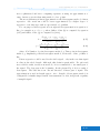
3.1.3
Scientific Unit
Every nanosatellite should have one of three scientific units:
Tab. 3.1: Scientific units [3]
Type
Description
INMS
FIPEX
m-NLP
Ion-Neutral Mass Spectrometer
Flux-Φ-Probe Experiment
multi-Needle Langmuir Probe
All scientific units are equipped with a thermometer such as Thermistor, Thermocouple, . . .
VZLUsat-1 has FIPEX as scientific unit. The unit measures behaviour of atmospheric oxygen at lower thermosphere. It is important for exploring erosion on
surfaces of spaceships during contact of atomic oxygen with surface of probes [3, 7].
3.1.4
Volatiles Board
Volatiles board is assembled with humidity sensors which are looking for residual
humidity or evaporation from the whole probe, mainly from carbon-fibre materials.
It has three types of sensors, two from IST company labeled HYT271 and HYT939,
both in two of each. Third type is HAL2 in three pieces from TTS company. It is
not only sensitive to humidity, but a little to other gases. All sensors are connected
to the board with a driver called PicoCap which is converting capacitance into ratio
compared to the reference capacitance. All HYT sensors and PicoCap communicate
7/75
3. CubeSat VZLUsat-1
via I2 C bus connected directly to the OBC. Everything about humidity sensors and
measuring evaporation is described in detail in thesis of my colleague Martin Urban
in [1].
3.1.5
Radiation Shielding Measurement
The goal of this experiment is to verify quality of radiation shielding of Carbonfibre composite using three same XRB diodes. One is looking into the space, second
is covered by this material and third is shielded by composite and by tungsten sheet.
Evaluation of shielding quality is comparing all three diodes together. First
serves reference for maximal intensity of radiation, middle diode real intensity of
radiation and third is measuring background. This issue is described in more detail
in thesis of my colleague Veronika Stehlíková in [2].
3.1.6
HM System
Health Monitoring system contains two parts. One is mechanical part with
beam made of carbon-fibre composite and six thermometers PT1000. Thermometers
measure heat transmission from one surface to another and how good reflectivity
of thermal radiation surface layers of Nickel or Gold is. Also HM panel measures
aging of carbon-fibre material using excitation of beam and measure its oscillations
by piezo. Whole signal is sampled by ADC in MCU. Microcontroller is on the HM
board which is the second part of Health Monitoring system. Evaluation of signal
is done by FFT and results are resonant frequencies of beam and of the probe. This
issue is described in more detail on followings pages of this thesis.
3.1.7
On Board Computer
On Board Computer is synonymous for heart of probe. Board is in charge of
many functions, but primary is operating other boards, their requirements and reply
to them. Besides that, it communicates with ground segment and organizing further
actions on the deck.
8/75
3.1 Parts of Probe
3.1.8
Electronic Power System
Power system consists of solar panels which generate electric energy and power
board which transforms and stabilizes voltage at defined value (5 V or 3.3 V). Board
has two backup lithium batteries when probe is in solar shade. This board is autonomous and when power goes under critical value, it cuts off all systems included
OBC and then it waits for power.
3.1.9
Stabilising system
It is necessary to stabilize probe to its defined state. Small nanosatellites does
not have rockets for stabilization, but it has six coils – two in each dimension. Coils
are excited by electric pulses and create the force necessary to stabilize the probe
according to magnetic field of Earth.
9/75
4
Mechanical Changes Measurement
Main part of this thesis is about measuring mechanical changes. Here, on a few
pages in this chapter, is described theory about measurement of mechanical changes
– equations how to compute natural frequencies in the elementary case as a string,
or for the real model of a cantilever with one fixed side. It is also described how to
get the natural frequencies from sampled signal – by using FFT. It is supposed that
the cantilever produces damped oscillations with exponential envelope and signal is
then analysed by linear regression. All these processes are discussed on the following
pages.
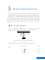
4.1
Damped Oscillations
Damped oscillator is in the illustration Fig. 4.1 with spring which is represented
by Spring constant (𝑘), weight at the end by Mass (𝑚) and deviation by 𝑥.
x
k
m
Fig. 4.1: Picture of elementary damped oscillator
These oscillations could be described using following equation (4.1).
𝐹f + 𝐹d + 𝐹r = 0
(4.1)
where
d2 𝑥
d𝑡2
d𝑥
𝐹d = 𝑏
d𝑡
𝐹r = 𝑘𝑥
𝐹f = 𝑚
(4.2)
(4.3)
(4.4)
11/75
4. Mechanical Changes Measurement
and meaning Inertial force (𝐹i ), Damping force (𝐹d ), Reverse force (𝐹r ).
When equations (4.2 – 4.4) are put into (4.1), it gets differential equation of
second order (4.5).
d2 𝑥
d𝑥
+ 𝑘𝑥 = 0
+𝑏
2
d𝑡
d𝑡
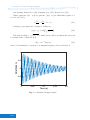
Solving it, gets equation for damped oscillations
(4.5)
𝑚
𝑥(t) = 𝑥0 𝑒
−𝛿𝑡
(︂ √︁
sin 𝑡
𝜔02
−
𝛿2
)︂
(4.6)
√︁
If it is known that 𝜔 = 𝜔02 − 𝛿 2 , formula (4.6) could be rewritten into the form
for damped sine oscillations (4.7).
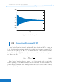
𝑥(t) = 𝑥0 𝑒−𝛿𝑡 sin (𝜔𝑡)
(4.7)
where 𝛿 is Attenuation of system, 𝜔 is Angular frequency and 𝑥 is Deviation.
1
Amplitude (-)
0.5
0
-0.5
-1
0
0.05
0.1
0.15
Time (s)
Fig. 4.2: Simulated damped signal
12/75
0.2
4.3 Cantilever Oscillations
4.2
Elementary Oscillator
Elementary oscillator could be described on simplified example as a string. In
this case the following equation (4.8) for examination Young’s modulus of elasticity
is applied.
√︃
𝑣=
𝐸
𝜌
(4.8)
where Velocity of propagation (𝑣) is defined as 𝑣 = 𝜆𝑓 , 𝜆 is Wavelenght, 𝐸 is
Elastic Modulus, 𝜌 is Material Density.
In this case it is possible to determine that 𝜆 = 4𝐿, where L is part of string
length illustrated in Fig. 4.3.
λ
L
Fig. 4.3: Length of string L vs. wavelength 𝜆
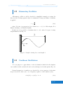
4.3
Cantilever Oscillations
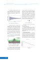
For our purpose to approximate to the real situation which is in the simplest
case cantilever with one fixed side and one freely hanged, as is in the picture Fig. 4.4.
Natural frequencies of cantilever are described by a few equations. In the first
step it is needed to find own roots of frequency equation of the cantilever (4.9).
cosh (𝛽𝑛 𝑙) · cos (𝛽𝑛 𝑙) + 1 = 0
(4.9)
13/75
4. Mechanical Changes Measurement
l
b
Fig. 4.4: Picture of the Cantilever
This equation can be solved only by numeric method and its four first roots are:
𝛽1 𝑙 = 1.875
𝛽2 𝑙 = 4.694
𝛽3 𝑙 = 7.855
𝛽4 𝑙 = 10.996
where 𝛽𝑛 is Own root of frequency equation, 𝑙 is Cantilever length [8].
Natural frequencies are computed using following equation (4.10). For this formula it is required to know computed roots and some other parameters, all necessities
are in Tab. 4.1 and put into equation (4.11).
𝛺n =
(𝛽n 𝑙)2
𝑐0 𝑗
𝑙2
(𝛽n 𝑙)2
Ωn =
𝑙2
√︃
(𝛽n 𝑙)2
=
𝑙2
√︃
𝐸
𝜌
√︃
𝐸
𝜌
√︃
(4.10)
𝐽
=
𝐴
(4.11)
ℎ2
12
(4.12)
where 𝑗 is Quadratic sectional radius, 𝑐0 is Velocity of longitudinal waves, 𝐽 is
Quadratic torque-section and 𝐴 is Cross sectional area.
Conversion between angular speed and frequency is in following equation (4.13).
𝑓=
14/75
Ωn
2𝜋
(4.13)
4.5 Measuring by Piezo
Tab. 4.1: Cantilever Parameters
Symbol
𝑙
𝑏
ℎ
𝐸
𝜌
Description
Cantilever length
Cantilever width
Cantilever height
Elastic Modulus
Material Density
Investigated parameter is Young’s modulus of elasticity 𝐸 and it is verified using
formula (4.11). From this point of view, it is a prerequisite that the other parameters
do not change according to Tab. 4.1.
Properties of cantilever could be also simulated using FEM. This issue was simulated by Petr Hána from Technical University of Liberec using FEM and results of
this method were almost the same as using equation (4.11) [8–10].
For verifying natural frequencies, it is needed to get oscillations from the beam.
Signal measurement could be performed by two methods. One is by accelerometer
and another one is by piezoelectric plate.
4.4
Measuring by Accelerometer
Accelerometers are usually small and lightweight, about a few grams. One
disadvantage is that they must be placed into position with the highest variation of
signal – for the highest acceleration. That location is at the end of the cantilever. It
is not recommended for this purpose because the weight of the plate is about a few
grams and accelerometer with wires would cause bigger attenuation and frequency
change. Results of measured cantilever would be changed – there would be a big
deviation from theoretical results [10].
4.5
Measuring by Piezo
Another method how to measure oscillations is by piezoelectric plate. Here are
some requirements for placing it for higher sensitivity and it is the place with the
mechanical stress of the measured material and that position is at a fixed end of
15/75
4. Mechanical Changes Measurement
cantilever. When piezo is stressed, it produces electrical voltage which is measured,
it corresponds to mechanical oscillations in this case [10].
4.6
How to Excite the Cantilever
Here is another issue and it is how to excite the cantilever. One of the possibilities is to tap it by finger, but it is not suitable for autonomous measurement or in
space. There are some other possibilities and one of them is to mechanically tighten
the cantilever and then let it go. This situation is not reliable from my point of
view. There should be a precise mechanism.
There is another method and it is electrical excitation of beam. At the opposite
side of the cantilever is a fixed coil which attracts the beam by electric pulse to
the coil. The question is how to attract it. One possibility is a glued permanent
magnet. Permanent magnet has some problems. It is quite heavy and it will affect
the measurement. So there is a material called permalloy which is a material with
high permeability. It is able to conduct magnetic flux and pull itself closer to the
coil – minimize energy state.
Permalloy is the most suitable for this experiment if it is as small as possible
to not affect the measurement and frequency spectrum of the cantilever. It reckons
with small deviation in frequency caused by permalloy.
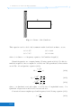
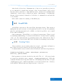
4.7
HM Panel
When all these necessities are put together, it leads to creating a sample of
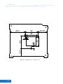
a panel with the cantilever. The panel is called HM panel. Final version is in the
picture Fig. 4.5. In the drawing position of the coil is shown and there is a permalloy
under it. Dimensions of the cantilever are 13 mm × 67 mm × 1 mm.
Additional parameters of carbon-fibre composite are Young’s modulus which is
𝐸 = 34 GPa and material density 𝜌 = 1700 kg · m−3 .
4.8
Measured Parameters
One of the most important parameters of the material is Young’s modulus.
Additional parameter is an attenuation of oscillations during measurement.
16/75
4.8 Measured Parameters
012345678
0197
9
197
9
012337
9
Fig. 4.5: Drawings of HM panel
4.8.1
Young’s Modulus of Elasticity
Young’s modulus is synonym for elastic modulus. It measures stiffness of an
elastic material to characterize materials. Modulus is characterized as ratio of stress
to strain and used for calculation of natural frequencies of the cantilever [11]. The
issue about natural frequencies is described in detail in the thesis of my colleague
Martin Urban [1].
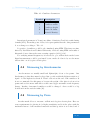
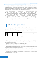
4.8.2
Attenuation of Signal
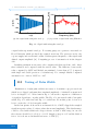
Measuring attenuation of the signal is made for verification of elasticity of material. This parameter is only additional to natural frequencies. In the picture Fig. 4.6
is sample of signal which has been measured on the HM panel. It produced damped
oscillations with almost exponential envelope.
There are several ways how to get exponential envelope. One is the electrical
way that rectifies the signal and filters it with low pass filter. There is one disadvantage though – because of the low amplitude only single diode rectifier can be used.
Another option for this purpose is to design a rectifier made of operation amplifiers.
This way has been rejected because of higher consumption of energy and it is not
necessary to implement it in a physical way.
17/75
4. Mechanical Changes Measurement
400
300
200
U [mV]
100
0
-100
-200
-300
-400
0
0.1
0.2
0.3
0.4
0.5
0.6
0.7
0.8
0.9
1
t [s]
Fig. 4.6: Sample of signal
4.9
Computing Process of FFT
Fast Fourier Transform is based on Discrete Fourier Transform (DFT) – equation
(4.14), but it is quicker and more suitable for calculation on Personal computer (PC),
Microcontroller (MCU), etc. How to get FFT from DFT is more described in the
Martin Urban’s thesis [1]. Here is only one of the possibilities of implementing it to
the Microcontroller.
𝑌k =
−1
2𝜋𝑟𝑘
1 𝑁∑︁
𝑦𝑟 𝑒−𝑗 𝑁
𝑁 𝑟=0
(4.14)
Fast Fourier Transform has two phases, one is bit reversing and second is the
main computing process. Bit reversing is shown in the Tab. 4.2 where address of a
point is swapped with the other. This operation can be solved in the same memory
space as original signal.
18/75
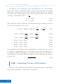
4.9 Computing Process of FFT
Tab. 4.2: Bit reversing
𝑥0
𝑥1
𝑥2
𝑥3
𝑥4
𝑥5
𝑥6
𝑥7
. . . 000
. . . 001
. . . 010
. . . 011
. . . 100
. . . 101
. . . 110
. . . 111
000
100
010
110
001
101
011
111
. . . 𝑥0
. . . 𝑥4
. . . 𝑥2
. . . 𝑥6
. . . 𝑥1
. . . 𝑥5
. . . 𝑥3
. . . 𝑥7
FFT process is sums of points (x) as show in picture Fig. 4.7 (based on CooleyTukey method Radix 2) and detail of one butterfly is in the following picture Fig. 4.8.
Fig. 4.7: Flowchart of computing FFT with N=16 points
k
A
B
An = A+BW
k
t
W
-1
Bn = A-BWk
Fig. 4.8: Detail of a butterfly
19/75
4. Mechanical Changes Measurement
The FFT process is divided into stages, their number is log 𝑁 . The flowchart
Fig. 4.7 has 4 stages of butterflies, where on the left side is the bit reversed input
signal and on the right side is the final spectrum. Each butterfly is computed
according to Fig. 4.8 using equations (4.15, 4.16). Complex points A and B represent
2𝜋𝑘
each stage of butterflies and 𝑊 𝑘 = 𝑒−𝑗 𝑇 .
𝐴𝑛 = 𝐴 + 𝐵𝑊 𝑘
(4.15)
𝐵𝑛 = 𝐴 − 𝐵𝑊 𝑘
(4.16)
These equations could be divided into real and imaginary part of numbers as shown
in six following equations (4.18 - 4.23)
2𝜋𝑘
2𝜋𝑘
𝐶 = 𝐵𝑊 = [ℜ (𝐵) + 𝑗ℑ (𝐵)] · cos
− 𝑗 sin
𝑇
𝑇
(︃
)︃
𝑘
(4.17)
⇓
2𝜋𝑘
2𝜋𝑘
ℜ (𝐶) = ℑ (𝐵) sin
+ ℜ (𝐵) cos
𝑇
𝑇
(︃
)︃
(︃
)︃
2𝜋𝑘
2𝜋𝑘
ℑ (𝐶) = ℑ (𝐵) cos
− ℜ (𝐵) sin
𝑇
𝑇
(︃
)︃
(︃
)︃
(4.18)
(4.19)
ℜ (𝐴𝑛 ) = ℜ (𝐴) + ℜ (𝐶)
(4.20)
ℑ (𝐴𝑛 ) = ℑ (𝐴) + ℑ (𝐶)
(4.21)
ℜ (𝐵𝑛 ) = ℜ (𝐴) − ℜ (𝐶)
(4.22)
ℑ (𝐵𝑛 ) = ℑ (𝐴) − ℑ (𝐶)
(4.23)
One butterfly has six additions and four multiplication operations. It is not so hard
to calculate on small MCUs in case that values of sine and cosine functions are
precalculated. When all butterflies are computed, the last step is to get values of
every frequency of the signal. This is performed in absolute value as in the equation
(4.24) [12–14].
√︁
|𝑥| = ℜ(𝑥)2 + ℑ(𝑥)2
(4.24)
4.10
Computing Process of Attenuation
Envelope of the signal represents attenuation. By using signal processing damping constant, Attenuation of system (𝛿) is extrapolated.
20/75
4.10 Computing Process of Attenuation
The process consists of a few steps:
1.
2.
3.
4.
Rectify signal
Compute moving averages
Logarithm signal
Compute least square method
4.10.1
Rectify and Moving Averages
Signal rectification is quite simple task. It is only makes an absolute value
over the sampled signal. When it is performed, the next step is to compute moving
averages, which is only sum of points in time divided by number of point. Expression
for moving averages is in equation (4.25).
𝑥𝑖 =
𝑘+𝑖
1 ∑︁
|𝑥𝑛 |
𝑘 𝑛=𝑖
𝑖 ∈ Z,
𝑖 ∈ ⟨0; 𝑁 − 𝑘)
(4.25)
Where 𝑥 is Point of signal, 𝑁 is Number points of signal, 𝑘 is Number points of
moving averages.
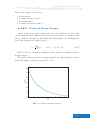
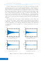
The result of this step is in the following chart Fig. 4.9. Signal length is 𝑁 =4096
points and number of moving averages is 𝑘 = 512.
120
100
A (mV)
80
60
40
20
0
0
0.1
0.2
0.3
0.4
0.5
0.6
0.7
0.8
t (s)
Fig. 4.9: Result of moving averages
21/75
4. Mechanical Changes Measurement
4.10.2
Logarithm Moving Averages
Attenuation of damped oscillation is in ideal state exponential. We will suppose
that for real measured signal. Expression of any damped oscillated signal could be
this (4.26), with one modulated frequency. Simulated signal by Matlab in Fig. 4.2
has similar waveform to real measured signal Fig. 4.6, but real signal has more then
one frequency and this is only parable to this situation.
𝑦 = 𝐴 sin(𝜔𝑡)𝑒−𝑡𝑏
(4.26)
Using moving averages to the simulated damped signal gets something similar
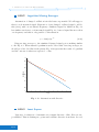
to the Fig. 4.9. When natural logarithm is used to the result of moving averages, we
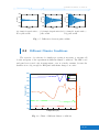
should get a line. Red line in the picture Fig. 4.10 represents the result of logarithm
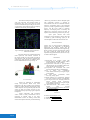
and the outcome is what was expected – a line.
5
4.5
4
3.5
A (dB-ln)
3
2.5
2
1.5
1
0.5
0
0
0.1
0.2
0.3
0.4
0.5
0.6
0.7
0.8
0.9
1
t (s)
Fig. 4.10: Attenuation with directive
4.10.3
Least Square
Last step of evaluation of attenuation is compute directive of line. Here are two
possibilities. First is defining two points and calculate directive from them. Second,
22/75
4.10 Computing Process of Attenuation
more sophisticated and more computing expensive is using an approximation of
curve, but more precise than using method of two points.
The most elementary is linear approximation called least square method or linear
regression. Also waveform could be better approximated by a higher degree of
regression or another type such as exponential or logarithm.
For our purpose linear regression is enough and its representation is equation of
line, for example as 𝑦 = 𝑘𝑥 + 𝑞, where Offset of line (𝑘) is computed by equation
(4.27) and Offset of line (𝑞) is computed by (4.28).
𝑘=
𝑞=
𝑁
∑︀𝑁
𝑖=1
∑︀𝑁
𝑖=1
𝑥𝑖 𝑦𝑖 −
𝑁
∑︀𝑁
𝑥2𝑖
∑︀𝑁
𝑁
∑︀𝑁
∑︀𝑁
𝑖=1
2
𝑖=1 𝑥𝑖 −
𝑖=1
𝑦𝑖 −
[︁∑︀
𝑁
𝑖=1
∑︀𝑁
2
𝑖=1 𝑥𝑖 −
𝑥𝑖
𝑖=1
[︁∑︀
∑︀𝑁
𝑥𝑖
𝑥𝑖
𝑁
𝑖=1
𝑖=1
]︁2
∑︀𝑁
𝑥𝑖
𝑦𝑖
(4.27)
𝑥𝑖 𝑦𝑖
(4.28)
𝑖=1
]︁2
where 𝑁 is Number of point least square method, 𝑥i Time point in least square
method, 𝑦i Amplitude point in least square method, 𝑘 Directive of line, 𝑞 Offset of
line,
Linear regression could be used for the whole signal – only in the case that signal
is a line in the whole length. Although, this claim is questionable. For safer and
more reliable result, in autonomous mode, it is recommended to use small part of
the signal. The best part is the beginning. In the picture Fig. 4.10 is a result of
least square. The blue line is an outcome directive of linear part of signal. The
approximation is used in length approx. 0.2 s. Length of least square method is
configurable for further improvement of measurement on orbit, in depends on quality
of sampled signal.
23/75
5
Device for Mechanical
Measurement
Changes
The idea of measuring mechanical changes is to measure resonance frequency of
the material and recursively calculate elastic modulus and other properties. So it
leads to creation of the measurement system – HM panel and HM board.
5.1
HM panel
Fig. 5.1: Picture of HM panel
Health Monitoring panel is made from carbon-fibre material and milled cantilever
shown on the drawing Fig. 4.5. HM panel is mounted as tilting panel on the top of
the satellite, as shown on Fig. 3.1a.
The HM panel consists of some important parts for measuring, like excitation
coil which attract permaloy target glued on the cantilever, under the coil. It causes
25/75
5. Device for Mechanical Changes Measurement
oscillations which are measured by piezo-electric element glued on the most stressed
position at the opposite side of the cantilever. Piezo is situated in place of the
highest mechanical changes. Assembled HM panel is in the picture Fig. 5.1.
Surface of the panel is covered by two reflective materials. There is nickel compound on the left side and golden compound on the right side. These materials
should reflect thermal radiation for example from the Sun.
Health Monitoring panel has six sensors PT1000 which measure temperature
transmission through the panel. Temperature is also important factor for calibration
of measurement, because properties of carbon fibre material could change. Final
assembling of these sensors are shown in the pictures Fig. 5.2.
(a) Front side
(b) Back side
Fig. 5.2: Detail of HM panel
All temperature sensors are connected to the measure board which measure temperature from almost all PT1000. Board could be called by any payload through
I2 C interface via CSP. Wires from coil and piezo are connected to the HM board
which processes all measurements of mechanical changes. Piezo is connected to the
connector marked as Piezo and coil is connected to the connector called Coil.
26/75
5.2 HM board
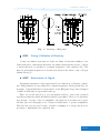
5.2
HM board
Health Monitoring board is shown in the picture Fig. 5.3 which consists of
parts such as main connector which is not standardized for CubeSat, because of the
weight and also board is the last one in row in the probe. So it is not necessary to
connect all signals to the board, only power supply and I2 C interface. Next part is
external oscillator connected to the MCU ATxMega128A4U from Atmel company.
Microcontroller is responsible for signal sampling from piezo and excitation of coil
assembled on HM panel.
Oscillator
Power
switch
Piezo
connection
Thermometer
MCU
SRAM
Fig. 5.3: Picture of HM board with highlighted parts
5.2.1
Microcontroller for Payloads
Microcontroller ATxMega128A4U has been chosen for payloads, which is one of
many compatible devices with CSP. It is quite powerful MCU for simple tasks, such
as signal sampling, temperature measurement, communication with other boards,
etc. Basically it is focused on easy tasks but for measuring mechanical changes it is
necessary to get the frequency.
One of the possibilities how to find out the frequencies is to calculate period.
Using this method is not too much reliable for more then one frequency contained
in sampled signal. So it have to calculate FFT. It is not too much suitable for this
27/75
5. Device for Mechanical Changes Measurement
purpose, because of the computing power, but with more time for calculating, it is
possible to do it. The best way to process FFT is use a DSP Microcontroller. It
will calculate it in shorter time, because it has specialized instructions for it.
The MCU ATxMega128A4U is from AVR family of chips and value 128 signifies
the size of internal Flash memory, it has 128 kB of it. Some selected parameters of
the Microcontroller are in the table Tab. 5.1.
Tab. 5.1: Parameters of MCU ATxMega128A4U [15]
Type
Parameters
Description
Flash
SRAM
EEPROM
Speed
128 kB
8 kB
2 kB
up to 32 MHz
Size of internal program memory
Size of internal data memory
Size of internal data memory, non-volatile
Maximal speed of external/internal oscillator,
crystal, . . .
Number of single ended inputs
Number of differential inputs
Resolution of ADC
Number of 16-bits Timers/Counters in MCU
Tolerance of supply voltage in range of frequencies 0 − 32 MHz
ADC
ADC
ADC
Timers/Counters
Supply
5.2.2
up to 12
up to 8
12 bits
5
2.7 − 3.6 V
Oscillator
The source of accurate clocks is necessary for signal sampling. It means finding
the best crystal or oscillator for this purpose. Common crystals have low temperature stability, about ± 25 ppm in −30 ℃ to + 80 ℃ temperature range.
The oscillator TCX0-1A is very precise and is tuned to 16.470 MHz. Frequency
stability vs. temperature is better then ± 2 ppm. Oscillator usually comes with
an internal capacitive trimmer, but for space mission it would be very unsuitable
because it could change frequency during the mission and the results would be
invalidated. Evaluation depends mostly on frequency change of cantilever in time.
That capacitive trimmer was replaced by solid capacitor with fixed value. This was
special requirement for an oscillator [16].
28/75
5.2 HM board
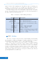
External Memory
For high number of points of FFT is necessary to have more memory space.
Internal RAM has only 8 kB and almost 3/4 of is used for variables and FreeRTOS. Because of that external memory connected to the MCU is necessary. FRAM
memory is valuable for use in space because it is more reliable then EEPROM and
SRAM. But it is quite difficult to find a suitable chip. All commonly have parallel
+3.3V
interface, so it is necessary to have many Input/Output (I/O) pins for connection
to the memory. EEPROM has one disadvantage and that erase and write cycle
takes a lot of time, about 5 ms. So+3.3V
it led to a choice of SRAM memory. It has al+3.3V
IC2
IC4is disconnected data are
most instant
write and
read cycle but when power supply
1
8
/CS VCC
CS
lost. For
required
results
are2 stored in
2 computing
7 FFT data loss does not matter, 17
SO VBAT
EP
SDA
MISO
10
1
CT
SCL
9
data-keeper. SCK 6
INT
SCK
4
5
12 Serial
As external
memory
has
Peripheral4 Interface
VSS
VDD
SI
MOSI been chosen 1 Mb of SRAM
A1
11
3
23LCV1024
GND
A0
(SPI) memory 23LCV1024 [17].
4k7
C5
100n
C11
100n
C12
100u/10V
R19
4k7
I2C thermometer
Memory
I/O
R20
5.2.3
3V
+5V
3V
+5V
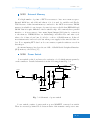
5.2.4
D
GND
Power Switch
GND
GND
ADT7420UCPZ-R2
GND
L
SDA
Power switch on the board serves for excitation of coil, which attracts permaloy
on the cantilever. Detailed schematic is in the following picture Fig. 5.4.
Switch
COIL+
53261-04
X1-1
D2
Coil
MURD620CTG COIL-
C2
2
5
6
R17
100k
R18
+
C1
+5V
2ND_SWITCH
1m5/6,3V
1k
+
R5
1m5/6,3V
BAT754A D1
+3.3V
10k
+3.3V
X1-4
SI3442CDV
T1
Q1
BSS123
GND GND
PIEZO_ON
GND
GND
Fig. 5.4: Schematic of power switch
connection
Test points
Power switch consists of parts such as power MOSFET connected as switch.
TP1
TP6
There is a reversed polarized diode between drain
of the+5Vtransistor and
powerGND
source
R7
PIEZO+
TP2
+3.3V
TP7
2ND_SWITCH
TP4
COIL+
TP9
AVCC
V_PIEZO
100k
R8
1M
R1
10k
29/75
SDA_ADT
SCL_ADT
5. Device for Mechanical Changes Measurement
for catching peaks of voltage from the coil. If the diode would be omitted it could
cause damage the transistor in the best case. In the worst case, it could destroy
whole satellite. So it is necessary. The second switch is used for separation of 5 V
and 3.3 V power supply. 5 V to the gate of transistor is more suitable for high current
through power transistor T1.
Energy for high power peak is stored in two tantalum capacitors with total capacitance of approx. 3 mF. It is enough for excitation of the coil with high amplitude
on the piezo. Amount of energy can be controlled by width of pulse to the Piezo_on.
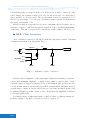
5.2.5
Piezo Connection
Piezo element is connected to the MCU’s ADC through resistor divider. Schematic
of input measurement is in the picture Fig. 5.5.
X2-2
R7
PIEZO+
V_PIEZO
10k
Piezo
100k
R8
X2-4
Shielding
1M
R1
X2-3
X2-1
53261-04
AGND
AGND
Fig. 5.5: Schematic of piezo connection
Divider reduces amplitude of the input signal. Signal is alternating around zero
voltage and minimum amplitude of input voltage must be greater then −0.4 V,
otherwise signal is clipped by internal diode. Unfortunately this problem was discovered in time when board was already created and assembled, and there was not
enough time to change it. In the end it was not a problem, measured signal could
be trimmed slightly by width of pulse to the coil and then the amplitude is reduced
to the appropriate value.
For further using of differential input of ADC is better to shift up virtual zero
(negative input) to the half of reference voltage, to approx. 1 V.
30/75
5.2 HM board
5.2.6
Thermometer
Health Monitoring board is equipped with one thermometer ADT7420 communicating through I2 C interface. Its resolution is 16 bits with sign. In the following
table Tab. 5.2 are shown other basic features.
Maximum allowed number of these devices is four, because this chip provides four
different addresses. Address can be changed by two pins A0, A1 on the package.
Rest is set by the manufacturer and the address range (in hexadecimal format) is
from 0x48 to 0x4B. Pins A0, A1 on HM board are connected to the ground –
logical zero, thermometer ADT7420 has address 0x48.
Tab. 5.2: Parameters of thermometer ADT7420 [18]
Parameter
Resolution
Temperature range
Precision
Supply
Value
up to 16 bits
−20 to +105 ℃
±0.25 ℃
2.7 to 5.5 V
Description
Maximal resolution of thermometer
Temperature range of thermometer
Accuracy of thermometer in temperature
range from −20 to +105 ℃
Power supply voltage range
Thermometer is connected through I2 C interface and the bus required external
pull-up resistors with resistance about 4.7 kΩ.
Value from the thermometer can be get by one CSP packet if any board needs
to know it. Parameters of the communication are specified in chapter 6.4.4. Delay
between command and return value is approx. 250 ms. This time is derived from the
length of conversion which is about 240 ms. All parameters are from datasheet [18].
31/75
6
Communication with Other Boards
Communication is one of the most important things. Without it, data cannot
be transmitted and boards do not know what to do. In this case, board communicates with the rest of the probe (connected to the same bus) via I2 C interface. All
boards have specific communication protocol called CubeSat Space Protocol. It is
an universal protocol specially for CubeSats.
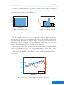
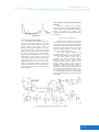
6.1
I2C Interface
Generally I2 C interface is connected via two wires SDA and SCL with common
ground. The bus required two pull-up resistors, usually in range of 470 – 10 kΩ. It
depends on specification from the manufacturer. With more devices on the bus, it
is recommended to reduce the resistance. When bus is idle, positive voltages are on
SDA and SCL wires. Visualization of the connection is on the follow figure Fig. 6.1.
Resistors RPU are not necessary at every device, one on each wire is enough.
Fig. 6.1: Schematic of connection I2 C devices [19]
Communication protocol between master and slave unit is shown on the next
figure Fig. 6.2. Communications starts with start condition – SDA falling edge
prevents SCL falling edge. Then follows 7-bits address and last bit is read (high)
33/75
6. Communication with Other Boards
or write (low). Each byte is ended by ACK. After address could follow data byte/s
from master/slave – it depends on read/write bit. When transmission is ending,
master sends NACK bit and then stop condition follows – SCL rising edge prevents
SDA rising edge. Data can change only when SCL is low [19, 20].
Fig. 6.2: Chart with communication via I2 C [19]
6.2
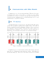
CubeSat Space Protocol
CubeSat space protocol is unified for small nanosatellites such as are in mission
QB50. The protocol is similar to TCP/IP protocol with simplified header. Header
has 32 bits and contains following parts, image representing it is in Fig. 6.3.
31 30 29 28 27 26 25 24 23 22 21 20 19 18 17 16 15 14 13 12 11 10 9
Prio
rity
Source
Destination
Destination Port
8
Source Port
7
6
5
4
3
2
F
R
Reserved
A
G
H
M
A
C
X
T R C
E D R
A P C
1
0
Fig. 6.3: CSP header
Priority is when master has more then one packet to send, packet with higher
priority will be send sooner.
Source is address of master from whom packet came.
Destination is address where the message will be sent to.
Destination Port is internal port of slave. After receiving a packet the board
performes a specific task assigned to that port.
Source Port is internal port of master. It is commonly used for ACK or returns
data to the master from slave.
Last five bits are configurations of transmission and all devices on the bus must
have same settings of these bits.
34/75
6.3 FreeRTOS
After header follows data. Maximum size of data is not generally set, but it is
not recommended to transfer huge amount of data, because transfer could overload
bus and other boards have to wait until bus is free. It has been established that
optimal size of data is up to 64 Bytes per packet. Disadvantage of sending huge
amount of data is memory demands on both sides of communication and busy line
of one transfer.
Whole CSP is suited for running on FreeRTOS [21].
6.3
FreeRTOS
FreeRTOS is shortcut for Free Real Time Operating System. This system is
multi-platform and it can run on 32-bit platform as well as on 8-bit. It is primarily
suited for embedded systems based on ARM cores but it is possible to use on small
devices such as ATxMega.
Only requirement of FreeRTOS is one dedicated system timer. Timer is used
for switching (multitasking) of each used task which are declared in the beginning
of the code. Recommended time for switching tasks is 1 ms. When shorter time is
used, it has been observed that MCU has been halted by switching between tasks.
6.3.1
Creating Tasks
Every task has some necessities when it is created – task name and function,
place where it is created, memory allocation size, task priority, . . .
Command which creates a task is called xTaskCreate and it has six parameters:
xTaskCreate(pvTaskCode, pcName, usStackDepth, pvParameters,
uxPriority, pxCreatedTask)
Each parameter is shortly described in the table Tab. 6.1 . All created tasks
are started by scheduler’s start command – vTaskStartScheduler(). With this
command all tasks start doing their functions. All running tasks has their own part
of RAM memory space, which in sum must be lower then dedicated size of memory
for FreeRTOS. This prevents any dangerous state or data loss.
35/75
6. Communication with Other Boards
Tab. 6.1: xTaskCreate Command Parameters [22]
Parameter
Description
pvTaskCode
pcName
usStackDepth
pvParameters
uxPriority
pxCreatedTask
Function pointer
Task name
Stack size
Parameters of the task
Task priority
Used for backward handle
Every task usually works in infinite loop similar to main function. The next
Code 6.1 represents example of a task without any function – only body [22].
Code 6.1: Main loop of any task
int task_name(void * pvParameters){
// initialization here
while(1){
// do something here
}
return 0;
}
6.4
Communication with HM Board
I would like to express big thanks to my colleague ing. Tomáš Báča for help
with the basics of implementing FreeRTOS and CSP to the HM board.
As is written previously, all boards communicate via CSP and the HM board has
several commands coupled with ports and its address is 6. Between basics functions
of all board are ping that board is still alive and House keeping (HK) data – it
returns information about board. Between user defined commands are for example
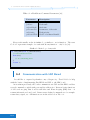
return data, signal, etc. All functions are in the table below Tab. 6.2.
36/75
6.4 Communication with HM Board
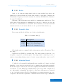
Tab. 6.2: Communication ports of HM board
Port number
18
19
20
21
Description
Measure starts
Returns signal to DK
Returns results of measurement
Returns temperature of HM board
Meaning of commands from table Tab. 6.2 are as follows:
6.4.1
Measure Starts
Measuring starts only when HM board gets packet to the port number 18.
Packet could be empty or contain anything, but it does not matter to the program
what came. Response to the originator is simple – ackMes as text. When signal is
sampled, all that is calculated returns results to the DK.
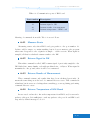
6.4.2
Returns Signal to DK
When this command is called, MCU returns signal of previously sampled to the
DK divided into many chunks, each with predefined size – 32 Bytes. When signal is
transmitted to the ground, there it will be reconstructed.
6.4.3
Returns Results of Measurement
This command returns only results that have been calculated previously. It
means the same thing as at the end of command Measure starts. This command is
redundant, but it serves as a backup when something goes wrong during performing
command Measure starts.
6.4.4
Returns Temperature of HM Board
In case any board needs to know the temperature from HM board, it can send a
packet to this port. It is sufficient to send any packet to the port 21 and HM board
responds by defined message Code 6.2:
37/75
6. Communication with Other Boards
Code 6.2: Respond to Get Temperature Command
typedef struct __attribute__ ((packed)){
uint16_t temperature;
// temperature from ADT7420
}hm_temperature_t;
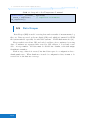
6.5
Data Keeper
Data Keeper (DK) is used for storing data such as results of measurements, log
files, etc. Data are saved on Secure digital (SD) card, which is formatted by UFFS
file system suitable especially for embedded systems – NAND flash memories [23].
Every result is stored into DK and each board has a few containers for storing
data. Containers are separated files sorted by CSP address of board and a variable – storage number. All data must be divided into chunks, each with unique
identification number.
Each storage, when it is created, has fixed data space for configuration data –
chunk number zero. When chunk zero is used for configuration data, it must to be
created before the first use a storage.
38/75
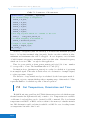
7
Measurement Process in HM board
Before the measurement starts, it is necessary to send activation sequence to the
board. It is provided by OBC through CSP command. Header of CSP contains
destination port which correspond to specific command. Port chosen for the main
measurement is 18 as written in the Tab. 6.2.
Process of the main measurement is divided into several steps:
1.
2.
3.
4.
5.
6.
7.
8.
9.
Read parameters of measurement from DK
Get temperatures from all sensors – from Measure Board
Get orientation of the probe
Get actual board time
Excitation of coil for a defined time (loaded from DK)
Sampling of signal
Signal processing – FFT
Signal processing – attenuation
Store data to the DK
7.1
Read Parameters of Measurement
Parameters of measurement are stored in DK, storage number 1. Configuration
contains mainly parameters around computing Young’s Modulus of Elasticity, such
as range of frequencies where natural frequency is looked for, decimation frequency,
pulse length to the coil and number of points of least square method from the
beginning of signal. Whole structure of configuration is in listing Code 7.1.
39/75
7. Measurement Process in HM board
Code 7.1: Parameters of Measurement
typedef struct __attribute__ ((packed)){
// 3x tolerance range of frequencies
uint16_t f1_min;
uint16_t f1_max;
uint16_t f2_min;
uint16_t f2_max;
uint16_t f3_min;
uint16_t f3_max;
// how long is power switch on - current to the coil
uint8_t
time_power_switch_on;
// to which frequency is decimated to
uint16_t decimation_factor;
// length of least squares
uint16_t length_of_ls;
}hm_config_t;
Accuracy of frequency (first six variables) is in Hertz and minimum (fx_min)
have to be less then maximal value (fx_max). In the case this condition is false,
minimum and maximum value will be swapped. In case frequency exceeds limits
of half decimation frequency, maximum value is set this value. Maximal frequency
which can be set is 65 kHz – enough for this application.
Time for power switch on (time_power_switch_on) is in 1/10 of ms – number
15 corresponds to 1.5 ms. The maximum time is 25.5 ms (255).
Decimation factor (decimation_factor) is a value for calculation of spectrum
from sampled signal. This value is division factor for decimation of sampled signal,
to reduce spectrum of signal.
The directive of exponential envelope is calculated by the least square method.
length_of_ls is constant which specifies computing range of this method. Value
represents number of calculation points of linear regression.
7.2
Get Temperature, Orientation and Time
Health Monitoring panel has six PT1000 thermometers in total which measure
thermal transfer through material and/or surface of it. Temperatures are available
on Measure board and they can be obtained by CSP command. The board return
temperatures and MCU on HM board store them to the memory for further transfer
into DK. Orientation and board time is available on OBC. Process of reading is same
as temperature but with other board.
40/75
7.4 Signal Processing – FFT
7.3
Excite of Coil and Sampling of Signal
When all parameters are loaded and other variables are read from the boards,
measurement process can start. Microcontroller has one dedicated timer for timing
of excitation coil which stops excitation.
Also one timer is dedicated for sampling of signal with higher priority of interrupt
– for precision timing. All points are sampled and averaged four times and then
stored into SRAM to the space dedicated for sampled signal. Number of points
is 4096 at 𝑓s = 4 kHz. It covers a little bit more then 1 s of signal. From this
determination of Sampling frequency is possible to have spectrum up to 2 kHz.
7.4
Signal Processing – FFT
The most important part of signal processing (for our purpose) is computing
FFT to find out resonant frequencies of sampled signal. More detailed description
about meaning of looking for frequencies is in chapter 4.8.1. Introduction to the
FFT process is in Martin Urban’s thesis [1] and in chapter 4.9 with all equations for
calculations.
Here I will only simply describe how to calculate it in 8-bits MCU and the
implementation into the Microcontroller. The whole FFT computing process has
two parts – address bit reversing and the actual FFT process.
7.4.1
Decimation and Address Bit Reversing
Decimation is used for reducing the spectrum of signal, but Shanon-Niquist
theorem of 𝑓s ≥ 2𝑓max for searching frequency must be followed, in this case 𝑓max .
With the same length of window for computing FFT, resulting spectrum has better
resolution in frequency. Sampled signal has default 𝑓s = 4 kHz and decimation factor
is 4. It is according to new sampling frequency 1 kHz. Decimation factor could be
changed by the setting stored in DK – decimation factor. But if the factor is one,
decimation will not be used.
Bit reversing is one of the requirements for computing FFT when is used Decimation in time (DiT) or Decimation in frequency (DiF) method. Main difference
between DiF and DiT is in order of performing bit reversing and FFT process. Decimation in time consists of this: bit reversing and then FFT process and Decimation
41/75
7. Measurement Process in HM board
in frequency has reversed order.
Process of bit reversing is simple. Take one point of signal with known address,
swap all address bits and store the point into this changed address. In the table
Tab. 4.2 is visualised this claim, addresses for example are in binary form in length
of 3 bits.
From this point of view it is recommended to use DiT method and combine
advantageous decimation with bit reversing. Every point is loaded and stored one
time from/into the memory. For simplification of reversing, all bit reversed addresses
are stored in array in Flash memory of MCU. In the following code listing Code 7.2
is implementation of decimation and bit reversing.
Code 7.2: Decimation and bit reversing
void decimate_and_store(void){
// here is variables and verification
// of decimation frequency in configuration
// storing and bitreversing raw signal into spi memory
for (u_int16 i=0; i<NO_POINTS; ++i) {
position = pgm_read_dword_far(&bitrev[i]);
decimation_position = (long) position * DECIMATION_FACTOR;
if (decimation_position<MEM_SIGNAL_POINTS) {
read_data = spi_mem_read_word(decimation_position*2 +
MEM_SIGNAL_BEGIN) - signal_offset;
point.real = read_data;
}
else
point.real = 0;
// store into SPI memory
spi_mem_write_complex((long) MEM_FFT_BEGIN + i*8, point);
}
}
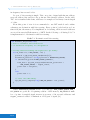
Where DECIMATION_FACTOR is ratio of 𝑓s and 𝑓dec , MEM_SIGNAL_BEGIN, MEM_FFT_BEGIN are positions of beginning address of SPI memory, NO_POINTS is number of points of sampled signal, bitrev is an array of bit reversed addresses and
signal_offset is value for elimination of DC part of signal [12].
42/75
7.4 Signal Processing – Attenuation
7.4.2
FFT Process
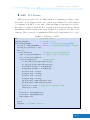
FFT process is based on Cooley-Tukey method of computing according to equations (4.18 - 4.23). Functions sine and cosine are precalculated in a table instead
of computing it in MCU to save time. Final spectrum is represented as an absolute value of complex point (4.24). For our purpose it is necessary to know only the
maximum peak and from this point of view is square root omitted to save time of calculations. The code used for computing the FFT is in following listing Code 7.3 [13].
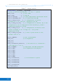
Code 7.3: Calculation of FFT
n=1;
// actual state
angf=NO_POINTS/2;
// twiddle factor
while(n<NO_POINTS){
// number of iterations log2(NO_POINTS)
pointer_A = MEM_FFT_BEGIN; // address of beginnig memory space for FFT
pointer_B = pointer_A + n*8;
Fnk = 0;
for(k=0;k<n;k++){
// distance between butterflies
dsin = read_sincos(Fnk++); // read sin and cos from table
dcos = read_sincos(Fnk++);
for(s=0;s<angf;s++){
// butterflies
A = spi_mem_read_complex(pointer_A);
B = spi_mem_read_complex(pointer_B);
C.real=(B.real*dcos - B.imag*dsin);
C.imag=(B.real*dsin + B.imag*dcos);
B.real=A.real - C.real;
B.imag=A.imag - C.imag;
A.real=A.real + C.real;
A.imag=A.imag + C.imag;
spi_mem_write_complex(pointer_A,A);
spi_mem_write_complex(pointer_B,B);
pointer_A += n*16; // nextpoint in memory 2x 2x4B
pointer_B += n*16;
}
pointer_A-= (NO_POINTS-1)*8;
pointer_B-= (NO_POINTS-1)*8;
Fnk+=(angf-1)*2;
}
n<<=1;
angf>>=1; // twiddle factor /2
}
43/75
7. Measurement Process in HM board
7.5
Signal Processing – Attenuation
After computing FFT, the next step is to calculate attenuation of signal, which
is expected to has exponential envelope. By using equation (4.27) the directive
is computed – attenuation of signal, from linearised signal. There is a dedicated
memory space for the whole computing process of directive and has same size as
sampled signal. Sample of code is in the listing Code 7.4 where is only the main
part of calculation.
Code 7.4: Calculation of attenuation
copy_signal_attenuation(); // copy and decimate signal
average_signal();
// rectify, average and logarithm the signal
for (i=OFFSET_AVERAGING_POINTS; i<((int)OFFSET_AVERAGING_POINTS + n);
i++){
loaded_value = spi_mem_read_word(i*2 + MEM_ATTENUATION_BEGIN);
point = (float) loaded_value;
sum_x_i_y_i *= point;
sum_x_i += i;
sum_y_i += loaded_value;
sum_x_i_squared += i * i;
}
// recalculation from samples to the time
sum_x_i_y_i /= fs;
sum_x_i /= fs;
sum_x_i_squared /= (fs * fs);
reg_k = (n*sum_x_i_y_i - sum_x_i*sum_y_i) / (n*sum_x_i_squared sum_x_i*sum_x_i)*100;
reg_q = (sum_x_i_squared*sum_y_i - sum_x_i*sum_x_i_y_i) /
(n*sum_x_i_squared - sum_x_i*sum_x_i);
where OFFSET_AVERAGING_POINTS is constant offset in time (samples) since least
square is computed, MEM_ATTENUATION_BEGIN is offset in memory where stored signal for computing attenuation begins, n is number of averaged points.
The function copy_signal_attenuation() is only copying signal from one part
of external memory to the other and decimate the signal according to DECIMATION_FACTOR.
44/75
7.7 Conclusion
The function average_signal() consists of the following processes, rectifying of
signal using abs function (make absolute value), moving average for curve smoothing
and logarithm them for linearisation of signal according to chapter 4.10.1 and 4.10.2.
Code has one main for cycle where all sums in this loop according to equation
(4.27).The for cycle does not calculate with time, because it would mean additional
time for calculation. Recalculation to the time is performed after the for loop using
reciprocal value of 𝑓s .
Final results of least square method are in reg_k which is a directive of line –
our attenuation and in reg_q is an offset of line. Only directive is stored, offset is
not stored because it does not corresponds to the maximal value of original signal
and also it is not necessary for further evaluation.
7.6
Store Results
All measured and received data will be saved to the DK with the following
structure Code 7.5 and than transmitted to the earth for next process.
7.7
Conclusion
The small MCU ATxMEGA128A4U is able to compute FFT with 8192 points,
but it takes a lot of time, approx. 15 s because the code is not very optimized for
speed. On orbit there will be a lot of time for this task – it is established that the
shortest delay between measurements will be at least 5 min. So 15 s is enough with
a huge reserve – it is not calculated with other delays from getting the temperature,
time from OBC and orientation of the probe. Totally, it is estimated on around 2030 s from start command to saving the results. When is required also raw signal, to
this time is added approx. next 15 s to store the data.
45/75
7. Measurement Process in HM board
Code 7.5: Output structure
typedef struct __attribute__ ((packed)){
// status of HM board and HM panel - 0 = OK, 1 = problem
uint8_t xtal
: 1; // xtal works
uint8_t sram
: 1; // sram OK
uint8_t loaded_MB
: 1; // loaded temperatures from Measure Board
uint8_t loaded_OBC_time : 1; // loaded time from OBC
uint8_t config_out_dec : 1; // configuration is invalid,
// decimation = 0 or > 4000 Hz - applicated 1000 Hz
uint8_t config_out_freq : 1; // configuration is invalid, any of the
// frequencies is out of range greater then decimate_to_f Hz/2 // applicated decimate_to_f/2 Hz
uint8_t config_out_ls
: 1; // configuration is invalid, least
// square averaging is out of range 200 - 1000 points // applicated 200 Hz
uint8_t config_out_power : 1; // time of power switch is zero,
// default value is 10
uint32_t OBCTime;
// time of measurement
int16_t f1;
// 3x frequencies
int16_t f2;
int16_t f3;
int16_t attenuation_directive; // (k) directive of attenuation // from equation y = kx + q
int16_t tempADT;
// temperature from ADT thermometer
int16_t temp1;
// 6x temperature from HM panel
int16_t temp2;
int16_t temp3;
int16_t temp4;
int16_t temp5;
int16_t temp6;
int16_t orientation1;
// 5x orientation of probe
int16_t orientation2;
int16_t orientation3;
int16_t orientation4;
int16_t orientation5;
} hm_output_data_t;
46/75
8
Measurements, Testing and Results
100
100
Magnitude 20 log10|Y(k)|
Magnitude 20 log10|Y(k)|
It is necessary to verify the final device in many climate conditions such as
temperature changes, pressure, etc. same as reproducibility of measurement in the
same conditions. All measurements precede theoretical calculations and simulations
of gained signal, natural frequencies of cantilever, etc. and then we compare real
data to theoretical results.
At first it is good to know natural frequencies of oscillated cantilever. From
equation (4.11) natural frequencies are gained. For HM panel with these parameters:
• cantilever dimensions 13.2 × 67.4 × 1.2 mm
• elastic modulus is 𝐸 = 3.8 · 1010 Pa
• material density is 𝜌 = 2300 kg · m−3
the first three natural frequencies are 171.6 Hz, 1075 Hz, 3011 Hz. The first two
frequencies satisfy Shanon-Niquist theorem that says the sampling frequency (𝑓𝑠 =
4 kHz) must be at least two times higher then maximum sensed frequency. Third
and next cannot be directly measured.
80
60
40
20
0
0
500
1000
1500
2000
Frequency (Hz)
(a) Spectrum of panel mounted in clamp
80
60
40
20
0
0
500
1000
1500
2000
Frequency (Hz)
(b) HM panel mounted on a frame and all
hanged on wire
Fig. 8.1: Difference in spectra with different placement
Pictures of real measured signal in Fig. 8.1 are comparing the difference of spectrum in dependence on placement of HM panel. Both charts contain first two natural frequencies, but the second one Fig. 8.1b has extra peaks on frequencies around
300 Hz and 750 Hz. Peaks are probably caused by other resonances of a metal frame,
47/75
8. Measurements, Testing and Results
because the left chart does not have them. Health Monitoring panel mounted in jaws
at the fixed side of cantilever and it may be considered a reference sample for further
evaluation.
Spectrum above Sampling frequency (𝑓s )/2 does not affect main part of it, only
smooths it a little. This statement is based on using Finite impulse response (FIR)
filter on sampled signal, where differences in spectrum with and without using FIR
filter are minimal. Comparison of them is in the pictures Fig. 8.2.
100
Magnitude 20 log10|Y(k)|
Magnitude 20 log10|Y(k)|
100
80
60
40
20
0
0
500
1000
1500
2000
80
60
40
20
0
0
Frequency (Hz)
500
1000
1500
2000
Frequency (Hz)
(a) Spectrum of signal without using FIR (b) Spectrum of signal with using FIR filter
filter
Fig. 8.2: Differences in spectra without and with using FIR filter
8.1
Beginning of Research
The main part of research has began in the spring of 2014 when the highest
possible resolution in frequency was expected around 0.1 Hz. At the beginning of
research we took only the part to 250 Hz, where the main peak, the first natural
frequency of the cantilever is located. All these claims are based on similar spectrum
to reference Fig. 8.1a which was sensed by oscilloscope for the first time.
At first it was required to learn about the used Microcontroller ATxmega128A4u,
so we got development kits with this MCU. Picture of it is in the photo Fig. 8.3.
The kit consists of main MCU with three user buttons, alphanumeric Liquid crystal display (LCD), two LEDs and Universal synchronous and asynchronous serial
receiver and transmitter (USART) which could be used for bootloader for downloading a new version of FW into the chip.
The kit has the advantage during debugging in that display could serve feedback
what is happening in the MCU. USART can be advantageously used for downloading
measured data or uploading commands for affecting processes in the chip.
48/75
8.2 Research During Internship in Japan
Fig. 8.3: Photo of development kit [24]
One of the first things what were needed to do was commissioning ADC and
downloading signal via USART. ADC was set-up as single ended input on first analog
input of MCU with a result saving into internal SRAM. Amount of samples, which
could be saved, is estimated at 2500 points in 12 bits resolution (16 bits variables).
These points are downloaded into PC and then evaluated. For evaluation of signal
in the computer, environment Matlab was used. Next step was implementing the
FFT, based on sampled and evaluated signal.
8.2
Research During Internship in Japan
Part of the research I and my colleagues Martin Urban and Veronika Stehlíková
did, was done during summer internship in 2014 at Hosei University in Tokyo,
Japan. There has been done implementing of FFT into chip together with storing
data to the external SPI memory. Knowledge about signal processing was provided
by professor Kazuo Yana, Ph.D., to whom I would like to express huge thanks [25],
as well to other staff of the University for providing laboratories and equipment for
testing and verifying progress of implementing functions into the MCU.
First step of verification was done on sinusoidal signal with triangular envelope,
as shown in the Fig. 8.4. The implemented FFT was calculated with 256 points only
(time saving), for verifying that the algorithm works with external memory. Results
were what had been expected. More points of FFT calculation were added later, to
one of the last versions of Firmware (FW) or for the calibration measurement.
Second step was verification of signal attenuation. Basics could be performed
on triangular envelope, but to get closer to real situation, it is better to measure
49/75
1000
U (mV)
500
0
-500
-1000
0
0.5
1
1.5
Magnitude 20 log10|Y(k)|
8. Measurements, Testing and Results
100
50
0
0
t (s)
(a) Sine signal with triangular envelope
100
200
300
400
500
Frequency (Hz)
(b) Spectrum of signal with using FIR filter
Fig. 8.4: Signal with triangular envelope
a signal with exponential envelope. For testing purposes a generator was made at
Hosei University which produced the required waveform. The generator needs only
a power supply and an external oscillator with requested frequency of the signal with
defined output amplitude [26]. Computing process of attenuation is in the chapter
4.10.
Resulting attenuation was sent to the computer and then saved into a file. After
that evaluated and compared with theoretical value. The difference between the
value computed by MCU and Matlab was minimal - better than 0.5 % (compared
with single and double precision of calculations). For example Matlab computed
attenuation as −4.08 vs. MCU as −4.07.
8.3
Testing of Pulse Width
Examination of right pulse width is necessary to determine a proper waveform
which is not clipped and must have maximal amplitude of ±400 mV as mentioned
before in chapter 5.2.5. Waveforms in Fig. 8.5 shows the comparison of differences
of signal in dependence on pulse width. The Fig. 8.5a was sensed with 0.5 ms pulse
width, Fig. 8.5b with 1 ms and Fig. 8.5c with 2 ms. From this point of view it is
best to excite the coil by 1 ms pulse width.
In the last picture is shown how an internal diode of MCU clipped the sampled
signal in negative values. Positives values has normal amplitude. This disadvantage
could be solved with additional voltage reference at half of ADC range, in our case
the reference should be (3.3/1.6)/2 = 1.03 V. Supply voltage is 3.3 V and the division
factor 1.6 is chosen as an internal reference of ADC [15].
50/75
400
400
200
200
200
0
-200
-400
0
U (mV)
400
U (mV)
U (mV)
8.4 Different Climate Conditions
0
-200
0.5
1
-200
-400
0
1.5
0
0.5
t (s)
1
-400
0
1.5
0.5
1
t (s)
1.5
t (s)
(a) Sampled signal with too (b) Sampled signal with ideal (c) Sampled signal with too
short pulse width
pulse width
long pulse width
Fig. 8.5: Differences between pulse widths
8.4
Different Climate Conditions
The creation of a reference for further processing is necessary to measure all
boards and parts of the experiment in different climate conditions. The HM board
and panel were tested only in temperature oven, not in the vacuum, because the
chamber is not big enough for HM panel with frame hanged on a wire.
1000
5
f1
f2
f3
attenuation
900
800
0
Attenuation (-)
Frequency (Hz)
700
600
500
400
-5
300
200
100
20
40
60
80
100
120
140
160
-10
180
Temperature (°C)
Fig. 8.6: Chart of different climate conditions
51/75
8. Measurements, Testing and Results
We made climate testing only in heated oven. This test was performed in temperature range from 25 ℃ to 176 ℃ as shown in the chart Fig. 8.6, where frequency of
first natural frequency (f1 line) is almost unchanged in the whole range of measurement conditions. Second line (f2) is an now unspecified frequency peak at 300 Hz,
probably is natural frequency of the frame. Its changes began at temperature around
140 ℃. Third frequency (f3) should not be here, it is mirrored from 1050 Hz. This
fact is caused by undersampled signal, only 2 kHz sample rate, on testing equipment.
This test was performed at time, when we were determining sampling frequency and
method, how to get the most precise frequency (0.1 Hz resolution) of the first natural
frequency.
400
400
200
200
U (mV)
U (mV)
The frequency line f3 has began to change significantly at 100 ℃. This could
be affected by the quality of glue hardening, at this temperature glass transition
temperature of glue has been reached. The attenuation has been affected already
at lower temperature of 75 ℃, then the attenuation is changed. Also signal level
at temperatures over 100 ℃ was quite low, so it affected frequencies as well as the
attenuation.
0
-200
-400
0
0
-200
0.2
0.4
0.6
0.8
-400
0
1
0.2
0.4
t (s)
400
400
200
200
0
-200
1
0
-200
0.2
0.4
0.6
0.8
t (s)
(c) Signal level at 99 ℃
1
-400
0
0.2
0.4
0.6
0.8
t (s)
(d) Signal level at 147 ℃
Fig. 8.7: Signal level comparison at different temperatures
52/75
0.8
(b) Signal level at 52 ℃
U (mV)
U (mV)
(a) Signal level at 25 ℃
-400
0
0.6
t (s)
1
8.4 Different Climate Conditions
In Fig. 8.7 are shown charts with different temperatures. It is quite certain,
that at higher temperatures the signal is weak. The nanosatellite should operate
probably up to 80 ℃, where signal is strong enough. Results over 90 ℃ are useless,
because of signal level. One of the possible solutions how to increase an amplitude
is to prolong the pulse to the coil. In the Fig. 8.8 are shown spectra of signals
mentioned above. At temperature 99 ℃ and above the spectral peak at 970 Hz is
suppressed and at 147 ℃ the spectral peak at 300 Hz is suppressed as well.
Magnitude 20 log10|Y(k)|
Magnitude 20 log10|Y(k)|
100
80
60
40
20
0
0
200
400
600
800
80
60
40
20
0
0
1000
200
Frequency (Hz)
400
600
800
1000
Frequency (Hz)
(a) Spectrum at 25 ℃
(b) Spectrum at 52 ℃
Magnitude 20 log10|Y(k)|
Magnitude 20 log10|Y(k)|
70
80
60
40
20
0
0
200
400
600
800
60
50
40
30
20
10
0
0
1000
200
Frequency (Hz)
400
600
800
1000
Frequency (Hz)
(c) Spectrum at 99 ℃
(d) Spectrum at 147 ℃
Fig. 8.8: Spectrum comparison at different temperatures
Frequency peaks were searched in narrow band of spectrum, so the results in
Fig. 8.6 at higher temperatures are random. Search ranges were basically established
according to Tab. 8.1.
Tab. 8.1: Searching ranges of peaks in the spectrum
Line
Range
f1
f2
f3
120 Hz to 200 Hz
260 Hz to 330 Hz
700 Hz to 1000 Hz
53/75
8. Measurements, Testing and Results
8.5
Final Implementation
Final step of implementation was adding the operation system FreeRTOS together with CSP for further communication with OBC. All previous progress of
implementation was divided into several functions depending on called function –
computing attenuation, FFT, etc.
Further testing was performed on OBC emulator, which runs under Linux and
communicates via serial port through development kit, where the data were translated into CSP packet and sent via I2 C bus to the device, in this case HM board.
This solution has the advantage that it is not necessary to have flight board of OBC
for testing. There are some disadvantages as well, such as testing on real HW or
communication with other boards such as measure board.
The implementation of functions to the chip of HM board was made according
to the chapter 6.4, where tasks in dependence on communications ports are simply
specified. Also, it was necessary to write code into OBC for communication with
HM board. The code contains only start commands of specified actions, such as
start measure process, get raw signal and etc. Data which can be saved are send
directly from the board to the datakeeper and stored. Some measurements were
performed and worked fine, for example sampling signal, receive data, temperature
or final results.
When the program is written, it is recommended to transfer data in network
format – big or little endian to avoid a conflict with format. Then when data should
be used, they must be decoded from network into board format. This could be a
source of errors when the data are decoded.
8.6
Final Measurements Before Flight
Before the final assembly of any board it is required to verify functions of the
each measurement system. Verification of HM board and panel was performed in
stable environmental conditions in VZLÚ in room with stable temperature, around
23.5 ℃ and about 80 % of relative humidity, with small oscillations of these values.
Many measurements in a row were performed in these conditions. Resulting
spectra were similar to Fig. 8.1a and results of first natural frequencies were the same
173.3 Hz in all cases. The second natural frequency oscillates between 1 060.5 Hz and
1 063 Hz. Median of the frequency range is at 1 062 Hz.
54/75
8.7 Conclusion
Oscillations around this value are probably caused by the quality of the signal
or noise in the spectrum which can be seen in the Fig. 8.1a. Histograms of these
natural frequencies are in pictures in Fig. 8.9.
140
50
120
40
Counts (-)
Counts (-)
100
80
60
30
20
40
10
20
0
0
173.3
1060.5 1061 1061.5 1062 1062.5 1063
Frequency (Hz)
Frequency (Hz)
(a) Histogram around 173 Hz
(b) Histogram around 1062 Hz
Fig. 8.9: Histograms of natural frequencies
Second examined parameter is the attenuation of signal. Their results were
quite unexpected during a measurement in the same conditions. The attenuation is
decreasing in absolute value according to Fig. 8.10 and it does not depend on the
temperature. At the beginning of measurement, the temperature goes down and
than up, but attenuation still goes down in its absolute value.
-3.1
25
-3.2
24
-3.3
23
Temperature (°C)
Attenuation (-)
Maybe in case of more than 120 measurements, results could be same. Amplitude
of signal at beginning and at the end of measurement is the same. This could be
caused probably by changes of material after fabrication. This claim was not possible
to verify during the finishing of this thesis, because another measurements have to
be performed.
attenuation
temperature
-3.4
0
20
40
60
80
100
22
120
Samples (-)
Fig. 8.10: Chart of temperature and attenuation in time
55/75
8. Measurements, Testing and Results
8.7
Conclusion
Many measurements were made. For example the tests in the oven included
frequency and attenuation change depending on the temperature. Results of them
were surprising. The value of natural frequencies do not change in dependence on
the temperature. Value of attenuation, in this case, has changed at temperatures
above 80 ℃ (according to Fig. 8.6). For trustworthy results more measurements at
one stable temperature should have been made than one as seen in the Fig. 8.10.
These measurements are very time demanding at least waiting to the right temperature, another problem is computing time of signal processing in the chip and also
the download of signal of each measurement. This time was estimated to 27 s per
one measurement (estimation is based on previous measurements of 120 samples).
Also it would be good to know the characteristics of the whole satellite and
how to affect the resulting spectrum of sensed signal. If the construction of the
probe produces another natural frequencies, the piezo should show it in the case of
strong signal. The MCU must be prepared for each situation to solve it by setting
parameters of measurement. These tests will be performed in September 2015,
unfortunately after finishing this thesis. Also the probe will be tested in the whole
range of operation temperatures and climate conditions.
56/75
9
Conclusion
The small satellites from CubeSat family are useful for University teams to build
them for their "low" price. Probes have a quite great portfolio of basic products such
as OBC, power systems, solar panels, chassis, etc. Teams can use these products or
develop their own, but must observe some specification like dimensions, weight, etc.
From this point of view a new technology for further missions can be developed.
During this mission sensors, materials and devices will be tested in space conditions. For example testing carbon-fibre material for radiation shielding, mechanical
quality and evaporation from the material. Another example is verifying the Lobster
Eye optics together with Medipix/Timepix detector, which detects X-ray radiation
from the stars, but mainly from the Sun.
This master’s thesis Measurement of changing mechanical properties of carbon
composite on nanosatellite miniCube mission QB50 describes one of the many ways,
how to measure Young’s modulus of elasticity for verification of quality of any material. In this case natural frequencies were gained using FFT and from them modulus
of elasticity was retroactively calculated.
Additional parameter is a damping factor (attenuation). It serves to better specify a model of HM panel using FEM and for computing of all parameters retroactively
and with a greater accuracy.
The whole measurement process in HM board is controlled by the main Microcontroller which has to communicate with other boards, mainly with OBC. This
connection must be perfect and reliable, because when it fails, the measurement
cannot be started anymore. Same requirements apply for assembled parts on the
boards. They also must be robust enough to resist radiation from space and in some
cases low or high temperatures. For mission on low orbit these conditions are not
so strict, but they should be observed for further missions, where worse conditions
then on low orbit may occur.
Tests of reliability of communication with OBC were performed on many commands which were sent to the MCU on the HM board. Responses were positive
almost every time, but once had happened that HM board stopped to communicate
and had to be rebooted. This was performed by switching power supply off and
then on again. After this step the MCU communicated normally.
This could happen during an unexpected situation on the bus by coincidence,
57/75
9. Conclusion
which could cause the error. From this point of view it is required to implement
detection to prevent this state, use Watchdog or another way to ensure the stability
of operation. For a space mission it is necessary to implement any system to prevent
every hazardous state. When any system is not programmed and if board will not
respond, it will be disconnected from power source and then connected again. After
that, board should work normally. Some of the reasons why board could not work
properly include a damaged chip, memory, losing connection with OBC, unplugged
piezo or coil and also damaged wires.
When this state happen, it is recommended to change plans of reservation time
and power for the experiment to zero. This could save a little power for running
experiments or for what else is needed. During this state it is possible to test the
communication from time to time and to determine if the results are correct. If this
is true, the plans can change and again include the board which previously did not
respond properly.
58/75
References
[1] URBAN, Martin. Measurement of evaporation and evaluation of changes of the
mechanical properties of carbon composite on nanosatellite miniCube mission
QB50 : master’s thesis. Prague: Czech Technical University in Prague, Faculty
of Electrical Engineering, Department of Microelectronics, 2015. 35 p. Supervised by Ing. Ladislav Sieger, CSc.
[2] VERONIKA, Stehlíková. Radiation resistance measurement on nanosatellite
miniCube mission QB50 : master’s thesis. Prague: Czech Technical University
in Prague, Faculty of Electrical Engineering, Department of Microelectronics,
2015. 35 p. Supervised by Ing. Ladislav Sieger, CSc.
[3] CubeSat. [online]. 2015 [cited 2015-04-14].
Available from https://www.qb50.eu/.
[4] GomSpace. [online]. [cited 2015-04-14]. Available from http://gomspace.com/.
[5] Medipix. [online]. [cited 2015-07-16]. Available from http://medipix.web.
cern.ch/MEDIPIX/.
[6] VZLUSAT-1 – Czech 2U Cubesat for IOD’s. [online]. [cited 201504-15]. Available from http://www.itu.int/en/ITU-R/space/workshops/
2015-prague-small-sat/Presentations/VZLUSAT1_ITU.pdf.
[7] Manual for the FIPEXonQB50 Science Unit PART: Flight Model. [online].
2014-12-01 [cited 2015-06-16].
Available from https://www.qb50.eu/index.php/tech-docs/category/
19-up-to-date-docs?download=84:fipex-user-manual.
[8] PODUŠKA, J., Experimentální analýza dynamického chování vetknutého nosníku. Brno: Vysoké učení technické v Brně, Fakulta strojního inženýrství, 2011.
36 s. Vedoucí bakalářské práce Ing. Lukáš Březina, Ph.D.
[9] BREPTA, R., PŮST, L. a TUREK, F., Mechanické kmitání. Vyd. 1.
Praha: Sobotáles, 1994, 589 s. Česká matice technická (Sobotáles).
ISBN 80-901684-8-5.
[10] HÁNA, P., INNEMAN, A., DÁNIEL, V., et al. Mechanical properties of Carbon
Fiber 3 Composites for applications in space. Proc. SPIE 9442, Optics and
Measurement Conference 2014. 2015, no. 1. DOI: 10.1117/12.2175925.
[11] Elastic Modulus. [online]. 2015-5-18 [cited 2015-06-23].
Available from https://en.wikipedia.org/wiki/Elastic_modulus.
59/75
[12] DUNN, Patrick F., Measurement and data analysis for engineering and science.
2nd ed., CRC Press/Taylor & Francis, 2010, 490 p. ISBN 978-1-4398-2568-6.
[13] Rychlá Fourierova transformace (FFT) pro AVR. [online]. 2012-02-28
[cited 2014-07-14]. Available from http://elektronika.kvalitne.cz/ATMEL/
necoteorie/transformation/AVRFFT/AVRFFT.html.
[14] Signal Flow Graphs of Cooley-Tukey FFTs. [online]. Available from
http://cnx.org/contents/e460644d-c1d6-4dee-a60e-3ee5220e88ba@
11/Appendix_1:_FFT_Flowgraphs
[15] 8/16-bit Atmel XMEGA Microcontroller – ATxmega128A4U/ATxmega64A4U/
ATxmega32A4U/ATxmega16A4U.
[online].
2014-03
[cited 2014-07-17]. Available from http://www.atmel.com/images/
atmel-8387-8-and16-bit-avr-microcontroller-xmega-a4u_datasheet.
pdf.
[16] Oscilátory TCXO a VCTCXO. [online]. [cited 2015-04-19]. Available from
http://www.krystaly.cz/cs/Produkty/Oscilatory/TCXO.
[17] 23LCV1024. [online]. 2012-09 [cited 2015-01-24]. Available from http://ww1.
microchip.com/downloads/en/DeviceDoc/25156A.pdf.
[18] Thermometer ADT7420. [online]. 2012-12 [cited 2014-09-13]. Available
from
http://www.analog.com/media/en/technical-documentation/
data-sheets/ADT7420.pdf.
[19] SIGNAL CHAIN BASICS (Part 32):
Digital interfaces (con’t) –
The I2C Bus. [online]. 2009-06-08 [cited 2015-06-19]. Available from
http://www.planetanalog.com/document.asp?doc_id=527900.
[20] I2 C Interface. [online]. [cited 2015-02-13].
Available from http://www.i2c-bus.org/.
[21] Resources for CSP. [online]. 2013 [cited 2015-02-13].
Available from https://github.com/GomSpace/libcsp.
[22] FreeRTOS [online]. [cited 2015-04-09].
Available from http://www.freertos.org/.
[23] UFFS. [online]. [cited 2015-06-26].
Available from https://sites.google.com/site/gouffs/.
60/75
[24] Development kit for XMEGA A4 microprocessors. [online]. 2015
[cited 2015-07-13]. Available from http://www.eeas.cz/?q=en/node/68.
[25] Kazuo Yana, Ph.D., Consultations, Summer 2014, Hosei University, Tokyo,
Japan
[26] URBAN, M., NENTVICH, O., STEHLÍKOVÁ, V., SIEGER, L., YANA,
K.Measuring carbon fiber aging on orbit. Hosei science collection report, 2014,
vol. 26, no. 50, p. 1–6. ISSN 2188-8507.
61/75
List of appendices
A Schematic of the board
65
B HM board
67
C Article from Japan
69
D Content of DVD
75
63/75
rk9
rLZ
tWL
m i
m i
r:9+4793;
n9+5
OC.T/3-
gC/T
gC/-
gC/O
gC/C
ZtWL
ns8wpm
T3&
o7
rs
CO9kiT3C-
irr
rkF
.
7
0
mO6Oi
ZtWL
T&
o
ins8wp
r=9*>:
n9+5R>533+>*953
OC.T/30
tWL
mO6Oi
-
ikk
rp iuZd
Qprs
rkF
kT
tWL
kC
ns8wppW
tWL tWL
m
,kr
kTT
T333
T ,.5Oi
skC
m
C
m i
gT/-
tWL
dn
kps9/
dnT3
dnH
dn7
mO6Oi
kps9m
dn.
m i
d+,*R2593*,
lT
urrTCO
rsO--CkLi
dT
k594
prk
Zikk
CWLrhsdke
tWL
gT/T
dnC
dn-
tWL
OC.T/3-
O
C
T
Q'oL.C3kdt kps9/
LC
CWLrhsdke
tWL
ZT
Z3
rLZ
rk9
ZLd7-C3'knw/oC
tWL
iLL
8n
kd
sWd
sk-
kps9m
tWL
TT
TC
T7
T3
H
mO6Oi
dnT
mO6Oi
kTC
T33%,T3i
oT0
T
k
T333
T33&
mO6Oi
oT7
-&7
uZd7 -Z LT
mO6Oi
oC3
rk9ZLd
rLZZLd
sCkR*:+65+*+6
T3&
oTH
-&7
Q+56<
C
mO6Oi
oT
T ,.5Oi
.
g-/0
g-/7
g-/.
g-/
g-/g-/O
g-/C
g-/T
TQ
m i
gO/gO/O
gO/C
gO/T
7
T-
tWL
9T
mO6Oi
tWL
p'd
0
prk
tWL
mO6Oi
O.
O7
TH
OT
ZtWL ZtWL H
O0
tWLOH
0
T0
O3
O
O-
ZLk0Zo8anu3
ZLkHnuT
ZLkT3LZk3nuC
ZLkTTLZkTnuO
ZLk3Zk3Zo8anZ3
ZLkTZkTnZT
ZLkCZkCLZk3nZC
ZLkOZkOLZkTnZO
ZLk-Zk-nZZLk Zk nZ
ZLk.Zk.nZ.
ZLk7Zk7Zk3p'dnZ7
eQR2)3+4
tWL
m i
gdZ9Cno3
gdZ9TnoT
pk3ZrLZn83
pk3ugkF3rk9n8T
pk3kogL3n8C
pk3LdgL3n8O
pk3ZnL3
pk3ugkF3nLT
pk3kogL3nLC
pk3LdgL3nLO
,rrnLgkFTQprsnL
ogLTQsrpnL.
dgLTrkFk9Fp8ipnL7
pk3Z,pk3ZrLZnk3
pk3upk3ZgkF3rk9nkT
ZtWL
pk3k,pk3uogL3nkC
pk3Lpk3udgL3nkO
,pk3kpkTZ,rrnkikk
pk3kpkTugkF3gkFTQprsnk
ikk
,pk3LogL3ogLTQsrpnk.
ikk
pk3LdgL3dgLTrkFk9Fp8ipnk7
Zikk
tWL
tWL
tWL
,o+,+*nLsk9F
nLsL)*)
skT
ZiogQ8tZZ-'--Z
Q9>65>53*6544+6
dkgp/TZR/RT.6-73Qe
tWL
ikk
sk
oTO
3o
nLsk9F
nLsLZdZ
tWL
mO6Oi
CC% Zikk
ZtWL
OC.T/3-
mO6Oi
tWL
T33%,T3i
k7
kTO
T333
kr
o0
k0
T333
Qsrp
T33&
kT3
T333
kT333
kO
T333
kH
T333
k.
T33%,T3i
u5)67U,Rs,p
T33%,T3i
kT-
C0
CH
OC
OO
C3
CT
CC
CO
CC
C.
C7
T3
TT
TC
TO
TT
T.
T7
.
7
-
-3
-T
-C
-O
-T
C
O
C
rLZ
rk9
ns8wppW
kr
Qprs
Qsrp
rkF
rLZZLd
rk9ZLd
ins8wp
ZtWL
A
Schematic of the board
Fig. A.1: Schematic of power switch
65/75
B
HM board
873PD6
873PD6
6hDP378
6X_3P2P.2.P3D
6X_3P2P.2.P3D
D 3 P .2 . P2 P 3_ X6
l3V
l69R
G
l"&
3
/D
3
3
D
C
*Xe
.
V/V
e3
l3G
9lD
cll
-
R3
/3L
6l
3P
1V )/
3
3
/3
3
V
l-
/3
lV
"'(
lC
l3
/3I
7" _$ /
l.
I
. !"#$%
.3
lG
e.
D
l69RT
1G
3
13
9l.
lI
l3.
9l
lL
P
/3-
l3
/.P
1.
l33
3
/I
/L
lD
O
9lG
Fig. B.1: HM board
67/75
B. HM board
Fig. B.2: Dimensions of HM board
68/75
C
Article from Japan
Measuring carbon fiber aging on orbit
Bc. Martin Urban1, Bc. Veronika Stehlikova1, Bc. Ondrej Nentvich1,
Ing. Ladislav Sieger, CSc.1 and Kazuo Yana, Ph.D.2
1
Czech Technical University in Prague, Prague, Czech Republic
2
Hosei University, Koganei City, Tokyo, Japan
- Abstract - This paper describes the outcome of internship at the faculty of science and engineering,
Hosei University in summer 2014. The goal of the project is to design a measuring system of aging
properties of a carbon fiber reinforced composite in space. The project is a part of the nano-satellite
project
at
Czech
Technical
University
in
Prague,
scheduled
to
be
launched
in
2016.
The measurement environment in space is different from the standard measurements performed on the
ground in laboratory. The system design specification has a large constraint in size, weight and power
consumption by the limit of space probes. To meet these requirement, the basic measuring system of the
mechanical damping characteristics of the carbon fiber composite is designed in this internship project.
A damping oscillator to simulate the response of the target material has been assembled and measuring
parameters are optimized. The optimized algorithm has been implemented in the chip to be launched on
the space orbit.
I. PROJECT QB50 AND PROBE VZLUSAT1
During our internship at Hosei University
we were working on CubeSat project QB50
concretely on the probe VZLUSAT1. This project
runs under the auspices of Czech Aerospace
Research and Test Establishment (VZLU) and
Czech Technical University in Prague (CTU). In this
project also cooperates many other companies, for
example,
Rigaku
Innovative
Technologies
Europe, s.r.o., 5M s.r.o., TTS s.r.o., Innovative
Sensor Technology s.r.o., DENTEC and with many
other individuals and specialists.
The goal of it is to carry on the orbit a
nanosatellite, which will perform diverse
experiments. The QB50 project relies on building
satellites of defined measures, based on cubes
10x10x10 cm, which can be combined up to three
cubes in a row for one probe this time. In the future
should be constructed bigger satellites up to
2x2x3 units. Their conformity allows to carry a large
number of different probes to the orbit together. The
reason of the project’s name is, that there will be
space for 50 units of two cubes (2U) standardized
units aboard. One of each 2U have to had maximum
power supply up to 2 Watts and up to 2 kg.
The philosophy of this project is, to make a
path for cheaper and easier manufacturing of
satellites in the future. To build and carry a satellite
to the orbit is not a cheap thing, so it is the reason
why even on high-end projects are still used old
verified materials and technologies. They simply are
proved by time and the project sponsors
do not want to risk using any new and untested parts,
due to which the whole project could crash.
Compared to these large, separate projects,
the SpaceCube program offers an opportunity for
lots of scientist, who need to test something new on
the orbit without risking lots of funds. These small
satellites are carried on next to a main standard
satellite, a little bit like a stowaway, which is the
carrier primary used for. So these nanosatellites like
SpaceCube are depending on projects of standard
space research, without the possibility of an
independent start. As a small satellite, it does not
have own active power also.
Fig. 1: Appearance of the cube sat VZLUSAT1
69/75
C. Article from Japan
In general, the main part of people working
on SpaceCubes recruits among the college students
and their mentors. It is a chance to work on an
interesting project with a possibility of future
extension. It is our case too. After the launch, we will
cooperate with University of west Bohemia, in
Pilsen, where will be the headquarters for
communication with orbit. We will get the raw
measured data from them that we will process into
final results.
II. VZLUSAT1 IN GENERAL
Project
VZLUSAT1
carries
ten
experiments in total. These experiments have
various aims. There are two main tasks on the
satellite. One tests a new carbon fiber reinforced
composite panel with metallic coating made by 5M
and TTS companies for utilization on space probes
from the perspective of strength, weight, radiation
shielding, durability and evaporation, the second one
is Wide-angle X-ray imaging system.
Examining of this composite panel could
lead to verification of suitability for this kind of
material, which, if it pass, could be used as shielding
material for standard satellites e.g. GPS and
communication satellites, etc. in the future.
Naturally, due to the rising popularity of this cheap
nanosatellites like type QB50, this proved material
could be used for producing standardized parts of
skeleton and shielding for them too. It means an
advantage for future experimentators, who will be
able to fully concentrate to their research itself,
without solving questions of construction and
shielding.
Wide-angle X-ray imaging system with
Timepix detector is a special type of lens, which
works with reflexivity instead of refractivity.
Because the probe doesn’t have active
engine, there are at least coils for all three
dimensions, which will slightly orient the probe in
dependence on Earth’s magnetic field.
One of next parts of measuring is
measuring of humidity. There will be several sensors
in the probe, which are connected with the main
computer through I2C. The computer has to be
programmed to switch between desired sensors and
get measured values.
Last but not least of our tasks is measuring
of space radiation and shielding capabilities of
composite panel. The probe will have three
measuring diodes aboard and they will be shielded
by none, one and two layers of composite. This task
70/75
is complicated due to low sensitivity of diodes in
case of high temperatures, and cooling in free space
is hard to solve. There also is a problem with
additional radiation from inside, from irradiated
construction of probe; there will be not only
measured signal from space, but this unwanted
radiation too. It is necessary to try to separate both
environments or subtract it for relevant results.
Space cube carries also many other tasks.
For example, there will be sensors for measuring
temperature in different parts of probe, or humidity
sensors
(made
by
Innovative
Sensor
Technology s.r.o.), which will measure vaporization
rate of tested composite during transition from
atmosphere to vacuum. These tasks don’t have so
high importance and due to the power limitation of
whole device they run only when main tasks are
switched off, like in case of Timepix doesn’t look
into the Sun. That means, all tasks are sharing
processor time as in time multiplex and have solar
and backup battery power together.
Fig. 2: Measuring boards and inner arrangement
Measured data will be sent to the
headquarters in Pilsen when the probe will pass over
Czech Republic. It will be approximately twice to
day. The speed of data transmission will be changing
as well as the time go. Data amount depends on
where the probe will be and how long can
communicate according to height of orbit where the
probe will be. The height of the orbit will reduce
over time and data speed will be slower. Due to
limited volume of data which is possible to send, is
necessary to process raw data on orbit and let to the
Earth arrive only results.
C. Article from Japan
Carrier with our VZLUSAT1 will start
January 2016 from Brazil, with an Ukraine rocket. It
will be brought to low orbit, 350 km high. Then it
will collect data at least two month. It depends on
how lucky will the probes be during the launch, in
case of a great starting angle, it could work half year
too. Of course, there are many other possibilities,
which can involve lifetime of satellite. It is not sure
how well will it deal with temperature changes on
orbit, with radiation exposure and other unexpected
conditions. Whole time it will send data to the Earth
and in the end, space probe will burn in atmosphere.
calculating exponential envelope damping factor.
Microcontroller should be able to communicate with
on board computer (OBC) via I2C interface. Next
goal is measuring temperature by I2C thermometer,
radiation and evaporation.
Measuring evaporation other gas from the
material will ensure by five humidity sensors. These
sensors are not only sensitive to humidity but also
on some other gases which may be released from the
material. To check the will be placed several
different types of sensors in the probe. For these
sensors was necessary to design the PCB (PrintedCircuit-Board) too.
INTERNSHIP AT HOSEI
I. SUMMARY
Our work comprises technical solution of
measuring aging of carbon fiber reinforced
composite, and as an usual projects at CTU, it is
quite complex. It begins from theory, mathematical
and physics modeling and working out the tasks in
simulation programs. Then there is a part of trying
to apply proposed resolutions on testing facilities,
only to check the possibility in real situation.
Simulations, include these with high sophisticated
software, still cannot cover the entire range of
possibilities that may affect the device as a whole.
If the device on a breadboard or testing board works,
a printed circuit board proposal follows. Last task is
to assemble the final version, last testing and then
the device can come to mass production or to science
use, as in case of our probe.
II. MAIN GOALS OF OUR EXPERIMENT
Whole our work was divided into several
parts following one after another. First we had to
design printed circuit board for main measuring.
This is first step because one testing board must be
produced and proved in many tests before the
launch. At the moment when design was completed
we can start design and write a program for
measuring changes in the resonant frequency (due to
composite aging).
The main goal is to create and write a
program for microcontroller which will measure
signal with unknown frequency in range
100-200 Hz (composite material’s resonance
frequency) by Fast Fourier Transform with the
highest possible accuracy in frequency and
resolution approximately 0.1 Hz. Another purpose is
Fig. 3: Printed circuit board for the measurement
III. INPUT SIGNAL
Input signal is measured by piezoelectric
element glued on composite plate and has
approximately exponential envelope modulated by
material resonance frequency. Exponential envelope
is caused by attenuation in the material. Useful
signal length depends on attenuation, which is
caused by physical dimensions and material
properties in the material and amount of energy
excited by coil. In the picture fig. 4 is shown one
example of input signal. Measured real signal has
total length 0.9 s.
71/75
C. Article from Japan
Input signal is sampled by 8 kHz. In case of
computing attenuation (envelope) is used all signal
for the better resolution in time. This signal is
averaged by moving averages. Smoothed result is
logarithmed and attenuation is directive of the
course.
calculation allowed us to save memory and to use
larger window. We made interpolation with help of
adding zeros behind the signal into expanded
window with window length 4096 points.
Resolution of the decimated signal to 500 Hz with
these calculation parameters is approx. 0.12 Hz
according
to
formula
(1).
Implemented
measurement in the program aboard the probe, must
sample signal just only once, so it leads to choose
higher sampling rate and then apply decimation on
signal to requested sampling rate. All these
computations were simulated in MATLAB.
𝛥𝑓 =
𝑓𝑠
𝑛
(1)
IV. CALCULATION PROCESS
Fig. 4: Measured real damped signal
Resonance frequency is computed from
decimated original signal using Fast Fourier
Transform. If we use only FFT on the original signal
we can calculate only with 1024 points (length of
window) because we are limited by memory size
installed in the probe. Computing by this process has
final resolution more than several Hertz. What is a
reason why we used decimation from 8 kHz to
500 Hz? The result of resolution is sufficient for us
up to 200 Hz and sample frequency 500 Hz passed
Shannon-Nyquist sample theorem with enough
reserve.
This theorem says minimal sampling
frequency must be two times higher than maximal
measured sampled frequency.
Main process consists of several functions.
Here is a brief list:
Sampling and storing data
The analog to digital converter included in
microcontroller could sample signal up to two
million samples per second. So it leads to averaging
four-points groups to eliminate glitches. All data are
stored into SPI SRAM memory from which are
further loaded.
Computing damping envelope
First what is needed to do is to perform
mathematically absolute value to get one sided
envelope. Next step is logarithming signal because
it is needed to get attenuation, which represents b in
exponential expression as shown in formula (2).
Then is applied moving averages to smooth signal
and computing directive using least squares method.
𝑓 = 𝐴 ⋅ 𝑒 −bt
(2)
Fig. 5: FFT results with window length 4096
samples and different types of windows
Results for FFT with signal sampling
500 Hz and window length 1024 are better than
previous one, resolution is 0.5 Hz, but it is still not
enough. (Required is approx. 0.1 Hz.) This limit of
72/75
Fig. 6: Attenuation computed by least squares
C. Article from Japan
Store results into memory for further dispatch to
the Earth
Results of attenuation and resonance
frequency are stored into internal EEPROM memory
of microcontroller for further dispatch to the Earth.
Memory can include data amount which
corresponds 40 hours of recording and hold data also
after power loss.
Fig. 7: FFT result by development kit
Computing Fast Fourier Transform
It is known, that resonance frequency of
new material is in range 100-200 Hz so the signal
sampled by 8 kHz must be decimated to 500 Hz to
observe condition of the highest accuracy in
frequency. FFT algorithm decimation in time is
calculated in two steps. First step is to swap sampled
points according to address which is bit reversed and
next step is calculating Fast Fourier Transform.
Program performs decimation and bit-reversing
simultaneously. Program chooses one point and
stores it to the bit-reversed address into SPI memory.
Right address positions are stored in the table.
Computation process picks up two points from
memory, performs FFT algorithm and stores new
points on the original positions. After that program
finds the highest peak which corresponds with
resonant frequency.
V. FUNCTIONALITY VERIFICATION
During writing a program for development
kit was necessary to check all functions. It leads to
create device which one generates approximately the
same signal as it gets from oscillations on the probe.
With this idea came professor Yana who provided
us draft of schematic, which is redrawn by Eagle
software illustrated in the picture fig. 8.
The circuit produces oscillations with
exponential envelope. To the circuit must be
connected external oscillator as input of the board.
The board consists of some parts as
monostable gate, output is connected to analog
multiplier through capacitor which produces
exponential envelope. To the multiplier is also
brought external oscillator. Both inputs are
multiplied in integrated circuit AD633. Output is
connected to adder with another input from
potentiometer which provide DC offset. Output of
the board should be DC shifted in range +/- 15V.
The board has power supply +5V and converted
to +/-15V through DC/DC converter. Output voltage
damped oscillations depends on voltage of oscillator
and envelope.
Fig. 8: Damping exponential envelope generator - schematic
73/75
C. Article from Japan
Final board is in the picture fig. 9. Professor
Yana was benevolent and arranged produce at
manufacturer who create some pieces of boards
which we assembled from parts who gave us. We are
very pleased to create and then testing on it damping
oscillations measured by development kit.
vibration by piezoelectric element. Damped signal
with exponential envelope is sampled by
microcontroller and then are calculated resonance
frequency and damping factor. Using mentioned
process is possibly to get final frequency resolution
approx. 0.12 Hz. Every results as resonance
frequency and damping factor as humidity and
radiation are stored into memory and then are
dispatch to the Earth during contact twice per a day.
Space probe CubeSat with name
VZLUSAT1 will by launched in January 2016 and
is funded by grants Technology Agency of the
Czech Republic TA04011295 and TA03011329.
ACKNOWLEDGEMENT
Fig. 9: Damping exponential envelope generator –
Printed circuit board
The whole board was assembled and tested
under supervision and technical assistance of
Mr. Saitoh and Mr. Iki. They kindly provided us
their laboratory with all necessary equipment like
oscilloscope, signal generator or soldering station.
Final assembled board is in the picture fig. 10.
Fig. 10: Assembled damping oscillator
VI. CONCLUSION
During our internship we collaborated
mainly with professors Kazuo Yana, Gaku
Minorikawa and Akira Yasuda. These professors
helped us to realize internship and during the whole
summer helped us not only with the project but with
staying in Japan too. Thanks to them we have
progressed with our project and got great experience
of Japan too.
Project VZLUSAT1 with cooperation
VZLU consists of many measurements. One is
measuring of material aging in the space.
Measurement consists of exciting carbon fiber
reinforced composite material by coil and measuring
74/75
Authors wish to thank Professors Minorikawa,
Ohsawa with the department of Mechanical
Engineering and Professor Yasuda with the
department of Electrical and Electronic Engineering,
Hosei University for their encouragement. Authors
also wish to thank Mr. Saitoh and Iki with the
department of applied informatics, Hosei University
for their technical support.
REFERENCES
[1] Wide-angle X-ray imaging system with
Timepix detector, RIGAKU, project number
TACR TA04011295, 7/2014-12/2017
[2] Experimental verification for space products
and technologies on nanosatellite VZLUSAT1,
project number TACR TA03011329
[3] Cooperation and consultation with Czech
Aerospace Research and Test Establishment
[4] Ing.
L.
Sieger,
CSc.,
consultations,
Czech Technical University in Prague, Prague,
Czech Republic
[5] K. Yana, Ph.D., consultations, Hosei
University, Tokyo, Japan
[6] RNDr. P. Hána, CSc., consultations, Technical
University of Liberec, Liberec, Czech Republic
[7] Prof. Ing. P. Sovka, CSc., Studying material for
subject
“Digital
Signal
Processing”,
Czech Technical University in Prague, Prague,
Czech Republic 2013/2014
[8] “Decimation-in-time (DIT) Radix-2 FFT”,
summer
2014,
[on-line]
<http://cnx.org/contents/ce67266a-1851-47e48bfc-82eb447212b4@7>
[9] Datasheets for used parts
CONTACTS
M. Urban, [email protected]
V. Stehlikova, [email protected]
O. Nentvich, [email protected]
D
Content of DVD
Folder structure of attached DVD:
Root/
Datasheets/
PCB/
Samples of signal/
Matlab files/
Nentvich_Ondrej_Diploma_Thesis.pdf
75/75