Download Improved Algorithms for the Global Cardinality Constraint

Improved Algorithms for the Global Cardinality
Constraint
Claude-Guy Quimper, Alejandro López-Ortiz, Peter van Beek, and
Alexander Golynski
University of Waterloo, Waterloo, Canada
Abstract. We study the global cardinality constraint (gcc) and propose an O(n1.5 d) algorithm for domain consistency and an O(cn + dn)
algorithm for range consistency, where n is the number of variables, d
the number of values in the domain, and c an output dependent variable smaller than or equal to n. We show how to prune the cardinality
variables in O(n2 d + n2.66 ) steps, detect if gcc is universal in constant
time and prove that it is NP-Hard to maintain domain consistency on
extended-GCC.
1
Introduction
Previous studies have demonstrated that designing special purpose constraint
propagators for commonly occurring constraints can significantly improve the
efficiency of a constraint programming approach (e.g., [8, 11]). In this paper we
study constraint propagators for the global cardinality constraint (gcc). A gcc
over a set of variables and values states that the number of variables instantiating
to a value must be between a given upper and lower bound, where the bounds can
be different for each value. This type of constraint commonly occurs in rostering,
timetabling, sequencing, and scheduling applications (e.g., [4, 10, 13]).
Several pruning algorithms have been designed for the gcc. Van Hentenryck et al. [14] express the gcc as a collection of “atleast” and “atmost” constraints and prunes the domain on each individual constraint. Régin [9] gives
an O(n2 d) algorithm for domain consistency of the gcc (where n is the number of variables and d is the number of values), Puget [15], Quimper et al. [5],
and Katriel and Thiel [6] respectively give an O(n log n), O(n) and O(n + d)
algorithm for bounds consistency, and Leconte [7] gives an Θ(n2 ) algorithm for
range consistency of the all-different constraint, a specialization of gcc. In addition to pruning the variable domains, Katriel and Thiel’s algorithm determines
the maximum and the minimum number of variables that can be assigned to a
specific value for the case where the variable domains are intervals.
We improve over Régin’s algorithm and give an O(n1.5 d) algorithm for domain consistency. In addition, we compute the maximum and the minimum
number of variables that can be assigned to a value in respectively O(n2 d) and
O(n2.66 ) steps for the case where the variable domains are not necessarily intervals (i.e., the domains can contain holes) as often arises when domain consistency
is enforced on the variables. We present a new algorithm for range consistency
with running time O(cn + dn) (O(cn) under certain conditions) where c is an
output dependent variable between 1 and n. This new algorithm improves over
Leconte’s algorithm for the all-different constraint that is distributed as part of
ILOG Solver [4]. We detect in constant time if a branch in a search tree only
leads to solutions that satisfy the gcc. This efficient test avoids useless calls to
a propagator. Finally, we study a generalized version of gcc called extended-gcc
and prove that it is NP-Hard to maintain domain consistency on this constraint.
2
Problem Definition
A constraint satisfaction problem (CSP) consists of a set of n variables, X =
{x1 , . . . , xn }; a set of values D; a finite domain dom(xi ) ⊆ D of possible values
for each variable xi , 1 ≤ i ≤ n; and a collection of m constraints, {C1 , . . . , Cm }.
Each constraint Ci is a constraint over some set of variables, denoted by vars(Ci ),
that specifies the allowed combinations of values for the variables in vars(Ci ).
Given a constraint C, we use the notation t ∈ C to denote a tuple t—an assignment of a value to each of the variables in vars(C)—that satisfies the constraint
C. We use the notation t[x] to denote the value assigned to variable x by the
tuple t. A solution to a CSP is an assignment of a value to each variable that
satisfies all of the constraints.
We assume in this paper that the domains are totally ordered. The minimum
and maximum values in the domain dom(x) of a variable x are denoted by
min(dom(x)) and max(dom(x)), and the interval notation [a, b] is used as a
shorthand for the set of values {a, a + 1, . . . , b}.
CSPs are usually solved by interleaving a backtracking search with a series
of constraint propagation phases. A CSP can be made locally consistent by
repeatedly removing unsupported values from the domains of its variables. This
allows us to reduce the domain of a variable after an assignment has been made
in the backtracking search phase.
Definition 1 (Support). Given a constraint C, a value v ∈ dom(x) for a
variable x ∈ vars(C) is said to have:
(i) a domain support in C if there exists a t ∈ C such that v = t[x] and
t[y] ∈ dom(y), for every y ∈ vars(C);
(ii) an interval support in C if there exists a t ∈ C such that v = t[x] and
t[y] ∈ [min(dom(y)), max(dom(y)], for every y ∈ vars(C).
Definition 2 (Local Consistency). A constraint problem C is said to be:
(i) bounds consistent if for each x ∈ vars(C), each of the values min(dom(x))
and max(dom(x)) has an interval support in C.
(iii) range consistent if for each x ∈ vars(C), each value v ∈ dom(x) has an
interval support in C.
(iii) domain consistent if for each x ∈ vars(C), each value v ∈ dom(x) has a
domain support in C.
When testing for bounds consistency, we assume, without loss of generality,
that all variable domains are intervals.
The global cardinality constraint problem (gcc) considers a matching between
the variables in X with the values in D. A variable x ∈ X can only be assigned to
a value that belongs to its domain dom(x) which is a subset of D. An assignment
satisfies the constraint if and only if all values v ∈ D are assigned by at least
lv variables and at most uv variables. The all-different constraint is a gcc such
that lv = 0 and uv = 1 for all values v in D.
The gcc problem can be divided in two different constraint problems. The
lower bound constraint problem (lbc) which ensures that all values v ∈ D
are assigned by at least lv variables and the upper bound constraint problem
(ubc) which ensures that all values v ∈ D are assigned by at most uv variables.
3
Domain Consistency
Régin [9] showed how to enforce domain consistency on gcc in O(|X|2 |D|) steps.
For the special case of the all-different constraint, domain consistency can be
enforced in O(|X|1.5 |D|). An alternative, presented in [5], runs in O(u|X|1.5 |D|+
l1.5 |X||D|1.5 ) where u and l are respectively the maximum uv and the maximum
lv . The latter algorithm offers a better complexity for certain values of l and u.
Our result consists of an algorithm that runs in O(|X|1.5 |D|) and therefore is as
efficient as the algorithm for the all-different constraint.
Our approach is similar to the one used by Régin [8] for propagating the
all-different constraint except that our algorithm proceeds in two passes. The
first one makes the ubc domain consistent and the second pass makes the lbc
domain consistent. Quimper et al. [5] have previously formally shown that this
suffices to make the gcc domain consistent.
3.1
Matching in a graph
For the ubc and lbc problems, we will need to construct a special graph. Following
Régin [8], let G(X, D , E) be an undirected bipartite graph such that nodes at
the left represent variables and nodes at the right represent values. There is an
edge (xi , v) in E iff the value v is in the domain dom(xi ) of the variable. Let c(n)
be the capacity associated to node n such that c(xi ) = 1 for all variable-nodes
xi ∈ X and c(v) is an arbitrary non-negative value for all value-nodes v in D. A
matching M in graph G is a subset of the edges E such that no more than c(n)
edges in M are adjacent to node n. We are interested in finding a matching M
with maximal cardinality.
The following concepts from flow and matching theory (see [1]) will be useful
in this context. Consider a graph G and a matching M . The residual graph GM
of G is the directed version of graph G such that edges in M are oriented from
values to variables and edges in E − M are oriented from variables to values.
A node n is free if the number of edges adjacent to n in M is strictly less than
the capacity c(n) of node n. An augmenting path in GM is a path with an odd
number of links that connects two free nodes together. If there is an augmenting
path p in GM , then there exists a matching M of cardinality |M | = |M | + 1
that is obtained by inverting all edges in GM that belongs to the augmenting
path p. A matching M is maximal iff there is no augmenting path in the graph
GM .
Hopcroft and Karp [3] describe an algorithm with running time O(|X|1.5 |D|)
that finds a maximum matching in a bipartite graph when the capacities c(n)
are equal to 1 for all nodes. We generalize the algorithm to obtain the same
complexity when c(v) ≥ 0 for the value-nodes and c(xi ) = 1 for variable-nodes.
The Hopcroft-Karp algorithm starts with an initial empty matching M = ∅
which is improved at each iteration by finding a set of disjoint shortest augmenting paths. An iteration that finds a set of augmenting paths proceeds in
two steps.
The first step consists of performing a breath-first search (BFS) on the residual graph GM starting with the free variable-nodes. The breath-first search generates a forest of nodes such that nodes at level i are at distance i from a free
node. This distance is minimal by property of BFS. Let m be the smallest level
that contains a free value-node. For each node n at level i < m, we assign a list
L(n) of nodes adjacent to node n that are at level i + 1. We set L(n) = ∅ for
every node at level m or higher.
The second step of the algorithm uses a stack to perform a depth-first search
(DFS). The DFS starts from a free variable-node and is only allowed to branch
from a node n to a node in L(n). When the algorithm branches from node n1 to
n2 , it deletes n2 from L(n1 ). If the DFS reaches a free value-node, the algorithm
marks this node as non-free, clears the stack, and pushes a new free variablenode that has not been visited onto the stack. This DFS generates a forest of
trees whose roots are free variable-nodes. If a tree also contains a free valuenode, then the path from the root to this free-value node is an augmenting path.
Changing the orientation of all edges that lie on the augmenting paths generates
a matching of greater cardinality.
In our case, to find a matching when capacities of value-nodes c(v) are nonnegative, we construct the duplicated graph G where value-nodes v are duplicated c(v) times and the capacity of each node is set to 1. Clearly, a matching
in G corresponds to a matching in G and can be found by the Hopcroft-Karp
algorithm. We can simulate a trace of the Hopcroft-Karp algorithm run on graph
G by directly using graph G. We simply let the DFS visit c(n) − degM (n) times
a free-node n where degM (n) is the number of edges in M adjacent to node n.
This simulates the visit of the free duplicated nodes of node n in G. Even if we
allow multiple visits of a same node, we maintain the constraint that an edge
cannot be traversed more than once in the DFS. The running time complexity
for a DFS is still bounded by the number of edges O(|X||D|).
Hopcroft and Karp proved
√ that if s is the cardinality of a maximum cardinality matching, then O( s) iterations are sufficient to find this maximum
cardinality matching. In our case, s is bounded by |X| and the complexity of
each BFS and DFS is bounded by the number of edges in GM i.e. O(|X||D|).
The total complexity is therefore O(|X|1.5 |D|). We will run this algorithm twice,
first with c(v) = uv to obtain a matching Mu and then with c(v) = lv to obtain
a matching Ml .
3.2
Pruning the Domains
Using the algorithm described in the previous section, we compute a matching
Mu in graph G such that capacities of variable-nodes are set to c(xi ) = 1 and
capacities of value-nodes are set to c(v) = uv . A matching Mu clearly corresponds
to an assignment that satisfies the ubc if it has cardinality |X| i.e. if each variable
is assigned to a value.
Consider now the same graph G where capacities of variable-nodes are c(xi ) =
1 but capacities of value-nodes
are set to c(v) = lv . A maximum matching Ml
of cardinality |Ml | =
lv represents a partial solution that satisfies the lbc.
Variables that are not assigned to a value can in fact be assigned to any value
in their domain and still satisfy the lbc.
Pruning the domains consists of finding the edges that cannot be part of a
matching. From flow theory, we know that an edge can be part of a matching iff
it belongs to a strongly connected component or it lies on a path starting from
or leading to a free node.
Régin’s algorithm prunes the domains by finding all strongly connected components and flagging all edges that lie on a path starting or finishing at a free
node. This can be done in O(|X||D|) using DFS as described in [12]. Finally,
Quimper et al. [5] proved that pruning the domains for the ubc and then pruning
the domains for the lbc is sufficient to prune the domains for the gcc.
3.3
Dynamic Case
If during the propagation process another constraint removes a value from a
domain, we would like to efficiently reintroduce domain consistency over ubc
and lbc. Régin [8] describes how to maintain a maximum matching under edge
deletion and maintain domain consistency in O(δ|X||D|) where δ is the number
of deleted edges. His algorithm can also be applied to ours.
4
Pruning the Cardinality Variables
Pruning the cardinality variables lv and uv seems like a natural operation to
apply to gcc. To give a simple example, if variable uv constrains the value v
to be assigned to at most 100 variables while there are less than 50 variables
involved in the problem, it is clear that the uv can be reduced to a lower value.
We will show in the next two sections how to shrink the cardinality lower bounds
lv and cardinality upper bounds uv .
In general, the pruned bounds on the cardinality variables obtained by our
algorithm are at least as tight as those obtained by Katriel and Thiel’s algorithm
[6], and can be strictly tighter in the case where domain consistency has been
enforced on the (ordinary) variables.
4.1
Growing the Lower Bounds
Let G be the value graph where node capacities are set to c(xi ) = 1 for variablenodes and c(a) = ua for value-nodes. For a specific value v, we want to find the
smallest value lv such that there exists a matching M of cardinality |X| that
satisfies the capacity constraints such that degM (v) = lv .
We construct a maximum cardinality matching Mu that satisfies the capacity
constraints of G. For each matched value v (i.e. degMu (v) > 0), we create a graph
Gv and Muv that are respectively a copy of graph G and matching Muv to which
we removed all edges adjacent to value-node v. The partial matching Muv can
be transformed into a maximum cardinality matching by repeatedly finding an
augmenting path using a DFS and applying this path to Muv . This is done in
O(degMu (v)|X||D|) steps. Let Cv be the cardinality of the maximum matching.
Lemma 1. Any matching Mu in G of cardinality |X| requires degMu (v) to be
at least |Mu | − Cv .
Proof. If by removing all edges connected to value-node v the cardinality of a
maximum matching in a graph drops from |M | to Cv then at least |M | − Cv
edges in M were adjacent to value-node v and could not be replaced by other
edges. Therefore value-node v is required to be adjacent to |M | − Cv edges in M
in order to obtain a matching of cardinality |X|.
Since Mu is a maximum matching, we have v degMu (v) = |X| and thereforethe time required to prune all cardinality lower bounds for all values is
O( v degMu (v)|X||D|) = O(|X|2 |D|).
4.2
Pruning Upper Bounds
We want to know what is the maximum number of variables that can be assigned
to a value v without violating the lbc; i.e. how many variables can be assigned to
value v while other values w ∈ D are still assigned to at least lw variables. We
consider the residual graph GMl . If there exists a path from a free variable-node
to the value-node v then there exists a matching Ml that has one more variable
assigned to v than matching Ml and that still satisfies the lbc.
Lemma 2. The number of edge-disjoint paths from free variable-nodes to valuenode v can be computed in O(|X|2.66 ) steps.
Proof. We first observe that a value-node in GMl that is not adjacent to any
edge in Ml cannot reach a variable-node (by definition of a residual graph).
These nodes, with the exception of node v, cannot lead to a path from a free
variable-node to node v. We therefore create a graph GvMl by removing from GMl
all nodes that are not adjacent to an edge in Ml except for node v. To the graph
GvMl , we add a special node s called the source node and we add edges from s
to all free-variable nodes. Since there are at most |X| matched variable-nodes,
we obtain a graph of at most 2|X| + 1 nodes and O(|X|2 ) edges.
The number of edge-disjoint paths from the free variable-nodes to value-node
v is equal to the maximum flow between s and v. A maximum flow in a directed
bipartite graph where edge capacities are all 1 can be computed in O(n1.5 m)
where n is the number of nodes and m the number of edges (see Theorem 8.1
in [1]). In our case, we obtain a complexity of O(|X|2.66 ).
The maximum number of variables that can be assigned to value v is equal to
the number of edges adjacent to v in Ml plus the number of edge-disjoint paths
between the free-nodes and node v. We compute a flow problem for computing
the new upper bounds uv of each value and prune the upper bound variables in
O(|D||X|2.66 ) steps.
5
Range Consistency
Enforcing range consistency consists of removing values in variable domains that
do not have an interval support. Since we are only interested in interval support,
we assume without loss of generality that variable domains are represented by
intervals dom(xi ) = [a, b].
Using notation from [7, 5], we let C(S) represent the number of variables
whose domain is fully contained in set S and I(S) represent the number of
variables whose domains intersect set S.
Maximal (Minimal) Capacity The maximal (minimal) capacity S (S)
of set S is the maximal (minimal) number
of variables that
can be assigned
to the values in S. We have S = v∈S uv and S = v∈S lv .
Hall Interval A Hall interval is an interval H ⊆ D such that the number of
variables whose domain is contained in H is equal to the maximal capacity
of H. More formally, H is a Hall interval iff C(H) = H.
Failure Set A failure set is a set F ⊆ D such that there are fewer variables
whose domains intersect F than its minimal capacity; i.e., F is a failure set
iff I(F ) < F .
Unstable Set An Unstable set is a set U ⊆ D such that the number of variables
whose domain intersects U is equal to the minimal capacity of U . The set U
is unstable iff I(U ) = U .
Stable Interval A Stable interval is an interval that contains more variable
domains than its lower capacity and that does not intersect any unstable or
failure set, i.e. S is a stable interval iff C(S) > S, S ∩ U = ∅ and S ∩ F = ∅
for all unstable sets U and failure sets F . A stable interval S is maximal if
there is no stable interval S such that F ⊂ F .
A basic Hall interval is a Hall interval that cannot be expressed as the union
of two or more Hall intervals. We use the following lemmas taken from [7, 5].
Lemma 3 ([7]). A variable cannot be assigned to a value in a Hall interval if
its whole domain is not contained in this Hall interval.
Lemma 4 ([5]). A variable whose domain intersects an unstable set cannot be
instantiated to a value outside of this set.
Lemma 5 ([5]). A variable whose domain is contained in a stable interval can
be assigned to any value in its domain.
We show that achieving range consistency is reduced to the problem of finding
the Hall intervals and the unstable sets and pruning the domains according to
Lemma 3 and Lemma 4. Leconte’s Θ(|X|2 ) algorithm (implemented in ILOG)
enforces range consistency for the all-different constraint (lv = 0 and uv = 1).
Leconte proves the optimality of his algorithm with the following example.
Example 1 (Leconte 96 page 24 [7]). Let x1 , . . . , xn be n variables whose domains
contain distinct odd numbers ranging from 1 to 2n − 1 and let xn+1 , . . . , x2n
be n variables whose domains are [1, 2n − 1]. An algorithm maintaining range
consistency needs to remove the n odd numbers from n variable domains which
is done in Θ(n2 ).
We introduce an algorithm that achieves range consistency in O(t + C|X|)
where C ≤ |X| and t is the time required to sort |X| variables by lower and
upper bounds. If C = |X| then we obtain an O(|X|2 ) algorithm but we can also
obtain an algorithm that is as fast as sorting the variables in the absence of Hall
intervals and unstable sets.
The first step of our algorithm is to make the variables bounds consistent
using already existing algorithms [5, 6]. We then study basic Hall intervals and
basic unstable sets in bounds consistent problems.
In order to better understand the distribution of Hall intervals, unstable sets,
and stable intervals over the domain D, we introduce the notion of a characteristic interval. A characteristic interval I is an interval in D iff for all variable
domains, both bounds of the domain are either in I or outside of I.
A basic characteristic interval is a characteristic interval that cannot be expressed as the union of two or more characteristic intervals. A characteristic
interval can always be expressed as the union of basic characteristic intervals.
Lemma 6. In a bounds consistent problem, a basic Hall interval is a basic characteristic interval.
Proof. In a bounds consistent problem, no variables have a bound within a Hall
interval and the other bound outside of the Hall interval. Therefore every basic
Hall interval is a basic characteristic interval.
Lemma 7. In a bounds consistent problem, a maximum stable interval is a
characteristic interval.
Proof. Quimper et al. [5] proved that in a bounds consistent problem, stable
intervals and unstable sets form a partition of the domain D. Therefore, either a
variable domain intersects an unstable set and has both bounds in this unstable
set or it does not intersect an unstable set and is fully contain in a stable interval.
Consequently, a maximum stable interval is a characteristic interval.
Lemma 8. Any unstable set can be expressed by the union and the exclusion of
basic characteristic intervals.
Proof. Let U be an unstable set and I be the smallest interval that covers U .
Since any variable domain that intersects U has both bounds in U , then I is a
characteristic interval. Moreover, I − U forms a series of intervals that are in I
but not in U . A variable domain contained in I must have either both bounds in
an interval of I − U such that it does not intersect U or either have both bounds
in U . Therefore the intervals of I = I − U are characteristic intervals and U can
be expressed as U = I − I .
5.1
Finding the Basic Characteristic Intervals
Using the properties of basic characteristic intervals, we suggest a new algorithm
that makes a problem range consistent and has a time complexity of O(t + cH)
where t is the time complexity for sorting n variables and H is the number of
basic characteristic intervals. This algorithm proceeds in four steps:
1.
2.
3.
4.
Make the problem bounds consistent in O(t + |X|) steps (see [5]).
Sort the variables by increasing lower bounds in O(t) steps.
Find the basic characteristic intervals in O(|X|) steps.
Prune the variable domains in O(c|X|) steps.
Step 1 and Step 2 are trivial since we can use existing algorithms. We focus
our attention on Steps 3 and 4.
Step 3 of our algorithm finds the basic characteristic intervals. In order to
discover these intervals, we maintain a stack S of intervals that are the potential basic characteristic intervals. We initialize the stack by pushing the infinite
interval [−∞, ∞]. We then process each variable domain in ascending order of
lower bound. Let I be the current variable domain and I the interval on top of
the stack. If the variable domain is contained in the interval on top of the stack
(I ⊆ I ), then the variable domain could potentially be a characteristic interval
and we push it on the stack. If the variable domain I has its lower bound in the
interval I on top of the stack and its upper bound outside of this interval, then
neither I or I can be characteristic intervals, although the interval I ∪ I could
potentially be a characteristic interval. In this case, we pop I off the stack and
we assign I to be I ∪ I . We repeat the operation until I is contained in I . Note
that at any time, the stack contains a set of nested intervals.
If we process a variable domain whose lower bound is greater than the upper
bound of the interval I on the stack, then by construction of the stack, I is a
basic characteristic interval that we print and pop off of the stack. We repeat the
operation until the current variable domain intersects the interval on the stack.
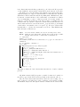
Algorithm 1 processes all variables and prints the basic characteristic intervals in increasing order of upper bounds. In addition to this task, it also identifies
which kind of characteristic intervals the algorithm prints: a Hall interval, a Stable interval or an interval that could contain values of an unstable set. This is
done by maintaining a counter c1 that keeps track of how many variable domains are contained in an interval on the stack. Counter c2 is similar but only
counts the first A variables contained in each sub-characteristic interval A. A
characteristic interval I is a stable interval if c2 is greater than I and might
contain values of an unstable set if c2 is equal to I. We ignore characteristic
intervals with c2 < I since those intervals are not used to define Hall intervals,
stable intervals or unstable sets.
Input : X are the variable domains sorted by non decreasing lower bounds
Result : Prints the basic characteristic intervals and specifies if they are Hall
intervals, stable intervals or contain values of an unstable set
S ← empty stack
push(S, [−∞, ∞], 0, 0)
Add a dummy variable that forces all elements to be popped off of the stack on
termination
X ← X ∪ [max(D) + 1, max(D) + 3]
for x ∈ X do
while max(top(S).interval) < min(dom(x)) do
I, c1 , c2 ← pop(S)
if I = c1 then print “Hall Interval”: I
else if I
< c2 then print “Stable Interval”: I
else if I
= c2 then print “Might Contain Values from Unstable Sets”: I
I , c1 , c2 ← pop(S)
push(I , c1 + c1 , c2 + min(c2 , I
))
I ← dom(x), c1 ← 1, c2 ← 1
while max(top(S).interval) ≤ max(I) do
I , c1 , c2 ← pop(S)
I ← I ∪ I
c1 ← c1 + c1
c2 ← c2 + c2
push(S, I, c1 , c2 )
Algorithm 1: Prints the basic characteristic intervals in a bounds consistent
problem.
Algorithm 1 runs in O(|X|) steps since a variable domain can be pushed on
the stack, popped off the stack, and merged with another interval only once.
Once the basic characteristic intervals are listed in non-decreasing order of
upper bounds, we can easily enforce range consistency on the variable domains.
We simultaneously iterate through the variable domains and the characteristic
intervals both sorted by non-increasing order of upper bounds. If a variable xi
is only contained in characteristic intervals that contain values of an unstable
set, then we remove all characteristic intervals strictly contained in the variable
domain. We also remove from the domain of xi the values whose lower capacity
lv is null. In order to enforce the ubc, we remove a Hall interval H from all
variable domains that is not contained in H.
Removing the characteristic intervals from the variable domains requires at
most O(c|X|) steps where c ≤ |X| is the number of characteristic intervals.
Removing the values whith null lower capacities requires at most O(|X||D|)
instructions but can require no work at all if lower capacities lv are all null or all
positive. If lower capacities are all positive, no values need to be removed from
the variable domains. If they are all null, the problem does not have unstable sets
and only Hall intervals need to be considered. The final running time complexity
is either O(c|X|) or O(c|X| + |D||X|) depending if lower capacities are all null,
all positive, or mixed.
Example: Consider the following bounds consistent problem where D = [1, 6],
lv = 1, and uv = 2 for all v ∈ D. Let the variable domains be dom(xi ) = [2, 3] for
1 ≤ i ≤ 4, dom(x5 ) = [1, 6], dom(x6 ) = [1, 4], dom(x7 ) = [4, 6], and dom(x8 ) =
[5, 5]. Algorithm 1 identifies the Hall interval [2, 3] and the two characteristic
intervals [5, 5] and [1, 6] that contain values of an unstable set. Variable domains
dom(x5 ) to dom(x8 ) are only contained in characteristic intervals that might
contain values of unstable sets. We therefore remove the characteristic intervals
[2, 3] and [5, 5] that are stricly contained in the domains of x5 , x6 , and x7 .
The Hall interval [2, 3] must be removed from the variable domains that strictly
contain it, i.e. the value 2 and 3 must be removed from the domain of variables
x6 and x8 . After removing the values, we obtain a range consistent problem.
5.2
Dynamic Case
We want to maintain range consistency when a variable domain dom(xi ) is modified by the propagation of other constraints. Notice that if the bounds of dom(xi )
change, new Hall intervals or unstable sets can appear in the problems requiring other variable domains to be pruned. We only need to prune the domains
according to these new Hall intervals and unstable sets.
We make the variable domains bounds consistent and find the characteristic
intervals as before in O(t + |X|) steps. We compare the characteristic intervals
with those found in the previous computation and perform a linear scan to
mark all new characteristic intervals. We perform the pruning as explained in
Section 5.1. Since we know which characteristic intervals were already present
during last computation, we can avoid pruning domains that have already been
pruned.
If no new Hall intervals or unstable sets are created, the algorithm runs in
O(t + |X|) steps. If variable domains need to be pruned, the algorithm runs in
O(t + c|X|) which is proportional to the number of values removed from the
domains.
6
Universality
A constraint C is universal for a problem if any tuple t such that t[x] ∈ dom(x)
satisfies the constraint C. We study under what conditions a given gcc behaves
like the universal constraint. We show an algorithm that tests in constant time
if the lbc or the ubc are universal. If both the lbc and the ubc accept any variable
assignment then the gcc is universal. This implies there is no need to run a
propagator on the gcc since we know that all values have a support. Our result
holds for domain, range, and bounds consistency.
6.1
Universality of the Lower Bound Constraint
Lemma 9. The lbc is universal for a problem if and only if for each value v ∈ D
there exists at least lv variables x such that dom(x) = {v}.
Proof. ⇐= If for each value v ∈ D there are lv variables x such that dom(x) =
{v} then it is clear that any variable assignment satisfies the lbc.
=⇒ Suppose for a lbc problem there is a value v ∈ D such that there are less
than lv variables whose domain only contains value v. Therefore, an assignment
where all variables that are not bounded to v are assigned to a value other
than v would not satisfy the lbc. This proves that lbc is not universal under this
assumption.
The following algorithm verifies if the lbc is universal in O(|X| + |D|) steps.
1. Create a vector t such that t[v] = lv for all v ∈ D.
2. For all domains that contain only one value v, decrement t[v] by one.
3. The lbc is universal if and only if no components in t are positive.
We can easily make the algorithm dynamic under the modification of variable
domains. We keep a counter c that indicates the number of positive components
in vector t. Each time a variable gets bound to a single value v, we decrement t[v]
by one. If t[v] reaches the value zero, we decrement c by one. The lbc becomes
universal when c reaches zero. Using this strategy, each time a variable domain
is pruned, we can check in constant time if the lbc becomes universal.
6.2
Universality of the Upper Bound Constraint
Lemma 10. The ubc is universal for a problem if and only if for each value
v ∈ D there exists at most uv variable domains that contain v.
Proof. ⇐= Trivially, if for each value v ∈ D there are uv or fewer variable
domains that contain v, there is no assignment that could violate the ubc and
therefore the ubc is universal.
=⇒ Suppose there is a value v such that more than uv variable domains
contain v. If we assign all these variables to the value v, we obtain an assignment
that does not satisfy the ubc.
To test the universality of the ubc, we could create a vector a such that
a[v] = I({v}) − uv . The ubc is universal iff no components of a are positive. In
order to perform faster update operations, we represent the vector a by a vector
t that we initialize as follows: t[min(D)] ← −umin(D) and t[v] ← uv−1 − uv for
min(D) < v ≤ max(D). Assuming variable domains are initially intervals, for
each variable xi ∈ X, we increment the value of t[min(dom(xi ))] by one and
decrement t[max(dom(xi )) + 1] by one. Let i be an index initialized to value
min(D). The following identity can be proven by induction.
a[v] = I({v}) − uv =
v
t[j]
(1)
j=i
Index i divides the domain of values D in two sets: the values v smaller than
i are not contained in more than uv variable domains while other values can
be contained in any number of variable domains. We maintain index i to be
the highest possible value. If index i reaches a value greater than max(D) then
all values v in D are contained in less than uv variable domains and therefore
the ubc is universal. Algorithm 2 increases index i to the first value v that is
contained in more than uv domains. The algorithm also updates vector t such
that Equation 1 is verified for all values greater than or equal to i.
while (i ≤ max(D)) and (t[i] ≤ 0) do
i ← i+1 ;
if i ≤ max(D) then
t[i] ← t[i] + t[i − 1];
Algorithm 2: Algorithm used for testing the universality of the ubc that increases
index i to the smallest value v ∈ D contained in more than uv domains. The
algorithm also modifies vector t to validate Equation 1 when v ≥ i.
Suppose a variable domain gets pruned such that all values in interval [a, b]
are removed. To maintain the invariant given by Equation 1 for values greater
than or equal to i, we update our vector t by removing 1 from component
t[max(a, i)] and adding one to component t[max(b + 1, i)]. We then run Algorithm 2 to increase index i. If i > max(D) then the ubc is universal since no
value is contained in more domains than its maximal capacity.
Initializing vector t and increasing iterator i until i > max(D) requires
O(|X| + |D|) steps. Therefore, checking universality each time an interval of
values is removed from a variable domain is achieved in amortized constant
time.
7
NP-Completeness of Extended-GCC
We now consider a generalized version of gcc that we call extended-gcc. For each
value v ∈ D, we consider a set of cardinalities K(v). We want to find a solution
where value v is assigned to k variables such that k ∈ K(v). We prove that it is
NP-Complete to determine if there is an assignment that satisfies this constraint
and therefore that it is NP-Hard to enforce domain consistency on extended-gcc.
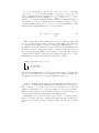
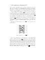
Consider a CNF formula consisting of n clauses ∧ni=1 ∨j Cij , where each literal
Cij is either a variable xk or its negation xk . We construct the corresponding
bipartite graph G as follows. On the left side, we put a set of vertices named
xk for each boolean variable occurring in the formula, and set of vertices named
Cij for each literal. On the right side, we put a set of vertices named xk and xk
(for each variable xk on the left side), and a set of vertices named Ci for each
of n clauses in the formula. We connect variables xk on the left side with both
literals xk and xk on the right side, connect Cij with the corresponding literal
on the right side, and connect Cij with the clause Ci where it occurs. Define the
sets K(l) as {0, degG (l)} for each literal l and K(Ci ) as [0, degG (Ci ) − 1] for each
clause Ci .
For example, the CNF formula (x1 ∨ x2 ) ∧ (x1 ∨ x2 ) is represented as the
graph in Figure 1
C11
C1
{0,1}
C12
C2
{0,1}
C12
x1
{0,2}
C22
x1
{0,2}
x1
x2
{0,3}
x2
x2
{0,1}
Fig. 1. Graph for (x1 ∨ x2 ) ∧ (x1 ∨ x2 )
Let A be some assignment of boolean variables, the corresponding matching
M can be constructed as follows. Match each vertex xk on the left side with
literal xk if A[xk ] is true and with xk otherwise. The vertex Cij is matched
with its literal if the logical value of this literal is true and with the clause Ci
otherwise. In this matching, all the true literals l are matched with all possible
deg(l) vertices on the left side and all the false ones are matched to none. The
clause Ci is satisfied by A iff at least one of its literals Cij is true and hence is not
matched with Ci . So the degM (Ci ) ∈ K(Ci ) iff Ci is satisfied by A. On the other
hand, the constraints K(l) ensure that there are no other possible matchings in
this graph. Namely, exactly one of degM (xk ) = 0 or degM (xk ) = 0 can be true.
These conditions determine the mates of all variables xk as well as the mates of
all literals Cij . Thus, the matchings and satisfying assignments are in one to one
correspondence and we proved the following.
Lemma 11. SAT is satisfiable if and only if there exists a generalized matching
M in graph G.
This shows that determining the satisfiability of extended-GCC is NP-complete
and enforcing domain consistency on the extended-GCC is NP-hard.
8
Conclusions
We presented faster algorithms to maintain domain and range consistency for
the gcc. We showed how to efficiently prune the cardinality variables and test
gcc for universality. We finally showed that extended-gcc is NP-Hard.
References
1. R. K. Ahuja, T. L. Magnanti, and J. B. Orlin Network Flows: Theory, Algorithms,
and Applications. Prentice Hall, first edition, 1993.
2. P. Hall. On representatives of subsets. J. of the London Mathematical Society,
pages 26–30, 1935.
5
3. J. Hopcroft and R. Karp n 2 algorithm for maximum matchings in bipartite graphs
SIAM Journal of Computing 2:225-231
4. ILOG S. A. ILOG Solver 4.2 user’s manual, 1998.
5. C.-G. Quimper, P. van Beek, A. López-Ortiz, A. Golynski, and S. B. Sadjad. An
efficient bounds consistency algorithm for the global cardinality constraint. CP2003 and Extended Report CS-2003-10, 2003.
6. I. Katriel, and S. Thiel. Fast Bound Consistency for the Global Cardinality Constraint CP-2003, 2003.
7. M. Leconte. A bounds-based reduction scheme for constraints of difference. In the
Constraint-96 Int’l Workshop on Constraint-Based Reasoning. 19–28, 1996.
8. J.-C. Régin. A filtering algorithm for constraints of difference in CSPs. In AAAI1994, pages 362–367.
9. J.-C. Régin. Generalized arc consistency for global cardinality constraint. In
AAAI-1996, pages 209–215.
10. J.-C. Régin and J.-F. Puget. A filtering algorithm for global sequencing constraints.
In CP-1997, pages 32–46.
11. K. Stergiou and T. Walsh. The difference all-difference makes. In IJCAI-1999,
pages 414–419.
12. R. Tarjan Depth-first search and linear graph algorithms. SIAM Journal of Computing 1:146-160.
13. P. Van Hentenryck, L. Michel, L. Perron, and J.-C. Régin. Constraint programming
in OPL. In PPDP-1999, pages 98–116.
14. P. Van Hentenryck, H. Simonis, and M. Dincbas. Constraint satisfaction using
constraint logic programming. Artificial Intelligence, 58:113–159, 1992.
15. J.-C. Régin and J.-F. Puget. A filtering algorithm for global sequencing constraints.
In CP-1997, pages 32–46.