1
A CEGAR Tool for the Reachability Analysis of
PLC-Controlled Plants using Hybrid Automata ?
Technical Report
Johanna Nellen, Erika Ábrahám, and Benedikt Wolters
RWTH Aachen University, Aachen, Germany
{johanna.nellen,abraham}@cs.rwth-aachen.de
[email protected]
Abstract. In this paper we address the safety analysis of chemical
plants controlled by programmable logic controllers (PLCs). We consider
sequential function charts (SFCs) for the programming of the PLCs, extended with the specication of the dynamic plant behavior. The resulting hybrid SFC models can be transformed to hybrid automata, opening
the way to the application of advanced techniques for their reachability analysis. However, the hybrid automata models are often too large
to be analyzed. To keep the size of the models moderate, we propose
a counterexample-guided abstraction renement (CEGAR) approach,
which starts with the purely discrete SFC model of the controller and
extends it with those parts of the dynamic behavior, which are relevant
for proving or disproving safety. Our algorithm can deal with urgent
locations and transitions, and non-convex invariants. We integrated the
CEGAR approach in the analysis tool
SpaceEx and present an example.
Keywords: hybrid systems, reachability analysis, CEGAR, verication
1 Introduction
In automation,
programmable logic controllers (PLCs )
are widely used to con-
trol the behavior of plants. The industry standard IEC 61131-3 [25] species
several languages for programming PLCs, among others the graphical language
of
sequential function charts (SFCs ).
Since PLC-controlled plants are often safety-critical, SFC
verication
has
been extensively studied [19]. There are several approaches which consider either
a SFC in isolation or the combination of a SFC with a model of the plant [21,5].
The latter approaches usually dene a timed or hybrid automaton that species
the SFC, and a hybrid automaton that species the plant. The composition of
these two models gives a hybrid automaton model of the controlled plant. Theoretically, this composed model can be analyzed using existing tools for hybrid
?
This work was partly supported by the German Research Foundation (DFG) as
part of the Research Training Group AlgoSyn (GRK 1298) and the DFG research
project HyPro (AB 461/4-1).
2
Johanna Nellen, Erika Ábrahám, Benedikt Wolters
automata reachability analysis. In practice, however, the composed models are
often too large to be handled by state-of-the-art tools.
In this paper we present a counterexample-guided abstraction renement (CEGAR ) [12] approach to reduce the verication eort. Instead of hybrid automata,
we use conditional ordinary dierential equations (ODEs ) to specify the plant
dynamics. A conditional ODE species the evolution of a physical quantity over
time under some assumptions about the current control mode. For example, the
dynamic change of the water level in a tank can be given as the sum of the ows
through the pipes that ll and empty the tank. This sum may vary depending
on valves being open or closed, pumps being switched on or o, and connected
tanks being empty or not. Modeling the plant dynamics with conditional ODEs
is natural and intuitive, and it supports a wider set of modeling techniques (e. g.,
eort-ow modeling).
Our goal is to consider only safety-relevant parts of the complex system
dynamics in the verication process. Starting from a purely discrete model of
the SFC control program, we apply reachability analysis to check the model for
safety. When a counterexample is found, we rene our model stepwise by adding
some pieces of information about the dynamics along the counterexample path.
The main advantage of our method is that it does not restart the reachability
analysis after each renement step but
ability analysis procedure
the renement is embedded into the reach-
in order to prevent the algorithm from re-checking the
same model behavior repeatedly.
Related work
Originating from discrete automata, several approaches have
been presented where
CEGAR is used for hybrid automata [10,11,2]. The work
CEGAR for hybrid automata by restricting the
[15] extends the research on
analysis to fragments of counterexamples. Other works [34,26] are restricted to
the class of rectangular or linear hybrid automata. Linear programming for the
abstraction renement is used in [26]. However, none of the above approaches
exploits the special properties of hybrid models for plant control.
In [13] a
CEGAR verication for PLC programs using timed automata is pre-
sented. Starting with the coarsest abstraction, the model is rened with variables
and clocks. However, this work does not consider the dynamic plant behavior.
A
CEGAR
approach on step-discrete hybrid models is presented in [35],
where system models are veried by learning reasons for spurious counterexamples and excluding them from further search. However, this method was designed
for control-dominated models with little dynamic behavior.
A
CEGAR-based
abstraction technique for the safety verication of PLC-
controlled plants is presented in [14]. Given a hybrid automaton model of the
controlled plant, the method abstracts away from parts of the continuous dynamics. However, instead of rening the dynamics in the hybrid model to exclude
spurious counterexamples, their method adds information about enabled and
disabled transitions.
Several tools for the
reachability analysis
of hybrid automata have been de-
veloped [22,17,24,30,3,20,27,4,33]. We chose to integrate our approach into a tool
that is based on
owpipe-computation. Prominent candidates are SpaceEx [16]
A CEGAR Approach for Reachability Analysis
V1in
P2
3
V2out
T1
max1
V1out
P1
T2
V2in
max2
min1
P1+
P1−
P2+
P2−
min2
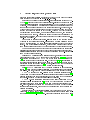
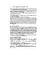
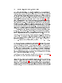
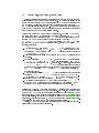
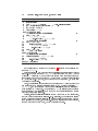
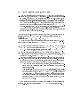
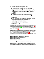
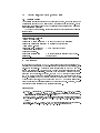
Fig. 1: An example plant and its operator panel
and
Flow*
[9]. For the implementation of our
CEGAR
algorithm we must be
counterexample if an unsafe state is reachable.
Moreover, our modeling approach uses urgent locations in which time cannot
elapse, and urgent transitions whose enabledness forces to leave the current lo-
able to generate a (presumed)
cation. Although
Flow*
provides presumed counterexamples, we decided to
integrate our method into
SpaceEx.
The reason is that
SpaceEx
provides
dierent algorithms for the reachability analysis. Important for us is also the
recently published
PHAVer
scenario [29] that supports urgent transitions and
non-convex invariants for a simpler class of hybrid automata. Furthermore, in [8]
an extension of
SpaceEx
for hybrid automata is presented where the search is
guided by a cost function. This enables a more exible way of searching the state
space compared to a breath- or depth-rst-search.
This paper is an extension of [32]. We made the approach of [32] more ecient
by introducing urgent locations for hybrid automata, dening dedicated methods
to handle urgent locations, urgent transitions and non-convex invariants in the
reachability analysis, and provide an implementation of the proposed methodology. The tool and a technical report containing further details can be accessed
from
http://ths.rwth-aachen.de/research/tools/spaceex-with-cegar/.
Outline
After some preliminaries in Section 2, we describe our modeling ap-
proach in Section 3. In the main Section 4 we present our CEGAR-based verication method. The integration of our CEGAR-based method into the reachability
analysis algorithm, some details on the implementation, and an example are discussed in Section 5. We conclude the paper in Section 8.
2 Preliminaries
2.1
Plants
A simple example of a
two cylindrical tanks
T1
chemical plant
and
T2 ,
is depicted in Figure 1. It consists of
with equal diameters, that are connected by
4
Johanna Nellen, Erika Ábrahám, Benedikt Wolters
pipes. The variables
h1
respectively. Each tank
0 < L < U,
and
Ti
h2
denote the water level in the tanks
is equipped with two sensors
P1
The plant is equipped with two pumps
h2
and increasing
by
k1
P1
and
P2
and a height decrease of
P2
per time unit.
k2
or o:
Pi = 0)
of pump
Pi
T1
to
T2 ,
decreasing
pumps water through a second
k2
per time unit for
h2 .
per time unit for
We overload the meaning of
Pi = 1
T2 ,
which can pump water
pumps water from
pipeline in the other direction, causing a height increase of
h1
and
that detect low and high water levels, respectively.
when the adjacent valves are open.
h1
T1
mini and maxi , at height
and use it also to represent the state (on:
i.
The pumps are manually controlled by the operator panel which allows to
−
+
switch the pumps on (Pi ) or o (Pi ). The control receives this input along
with the sensor values, and computes some output values, which are sent to the
environment and cause actuators to be controlled accordingly, by turning the
pumps on or o. The pumps are coupled with the adjacent valves, which will
automatically be opened or closed, respectively.
We want the control program to prevent the tanks from running dry: If the
water level of the source tank is below the lower sensor the pump is switched o
and the connected valves are closed automatically. For simplicity, in the following
we neglect the valves and assume that the tanks are big enough not to overow.
The
state
of a plant, described by a function assigning values to the physical
quantities, evolves continuously over time. The plant specication denes a set
initial states. The dynamics of the evolution is specied by a set of conditional
ordinary dierential equations (ODEs ), one conditional ODE for each continuous
of
physical quantity (plant variable). Conditional ODEs are pairs of a condition
and an ODE. The conditions are closed linear predicates over both the plant's
physical quantities and the controller's variables; an ODE species the dynamics
in those states that satisfy its condition. We require the conditions to be convex
polytopes, which overlap only at their boundaries. In cases, where none of the
conditional
Example 1.
ODEs
apply, we assume chaotic (arbitrary) behavior.
For the example plant, assume
P1
ϕ2→1 ≡ P2 ∧ h2 ≥ 0
system for h1 :
denote that pump
k1 ≥ k2
and let
ϕ1→2 ≡ P1 ∧ h1 ≥ 0
is on and the rst tank is not empty; the meaning of
is analogous. We dene the following conditional
(c1 , ODEh1 1 ) = ( ϕ1→2 ∧ ϕ2→1 ,
(c2 , ODEh2 1 )
(c3 , ODEh3 1 )
(c4 , ODEh4 1 )
The conditional ODEs for
ḣ1 = k2 − k1 )
ODE
(1)
= ( ϕ1→2 ∧ ¬P2 ,
ḣ1 = −k1 )
(2)
= (¬P1 ∧ ϕ2→1 ,
ḣ1 = k2 )
(3)
= (¬ϕ1→2 ,
h2
ḣ1 = 0)
are analogous.
(4)
A CEGAR Approach for Reachability Analysis
on1
off 1
entry/
entry/
do/
do/
exit/
exit/
open V2in
open V1out
pump P1 on
pump P1 off
close V1out
close V2in
P1− ∨ ¬min1
P1+ ∧ ¬P1− ∧ min1
P1
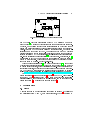
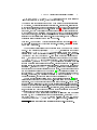
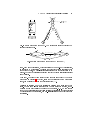
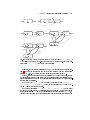
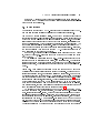
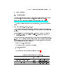
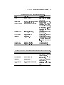
Fig. 2: SFC for pump
2.2
5
Sequential Function Charts
To specify controllers we use
sequential function charts (SFCs ) as given by the
industry norm IEC 61131-3 [25], with a formal semantics as specied in [31] that
is based on [7,6,28] with slight adaptations to a certain PLC application.
Example 2.
Figure 2 shows a possible control program for our example plant.
We specify only the control of
P1 ,
which runs in parallel with an analogous SFC
for the second pump.
Var of typed variables, classied into input, output
state σ ∈ Σ of a SFC is a function that assigns to each
variable v ∈ Var a value from its domain. By PredVar we denote the set of linear
predicates over Var, evaluating to true or false in a given state.
The control is specied using a nite set of steps and guarded transitions
A SFC has a nite set
and local variables. A
between them, connecting the bottom of a source step with the top of a target
step. A distinguished initial step is
active
at start. A transition is
its source step is active and its transition guard from
PredVar
enabled
if
is true in the
current state; taking an enabled transition moves the activation from its source
to its target step. Apart from transitions that connect single steps, also parallel
branching can be specied by dening sets of source/target steps.
A partial order on the transitions denes
priorities
for concurrently enabled
transitions that have a common source step. For each step, the enabled transition
with the highest priority is taken. Transitions are
urgent,
i. e., a step is active
only as long as no outgoing transition is enabled.
Each step contains a set of prioritized
action blocks specifying the actions that
are performed during the step's activation period. An action block
b = (q, a)
is
action qualier q and an action a. The set of all action blocks
using actions from the set Act is denoted by BAct .
a tuple with an
The action qualier
q ∈ {entry, do, exit}1
species when the corresponding
action is performed. When control enters a step, its
1
In the IEC standard, the qualiers
exit.
P 1, N
and
P0
entry and do actions are ex-
are used instead of
entry, do
and
The remaining qualiers of the industry standard are not considered in this
paper.
6
Johanna Nellen, Erika Ábrahám, Benedikt Wolters
ecuted once. As long as the step is active, its
The
exit
do actions are executed repeatedly.
actions are executed upon deactivation.
An action
a is either a variable assignment or a SFC. Executing an assignment
changes the value of a variable, executing a SFC means activating it and thus
performing the actions of the active step.
The execution of a
SFC
on a programmable logic controller performs the
following steps in a cyclic way:
1. Get the input data from the environment and update the values of the input
variables accordingly.
2. Collect the transitions to be taken and execute them.
3. Determine the actions to be performed and execute them in priority order.
4. Send the output data (the values of the output variables) to the environment.
Between two PLC cycles there is a time delay
δ , which we assume to be equal
for all cycles (however, our approach could be easily extended to varying cycle
times). Items 1. and 4. of the PLC cycle implement the communication with the
environment, e. g. with plant sensors and actuators, whereas 2. and 3. execute
the control.
2.3
Hybrid Automata
A popular modeling language for systems with mixed discrete-continuous behav-
hybrid automata. A set of real-valued variables describe the system state.
locations specify dierent control modes. The change of
current control mode is modeled by guarded transitions between locations.
ior are
Additionally, a set of
the
Additionally, transitions can also change variable values, and can be urgent.
Time can evolve only in non-urgent locations; the values of the variables change
continuously with the evolution of time. During this evolution (especially when
entering the location), the location's
invariant
must not be violated.
Denition 1 (Hybrid Automaton [1]). A hybrid automaton (HA) is a tuple
HA = (Loc, Lab,Var, Edge, Act, Inv,Init, Urg)
where
Loc is a nite set of locations;
Lab is a nite set of labels;
Var is a nite set of real-valued variables. A state ν ∈ V , ν : Var → R assigns
a value to each variable. A conguration s ∈ Loc × V is a location-valuation
pair;
Edge ⊆ Loc × Lab × PredVar × (V → V ) × Loc is a nite set of transitions,
where the function from V → V is linear;
Act is a function assigning a set of time-invariant activities f : R≥0 → V to
each location, i. e., for all l ∈ Loc, f ∈ Act (l) implies (f + t) ∈ Act (l) where
(f + t) (t0 ) = f (t + t0 ) for all t, t0 ∈ R≥0 ;
Inv : Loc → 2V is a function assigning an invariant to each location;
Init ⊆ Loc × V is a set of initial congurations such that ν ∈ Inv(l) for each
(l, ν) ∈ Init;
A CEGAR Approach for Reachability Analysis
7
Urg : (Loc ∪ Edge) → B (with B = {0, 1}) a function dening those locations
and transitions to be
urgent
, whose function value is 1.
ordinary dierential equation
ODE ) system, whose solutions build the activity set. Furthermore, it is standard
The activity sets are usually given in form of an
(
to require the invariants, guards and initial sets to dene convex polyhedral sets:
2 by a linear set; if they are
if they are not linear, they can be over-approximated
not convex, they can be expressed as a nite union of convex sets (corresponding
to the replacement of a transition with non-convex guard by several transitions
with convex guards, and similarly for initial sets and location invariants). In the
following we syntactically allow linear non-convex conditions, where we use such
a transformation to eliminate them from the models.
Example 3.
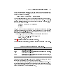
An example HA (without invariants) is shown in Figure 4. A star
∗
in a location indicates that the location is urgent. Similarly, transitions labeled
with a star
∗
are urgent.
The semantics distinguishes between discrete steps (jumps) and time steps
(ows). A jump follows a transition e = (l, α, g, h, l0 ), transforming the current
(l, ν) to (l0 , ν 0 ) = (l0 , h(ν)). This transition, which has a synchronization label α (used for parallel composition), must be enabled, i. e., the guard
g is true in ν and Inv(l0 ) is true in ν 0 . Time steps model time elapse; from a
state ν , the values of the continuous variables evolve according to an activity
f ∈ Act(l) with f (0) = ν in the current location l. Time cannot elapse in urgent locations l, identied by Urg(l) = 1, but an outgoing transition must be
conguration
taken immediately after entering the location. Control can stay in a non-urgent
urgent
transition e, identied by Urg(e) = 1, is enabled, time cannot further elapse in
location as long as the location's invariant is satised. Furthermore, if an
the location and an outgoing transition must be taken. For the formal semantics
and the parallel composition of HA we refer to [1]. The parallel composition of a
set of locations
Loc
yields an urgent location, if
Loc
contains at least one urgent
location. Analogously, the parallel composition of a set of transitions
an urgent transition, if there is at least one urgent transition in
Though the
reachability problem
Trans
is
Trans .
for HA is in general undecidable [23], there
exist several approaches to compute an
over-approximation
of the set of reach-
able states. Many of these approaches use geometric objects (e. g. convex polytopes, zonotopes, ellipsoids, etc.) or symbolic representations (e. g. support functions or Taylor models) for the over-approximative representation of state sets.
The eciency of certain operations (i. e. intersection, union, linear transformation, projection and Minkowski sum) on such objects determines the eciency
of their employment in the reachability analysis of HA.
The basic idea of the reachability analysis is as follows: Given an initial
P0 of initial states (in some representation), a step size τ ∈ R>0
T = nτ (n ∈ N>0 ), rst the so-called ow pipe, i. e., the set
reachable from P0 within time T in l0 , is computed. To reduce the
location l0 , a set
and a time bound
of states
2
For over-approximative reachability analysis; otherwise under-approximated.
8
Johanna Nellen, Erika Ábrahám, Benedikt Wolters
(l0 , P0 )
(l0 , P1 )
(l2 , P4 )
(l0 , P2 )
(l0 , P5 )
(l1 , P3 )
(l1 , P6 )
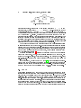
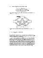
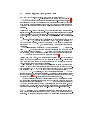
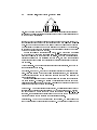
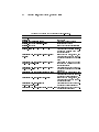
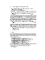
Fig. 3: Example search tree
P1 , . . . , Pn of ow
0 < i ≤ n the set Pi over-approximates the set
of states reachable from P0 in time [(i−1)τ, iτ ] according to the dynamics in l0 .
The intersection of these sets with the invariant of l0 gives us the time successors
of P0 within time T . Finally, we also need to compute for each of the ow
approximation error, this is done by computing a sequence
pipe segments,
where for each
pipe segments (intersected with the invariant) all possible jump successors. This
latter computation involves the intersection of the ow pipe segments with the
transition guards, state set transformations computing the transitions' eects,
and an intersection computation with the target location's invariant; special
attention has to be payed to urgent locations and transitions.
The whole computation of ow pipe segments and jump successors is applied
in later iterations to each of the above-computed successor sets (for termination
usually both the maximal time delay in a location and the number of jumps along
paths are bounded). Thus the reachability analysis computes a
search tree, where
each node is a pair of a location and a state set, whose children are its time and
jump successors (see Figure 3).
Dierent heuristics can be applied to determine the node whose children
will be computed next. Nodes, whose children still need to be computed, are
marked to be
non-completed, the others completed. When applying a xed-point
check, only those nodes which are not included in other nodes are marked as
non-completed.
In our approach, we use the
SpaceEx tool [16], which is available as a stan-
dalone tool with a web interface as well as a command-line tool that provides the
analysis core and is easy to integrate into other projects. To increase eciency,
SpaceEx
2.4
can compute the composition of HA on-the-y during the analysis.
CEGAR
Reachability analysis for HA can be used to prove that no states from a given
unsafe set are reachable from a set of initial congurations. For complex models, however, the analysis might take unacceptably long time. In such cases,
abstraction
can be used to reduce the complexity of the model at the cost of
over-approximating the system behavior. If the abstraction can be proven to be
safe then also the concrete model is safe. If the abstraction is too coarse to satisfy
the required safety property, it can be
rened
by re-adding more detailed infor-
mation about the system behavior. This iterative approach is continued until
either the renement level is ne enough to prove the specication correct or the
A CEGAR Approach for Reachability Analysis
read
cycle
readInput()
comm
t := 0
v := vinit
∗
∗
9
write
t = δ → t := 0; writeOutput()
ṫ = 1
v̇ = 0
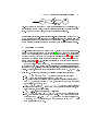
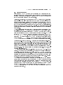
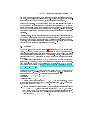
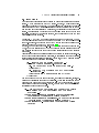
Fig. 4: Hybrid automaton for PLC cycle synchronization and the user input. At
the beginning of each cycle, the input variables (including the user input) are
read. At the end of each cycle, the output variables are written.
model is fully concretized. In counterexample-guided abstraction renement (CEGAR ), the renement step is guided by a counterexample path, leading from the
initial conguration to an unsafe one in the abstraction (i. e., one or more states
on the abstract counterexample path get rened with additional information).
3 Modeling Approach
SFC-controlled plants can be modeled by a HA, built by the composition of several HA for the dierent system components [31]: One HA is used to synchronize
on the PLC cycle time and model the user input (see Figure 4). The control is
modeled by one HA for each SFC running in parallel (see Figure 5). The last
automaton models the plant dynamics according to a given conditional ODE
system (see Figure 7). The parallel composition of these automata gives us a
model for the controlled plant.
v dyn of variables for the physical quantities
sen
v
of variables and expressions represents the
In the models, we use a vector
in the plant dynamics. A vector
input for the SFC, containing control panel requests, actuator states and sensor
values. The input, local and output variables of the SFCs are
Example 4.
v in , v loc
and
v out .
For our example plant, we will use the following encodings:
v dyn = (v1dyn , v2dyn ) with vidyn = hi for the water height in the tanks;
v sen = (v1sen , v2sen ) for the input of the SFC with visen = (∗, ∗, Pi , hi ≥ L, hi ≥
U ), where the rst two entries ∗ encode arbitrary control panel requests Pi+
−
and Pi , Pi is the state of pump i (0 or 1, encoding o or on) and the values
of the sensors
mini
v in = (v1in , v2in )
and
maxi ;
viin = (Pi+ , Pi− , Pi , mi , Mi ) for SFC input variables
sen from above with the control panel requests, the
of v
with
receiving the values
actuator state, and sensor values;
v loc = (), i. e. there are no local SFC variables;
v out = (v1out , v2out ) with v out = (Pion , Pio ) for
the output variables of the
SFC, that control the actuators of the plant. When both commands are
i, i. e. Pion = Pio = 1, then pump i it will be switched o.
on = 1 will cause pump i to be switched on and P o = 1 will
Otherwise, Pi
i
lead to switching pump i o.
active for pump
10
Johanna Nellen, Erika Ábrahám, Benedikt Wolters
PLC Cycle Synchronization. SFCs
running parallel on a PLC synchronize on
reading the input and writing the output. Before each cycle the input is read,
readInput()
where
v sen
stores the current memory image
v in
to
v sen .
The values of
are accessible for all parallel running components and will not change for
the duration of the current cycle. After a constant cycle time
δ,
the output is
written (e. g. commands that control the actuators of the plant are immediately
executed). We model this behavior using the HA shown in Figure 4. We use a
clock
t
with initial value
0
to measure the cycle time. The initial location
is urgent, represented by a star
∗,
will be taken immediately. The transition from
represented by a star
∗,
comm
cycle
thus the outgoing transition to location
cycle
to
comm
is urgent, again
forcing the writing to happen at the end of each cycle.
The synchronization labels
read and write force all parallel running HA that share
those labels to synchronize on these transitions. While time elapses in location
cycle,
the
SFCs
perform their active actions and the dynamic behavior of the
environment evolves according to the specied dierential equations. The ODE
v̇ = 0 expresses that the derivative of all involved discrete variables appearing
sen , v in , v loc or v out is zero. (For simplicity, here we specify the derivative 0
in v
for all discrete variables in the PLC synchronizer model; in our implementation
the SFC variables are handled in the corresponding SFC models.)
Example 5.
For the tank example, we allow arbitrary (type-correct) user input,
∗ to represent a non-deterministically chosen value. (Note, that
∗ has a dierent meaning than the one used for urgency.) Reading the input
readInput() executes Pi+ := ∗, Pi− := ∗, Pi := Pi , mi := (hi ≥ L) and Mi :=
(hi ≥ U ). Writing the output writeOutput() updates Pi := (Pi ∨ Pion ) ∧ ¬Pio .
where we use
this
HA for SFC.
In the HA model of a SFC (see Figure 5), for each step
SFC there is a corresponding location pair in the HA: the location
upon the activation of the step
s
and it is left for location
s
sin
s
of the
is entered
when the input
is read. The execution of the actions is modeled to happen at the beginning of
s to be urgent. The outgoing transitions of
s remains activated then its do actions else
its exit actions and both the entry and the do actions of the next step are
in
executed in their priority order. The location s0 that corresponds to the initial
step s0 denes the initial location of the HA.
the PLC cycle by dening location
s
represent the cycle execution: If
Example 6.
The hybrid automaton model for the SFC for pump
P1
in Figure 2
is modeled by the hybrid automaton depicted in Figure 6.
Plant Dynamics.
ditional
ODEs,
Assume that the plant's dynamics is described by sets of con-
one set for each involved physical quantity. We dene a HA for
each such quantity (see Figure 7); their composition gives us a model for the
plant. The HA for a quantity contains one location for each of its conditional
ODEs and one for chaotic (arbitrary) behavior. The conditions specify the locations' invariants, the ODEs the activities; the chaotic location has the invariant
A CEGAR Approach for Reachability Analysis
11
...
sin
...
Vn
read
s
i=1
entry(s)
);
1 )}
do
(s
1 ),
(s
→
try
g1
,en
(s)
gn
...
sor
t({
exi
t
sn
...
→
);
n
)}
∧g
n
o(s
g i)
1
),d
V n− 1 ¬
(s n
( i= ntry
exit(s)
),e
t(s
exi
t({
do(s)
exit/
s1
...
sor
do/
g1
¬gi → sort({do(s)});
s
∗
entry/
...
sin
1
sin
n
Fig. 5: Hybrid automaton for an SFC. The actions are sorted according to a
specied priority order.
read
oin
1
read
o1
v out := 0
∗
P1+
¬P1−
∧
∧ m1
P1on := 1; P1o := 0
onin
1
on1
v out := 0
∗
P1− ∨ ¬m1
P on := 0; P o := 1
1
1
Fig. 6: Hybrid automaton model of the SFC for pump
true.
P1
Each pair of locations, whose invariants have a non-empty intersection,
is connected by a transition. To assure that chaotic behavior is specied only
for undened cases, we dene all transitions leaving the chaotic location to be
urgent. Note that a transition is enabled only if the target location's invariant
is not violated.
Example 7.
The plant dynamics of the tank example is modeled by the hybrid
automaton in Figure 8. Note that, since the conditions cover the whole state
space, time will not evolve in the chaotic location
Parallel Composition.
(l, 5).
Due to the parallel composition, the models can be very
large. Though some simple techniques can be used to reduce the size, the remaining model might still be too large to be analyzed. E. g. we can remove
from the model all locations with
false
invariants, transitions between locations
whose invariants do not intersect, and non-initial locations without any incoming
transitions.
12
Johanna Nellen, Erika Ábrahám, Benedikt Wolters
l1
ODE1
c1
ln
ODEn
cn
...
ln+1
∗
∗
∗
Fig. 7: Hybrid automaton for the plant dynamics using the conditional
{(c1 , ODE1 ), . . . (cn , ODEn )}
L < h1 < U
ODEs
(l, 1)
ḣ1 = k2 − k1
ϕ1→2 ∧ ϕ2→1
∗
∗
(l, 5)
(l, 2)
ḣ1 = −k1
ϕ1→2 ∧ ¬P2
∗
∗
(l, 4)
ḣ1 = 0
¬ϕ1→2
(l, 3)
ḣ1 = k2
¬P1 ∧ ϕ2→1
Fig. 8: Hybrid automaton model of the plant dynamics for tank
4
T1
with
k1 ≥ k2
CEGAR-Based Verication
In this chapter we explain our
CEGAR
approach for the verication of SFC-
controlled plants. Besides this special application, our method could be easily
adapted to other kinds of hybrid systems.
One of the main barriers in the application of
CEGAR
in the reachability
analysis of hybrid systems is the complete re-start of the analysis after each
renement. To overcome this problem, we propose an embedding of the CEGAR
approach into the HA reachability analysis algorithm : our algorithm renes the
model on-the-y during analysis and thus reduces the necessity to re-compute
parts of the search tree that are not aected by the renement. Besides this
urgent locations and urgent
transitions, which is not supported by most of the HA analysis tools. Last but
advantage, our method also supports the handling of
not least, our algorithm can be used to extend the functionalities of currently
available tools to generate (at least presumed)
abstract counterexamples.
A CEGAR Approach for Reachability Analysis
4.1
The
Model Renement
basis for a CEGAR approach
13
is the generation of a counterexample and
its usage to rene the model. Therefore, rst we explain the mechanism for this
(explicit) model renement before we describe how we embed the renement
into the reachability algorithm to avoid restarts.
Abstraction.
Intuitively, the abstraction of the HA model of a SFC-controlled
plant consists of removing information about the plant dynamics and assuming
chaotic behavior instead. Initially, the whole plant dynamics is assumed to be
chaotic; the renement steps add back more and more information. The idea is
that the behavior is rened only along such paths, on which the controller's correctness depends on the plant dynamics. Therefore, the abstraction level for the
physical quantities (plant variables) of the plant will depend on the controller's
conguration.
active
The abstraction level is determined by a function
location-variable pair
(l, x) a subset
of the conditional
meaning of this function is as follows: Let
H
that assigns to each
ODEs for variable x. The
be the HA composed from the PLC-
without
the plant dynamics. Let l be a
H , x a dynamic variable in the plant model and let active(l, x) =
{(c1 , ODE1 ), . . . , (cn , ODEn )}. Then the global model of the controlled plant
will dene x to evolve according to ODEi if ci is valid and chaotically if none
of the conditions c1 , . . . , cn holds. A renement step extends a subset of the sets
active(l, x) by adding new conditional ODEs to some variables in some locations.
cycle synchronizer and the SFC model
location of
Counterexample-Guided Renement.
The renement is counterexample-guided.
Since the reachability analysis is over-approximative, we generate
presumed coun-
terexamples only, i. e., paths that might lead from an initial conguration to an
unsafe one but might also be spurious. For the renement, we choose the rst
presumed counterexample that is detected during the analysis using a breadthrst search, i. e. we nd
shorter
presumed counterexamples rst. However, other
heuristics are possible, too.
A counterexample is a property-violating path in the HA model. For our
purpose, we do not need any concrete path, we only need to identify the sequence
(l, P )
of nodes in the search tree from the root to a node
where
P
has a non-
empty intersection with the unsafe set. If we wanted to use some other renement
heuristics that requires more information, we could
annotate
the search tree
nodes with additional bookkeeping about the computation history (e. g., discrete
transitions taken or time durations spent in a location).
We rene the abstraction by extending the specication of the (initially
chaotic) plant dynamics with some conditional
ODEs
from the concrete model,
which determines the plant dynamics along a presumed counterexample path.
Our renement heuristics computes a set of tuples
(l, x, (c, ODE)),
where
l
is
a location of the model composed from the synchronizer and the SFC models
without
the plant model,
active(l, x)
a conditional
considered in location l.
x is a continuous variable of the plant, and (c, ODE) ∈
/
ODE for x from the plant dynamics that was not yet
14
Johanna Nellen, Erika Ábrahám, Benedikt Wolters
Possible heuristics for choosing the locations are to rene the rst, the last,
or all locations of the presumed counterexample. The chosen location(s) can be
rened for each variable by any of its conditional
ODEs
that are applicable but
not yet active. Applicable means that for the considered search tree node
the
ODE's
condition intersects with
P.
more then the counterexample path is
(l, P )
If no such renements are possible any
fully rened
and the algorithm terminates
with the result that the model is possibly unsafe.
Building the Model at a Given Level of Abstraction. Let again H be the HA
composed from all HA models without the plant dynamics. Let x1 , . . . , xn be
the continuous plant variables and let active be a function that assigns to each
l of H and to each continuous plant variable xi a subset active(l, xi ) =
{(ci,1 , ODEi,1 ), . . . , (ci,ki , ODEi,ki )} of the conditional ODEs for xi . We build
0
the global HA model H for the controlled plant, induced by the given active
location
function, as follows:
ˆl = (l, l1 , . . . , ln ) with l a location of H and
1 ≤ li ≤ ki + 1 for each 1 ≤ i ≤ n. For 1 ≤ i ≤ n, li gives the index of the
conditional ODE for variable xi and li = ki + 1 denotes chaotic behavior for
xi . We set Urg0 (ˆl) = Urg(l).
The variable set is the union of the variable set of H and the variable set of
The locations of
H0
are tuples
the plant.
e = (l, α, g, f, l0 ) in H , the automaton H 0 has a transition
0 0
with Urg (e ) = Urg(e) for all locations ˆ
l and ˆl0 of H 0
0
whose rst components are l and l , respectively. Additionally, all locations
ˆl = (l, l1 , . . . , ln ) and ˆl0 = (l, l0 , . . . , l0 ) of H 0 with identical rst components
n
1
For each transition
e = (ˆl, α, g, f, ˆl0 )
0
are connected; these transitions have no guards and no eect; they are urgent
0
i lj
= kj + 1
implies lj
= kj + 1
for all
1≤j≤n
(all chaotic variables in
ˆl0
are also chaotic in ˆ
l).
ˆl = (l, l1 , . . . , ln ) are the solutions of the dierential
equations {ODEi,li | 1 ≤ i ≤ n, li ≤ ki } extended with the ODEs of H in l.
The invariant of a location (l, l1 , . . . , ln ) in H 0 is the conjunction of the
invariant of l in H and the conditions ci,li for each 1 ≤ i ≤ n with li ≤ ki .
The initial congurations of H 0 are those congurations ((l, l1 , . . . , ln ), ν)
for which l and ν projected to the variable set of H is initial in H , and ν
The activities in location
projected to the plant variable set is an initial state of the plant.
Dealing with Urgency. The hybrid automaton H resulting from a renement
contains urgent locations and urgent transitions. However, the available tools
SpaceEx
and
Flow*
for the reachability analysis of hybrid automata do not
support urgency. Though a prototype implementation of
PHAVer [29] supports
urgent transitions, it is designed for a restricted class of models with polyhedral
derivatives. To solve this problem, we make adaptations to the reachability analysis algorithm and apply some model transformations as follows.
Firstly, we adapt the reachability analysis algorithm such that no time successors are computed in urgent locations.
A CEGAR Approach for Reachability Analysis
a)
15
b)
(l, . . . , ki +1, . . .)
D
*
(l, . . . , ki +1, . . .)
D
Inv
Inv
c)
(l, . . . , j, . . .)
ODEi,j ∧ D
Inv ∧ ci,j
d)
(l, . . . , ki +1, . . .)
D
Inv ∧ cl(¬ci,j )
(l, . . . , j, . . .)
ODEi,j ∧ D
Inv ∧ ci,j
e)
tz ≥ ε →
(l, . . . , ki +1, . . .)
D
Inv ∧ cl(¬a)
tz := 0
(l, . . . , j, . . .)
ODEi,j ∧ D
Inv ∧ ci,j
tz ≥ ε →
tz := 0
(l, . . . , ki +1, . . .)
D
Inv ∧ cl(¬a)
(l, . . . , j, . . .)
ODEi,j ∧ D
Inv ∧ ci,j
(l, . . . , ki +1, . . .)
D
Inv ∧ cl(¬b)
tz ≥ ε →
tz := 0
(l, . . . , ki +1, . . .)
D
Inv ∧ cl(¬b)
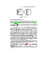
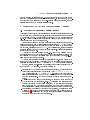
Fig. 9: a) Location
ˆl before the renement; b) Renement using (l, (ci,j , ODEi,j ));
c) Modeling the urgency (over-approximated); d) Modeling non-convex invariants (here:
¬ci,j = ¬(a ∧ b));
e) Zeno path exclusion
Secondly, for the urgent transition in the PLC synchronizer model (see Figure 4), we remove its urgency and set the time horizon
analysis to
δ,
T
i. e., we restrict the time evolution in location
in the reachability
cycle to δ .
Thirdly, for the remaining urgent transitions in the plant dynamics, we use
model transformations to eliminate them: We replace urgent transitions by nonurgent transitions and extend the source locations' invariants by additional conjunctive terms as follows.
Remember that x1 , . . . , xn are the plant variables and let active(l, xi ) =
{(ci,1 , ODEi,1 ), . . . , (ci,ki , ODEi,ki )} be the active conditional ODEs for xi in l.
Let cl(·) denote the closure of a set.
e = ((l, l1 , . . . , ln ), α, g, f, (l, l10 , . . . , ln0 )) in the plant
model is made non-urgent. Additionally, for each variable xi which is chaotic in
0
the source location (li = ki +1) but not chaotic in the target location (li ≤ ki ), we
Each urgent transition
conjugate the invariant of the source location with the negated condition of the
16
Johanna Nellen, Erika Ábrahám, Benedikt Wolters
Inv((l, l1 , . . . , ln )) ∧
cl(¬ci,li0 ). The resulting automaton is shown in Figure 9c.
Note that the elimination of urgent transitions is over-approximative, since in
ODE
V
for
xi
in the target location. Thus the new invariant is
1≤i≤n, li =ki +1, li0 ≤ki
the transformed model we can still stay in a chaotic location after the condition
of an outgoing urgent transition became true. However, in a chaotic location the
dynamics will not enter the inner part (without its boundary) of any active ODE
condition.
Dealing with Non-Convex Invariants.
The above transformation of urgent tran-
sitions to non-urgent ones introduces non-convex invariants unless the conditions
of the conditional
ODEs
are half spaces. Since state-of-the-art tools do not sup-
port non-convex invariants, we again use a transformation step to eliminate
them.
The non-convex invariants can be represented as nite unions of convex sets
NC = C1 ∪ . . . ∪ Ck .
Thus for each location
l
with a non-convex invariant
we compute such a union. This can be obtained by computing the
NC
disjunctive
normal form NC = c1 ∨ . . . ∨ ck , where each clause ci is a conjunction of convex
constraints.
The original location
ants
l
c1 , . . . , ck .
l
is replaced by a set of locations l1 , . . . , lk with invari-
The sets of incoming/outgoing transitions and the dynamics of
are copied for each location
l1 , . . . , l k .
To allow mode switching between the
new locations, we add a transition between each pair of dierent locations from
l1 , . . . , lk
with
true
guard and without eect (see Figure 9d).
Dealing with Zeno Paths.
The construction to resolve non-convex invariants
allows paths with innitely many mode switches in zero time. This is called
Zeno
behavior which should be avoided since both the running time and the
over-approximation might increase drastically.
One possibility to avoid these Zeno behaviors is to force a minimal time
elapse
ε
in each cycle of a location set introduced for the encoding of a non-
convex invariant. To do so, we can introduce a fresh clock tz and modify at least
e = (l, α, g, h, l0 ) in each cycle by an annotated variant (l, α, g ∧
tz ≥ε, h ∧ tz :=0, l0 ). Additionally, we add the dierential equation t˙z = 1 to the
one transition
source location of the annotated transition. The result of this transformation is
shown in Figure 9e. Note that the above transformation eliminates Zeno paths,
but it leads to an
under-approximation
of the original behavior.
Another possibility avoiding the introduction of a new variable is to modify
the reachability analysis algorithm such that the rst ow pipe segment in the
e = (l, α, g, h, l0 ) computes time successors for
jump successors are computed along e. If the
source location of such transitions
and from this rst segment no
model is safe, we complete the reachability analysis also for those, previously
neglected jump successors, in order to re-establish the over-approximation.
CEGAR Iterations.
For the initial abstraction and after each renement we
start a reachability analysis procedure on the model at the current level of abstraction. The renement is iterated until 1) the reachability analysis terminates
A CEGAR Approach for Reachability Analysis
17
without reaching an unsafe state, i. e. the model is correct, or 2) a fully rened
path from an initial state to an unsafe state is found. In the case of 2), the unsafe behavior might result from the over-approximative computation, thus the
analysis returns that the model is
possibly
unsafe.
5 Integrating CEGAR into the Reachability Analysis
5.1
Adapting the Reachability Analysis Algorithm
Restarting the complete model analysis in each renement iteration leads to a recomputation of the whole search tree, including those parts that are not aected
by the renement step. To prevent such restarts, we do the model renement
on-the-y during the reachability analysis and backtrack in the search tree only
as far as needed to remove aected parts.
For this computation we need some additional bookkeeping: During the generation of the search tree, we label all time successor nodes
(l, P ) with the set V
of all plant variables, for which chaotic behavior was assumed in the ow pipe
computation, resulting in a node
(l, P, V ).
In the initial tree, all time successor
nodes are labeled with the whole set of plant variables. Discrete successors are
labeled with the empty set.
We start with the fully abstract model, i. e., with the composition
H
of the
synchronizer and the SFC models, extended with the variables of the plant. Note
that initially we do not add any information about the plant dynamics, i. e., we
allow chaotic behavior for the plant.
We apply a reachability analysis to this initial model. If it is proven to be
safe, we are done. Otherwise, we identify a path in the search tree that leads to
an unsafe set and extend the
active
function to
active 0
as previously described.
However, instead of re-starting the analysis on the explicit model induced by
the extended
active 0
function, we proceed as follows:
Backtracking: When a renable counterexample is found, we backtrack in the
l and variable x with active 0 (l, x)\active(l, x) 6=
∅. We delete all nodes (l, P, V ) with x ∈ V , i. e. those nodes whose conguration contains location l and for which x was assumed to be chaotic in the
tree for each pair of location
owpipe construction. We mark the parents of deleted nodes as not completed.
Model Renement:
After the backtracking, we rene the automaton model
that is used for the analysis on-the-y, by replacing the location(s) with
chaotic behavior in newly rened variables
x
by the locations that result
from the renement. After this modication, we can apply the unchanged
analysis algorithm on the parents of rened nodes to update the search tree.
Reachability Computation:
According to a heuristics, we iteratively apply
Algorithm 1 to non-completed nodes in the search tree, until we detect an
unsafe set (in which case a new renement iteration starts) or all nodes are
completed (in which case the model is safe).
18
Johanna Nellen, Erika Ábrahám, Benedikt Wolters
Algorithm 1: SuccessorComputation
:
input
1
2
3
4
5
6
7
8
9
10
11
12
13
14
15
16
17
18
19
20
SearchTree tree;
Node
Set
Set
V
C
n0 = (l0 , P0 , V0 )
// non-completed node;
in tree;
of variables that are chaotic in l0 ;
of the ODEs of l0 ;
Time horizon
T = mτ ;
l0 is not urgent then
/* compute the flow pipe segments
for i = 1 to m do
Pi := flow (Pi−1 , C, τ );
ni :=tree.addChild(ni−1 , (l0 , Pi , V ));
/* compute jump successors
for i = 1 to m do
foreach transition e = (l0 , α, g, h, l) do
P := h(Pi ∩ g) ∩ Inv(l);
tree.addChild(ni , (l, P, ∅));
for i = 0 to m do
mark ni completed;
if l0 is urgent then
/* compute jump successors
foreach transition e = (l0 , α, g, h, l) do
P := h(P0 ∩ g) ∩ Inv(l);
tree.addChild(n0 , (l, P, ∅));
mark n0 completed;
if
*/
*/
*/
In the following we explain how Algorithm 1 generates the successors of a
tree node
(l0 , P0 , V0 ).
First the algorithm computes the time successors if the location is not urgent
(lines 7-9): The set of states
dynamics
C
within time
τ
flow (Pi , C, τ )
time horizon, and added as a child of
in
l0
reachable from the node
ni
under
is computed for all ow pipe segments within the
ni ,
with the set
V
of the chaotic variables
attached to it. Note that, though we use a xed step size
τ,
it could also
be adjusted dynamically.
Next, the successor nodes of each ow pipe segment
ni
are computed that
are reachable via a discrete transition (lines 10-13). For each transition
(l0 , α, g, f, l),
the set of states
when starting in
tree as a child of
P
e =
e
is computed that is reachable via transition
Pi (line 12). The successor (l, P, ∅) is inserted into the search
ni ; it is labeled with the empty set of variables since no chaotic
behavior was involved (line 13).
Finally, since all possible successors of all
ni
are added to the search tree,
they are marked as completed (lines 14-15). Optionally, we can also mark all new
nodes, whose state sets are included in the state set of another node with the
same location component, as completed. Since the inclusion check is expensive,
it is not done for each new node, but in a heuristic manner.
A CEGAR Approach for Reachability Analysis
If the node
n0
In either case
19
is urgent, only the jump successors are computed (lines 16-19).
n0
is marked as completed since all possible successor state
have been computed (line 20).
5.2
Implementation
We integrated the proposed
CEGAR-approach into the analysis tool SpaceEx.
Some implementation details are discussed in the following paragraphs.
Some SpaceEx Implementation Details. The SpaceEx tool computes the set of
reachable states in so-called iterations. In each iteration, a state set is chosen, for
which both the time elapse and the jump successors are computed. The waiting
list of states that are reachable but have not yet been analyzed, is initialized with
the set of initial states. At the beginning of an iteration, the front element
w
of
T
of
w
the waiting list is picked for exploration. First the time elapse successors
passed list ). Afterwards,
are computed and stored in the set of reachable states (
the jump successors
J
are computed for each
s ∈ T.
These states are added to
the waiting list, as they are non-completed.
In
SpaceEx, the passed
and the
waiting list
are implemented as
FIFO
(rst
in, rst out) queues, i. e., elements are added at the end of the list and taken
from the front.
When either the waiting list is empty (i. e., a xed-point is reached) or the
specied number of iterations is completed, the analysis stops. The reachable
states are the union of the state sets in the passed and the waiting list. If
states
bad
are specied, the intersection of the reachable and the bad states is com-
puted.
Search Tree.
An important modication we had to make in
SpaceEx is the way
SpaceEx
of storing reachable state sets discovered during the analysis. Whereas
stores those sets in a queue, our algorithm relies on a search tree. Thus we added
a corresponding tree data structure. We distinguish between
and
time successor
jump successor
nodes which we represent graphically in Figure 10 by lled
rectangles and lled circles, respectively. The set of initial states are the children
of the distinguished root node, which is represented by an empty circle. Each
node can have several jump and at most one time successor nodes as children.
For a faster access, each jump successor node stores a set of pointers to the next
jump successors in its subtree (dashed arrows in Figure 10).
To indicate whether all successors of a node have been computed, we introduce a
completed
ag. In each iteration, we determine a non-completed tree
node. If its location is non-urgent, we compute its time successors and the jump
successors of all time successors. Afterwards, the chosen node and all computed
time successors are marked as completed. For urgent locations, only the jump
successors are computed. We use
breadth-rst search
(BFS) to nd the next
non-completed tree node. The iterative search stops if either all tree nodes are
completed or the state set of a node intersects with a given set of bad states.
The latter is followed by a renement and the deletion of a part of the search
20
Johanna Nellen, Erika Ábrahám, Benedikt Wolters
δ
e1
e3
δ
e3
δ
e2
δ
e1
δ
e1
e2
e6
δ
e5
Fig. 10: The search tree (empty circle: distinguished root; lled rectangle: jump
successor node; lled circle: time successor node; dashed connections: shortcut
to the next jump successors)
tree (note, that the parents of deleted nodes are marked as non-completed). After this backtracking we start the next iteration with a new BFS from the root
node. If the BFS gives us a node which already has some children then this node
was previously completed and some its children were deleted by backtracking.
In this case we check for each successor whether it is already included as a child
of the node before adding it to the tree.
Renement relies on counterexample paths, i. e. on paths from an initial
to a bad state. To support more information about counterexample paths, we
annotate the nodes in the search tree as follows. Each jump successor node
contains a reference to the transition that led to it, and each time successor
node stores the time horizon that corresponds to its time interval in the owpipe
computation.
Urgent Locations.
Our implementation supports urgent locations, for which no
time successors are computed.
Bad States.
In
SpaceEx, a set of bad (forbidden ) states can be specied by the
user. After termination of the reachability analysis algorithm, the intersection
of the reachable states with the forbidden ones are computed and returned as
output information.
In our implementation we stop the reachability computation once a reachable
bad state is found. Therefore, we perform the intersection check for each node
directly after it has been added to the tree. This allows us to perform a renement
as soon as a reachable bad state is detected.
Renement.
When a counterexample is detected, a heuristics chooses a (set of )
location(s) and corresponding conditional
ODEs
for the renement. We extend
the set of active ODEs and rene the hybrid automaton model on-the-y. Afterwards, the analysis automatically uses the new automaton model and the
backtracked search tree to continue the reachability analysis.
Backtracking.
When the model renement is completed, we delete all nodes
(and their subtrees) whose location was rened. The parents of deleted nodes
A CEGAR Approach for Reachability Analysis
21
are marked as non-completed. This triggers that their successors will be recomputed. Since we use a BFS search for non-completed nodes, rst the successors of such nodes will be computed, before considering other nodes.
Renement Heuristics.
We implemented a command line interface that allows
us to choose the set of locations and corresponding conditional
ODEs
for the
renement manually whenever a counterexample was detected. This provides us
with the most exibility since any strategy can be applied. We plan to investigate several heuristics and to implement automated strategies for the promising
heuristics.
Analysis Output.
In case a counterexample path is detected that is fully rened,
we abort the analysis and output the counterexample path. It can be used to
identify the part of the model that leads to a violation of the specied property.
Otherwise, the analysis is continued until either a xed-point is found or the
number of maximal allowed iterations was computed.
5.3
Example
We use the 2-tank example from Section 2 to illustrate how the implementation
works. Up to now, we used the
PHAVer
scenario of
SpaceEx
for the reacha-
bility analysis since it computes exact results for our model and is much faster
LGG scenario. However, we integrated our
LGG scenario to be able to verify more complex examples in
than a reachability analysis using the
approach into the
the future.
We rst present our integrated
CEGAR method on a two tank model with a
single pump. Afterwards, we show the results for the presented two tank model.
All model les and the
SpaceEx
are available for download at
spaceex-with-cegar/.
Model with a Single Pump.
the second pump
urgent location
Constants:
Pump state:
Continuous vars:
P2 .
version with the integrated
CEGAR
method
http://ths.rwth-aachen.de/research/tools/
First, we model a system of the two tanks without
Initially, the pump
(oin
1 , comm).
P1
is switched o, i. e., we start in the
The initial variable valuation is:
k1 = 1, δ = 3, L = 2, U = 30
P1 = 0
h1 = 7, h2 = 5, t = 0
P1+ = 1, P1− = 0 in the beginning. We want
to prove that the water level of tank T1 will never fall below 2, i. e. we dene the
set of unsafe states as ϕ1 with ϕ1 := h1 ≤ 2.
We assume that the user input is
The rst counterexample is detected by the analysis for an initial user input
P1+ = 1 and P1− = 0, along the location sequence (oin
1 , comm), (o1 , cycle),
(onin
1 , cycle), where h1 behaves chaotic. Thus, the unsafe states are reachable
in
and we rene the location (on1 , cycle) with the rst conditional ODE of h1 ,
which reduces to (P1 ∧ h1 ≥ 0,
ḣ1 = 1).
22
Johanna Nellen, Erika Ábrahám, Benedikt Wolters
When the analysis reaches the location
scribed path, the behavior for
time units, the value of
h1
h1
(onin
1 , cycle)
via the previously de-
is specied, i. e. after a cycle time of three
has decreased from seven to four. Afterwards, the
input reading is synchronized in location
(onin
1 , comm).
We reach again the
(on1 , cycle). For chaotic user input, both location (oin
1 , cycle) and
in
(on1 , cycle) are reachable. If (oin
,
cycle
)
is
analyzed
rst,
a
counterexample
1
is found which can be resolved using the conditional ODE (¬P1 ,
ḣ1 = 0).
in
However, if location (on1 , comm) is processed, time can elapse, which yields
h1 = 1 at the end of the second PLC cycle. A water level below L = 2
location
violates our property. Since the counterexample is fully rened, the analysis
is aborted since the model is incorrect.
The Two Tank Model.
initially in location
Constants:
Continuous vars:
Let us now consider both pumps, which are switched o
in
(oin
1 , o2 , comm).
The initial variable valuation is:
k1 = 5, k2 = 3, δ = 1, L = 1, U = 30
h1 = 5 , h2 = 5 , P 1 = 0 , P 2 = 0 , t = 0
L, i. e. we
ϕ2 := h2 ≤ L.
We want to check that the water level of the tanks is always above
dene the set of unsafe states as
with
ϕ1 := h1 ≤ L
and
in
(oin
1 , o2 , comm), (o1 , o2 , cycle),
+
in
in
(on1 , on2 , cycle) for the initial user input P1 = 1, P1− = 0, P2+ = 1, and
P2− = 0. We rene the last location on the path using (c1 , ODEh1 1 ) = ϕ1→2 ∧
ϕ2→1 , ḣ1 = k2 − k1 ) and (c1 , ODEh1 2 ) = ϕ1→2 ∧ ϕ2→1 , ḣ2 = k1 − k2 ).
in
in
Now, time can elapse in location (on1 , on2 , cycle) and the values of h1 and
h2 are decreased or increased according to the dierential equations. After
The rst detected counterexample is
the rst PLC cycle, we have
ϕ1 ∧ ϕ2
h1 = 3
and
h2 = 7.
Depending on the user input, the locations each pump might be switched on
or o, thus there are four jumps to dierent locations possible. Depending
on the order in which they are analyzed, several renements are neccessary
before the case that both pumps stay switched on is processed.
•
When the rst three locations are processed, counterexamples are detected which can be resolved using those conditional ODEs whose conditions are enabled.
•
With a user input
P1+ = P1− = P2+ = P2− = 0
for the second PLC cycle,
both pumps stay switched on and time can elapse again. Thus, at the
end of the second cycle, we have
h1
is again below
L,
h1 = 1
and
h2 = 9.
Since the value of
we have detected the same counterexample than in
the smaller model with only a single pump. Note that it depends on the
pumping capacity
ki
of the pumps and on the initial values of
hi ,
which
tank can dry out rst.
The models can be corrected by lifting the position of the lower sensors in
the tanks, i. e. for a new sensor position
L0 > L + 2δk1
the models are safe.
A CEGAR Approach for Reachability Analysis
23
6 User Manual
6.1
Getting Started
The Linux binaries of our tool and a benchmark set are available for download
on our website. The content of the Tarball-archive is listed in Table 2.
http://ths.rwth-aachen.de/research/tools/spaceex-with-cegar/
The binary distributable comes in a Tarball archive, which can be extracted
using:
tar xzf spaceex_cegar . tar . gz
The provided Linux binaries have been compiled on a 64bit Ubuntu 12.04 machine. To run the tool via commandline, switch to the location of the executable
and run:
./ spaceex_64bit / spaceex_cegar -- config [ path to config
file ] -m [ path to model file ] -- dynamics [ path to
dynamics file ]
We provide executable bash scripts for our benchmarks in the
I. e. the
CEGAR
benchmark folder.
analysis is automatically started with the correct parameters
by the script. Switch to the location of the bash script, ensure that the script
le is marked as executable by running:
chmod + x run_ { instance }
The benchmark can be executed by running:
./ run_ { instance }
The benchmarks that we provide are listed in Table 1.
Table 1: The benchmarks that we provide.
Benchmark
Manual Con- Script Name
trol
benchmarks/
two_tank_example_single_pump
benchmarks/two_tank_example
none
chaotic
none
chaotic
run_without_user
run_with_chaotic_user
run_without_user
run_with_chaotic_user
24
Johanna Nellen, Erika Ábrahám, Benedikt Wolters
Table 2: The content of the downloadable tar-archive.
File/Folder
LICENCE.txt
README.txt
spaceex_64bit/spaceex_cegar
spaceex_64bit/bin/sspaceex_cegar
spaceex_64bit/lib
benchmarks/two_tank_example_single_pump/
chaotic_user
Description
license le
readme le
bash script to run the tool
executable of the tool
folder with precompiled libraries
folder with the model, cong, and
dynamics le for the two tank example with a single pump with
chaotic user input
benchmarks/two_tank_example_single_pump/
no_user/
folder with the model, cong, and
dynamics le for the two tank example with a single pump without
user
benchmarks/two_tank_example_single_pump/
run_with_chaotic_user
bash script to run the two tank
example with a single pump with
chaotic user input
benchmarks/two_tank_example_single_pump/
run_without_user
bash script to run the two tank example with a single pump without
user input
benchmarks/two_tank_example/chaotic_user
folder with the model, cong, and
dynamics le for the two tank example with chaotic user input
benchmarks/two_tank_example/no_user/
folder with the model, cong, and
dynamics le for the two tank example without user
benchmarks/two_tank_example/
run_with_chaotic_user
benchmarks/two_tank_example/run_without_user
bash script to run the two tank example with chaotic user input
bash script to run the two tank example without user input
A CEGAR Approach for Reachability Analysis
6.2
25
Input Format
Our tool needs three separate input les: The
SpaceEx
system. We did not alter the
gle automata instead of networks. The
model le
describes the analyzed
syntax. However, we only support sin-
conguration le
describes the analysis
dynamics le a set of conditional ODEs is given, that species the dynamics of the
parameters for
SpaceEx
(including initial and forbidden states) and in the
system. All les should be provided as commandline arguments when the tool
is started. In case no dynamics le is given, our tool asks for it when the rst
counterexample was detected.
Model File.
A
SpaceEx
model le describes a network of automata. The in-
put/output behavior between the automata is given by a set of network automata. In general, we adhere to the
ual can be found at the
SpaceEx
SpaceEx syntax for which a detailed man-
homepage [18].
However, we do not support the on-the-y composition of a network of automata.
Thus, we have to restrict the
SpaceEx model le to specify a single automaton
and a single network automaton that denes a single instance of the specied
automaton.
All locations whose name includes
URGENT
are handled as urgent locations. Al-
though time cannot elapse in such a location, it is necessary to provide dierential equations for all continuous variables. Otherwise,
SpaceEx assumes chaotic
behavior as soon as the location is entered.
<! - - Example for an urgent location -->
< location id ="1" name =" loc_URGENT " >
<! - - An invariant might be specified here - - >
< invariant / >
<! - - specify the dynamics for all continuous
variables -->
< flow > var1 ' == 0 & amp ; var2 ' == 0 </ flow >
</ location >
For the renement and the zeno avoidance, the following variables, labels, locations and transitions are needed additionally. These elements should form a
connected component that is not reachable from any other location, i.e. they
are neglected during the analysis. However, we need them to add locations and
transitions during a renement step.
<! - - The following variables and transition labels
are needed for the refinement and the zeno
avoidance -->
< param dynamics =" any " name =" t " controlled =" true "
local =" true " type =" real " d2 ="1" d1 ="1"/ >
< param dynamics =" any " name =" zeno_t " controlled =" true "
local =" true " type =" real " d2 ="1" d1 ="1"/ >
< param name =" copy_transition " local =" true " type ="
label "/ >
26
Johanna Nellen, Erika Ábrahám, Benedikt Wolters
<! - - This location is needed for the refinement -->
< location name =" refinement_loc " id ="1000" >
<! - - Insert flow equations with right - hand side '0 '
for each continuous variable -->
< flow >[ default flows ] & t ' == 1 & zeno_t ' == 0 </
flow >
</ location >
<! - - A transition with guard true and without
assignments is needed for the refinement -->
< transition source ="1000" target ="1000" >
< label > copy_transition </ label >
</ transition >
<! - - The following copy transition is needed for the
under - approximative zeno avoidance -->
< transition source ="1000" target ="1000" >
< label > copy_transition </ label >
< guard > zeno_t >= epsilon </ guard >
< assignment > zeno_t = 0 </ assignment >
</ transition >
Conguration File.
A conguration le species the analysis parameters, a set
of initial and a set of forbidden states. We list some parameters in Table 3 but
refer to the
SpaceEx
homepage [18] for more detailed information.
Our implementation depends on xed values for the conguration parameters
that are given in Table 4.
Dynamics File.
The dynamics of the model are specied in a
.xml
le using
conditional ordinary dierential equations. We restrict the ODEs to be linear
since the LGG scenario of
SpaceEx
does not support non-linear ODEs. The
doctype denition of the dynamics le is given in Figure 11.
The root element of a dynamics le is the
<! ELEMENT
<! ATTLIST
<! ELEMENT
<! ELEMENT
<! ELEMENT
condODEsys tag that species a set of
condODEsys ( condODE ) + >
condODEsys refersTo CDATA # REQUIRED >
condODE ( cond ,( equation ) +) >
cond (# PCDATA ) >
equation (# PCDATA ) >
Fig. 11: Doctype denition of the dynamics le.
conditional ODEs. The attribute
refersTo
species the system model to which
the conditional ODE le belongs, i.e. it should match the analyzed system that
is specied in the model le and marked as the analyzed system in the cong
le.
A CEGAR Approach for Reachability Analysis
Table 3: Some
SpaceEx
27
conguration parameters.
Name
Command
Description
System
system = tanks
The
analyzed
must
be
system
a
network
component.
Initial States
Forbidden States
initially ="(loc(aut)== loc1
& system.var1 == 1)"
forbidden = "h1 <= min1"
Initial location and variable constraints.
Location
and
variable
constraints. If no forbidden states are specied,
a
reachability
is
performed,
analysis
i.e.
counterexamples
no
will
be
detected.
Sampling Time
sampling-time = 0.1
Time Horizon
time-horizon = 4
Discretization step of the
time horizon.
Maximal
time
elapse
in
each iteration.
Iterations
iter-max = -1
Maximal number of analysis iterations. The value
-1 starts an analysis that
runs until a xed point is
found.
Relative Error
Absolute Error
Table 4: The
rel-err = 1.0e-12
abs-err = 1.0e-13
SpaceEx
The relative error.
The absolute error.
conguration parameters that are xed for our tool.
Name
Command
Description
Scenario
scenario = supp
Currently, we only support
the
LGG
Support
Function Scenario.
Representation
directions = box
The
state
set
representation.
Clustering
clustering = 0
Set-Aggregation
set-aggregation = "none"
Currently, the clustering
must be set to 0.
Currently,
the
set-
aggregation must be set
to 0.
28
Johanna Nellen, Erika Ábrahám, Benedikt Wolters
<! - - A conditional ODE system contains a set of
conditional ODEs -->
< condODEsys refersTo =" system " / >
A conditional ODE contains a condition and a non-empty set of linear ODEs.
<! - - A conditional ODE consists of a condition and a
non - empty set of differential equations -->
< condODE / >
A condition is a closed linear predicate over the physical quantities of the plant
and the controller's variables. It is given by a single constraint or a conjunction of
constraints. The comparison operators
==, ≥, ≤ are supported. Note, that strict
operators as well as negations and disjunctions are not supported, since
SpaceEx
cannot handle non-convex constraints in invariants and guards. Boolean variables
var == 1 or var (true ) or with var == 0 or NOT var
false ). An example condition is a >= 1.3 AND a == c AND NOT b.
can be assigned with
(
<! - - A condition is a conjuction of constraints -->
</ cond >
A linear ODE is specied using the following notation:
c' == 3.1a + b.
The
left-hand side contains the primed continuous variable for which the dynamics is
given. The right-hand side contains a linear equation over the discrete variables
of the controller and the continuous variables that model the plant dynamics.
<! - - An equation specifies a linear differential
equation -->
< equation / >
7 Usage
After the analysis is started each time a counterexample is detected, it is printed
on the console. The locations visited along the path are given together with the
information, of this location visited as a jump successor (j) and if time elapse
has been computed (t).
Counterexample path :
{ off1_in_off2_in_control1_comm_URGENT } , j , t
{ off1_URGENT_off2_URGENT_control2_cycle1 } , j , t
{ on1_in_on2_in_control2_cycle$$0 } , j , t
{ on1_in_on2_in_control1_comm_URGENT } , j , t
{ on1_on2_URGENT_control2_cycle } , j , t
{ on1_in_on2_in_control2_cycle$$0 } , j , t
If the dynamics le location was not passed as an initial conguration parameter,
it has to be specied when the rst counterexample is found.
Enter name of conditional ODE XML file :
[ condODEs . xml ]
A CEGAR Approach for Reachability Analysis
29
When a counterexample is detected, you can decide to rene (enter 'r') or to
continue the analysis (enter 'c'). This enables you to apply a set of renements
before you continue the analysis.
What ' s next ? ( R ) efine / ( C ) ontinue :
When
(R)refine is selected, you have to choose a location that has to be rened.
Note, that fully rened locations and urgent locations are not listed. To continue,
enter the corresponding number of the location that should be rened, i.e. to
rene location
loc2, enter '2'.
Choose a location to refine :
1) loc1
2) loc2
Next, you have to choose a conditional ODE that is used to rene the location.
This is done analogously. Note, that only those conditional ODE whose condition
intersects with the invariant of the chosen location and that have not yet been
used to rene this location are shown.
Afterwards, the renement status of the chosen location is updated:
Location : off_1_in_control2_cycle
1:[ X ] , 2:[ -] , 3:[ ]
Table 5 explains the syntax of the renement status.
When
(C)ontinue
was selected, the selected renement is performed and after-
Table 5: The Renement status for a given location.
Notation
Description
i:[X]
indicates, that the i-th conditional ode is marked (or has previously
been used) for renement
i:[-]
indicates, that the i-th conditional ode is not allowed for the renement of the chosen location
i:[ ]
indicates, that the i-th conditional ode is allowed for renement, but
has not been chosen so far
wards, the analysis continues. Note, that the analysis is aborted, if no pair of
location and conditional ODE was marked for renement.
loc is rened, several copies of the location are created. The
loc$$i$, where i indicates the ith copy
original location. Copies with chaotic behavior are named loc$$ineg_j
j indicates the j th chaotic location copy.
When a location
non-chaotic location instances are named
of the
where
30
7.1
Johanna Nellen, Erika Ábrahám, Benedikt Wolters
Analysis Result
The analysis is nished if either a xed point is computed, the maximal number
of iterations is reached or a fully rened counterexample is detected. In the
latter case, it is printed along with the following information:
counterexample detected
Fully refined
At the end of the analysis, a short report is given which includes the following
information:
Message
Fully refined
counterexample detected
after 8 iterations.
Iteration 8 done after 0s
Computing reachable states
done after 9.158s
Performed max. number of
iterations (5)without
finding fixpoint.
Forbidden states are
reachable.
Description
A fully rened counterexample was detected
The number of computed iterations
The overall computation time
A xed point is computed
The reachable states intersect with the forbidden states
8 Conclusion
In this paper we proposed a CEGAR-based framework for the analysis of SFCcontrolled chemical plants that can handle urgent locations and transitions, and
non-convex invariants. We described its implementation in
SpaceEx
and pre-
sented a small example. As future work, we plan to analyze a larger case study
with parallel acting controllers. Although a complex system will aect the running time of the analysis, we expect, that our CEGAR approach will not cause
too much overhead since the analysis is interrupted if a counterexample is detected. Especially when the checked property depends only on a part of the
dynamic plant behavior, we can benet from the CEGAR approach since it sufces to analyze an abstraction instead of the concrete model. Moreover, we will
cover further optimizations of the presented algorithm.
References
1. Alur, R., Courcoubetis, C., Halbwachs, N., Henzinger, T.A., Ho, P.H., Nicollin,
X., Olivero, A., Sifakis, J., Yovine, S.: The algorithmic analysis of hybrid systems.
Theoretical Computer Science 138, 334 (1995)
2. Alur, R., Dang, T., Ivancic, F.: Counter-example guided predicate abstraction of
hybrid systems. In: Proc. of TACAS'13. LNCS, vol. 2619, pp. 208223. Springer
(2003)
3. Asarin, E., Dang, T., Maler, O.: The d/dt tool for verication of hybrid systems.
In: Proc. of CAV'02. LNCS, vol. 2404, pp. 746770. Springer (2002)
A CEGAR Approach for Reachability Analysis
31
4. Balluchi, A., Casagrande, A., Collins, P., Ferrari, A., Villa, T., SangiovanniVincentelli, A.L.: Ariadne: A framework for reachability analysis of hybrid automata. In: Proc. of MTNS'06 (2006)
5. Baresi, L., Carmeli, S., Monti, A., Pezzè, M.: PLC programming languages: A
formal approach. In: Proc. of Automation '98. ANIPLA (1998)
6. Bauer, N.: Formale Analyse von Sequential Function Charts. Ph.D. thesis, Universität Dortmund (2004)
7. Bauer, N., Huuck, R., Lukoschus, B., Engell, S.: A unifying semantics for sequential
function charts. In: In the Final Report of the SoftSpez DFG Priority Program.
LNCS, vol. 3147, pp. 400418. Springer (2004)
8. Bogomolov, S., Donzé, A., Frehse, G., Grosu, R., Johnson, T.T., Ladan, H., Podelski, A., Wehrle, M.: Abstraction-based guided search for hybrid systems. In: Proc.
of SPIN'13. LNCS, vol. 7976, pp. 117134. Springer (2013)
9. Chen, X., Ábrahám, E., Sankaranarayanan, S.: Flow*: An analyzer for non-linear
hybrid systems. In: Proc. of CAV'13. LNCS, vol. 8044, pp. 258263. Springer (2013)
10. Clarke, E., Fehnker, A., Han, Z., Krogh, B., Ouaknine, J., Stursberg, O., Theobald,
M.: Abstraction and counterexample-guided renement in model checking of hybrid
systems. Int. Journal of Foundations of Computer Science 14(04), 583604 (2003)
11. Clarke, E., Fehnker, A., Han, Z., Krogh, B., Stursberg, O., Theobald, M.: Verication of hybrid systems based on counterexample-guided abstraction renement.
In: Proc. of TACAS'03. LNCS, vol. 2619, pp. 192207. Springer (2003)
12. Clarke, E., Grumberg, O., Jha, S., Lu, Y., Veith, H.: Counterexample-guided abstraction renement. In: Proc. of CAV'00. LNCS, vol. 1855, pp. 154169. Springer
(2000)
13. Dierks, H., Kupferschmid, S., Larsen, K.: Automatic abstraction renement for
timed automata. In: Proc. of FORMATS'07. LNCS, vol. 4763, pp. 114129.
Springer (2007)
14. Engell, S., Lohmann, S., Stursberg, O.: Verication of embedded supervisory controllers considering hybrid plant dynamics. Int. Journal of Software Engineering
and Knowledge Engineering 15(2), 307312 (2005)
15. Fehnker, A., Clarke, E., Jha, S., Krogh, B.: Rening abstractions of hybrid systems
using counterexample fragments. In: Proc. of HSCC'05. LNCS, vol. 3414, pp. 242
257. Springer (2005)
16. Frehse, G., Guernic, C.L., Donzé, A., Cotton, S., Ray, R., Lebeltel, O., Ripado, R.,
Girard, A., Dang, T., Maler, O.: SpaceEx: Scalable verication of hybrid systems.
In: Proc. of CAV'11. LNCS, vol. 6806, pp. 379395. Springer (2011)
17. Frehse, G.: PHAVer: Algorithmic verication of hybrid systems past HyTech. Int.
Journal on Software Tools for Technology Transfer 10, 263279 (2008)
18. Frehse,
G.:
An
Introduction
to
SpaceEx
v0.8.
Verimag,
France
http://spaceex.imag.fr/documentation/user-documentation/
introduction-spaceex-27
(2010),
19. Frey, G., Litz, L.: Formal methods in PLC programming. In: Proc. of SMC'00.
vol. 4, pp. 24312436. IEEEXplore (2000)
20. Girard, A., Pappas, G.J.: Approximation metrics for discrete and continuous systems. TAC'07' 52(5), 782798 (2007)
21. Hassapis, G., Kotini, I., Doulgeri, Z.: Validation of a SFC software specication by
using hybrid automata. In: Proc. of INCOM'98. pp. 6570. Pergamon (1998)
22. Henzinger, T.A., Ho, P., Wong-Toi, H.: Hytech: A model checker for hybrid systems. Int. Journal on Software Tools for Technology Transfer 1(1-2), 110122 (1997)
23. Henzinger, T.A., Kopke, P.W., Puri, A., Varaiya, P.: What's decidable about hybrid
automata? Journal of Computer and System Sciences 57(1), 94124 (1998)
32
Johanna Nellen, Erika Ábrahám, Benedikt Wolters
24. Herceg, M., Kvasnica, M., Jones, C., Morari, M.: Multi-Parametric Toolbox 3.0.
In: Proc. of the ECC'13. pp. 502510. Zürich, Switzerland (2013)
25. Int. Electrotechnical Commission: Programmable Controllers, Part 3: Programming Languages, 61131-3 (2003)
26. Jha, S.K., Krogh, B.H., Weimer, J.E., Clarke, E.M.: Reachability for linear hybrid
automata using iterative relaxation abstraction. In: Proc. of HSCC'07. pp. 287300.
LNCS, Springer (2007)
27. Kurzhanskiy, A., Varaiya, P.: Ellipsoidal toolbox. Tech. rep., EECS, UC Berkeley
(2006)
28. Lukoschus, B.: Compositional Verication of Industrial Control Systems - Methods
and Case Studies. Ph.D. thesis, Christian-Albrechts-Universität zu Kiel (2005)
29. Minopoli, S., Frehse, G.: Non-convex invariants and urgency conditions on linear
hybrid automata. In: Legay, A., Bozga, M. (eds.) Formal Modeling and Analysis of
Timed Systems. LNCS, vol. 8711, pp. 176190. Springer International Publishing
(2014)
30. Mitchell, I., Tomlin, C.: Level set methods for computation in hybrid systems. In:
Proc. of HSCC'00. LNCS, vol. 1790, pp. 310323. Springer (2000)
31. Nellen, J., Ábrahám, E.: Hybrid sequential function charts. In: Proc. of MBMV'12.
pp. 109120. Verlag Dr. Kovac (2012)
32. Nellen, J., Ábrahám, E.: A CEGAR approach for the reachability analysis of PLCcontrolled chemical plants. In: Proc. of FMi'14 (2014)
33. Platzer, A., Quesel, J.D.: Keymaera: A hybrid theorem prover for hybrid systems.
In: Proc. of IJCAR'08. LNCS, vol. 5195, pp. 171178. Springer (2008)
34. Prabhakar, P., Duggirala, P., Mitra, S., Viswanathan, M.: Hybrid-automata-based
CEGAR for rectangular hybrid systems. In: Proc. of VMCAI'13. LNCS, vol. 7737,
pp. 4867. Springer (2013)
35. Segelken, M.: Abstraction and counterexample-guided construction of
ω -automata
for model checking of step-discrete linear hybrid models. In: Proc. of CAV'07.
LNCS, vol. 4590, pp. 433448. Springer (2007)