1
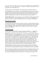
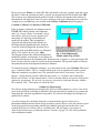
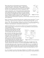
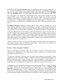
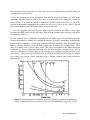
Physics 235
Multichannel Analyzer (MCA) & Gamma-ray Spectroscopy
Purpose: Say you have a radiation detector that puts out an electrical pulse whenever a gamma
ray passes through it. Furthermore, the voltage of that pulse is proportional to the energy of the
gamma ray. You want to keep track of how many gammas are detected as a function of gamma
energy. How do you do it? One way is to use a "Multichannel Analyzer". An MCA is a device
that "bins" voltage signals from a detector and produces a histogram of countrate vs. energy. In
this lab you will learn the basics of using an MCA to analyze detector signals.
Important Preliminary Note on Background Material: The type of radiation detector we will
be using in this course is a phototube that is optically coupled to a scintillating crystal. There is a
great deal of physics involved in these detectors. The MCA spectrum that we will be examining
contains many features that are due to processes that occur in the scintillating crystal. To fully
understand the spectra you'll be studying, you'll need to know the meaning of such terms as:
photoelectric absorption, Compton scattering, Compton shoulder, back-scatter peak, pair
production, double escape peak, single escape peak, and how all these are related to the working
of a phototube detector. Many texts on Modern Physics cover these topics. See for example:
Modern Physics for Scientists and Engineers by S.K. Kim and E.N. Strait, pages 385-391
(check it in the library.) Please make brief notes on the above topics before starting this lab.
You'll be lost without this background information!
Introduction: A single-channel analyzer (SCA) will generate a +5 V logic pulse each time an
input pulse is greater than E but less than E+∆E. A multi-channel analyzer is a succession of
single-channel analyzers whose windows are all the same width and are arranged sequentially in
order of increasing energy. By plotting the count rate of each SCA versus its mean energy
window setting one obtains a spectrum of count rate versus energy.
In an actual MCA, the single-channel analyzers are replaced by a single device called an analogto-digital converter (ADC). The ADC measures the height of each pulse as it comes in and adds a
count to a memory "bin" or "channel" corresponding to that voltage. The voltage range of 0-5V is
typically divided into 512 or more channels. As well as the counts in each channel, the MCA also
records the collection time (often called real or live time) so that count rates can be determined.
The exact correspondence between pulse height and gamma-ray energy depends on many factors
(for example, the type of phototube being used, what voltage it is operated at, how much its
output signal is amplified, the geometry of the scintillating crystal, etc.). Consequently, the MCA
must be calibrated by using an input with known pulse heights.
For example, if a gamma ray spectrum with two peaks
E2
whose energies are known is analyzed by the MCA,
then a correspondence between the energies and the
associated peak channel numbers can be made, as
E1
shown in Fig. 1. This calibration assumes that
all the equipment is strictly linear. For a more precise
calibration, three or more known peaks (up to 96 peaks)
n1
n2
Figure 1. Energy Calibration
1
TS2011,MF2001,RA98
can be used; then a least-squares fit can be made to the calibration points using higher-order
polynomials. If only one calibration point is available, then the MCA automatically assumes a
linear fit that passes through the origin.
The MCA provides for the manipulation of the spectrum display with expand/contract and
linear/logarithmic/sqrt modes and various ways of displaying the data points. In addition, there
are powerful data processing capabilities available in the MCA. The main features are: location of
multiple regions of interest in the spectrum, determination of centroid positions, background
subtraction, energy calibration, and peak identification. While most of these operations can be
performed automatically, it is possible to do some of them under the control of the user.
Using the MCA software: Start the computer and open the Maestro for Windows program on the
desktop. If not deleted, you will see the spectrum previously collected. Go to Acquire on the
main menu and clear the window. The MCA hardware is on a card installed in the computer.
Help from the user’s manual
All multi-channel analyzers have numerous features in common—learning about one model will
help you operate any of them. To get more help on using this program got to the Physics Manuals
website at http:/www.physics.wwu.edu/manuals/. Then under the list of categories, go to Ortec
and open MAESTRO-32 MCA Emulator User’s Manual. You’ll need to refer to this manual
whenever you need help.
Viewing the spectrum
In order to learn more about the MCA, open the file called “sample0.Chn” or “sample01.Chn”
which should be located in the directory K:/Physics/P235/MCA. To do this, go to File, then
Recall and open the above file(s). One of the files is stored in 512 channels while the other one is
stored in 1024 channels. You can Recall these files one by one and view them. The window will
be divided into two to accommodate the two files (spectra). You can close one of the windows
and expand the other to work with. The vertical scale is logarithmic (“Log”). The other possible
scale is linear (“A”). Click and see these scale indicators and observe the spectrum. Select one
(the Log scale is recommended to see possible peaks clearly above the background). The
displayed spectrum was taken in this lab using a Na 22 source and a NaI(Tl) detector. Na 22
decays by emitting a positron and then the resulting isotope very quickly emits a gamma ray,
which is evidenced by the second prominent photo peak to the right. The positron does not travel
far before it meets an electron, and the two annihilate to produce two photons traveling in
opposite directions (to conserve linear momentum). The first and largest peak is due to
annihilation photons. (What is the energy of one of those photons?) Notice that the channel
position of the marker is indicated along with the corresponding number of counts at the bottom
of the window. Try moving the marker by using the mouse and/or the arrow keys on the keypad.
There are many options available for viewing the spectrum, and we will begin by looking at a few
of them. First, put the marker near the top of the photo peak by positioning the mouse pointer
there and then clicking the left mouse button. At times, one wants to see more detail, either for
more accurate positioning of the marker or when there are several peaks close together. The
2
TS2011,MF2001,RA98
small inserted window helps you to zoom in or out. The colors of the spectrum and data points
can be selected by using the Display, References, and Spectrum Colors.
ROIs (Regions of Interest)
The goal in any spectrum analysis is to identify the elements responsible for the radiation and to
determine the activity of each of them. Consequently, the peaks in the spectrum become regions
of interest (ROI) that need to be delineated. Each peak in the spectrum will have one ROI—for
closely spaced peaks the ROIs may overlap. To learn about painting and editing a ROI, go to
Section 4.5 of the MCA Emulator User’sManual.
The ROI status is off by default. Go to ROI and choose Mark. This sets the ROI status to be
active for marking. Next click at the left bottom of the annihilation peak and using the right arrow
on the keyboard move the cursor to the right bottom of the annihilation peak. You can
equivalently do this by placing the marker at the center of the peak and choosing “Insert” from
the keyboard. You will see the peak painted. If you want to clear the painting, go to ROI, then
Clear (“Clear all” for more than one peak painted). An alternate method to paint the peaks is by
using the menu bar Calculate, Peak Search. The software automatically paints peaks that fulfill
the sensitivity criterion. If unwanted peaks are painted, then click on the center of the peak to
locate the marker, then go to ROI and clear. This option sometimes omits peaks that you are after
if they do not meet the sensitivity criterion, so manual painting or using the Insert key are the
better options.
Now locate the marker centered on the top of the annihilation peak, and select ROI from the main
menu. Then paint the area under the peak using the Insert key (observe that the peak is painted
red). If you feel the painted area is wider than the width of the peak you are intending to paint,
then go to ROI/mark and paint it manually by clicking at the left side (bottom) of the peak to
locate the marker, and then use the right arrow key to paint until reaching the right hand side
(bottom) of the peak.
For more facilities and different options to be used read more of the MCA Emulator User’s
Manual.
Exercise 1: Energy Calibration and Peak Identification
To accurately determine the energy of these peaks, go to the Service menu, then Library, Select
Peak. This will open a window containing a list of nuclide, their energy peaks, percentage of
disintegration and half-life. You can sort the library list by nuclide, energy, percent, or life-time.
Search for the Na-22 isotope and record any gamma-ray energies you find. Also write down the
"percent" (a number between 0 and 100 that indicates relative rate of the gamma decays), and the
half-life. When you are done, minimize this window and maximize the MCA window that
contains the Na-22 data (sample0.Chn or sample01.Chn).
If the marker is not already centered on the annihilation peak, locate the marker at the center of
the peak and press Insert to paint it, or paint it manually as explained above. Go to Calculate,
Calibration. The program will ask for the energy of the peak, in keV (not MeV). Enter the
3
TS2011,MF2001,RA98
Energy and, press <Enter> (or click OK). Move the marker to the next (gamma) peak and repeat
the process. After the second peak value is entered, the program will ask for the units click OK.
The system is now calibrated and the marker location is shown at the bottom of the window in
both channels and input (keV) units. If you are not happy with your calibration process and want
a complete new recalibration, you can click on the Destroy Calibration button by going to
Calculate, Calibrate, then Destroy Calibration.
If the spectrum is calibrated, the channel centroid,
FWHM, FW1/xM in channels and calibration
units (e.g., energy), library “best match” energy
and activity, gross area, net area, and net-area
uncertainty are displayed for the ROI peak
marked by the marker. This information is
displayed beneath the Spectrum Window on
the Supplementary Information Line and/or in
a text box inside the Expanded Spectrum View,
at the top of the peak. Both displays are illustrated
in Fig. 2. To remove the text, press <Esc>.
Fig. 2. Peak Info Beneath
The program subtracts the calculated background,
Marker and at Top of Peak.
channel by channel, and attempts a least-squares fit
of a Gaussian function to the remaining data. If unsuccessful, it displays “Could Not Properly Fit
Peak.” If successful, the centroid is based on the fitted function. The reported widths are linearly
interpolated between the background-subtracted channels.
To learn about energy calibration techniques, go to the menu bar and select Calculate. This menu
gives “Sensitivity factor”. This is a criterion for the peak to be acceptable based on the second
difference compared to weighted error. The sensitivity factor can be set between 1 and 5 (an
integer), 1 being the most sensitive (finds the most peaks),.i.e., it includes most small peaks.
Please read section 4.3 of the manual on this. Close or clear the window and you are ready for the
gamma ray spectroscopy. If you wish, you can save your work in your home directory with the
file extension “Chn”. You cannot save on the K: drive
Gamma-ray Spectroscopy
We will now begin collecting and analyzing the spectra of actual gamma-ray sources. One of the
goals of the lab will be to identify an unknown source by measuring its gamma-ray spectrum and
comparing this with data in published isotope tables. We will also investigate the absorption of
gamma rays by matter.
A word of caution: It is absolutely imperative to understand the physics involved in a
phototube/scintillator detector before trying to interpret spectra. Please review the reference given
on the first page before proceeding with this lab. Another good reference for this lab is your
textbook Experiments in Modern Physics by Melissinos. All of Chapter 8 is devoted to a
discussion of various types of radiation detectors. Section 8.4 (page 333-344) deals specifically
with scintillation counters.
4
TS2011,MF2001,RA98
Most isotopes that are used for gamma-ray measurements have
associated beta particles in their decay schemes. A typical decay
scheme for an isotope, as shown in Fig. 3, will include beta decay to a
particular level in an adjacent isotope followed by one or more gamma
emissions as the residual nucleus de-excites to its ground state. Any
electrons emitted by the source will be absorbed by the aluminum light
shield surrounding the detector’s scintillator material and therefore will
not be counted at all. The gamma rays, however, are quite penetrating
and will easily pass through the shield. In this experiment, you will set
Figure 3 Cs Decay.
up and calibrate the spectrometer using Na-22, following which you will
attempt to identify an unknown gamma-ray source. Afterwards, you
will investigate the penetration power of gamma rays in lead absorbers and measure the dead time
of the spectrometer.
Before you begin, take a look in the Table of Isotopes available in the lab and find the 137Cs decay
shown above. Careful study will reveal that there is another pathway through which 137Cs can
decay to 137Ba. What is that pathway? Find the decay scheme for 22Na. Is there more than one
pathway for it? Also look on the Chart of Nuclides found on the wall in the lab and find 137Cs and
22
Na and see what information is contained there about their decays.
With the introduction above, you are now in a position to carry out your own experiment on
different isotopes. However, first you need to re-do the energy calibration of your spectrometer
set up using Na22 isotope.
To do this, set up the electronics according to
the arrangement shown in Fig.4 to the right
(Important safety note: Be sure to use one of
the special high-voltage cables with a longerthan-usual barrel for the high voltage connection.
Please ask someone if you can't find one of these
special cables. Using a regular BNC connector
is dangerous!) The bi-polar output of the
amplifier should be used (if it has one) with the
leading edge positive. There are two parameters
that ultimately determine the overall gain of the
system: the high voltage that is furnished to the photoFigure 4 Schematic for γ Spectrometer.
multiplier tube and the gain of the linear amplifier.
The gain of the phototube is largely dependent upon its high voltage. The high-voltage value
depends on the photo tube being used. You will be using the Harshaw NaI(Tl) detector along
with a Fluke high-voltage supply. Set the latter for about +700 volts (never exceed 1000 volts)
and adjust the amplifier gain to the middle of its range. Be sure to record the gain (both coarse
and fine) of the amplifier and high voltage settings in your lab notebook. Having these numbers
on hand will allow you to continue the experiment on another day without having to do a new
calibration curve.
Use a Na-22 gamma-ray source for the energy calibration (as in the MCA exercise experiment).
Put the source in the smaller cradle in the holder which has been provided. Position the holder so
5
TS2011,MF2001,RA98
that the other end butts up against the front of the phototube—the source should then be about 5
cm in from the detector. Observe the amplified pulses from the detector on the oscilloscope. The
vast majority of them should be 2-6 volts high, and clipping of pulses should not be a frequent
event (a few are OK). (Do you know what is meant by clipping?) Adjust the amplifier gain to
achieve a reasonable distribution of pulse heights (note: the analyzer will accept up to 10-volt
pulses).
Click on the Maestro shortcut on the desk-top to open it (if you have already closed the window
from the MCA exercise). Since the NaI crystal peaks are quite broad, you do not need many
channels—512 or 1024 will do. You can increase or decrease the number of channels by clicking
on the “zoom out” or “zoom in” in the menu bar.
To adjust the amplifier gain so that the peaks occupy most channels but are still on scale, you will
need to take some short sample spectra. Select what seems like a reasonable (short) collection
time by going to the Acquire menu, then MCB properties and choosing Presets, select Live
Time as the Preset Type and type in a Preset Value of 60 seconds. The Pulse Height Analysis
(PHA) window is on the upper right corner of the window to monitor and register the Real Time,
Live Time, and percentage Dead Time. Record them and explain what they represent. Set the
vertical scale to Log and go to “Acquire”, then Start. Depending upon the resulting spectrum,
adjust the amplifier gain up or down so that the entire spectrum occupies most of the 512 or 1024
channels, which are available. When you are satisfied with your setup, clear the spectrum and
reset the Live Time for a sufficiently long period so as to accurately determine the centroids of the
peaks. Then start a normal collection.
Once a good spectrum has been accumulated, stop acquiring and save the data in your home
directory and do an energy calibration following the procedure that you learned while doing the
MCA exercise. Save your data with file extension ”Chn” in your directory. You can also print it
by opening it in WinPlots (see section 7.1 of the manual about WinPlots). To start WINPLOTS,
click on Start on the Windows Taskbar, then Programs, MAESTRO 32, and WinPlots. The
spectrum files are associated with WINPLOTS by the installation program, so double-clicking on
a spectrum filename within Windows Explorer will start WINPLOTS and display that spectrum
too. You can smooth your spectrum once you have saved it in the buffer (but not necessary for
now).
Finally check the effect of putting lead bricks or lead sheets around the source/detector. Clear the
spectrum and surround the source/detector with lead sheets. Collect the data again on Na-22 for
about the same duration and same geometry as when there were no lead sheets. What effect does
this have on the peaks (all peaks that are visible) of the spectrum? Which of the peaks is most
affected by the leads? Explain why.
Exercise 2: Analysis of the Energy Spectrum of Known and Unknown Gamma Sources
Delete all the ROIs and clear the spectrum of Na22 you collected, but do not clear the energy
calibration or close the Maestro program. Closing the window will eliminate your energy
calibration. Do not change the geometry and amplifier settings. Take the Na22 source and put it
away from the detector (put it back in the sources storage).
6
TS2011,MF2001,RA98
(a) Cs-137, Co-57 and Co-60 Spectra: Run the measurement for the energy spectrum for Cs137, Co-57 and Co-60. Click on the prominent peak(s) and read the corresponding energy at the
bottom of the window with the corresponding channel number and counts. Go to the Calculation
menu, then Peak Info. Take a note of the information displayed in a box above the peaks. Go to
the isotope library and confirm the corresponding energy of the peak(s) for each of the three
isotopes. Make a table of the peak values (keV) for the Gamma ray, Compton edge and
backscatter and compare to expected (theoretical) values as well as percentage error (please
research and try to understand what the Backscatter and Compton peaks are and their source).
Save your data in your directory. Use WinPlots to print the results. Clear the window but do not
close it.
(b) Unknown Source(s): Obtain the mystery gamma source (enclosed in black tape; do not
remove the tape) from the radioactive source storage area and use it to replace the last source you
used (which should be moved well away from the detector). The geometry should be the same as
in the previous exercise. Accumulate a spectrum for a period long enough to accurately locate all
of the peaks, Backscatter and Compton edge. After the collection has stopped, note the energy of
all peaks. Compare these energies with the isotope library energies to deduce what the mystery
source is. Remember that the sources you are looking at has been in our lab for at least 10 years.
Thus, it does not contain any isotopes with very short half-lives. Include a copy of the spectrum in
your notebook and be sure to identify all the features (Compton edges, Photopeaks, Backscatter
peaks, etc.) by hand or by using Word.
After the isotope(s) has (have) been correctly identified, record the energies of the gamma rays,
their relative strengths, and the lifetime(s). Also include a sketch of the decay scheme (do
research on this) for the isotope in your notebook.
Exercise 3: Mass Absorption Coefficients
What is an absorption coefficient? Make sure you know the answer to this question before
continuing! See Melissinos, or any other modern physics textbook for a discussion of the
absorption of radiation by matter.
The total-mass absorption coefficient can be measured with a gamma-ray spectrometer. In this
experiment, you will measure the number of gamma rays that are absorbed when lead sheets are
placed between the source and the detector. By varying the thickness of the absorber, it is
possible to measure the mass absorption coefficient. Since Na-22 has two well-defined peaks in
its spectrum, one can determine this coefficient for two different energies at the same time.
1. Return the mystery source to the radioactive storage area and place the Na-22 source in front of
the NaI(Tl) detector with the same geometry as used previously. Go to “Acquire”, MCB
properties and set the Live Time to 60 seconds and start a collection. Paint the ROIs for the
photo and annihilation peaks. If the combined counts in these peaks are not adequate, then
increase the Live Time and perform another collection. Once a satisfactory count level is attained,
record the absorber thickness and NET counts in each ROI in a table constructed for purpose of
7
TS2011,MF2001,RA98
this experiment. Also record the Live Time that you used to collect the data so that counts per
second can be calculated later.
2. Clear the spectrum and place the thinnest lead absorber from the absorber set (A-E) in the
adjustable slot immediately in front of the source (you may need to use some putty to hold the
slider in place). You should be careful to maintain the position of the source just as it was in the
previous measurement. Accumulate the spectrum for the same period as in step 1 above. Record
the absorber thickness and NET counts in both peaks in your table.
• Clear the spectrum and insert the next thickest piece of lead in the holder. Once again
determine the NET counts for the same time. Repeat in this fashion until you have used all the
lead absorbers in the set.
In your notebook give a qualitative description of the effect of the lead absorbers upon the
energies and number of gamma rays reaching the detector. To make it quantitative, normalize the
count rate (R) for thickness x, to the gross count rate (R0) for no absorber. Plot the natural log of
R/R0 vs. absorber thickness in cm for both energies and determine the resulting slopes. Also
make an estimate of the error in these slopes. The slopes correspond to the linear absorption
coefficient, µx. A mass absorption coefficient may also be defined for a material by µm = µx /ρ
where ρ is the material's density. What are the advantages of reporting absorption in terms of µm
instead of µx? Using your slopes calculate the mass absorption coefficient (in cm2/mg) for gamma
rays at these two energies (along with their errors). Finally, compare your results with those
plotted in Fig. 5.
Figure 5. Linear absorption coefficients of several elements as a function of gamma ray
energy. (taken from Introductory Nuclear Physics by David Halliday, page 143, (1955))
8
TS2011,MF2001,RA98