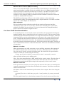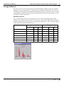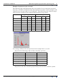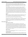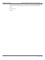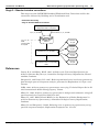
1
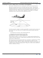
INTREPID User Manual
Library | Help | Top
Multi-channel gamma ray spectrometric processing (C07)
1
| Back |
Multi-channel gamma ray spectrometric processing (C07)
Top
Until relatively recently only large organisations with substantial research resources
could perform multi-channel spectra processing. This processing was therefore not
always available to end-users.
INTREPID has a tool for processing multi-channel spectra as well as the traditional
tool for correcting windowed data. This makes multi-channel processing a routine
operation, well within the resources of any organisation.
This cookbook describes radiometric processing practice.
For practical exercises, see:
•
Calibration gamma ray spectra processing (C07a)
•
Radiometrics processing (C07b)
Background theory
The radiometric component of a geophysical survey commonly includes Multi-channel
Gamma Ray Spectra.
Each data point on a survey line includes
•
Multi-channel spectra
•
Raw windowed data from regions of interest in the spectrum and
•
Ancillary data.
Tip: A data point (sample point) is a set of recorded observations for a single
location. It corresponds to a single record in an INTREPID line dataset. Each
field in the dataset has a value for the data point (or set of values in the case of a
multiband (multi-channel) field).
Tip: A windowed data field contains the sum of counts over a range (window) of
energies. We obtain this by summing the counts over the range of the channels
corresponding to the energy window. For example, an IAEA defined Potassium
window field in a live time-corrected and energy calibrated spectrum will contain
the sum of counts from 1.37MeV to 1.57MeV (channels 116–133). (The IAEA is the
International Atomic Energy Agency, which collects and disseminates information
on gamma ray spectrometer methods).
Library | Help | Top
© 2012 Intrepid Geophysics
| Back |
INTREPID User Manual
Library | Help | Top
Multi-channel gamma ray spectrometric processing (C07)
2
| Back |
Summing the counts: sample area, accumulation and integration
We measure radiometric data by counting pulses detected by the spectrometer.
The pulses originate from the area of ground under the aircraft. The following
illustration shows the area under the aircraft from which pulses may originate. A
significant radioactive anomaly may not be immediately under the aircraft, yet
contribute to the count. There is thus a limitation on the ability of an airborne
radiometric survey to precisely resolve radiometric sources.
In order to provide a sample to examine statistically we need to sum the counts over
time periods. We sum counts over two different time periods during radiometric
processing:
•
Accumulation of counts for a data (sample) point and
•
Integration time for multi-channel corrections.
Accumulation of counts for a data (sample) point
During initial recording, we sum the counts over a sample period (traditionally one
second). The sum of counts for a sample period corresponds to the counts for one data
point in the resulting dataset.
The illustration above showing the sample area is therefore a simplification. During
the sample period the aircraft will travel. The length of the sample area will
therefore exceed 150 m. Moreover, different parts of the sample area will supply data
at different times during the sample period. This places a limit on the resolution of
airborne radiometric surveys.
Library | Help | Top
© 2012 Intrepid Geophysics
| Back |
INTREPID User Manual
Library | Help | Top
Multi-channel gamma ray spectrometric processing (C07)
3
| Back |
Integration time
During multi-channel corrections, e.g., Radon background removal, we need to use
samples consisting of the sum of the counts over several data points. This is
generally because the count rate in a single sample is too low or too variable to be
statistically significant. This number of data points is the integration period or
bunch size. For NASVD and MNF corrections, the data is typically summed on a
line-by-line or a flight-by flight basis.
For the case of Radon removal, the length of the integration period is a compromise
between obtaining sufficient response and how localised we require to correction to
be. When the correction required is highly localised, we require a small integration
period to perform the correction as accurately as possible. The disadvantage with a
small integration time is that it will degrade the data by introducing statistical noise.
Extracting windowed data
You can process the spectra to provide windowed data for map making and
interpretation. The corrected windowed data obtained from the multi-channel
spectra are superior to the windowed data directly recorded by the Gamma Ray
Spectrometer. This is largely because processing options are available for the multichannel data which cannot be applied to windowed data only.
The illustration below shows a typical multi-channel spectrum and the positions of
the standard IAEA defined windows and the gamma ray peak (Bi214 at 0.609MeV)
associated with Radon.
Library | Help | Top
© 2012 Intrepid Geophysics
| Back |
INTREPID User Manual
Library | Help | Top
Multi-channel gamma ray spectrometric processing (C07)
4
| Back |
Steps in the process
The correction process for multi-channel spectra includes:
•
Spectral noise reduction, using either the NASVD or MNF method.
•
Live time / Dead time
•
Drift (Energy Calibration)
•
Cosmic and Aircraft background
•
Radon background.
These corrections may either be carried out together in the one process, or as separate
processes. The spectral noise reduction is by far the most CPU intensive step in the
correction process.
After the spectral smoothing it is normal to store a copy of the smoothed spectra for
input to the remaining multi-channel corrections. After the multi-channel
corrections it is normal to create new windowed data.
The sequence of the corrections is important. It is essential to carry them out in the
order that they appear in the following sections. The correction procedures follow
closely the methods outlined in the reports by IAEA (1991) and Grasty and Minty
(1995). This introduction contains only a brief summary of the procedures. Consult
the reports for more detailed discussion.
Library | Help | Top
© 2012 Intrepid Geophysics
| Back |
INTREPID User Manual
Library | Help | Top
Multi-channel gamma ray spectrometric processing (C07)
5
| Back |
Spectral Noise Reduction
INTREPID has two methods for noise reduction applied to raw gamma-ray spectra.
They are the Noise Adjusted Singular Value Decomposition (NASVD) and the
Maximum Noise Fraction (MNF) methods.
Both methods rely on Principal Component type analysis to extract the dominant
spectral shapes from a dataset. The highest order Principal Components are used to
reconstruct new spectra that retain most of the original coherent signal, but a
significantly reduced noise component. The two methods are very similar both
mathematically, and in the way they are applied to radiometric data. They differ
mainly in how they normalise the raw input spectra for noise before the PC analysis.
The two main parameters which control the output for both NASVD and MNF are the
number of PC components to keep, and whether the integration, or stacking, of the
individual spectra is performed on a line-by-line or a flight-by-flight basis prior to PC
analysis. Currently the INTREPID v3.7 implementation of NASVD only allows
spectra integration on a line-by-line basis. The MNF method allows both.
Noise-Adjusted Singular Value Decomposition (NASVD) smoothing
You can substantially enhance the signal to noise ratio of the multi-channel spectra
using Noise-Adjusted Singular Value Decomposition (NASVD) as described by
Hovgaard and Grasty (1997). Using this method you perform a general linear
transformation of groups of spectra (a whole line), using NASVD to compute the
different spectral shapes that make up the measured multi-channel spectra. You can
then create new multi-channel spectra by recombining the statistically significant
spectral components. Each spectral component contributes an unequal amount to the
features observed in the measured multi-channel spectrum, until a point is reached
where the spectral components represent only noise.
For instance, the 1st spectral component is the spectral shape that represents most of
the features in the measured multi-channel spectra. The 2nd spectral component
represents those features not described by the 1st spectral component, etc.. If you
exclude from the recombination those spectral components that do not represent
significant features in the measured multi-channel spectra, the resulting
reconstructed multi-channel spectra will have a much larger signal to noise ratio
than the measured multi-channel spectra.
In theory, for a proplerly functioning system, just six components are needed to
capture the physics of the measurement system, We recommend that you use eight
for safety.
Note that NASVD smoothing can work on a line by line basis.
Boost the signal stats option
For every sample, a portion of the before and after spectra is added to the observed
signal. As there is overlapping of the footprints, this gets higher counts into the
higher energy channels and so you give the least squares solver a better signal/noise
starting position. This results in a less noisy end product.
Library | Help | Top
© 2012 Intrepid Geophysics
| Back |
INTREPID User Manual
Library | Help | Top
Multi-channel gamma ray spectrometric processing (C07)
6
| Back |
The following illustration, from Hovgaard and Grasty (1997), shows the first eight
components of a group of measured multi-channel spectra.
Library | Help | Top
© 2012 Intrepid Geophysics
| Back |
INTREPID User Manual
Library | Help | Top
Multi-channel gamma ray spectrometric processing (C07)
7
| Back |
Maximum Noise Fraction (MNF) smoothing
Green et al. (1988) developed a general method for minimising (or maximising) the
noise fraction when a sample of noise is available. Lee et al. (1990) describe a noiseadjusted principal component method that is similar to the MNF transform. Their
method consists of two transforms: the first transforms the data to unit error
variance in each channel with no covariance between channel count-rate errors; the
second is a standard PC transform.
The MNF transformation of Green et al. (1988) combines a data-whitening
transformation and a PC transformation into a single transform. It works on all the
spectra for a whole flight, not line by line.
Noise reduction
We have had best noise reduction results by pre-sorting all spectra into bins,
classified by ratios. We use 10–15 bins. At the time of writing, the code for this
method is available, but not released. If you are interested in using this method,
please contact our technical support service.
Live time / Dead time Normalisation
It is normal practice to convert the counts measured by the spectrometer during the
nominal sample time to normalised units of counts per second. This accounts for the
Gamma Ray Spectrometer instrument's two-stage measurement technique. After the
instrument detects an incoming gamma ray, it measures the energy of the detected
pulse. During this measurement phase the spectrometer suspends pulse detection.
As the number of detections increases, the proportion of the nominal sample time
devoted to energy measurement increases, leaving less time for detection. The loss of
time available for detection is called the Dead time. There are two different methods
of correction.
Method 1: Live time
Many spectrometers are able to measure, as an ancillary parameter, the amount of
the nominal sample time devoted to pulse detection. This parameter is called the
Live time and is usually recorded in milliseconds. We normalise the spectrometer
counts to counts per second using the formula
Counts_per_second = (1000.0 / measured_live time) * measured_counts(1)
where all units of time are in milliseconds.
Note : Live time normalisation is NOT applied to the cosmic counts. For this class of
spectrometer it is usual to apply a fixed system dead time (the time taken for the
instrument to perform other processing tasks) separately to the cosmic counts.
Method 2: Dead time
If the spectrometer used in your survey does not measure Live time, we normalise the
counts by computing a Live time from the Dead time constant. Dead time usually has
units of microseconds.
We find its value in the instrument specifications, then compute Live time using the
formula
computed_live time = dead time_per_pulse * total_number_of_counts_measured
(2)
We then apply formula (1), substituting computed_live time for measured_live time.
Library | Help | Top
© 2012 Intrepid Geophysics
| Back |
INTREPID User Manual
Library | Help | Top
Multi-channel gamma ray spectrometric processing (C07)
8
| Back |
Energy Calibration
We may need to correct the spectra for instrument drift and/or remap the existing
channels to standard positions. This is known as Energy Calibration. It involves
identifying the locations of standard photopeaks in the raw spectrum, then creating
an adjusted (or calibrated) spectrum by interpolation from the raw positions to the
standard (or ideal) positions.
Standard spectrum
For a standard spectrum measured from 0.0 to 3.0 MeV and digitised into 256
channels (0 to 255) each channel has a range of 11.71875 keV. The IAEA standard
windows and the gamma ray peak associated with Radon in such a spectrum appear
in the following table and illustration.
Window
Library | Help | Top
Energy Range (MeV)
Channel Range
Start
End
Start
End
Spectrum
0.0
3.0
0
255
Total Count
0.41
2.81
33
238
Radon
0.58
0.64
0.609
49
54
51
Potassium
1.37
1.57
1.46
116
133
124
Uranium
1.66
1.86
1.76
140
158
150
Thorium
2.41
2.81
2.605
205
238
222
© 2012 Intrepid Geophysics
Peak
Peak
| Back |
INTREPID User Manual
Library | Help | Top
Multi-channel gamma ray spectrometric processing (C07)
9
| Back |
Example of spectrum to be corrected
The following table and illustration show an example of a raw spectrum measured
from 0.0 to 3.0 MeV and digitised into 236 channels (0 to 235). In this example, each
channel has an energy range of 12.711864 keV. The table shows the channel ranges
which must be mapped to the standard IAEA window energy limits.
Window
Energy Range (MeV)
Channel Range
Start
End
Start
End
Spectrum
0.0
3.0
0
235
Total Count
0.41
2.81
31
221
Radon
0.58
0.64
0.609
45
49
47
Potassium
1.37
1.57
1.46
107
123
114
Uranium
1.66
1.86
1.76
129
145
137
Thorium
2.41
2.81
2.605
188
221
204
Peak
Peak
If we energy calibrate the raw spectrum in the example above, we will
•
Part of Spectrum
From Channel
To Channel
Radon peak
47
51
Potassium peak
114
124
Uranium peak
137
150
Thorium peak
204
222
End of the spectrum
235
255
•
Library | Help | Top
Reposition the following peaks and the end of the spectrum
Reposition of all other channels proportionally between these reference points.
© 2012 Intrepid Geophysics
| Back |
INTREPID User Manual
Library | Help | Top
Multi-channel gamma ray spectrometric processing (C07)
10
| Back |
Cosmic and Aircraft Background Removal
Ideally, the measured spectra contain events originating from three sources:
•
The ground surface
•
The aircraft
•
Outer space (cosmic events)
It is normal practice to remove the responses from the aircraft and cosmic activity
from the measured spectra.
We remove the aircraft background by subtracting a 256 channel aircraft background
spectrum directly from the measured spectrum for each data point.
The following illustration shows an aircraft background spectrum.
The cosmic background spectrum is a 256 channel spectrum used as a unit vector of
coefficients. We multiply this spectrum by the measured cosmic window (one of the
ancillary parameters) at each data point to give the cosmic background correction
and subtract it from the measured spectrum.
The following illustration shows a cosmic background spectrum.
Library | Help | Top
© 2012 Intrepid Geophysics
| Back |
INTREPID User Manual
Library | Help | Top
Multi-channel gamma ray spectrometric processing (C07)
11
| Back |
Radon Background Removal
A fourth source of gamma rays sometimes evident in the measured spectra is a
radioactive gas, Radon, which produces a response similar to terrestrial Uranium.
You can observe Radon contamination of the measured spectra (when present) in the
Uranium and Total Count windows as abnormally high background counts along
entire flight lines, along groups of flight lines or localised in valleys. The following
illustrations show both colour and grey scale displays of Radon contamination effects.
Radon contamination example 1
Grey Scale (Albury)
Colour (Albury)
Library | Help | Top
© 2012 Intrepid Geophysics
| Back |
INTREPID User Manual
Library | Help | Top
Multi-channel gamma ray spectrometric processing (C07)
12
| Back |
Radon contamination example 2
Colour (Mount Buffalo)
Grey Scale (Mount Buffalo)
You can remove the Radon background using the spectral ratio method described in
Minty (1997). This is an extension of the method outlined in Minty (1992).
In order to perform the Radon correction we use an integration period. See Summing
the counts: sample area, accumulation and integration for an explanation of this
process. Use of the integration period helps to accurately identify the 0.609 MeV
photo peak and estimate the number of counts in the pure Radon window.
Briefly, the technique uses a pure Radon spectrum in the following steps.
Firstly, input the Radon calibration spectrum (This contains a coefficient for each
channel).
For the data within each integration time or bunch
1
Locate the low energy Bismuth photopeak at 0.609 MeV (the centre of the Radon
window).
2
Remove the Compton continuum from the local part of the spectrum centred on
the Radon window. This will create the raw Radon window.
3
Remove the Compton continuum from the Potassium, Uranium and Thorium
windows in the spectrum by conventional Compton stripping procedures (using
coefficients determined from pad or source check tests). The process gives
stripped window counts for K, U, Th.
4
Remove counts from the raw Radon window that come from Potassium,
Uranium and Thorium sources (Compton scattering) to create a residual Radon
window. To do this, calculate the contribution from each source by multiplying
the stripped window counts by constants C2 (U), C3 (Th) and C4 (K). The
illustration on the following page from Minty (1997) shows these relationships.
Tip: Initially we obtain the constants C1, C2, C3, C4 experimentally from pure
spectra. Refer to Minty (1997) for further information.
Library | Help | Top
© 2012 Intrepid Geophysics
| Back |
INTREPID User Manual
Library | Help | Top
5
Multi-channel gamma ray spectrometric processing (C07)
13
| Back |
Calculate the Radon background using the spectral ratio formulation with the
constants C1 and C2.
Energy (MeV)
Energy (MeV)
Energy (MeV)
Energy (MeV)
The Radon, K, U and Th spectra relative to the
four windows used by the spectral-ratio
background estimation method. The observed
spectrum has been corrected for aircraft and
cosmic background.
Library | Help | Top
© 2012 Intrepid Geophysics
| Back |
INTREPID User Manual
Library | Help | Top
Multi-channel gamma ray spectrometric processing (C07)
14
| Back |
For each data point
1
Calculate Radon backgrounds to each data point. (Up to this stage, the Radon
background calculations have been based on a number of data points.)
2
Calculate the Radon correction spectrum for each data point by multiplying the
Radon background by the pure Radon spectrum. The following illustration
shows a typical pure Radon spectrum.
3
Remove the Radon background for each data point by subtracting the
corresponding Radon correction spectrum at each data point.
Extracting the K, U, Th or other customised windows
After completing the corrections, we are ready to create new windowed data from the
corrected spectra at each data point. We normally extract the data for the standard
IAEA window positions. If required you can, instead, customise the windows for your
particular application.
To complete the processing of your radiometric data, you can perform the standard
window correction procedures (Compton stripping, height attenuation and conversion
to ground concentrations) on this windowed data. (Not covered in this cookbook).
The following illustration shows a processed spectrum with the standard IAEA
windows.
Library | Help | Top
© 2012 Intrepid Geophysics
| Back |
INTREPID User Manual
Library | Help | Top
Multi-channel gamma ray spectrometric processing (C07)
15
| Back |
Flowchart summaries of Multi-channel processing
This section contains a flowchart summary of radiometric data correction and
processing procedures.
Stage 1—Importing; Smoothing the multi-channel data; Previewing the raw
windowed data
Radiometric Processing
Stage 1: Importing, examining, smoothing the raw radiometric survey data
Raw
survey
data
Smoothed
multi-channel
spectra
Import
INTREPID line
dataset
Raw
Multi-channel
Spectra
Examine
TC grid
Examine
K grid
Grid the raw TC, K, U, Th fields.
Examine
U grid
NASVD Smoothing
Examine
Th grid
This stage uses the INTREPID Import tool, followed by Gridding and a Visualisation
tool for previewing the raw Total Count, Potassium, Uranium and Thorium (TC, K,
U, Th) fields.
Library | Help | Top
© 2012 Intrepid Geophysics
| Back |
INTREPID User Manual
Library | Help | Top
Multi-channel gamma ray spectrometric processing (C07)
16
| Back |
Stage 2—Multi-channel corrections and the K, U, Th windows
This stage uses the INTREPID Multi-channel Spectra Processing and Corrections
tool, followed by Gridding and a Visualisation tool for checking the Total Count,
Potassium, Uranium and Thorium (TC, K, U, Th) fields.
Radiometric Processing
Stage 2: Multi-channel corrections
Calibration file
Multi-channel Corrections,
Create TC, K, U, Th fields
Raw
multi-channel
data
Corrected multi-channel data (optional),
TC, K, U, Th fields
INTREPID line
dataset
Examine
TC grid
Examine
K grid
Grid the TC, K, U, Th fields.
Examine
U grid
Change
parameters
N
TC, K, U, Th
data
satisfactory?
Examine
Th grid
Y
Stage
3
Radon Background Estimation
The "enhanced" method is basically an extension by BrianMinty of his old method as
described in his paper. The main reasons for the changes are :
To allow for any effect Thorium has on the low energy Radon peak. Potassium can
also be allowed for but theoretically has no effect.
To use the survey data itself to determine calibration constants relating to uranium
and thorium.
To replace the high energy peaks with their standard window equivalents. This will
eliminate the uncertainty in determining the continuum when calculating the high
energy peak count rates. The continuum is too large when compared to the peak
count rates for this approach to be used for the low energy peaks.
Improve the method used to calculate the peak count rates occurring above the
continuum for the low energy Radon peak.
New Model
The actual model is
Library | Help | Top
© 2012 Intrepid Geophysics
| Back |
INTREPID User Manual
Library | Help | Top
Multi-channel gamma ray spectrometric processing (C07)
17
| Back |
Given :
Varable
Description
u_obs
counts in the low radon peak.
u_radon
counts in the low radon peak due to radon.
u_thorium
counts in the low radon peak due to uranium.
u_potassium
counts in the low radon peak due to potassium.
U_strip
counts in the standard uranium window.
Th_strip
counts in the standard thorium window after stripping.
K_strip
counts in the standard potassium window after stripping.
U_radon
counts in the standard uranium window due to radon.
U_uranium
counts in the standard uranium window due to uranium.
and the model :
u_obs = u_radon + u_uranium + u_thorium + u_potassium
U_strip = U_radon + U_uranium
together with the constants Ci deflning the ratio of counts in the low radon peak and
the various standard windows, namely :
u_radon = C1 * U_radon
u_uranium = C2 * U_uranium
u_thorium = C3 * Th_strip
u_potassium = C4 * K_strip
then the counts in the low radon peak due to radon are given by the formula :
u_radon = (u_obs - C2 * U_strip - C3 * Th_strip - C4 * K_strip) / 1 - C2/C1)
and those in the standard uranium window due to radon by
U_radon = u_radon / C1
The complete radon spectra that corresponds with this count rate can then be
removed from the observer spectra.
In reality, stripping can only be performed after the radon background has been
removed. If it is a problem, then an iterative approach can be applied using the
previous radon estimate until convergence is achieved. In actual practice there is
little change and at most only 1 or 2 iterations are required.
Theoretically C4, the constant definingthe counts in the low radon peak due to K,
should be zero since the continuum for the potassium spectrum near the low uranium
peak is smooth. However, Brian found some improvement using a non-zero for C4 as
detailed later.
New Model Calibration
An integrated radon spectra for the aircraft is obtained by flying ovenvater and
removing the aircraft and cosmic background. To reduce the noise level, individual
Library | Help | Top
© 2012 Intrepid Geophysics
| Back |
INTREPID User Manual
Library | Help | Top
Multi-channel gamma ray spectrometric processing (C07)
18
| Back |
spectra are only used when inspection of the ratio of the uranium to thorium window
count rates indicates the presence of radon.
From the integrated radon spectrum, C1 can be calculated
To calculate C2, C3 and C4 the ideal method would be to have accurate spectra due to
K, U and Th. Our experience has been that such spectra determined from ground
calibration pads using changing thicknesses of wood panelling to mimic various
altitudes are inaccurate and do not reflect the true spectral response at a given
survey height. Thus a method is required to determine the true spectra at survey
height due to K, U and Th.
Method 1
The shape of the coast for the Medussa Bank survey provided a lot of data where
traverses crossed the coast. This fact was utilised to compare the radon detected over
water, by merely removing the aircraft and cosmic background, with that calculated
over the land for the new model for each traverse in the vicinity of the coast. Brian
used a iterative minimisation method to look at all such data giving estimates for C2,
C3 and C4.
Applying radon removal for the entire survey using these values gave excellent
results, in fact the best achieved for this survey. The value for C4 was actually
negative and not that close to zero, the expected result. Brian has postulated that the
non-zero C4 probably compensates for some error in processing the radiometric data
that is correlated with the potassium count rate and is therefore meaningful. For
instance, stripping of K into uranium may be incorrect resulting in too high an
estimate for the radon and hence the non-zero C4 value. The drawbacks for this
method are that one needs a lot of data which crosses the coast to calculate C2, C3,
C4. and, since these constants vary with survey height, need a set of data for each
survey flown at a different ground clearance.
Method 2
The second method used was to get a spectra representing the sum of the K, U and Th
spectra from the actual survey data itself. To do this, a difference method is employed
using all the data for a survey. Successive 10 second integrated spectra are generated
and the differences between successive integrated spectra calculated. This effectively
removes the background due to cosmic, aircraft and radon (assuming the radon
background changes slowly, and this seems reasonable over successive 10 second
intervals), and gives the response due to the change in concentrations of K, U and Th
between successive integrated spectra. Though the changes in concentration are
small, by summing over the entire survey a satisfactory spectrum can be obtained. A
few tricks are used to reduce the noise, such as only considering those differences
spectra where the count rates in the standard windows vary sigruficantly between
successive spectra. The 10 second integration time is chosen since this corresponds
roughly to the field of view of the spectrometer and thus successive integrated spectra
are "viewing"substantially different regions of the ground.
The only problem that remains in using this integrated difference spectrum to
calculate the constants C2, C3 and C4 is that the respective contributions of K, U and
Th in the low radon peak are not directly known.
In the simplest case, C3 and C4 are assumed to be zero and C2 can be calculated
directly from the difference spectra. This approach assumes that the shape of the
ground spectrum, as represented by the integrated difference spectrum, remains
Library | Help | Top
© 2012 Intrepid Geophysics
| Back |
INTREPID User Manual
Library | Help | Top
Multi-channel gamma ray spectrometric processing (C07)
19
| Back |
constant and we only monitor the low energy radon peak and the conventional U
window. If, for instance, the ratio of the Th to U window count rates vary
significantlyfrom the averages represented by the difference spectrum the model
starts to break down. The model is implemented with C3 and C4 set to zero. This
gives improved results compared to the original Minty model and is the one AGSO
has been using.
A second approach, still to be trialed, is to calculate C2 and C3 by estimating the
relative contribution of U and Th in the low radon peak as follows. Since the
sensitivities of the spectrometer to K, U and Thorium are know their corresponding
ground concentrations that would have produced the difference spectrum can be
calculated. As the response of the aircraft at ground level to U and Th is known from
calibration pad measurements the relative count rates in the low radon peak due to U
and Th can be calculated. This relative count rate should remain constant for the U
and Th spectrum with altitude as whatever physical processes are involved must
effect the radon peak in each spectra the same. Thus the observed count rate in the
low radon peak is divided in the same ratio allowing C2 and C3 to be calculated. C4 is
set to zero.
Method 3
This is a variation on the difference method described above in Method 2. Assuming
the average potassium, uranium and thorium concentrations over successive
intervals are different, then the resultant difference spectra will have a component
due to potassium, uranium and thorium for which the formula
del_u_obs = C2 * del_U_strip + C3 * del_Th_strip + C4 * del_K_strip
will apply which can be solved by LSQ technique from the successive differences for
the entire survey. (I tried thispreviously without much success. However I used all
the differences between successive 1 second samples. Brian's method of using
differences over 10 second intervals and rejecting those regarded as too noisy may
give better results.)
Other Improvements
Peak CountRate Calculations
The calculation of the area under the low radon peak is a critical step in the
processing. Previously this was achieved by defining the energy bounds of the peak,
say El and E2, and merely drawing a straight line below the peak from the points
where El and E2 intersected the continuum. The area of the peaks was then simply
calculated as the area above this line. This method was somewhat inaccurate as any
noise on the continuum at El and E2 could change the calculated area quite a bit.
The new method involves fitting a gaussian to the actual peak and an exponential to
the continuum in the vicinity of the peak by non-linear LSQ. This has made the area
calculations a lot more consistent.
Height Variations
Since the calibration constants vary with altitude we are going to introduce the rate
of change of C2 and C3 with altitude.
Other Minty Methods
Brian has worked out yet another approach based on some sort of fitting of K, U, Th
and Radon spectra to the 256 channel spectra data. I don't know much about it but he
Library | Help | Top
© 2012 Intrepid Geophysics
| Back |
INTREPID User Manual
Library | Help | Top
Multi-channel gamma ray spectrometric processing (C07)
20
| Back |
reckons it gives excellent results too. You will have to wait for his Ph.D. thesis to get
the details. He is currently writing the last chapter so it should be finishedsoon.
Cheers
Tony Luyendyk
20/09/96
Library | Help | Top
© 2012 Intrepid Geophysics
| Back |
INTREPID User Manual
Library | Help | Top
Multi-channel gamma ray spectrometric processing (C07)
21
| Back |
Stage 3—Standard window corrections
This stage uses the INTREPID Standard Windowed Data Corrections tool for the
corrections, followed by Gridding and a Visualisation tool.
Radiometric Processing
Stage 3: Standard Window Corrections
Compton Scattering and
Height Attenuation corrections
TC, K, U, Th fields
TC, K, U, Th
fields
microlevelled
if required
Corrected TC, K, U, Th fields
INTREPID line
dataset
Examine
TC grid
Examine
K grid
Grid the TC, K, U, Th fields.
Examine
U grid
Decorrugate any grids that require
it and Microlevel the corresponding
fields
Examine
Th grid
References
Grasty, R.L. and Minty, B.R.S. 1995, A Guide to the Technical Specifications for
Airborne Gamma-Ray Surveys, Australian Geological Survey Organisation, Record
1995/60, Canberra.
Hovgaard, J. and Grasty, R.L. 1997, Reducing statistical noise in airborne gamma-ray
data through spectral component analysis, presented at Exploration '97, Sept 14-18,
Toronto.
IAEA, 1991, Airborne gamma ray spectrometer surveying, Technical Report Series No
323, International Atomic Energy Agency, Vienna.
Minty, B., 1992, Airborne gamma-ray spectrometric background estimation using full
spectrum analysis, Geophysics 57(2), 279–287.
Minty, B., 1997, Multichannel Models for the Estimation of Radon Background in
airborne Gamma-ray Spectrometry, Australian Geological survey Organisation,
Canberra
Minty, B. and Hovgaard, J. 2002, Reducing noise in gamma-ray spectrometry using
spectral component analysis, Exploration Geophysics 33, 172-176.
Library | Help | Top
© 2012 Intrepid Geophysics
| Back |