Download user manual 2014.03.07

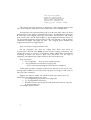
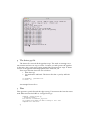
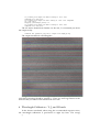
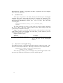
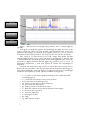
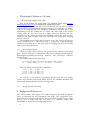
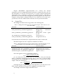
MOSFIRE SPECTROSCOPY DATA REDUCTION
PIPELINE:
USER MANUAL
Nicholas Konidaris March 7, 2014 1 Preface
This manual describes the installation of the MOSFIRE data reduction
pipeline on a unix-like computer. The pipeline has been tested on OSX and
Linux.
The MOSFIRE spectrograph data reduction pipeline was architected by
the MOSFIRE commissioning team and written by Nick Konidaris with
extensive checking and feedback from Chuck Steidel and other MOSFIRE
team members. The pipeline is maintained on an online code repository
mosfire.googlecode.com. Please use this website to track issues and and submit
requests.
To post comments please send an email to (you do not need to “join” the
group or have a Google email account):
[email protected]
2 Installing the Data Reduction Pipeline
1. The pipeline relies on the Ureka Python distribution produced by STScI and
Gemini Observatory. Follow the instructions at this link:
http://ssb.stsci.edu/ureka/1.0
2. Download the MOSFIRE DRP from mosfire.googlecode.com. This
command will create the ~/mospy command, which is a wrapper around
python.
cd ~
wget http://www.astro.caltech.edu/~npk/mosdrp_releases/mosdrp_cur.tgz
mkdir mosdrp
cd mosdrp
tar -xzf ~/mosdrp_cur.tgz
cp apps/mospy ~/mospy
chmod +x ~/mospy
Edit ~/mospy and update MOSPATH to the path ~/mospy, expand out the
twidle to the full path name. For instance, on my computer at Caltech I’ve
copied the data reduction pipeline to /scr2/mosfire/DRP/mosfire
1
The installation has now:
• Installed the data reduction pipeline to ~/mosdrp including:
o The bad pixel mask to ~/mosdrp/badpixels
o The data reduction pipeline code to ~/mosdrp/MOSFIRE
o Mospy applications including:
§ what – useful pretty printer for files
§ handle – the entry point for creating driver files (more
later)
o Example “Driver” files ~/mosdrp/Driver.py and one for the K
band in ~/mosdrp/K_driver.py
• Created an executable shell script called mospy in ~/
From now on, if you want to run any pipeline commands, you will always
execute
~/mospy
Did you use a previous version of the pipeline? If so, you will notice that the
concept of a default input/output directory is now gone. You also don’t need
to install mercurial. Now that’s progress.
3 First Step: Handle
Note: This has changed compared to the stsci_python version of MOSDRP.
The pipeline needs to know what files you have. The handle step will
parses the FITS header information and determine what files are associated
with each of your masks. The step creates a set of directories organized as
[maskname]/[date]/[band]/
Aborted.txt: Aborted files
Align.txt: Alignment frames
Ar.txt: Argon spectra
Dark.txt: Darks
2
Flat.txt: Flat fields
Image.txt: Imaging mode
MIRA.txt: MIRA focus images
Ne.txt: Neon lamp spectra
Unknown.txt: Unknown files
Offset_[p].txt: Science frames
The output directory structure is designed to make finding reduced data
easy, and to seaprate reductions of the same mask across multiple dates.
You will then edit a provided driver file to reduce the data. There are three
provided driver files that are nominally located in ~/mosdrp/drivers: Driver.py,
K_Driver.py, and Longslit_Driver.py. The Driver and K_Driver will reduce
your science data. The K band requires a special approach because there are
too few bright night-sky emission lines at the red end and so the K_Driver
synthesizes arclamps and night sky lines. The Longslit_Driver handles the
longslit observations of single objects.
First, you need to setup your directories.
On my computer, the data are copied from Keck and stored in
/scr2/mosfire/. NOTE: You must preserve Keck’s naming convention. The
output directory I’ve chosen is /scr2/npk/m3. Please adjust these instructions
according to where you want to place your directories. For the sake of
simplicity, the pipeline will output results to the current directory.
Steps to perform
1. cd /scr2/npk/m3
# Go to your output directory
2. ~/mospy handle /scr2/mosfire/2013sep24/*fits
… A lot of data summarizing the observations is outputed
At this point you have a number of directories and files. If you see an error
message like “Couldn't IO /scr2/mosfire/2013sep24/” you forgot to add a *fits at
the end of the command.
Suppose you want to reduce the data from mask Q0105msfr2.ws in H
band? Now you simply perform two steps:
1. cd /scr2/npk/m3/Q0105msfr2.ws/2013sep24/H
2. cp ~/mosdrp/drivers/Driver.py .
3. NOTE: If you are observing a K band mask you’ll want to copy the
K_driver.py file over.
An example output follows:
3
4 The driver.py file
The driver file controls all the pipeline steps. The trick to running it is to
uncomment and run one step at a time. I assume you will operate the pipeline
in this way. Also, some steps require output files from previous steps. A future
version of the pipeline will autopopulate these fields for you.
First steps with the driver file are as follows:
1. Edit driver.py
2. Set maskname and band. The driver files line 14 and 15 will look
like:
14 maskname = 'Q0105msfr2.ws'
15 band = 'H'
An example Driver file is
5 Flats
Flats generate a pixel flat and slit edge tracing. Uncomment the line that starts
with #Flat and run the DRP as ~/mospy Driver.py:
ramekin% ~/mospy Driver.py
… Truncated output …
Flat written to combflat_2d_H.fits
00] Finding Slit Edges for BX113 ending at 1901. Slit
composed of 3 CSU slits
4
01] Finding Slit Edges for BX129 ending at 1812. Slit
composed of 2 CSU slits
02] Finding Slit Edges for xS15 ending at 1768. Slit composed
of 1 CSU slits
Skipping (wavelength pixel): 10
03] Finding Slit Edges for BX131 ending at 1680. Slit
composed of 2 CSU slits
The slit names should look familiar. At the end, I recommend you check
the output in ds9:
ramekin% ds9 pixelflat_2d_H.fits -region slit-edges_H.reg
The output should look something like:
The green lines must trace the edge of the slit. If they don’t, then the flat
step failed. All values should be around 1.0. There are some big features in the
detector that you will become familiar with over time.
6 Wavelength Calibration – Y, J, and H bands:
In the shorter wavebands, when using the recommended exposure times,
the wavelength calibration is performed on night sky lines. The mospy
5
Wavelength module is responsbile for these operations. See the example
driver file in the appendix.
6.1
Combine files
First step is to produce a file with which you will train your wavelength
solution. Since we’re using night sky lines for training, the approach is to
combine individual science exposures. This is performed by the python
Wavelength.imcombine routine. For a lot of users, this will look
something like:
Wavelength.imcombine(‘Offset_1.5.txt’, maskname, band,
options)
The first parameter is ‘Offset_1.5.txt’ which is a python string indicating
the list of files in the first offset position. Note that Offset_1.5.txt was
generated by the handle command.
Suppose you want to exclude a file for reasons such as weather or telescope
fault, simply remove the offending file from Offset_1.5.txt. Likewise, you are
welcome to add files in as you like.
Outputs of this step are:
Filename
wave_stack_[band]_[range].fits
6.2
Contains
A median-combined image of the
files to be used for the wavelength
solution.
Interactive wavelength fitting
The DRP now needs to find the wavelength solution in the wave_stack_* file.
Here we interactively fit the lines. This step is interactive. The call looks like:
Wavelength.fit_lambda_interactively(maskname,band,
'Offset_1.5.txt', waveops)
This code uses ‘Offset_1.5.txt’ to load the wave_stack file generated in the
previous step. When you run this step, a GUI window appears:
6
Spectra
Residual
wavelength
Ignore
these buttons
Figure 1 – The interactive wavelength solving window. This is a J-band night sky
spectrum.
Your goal is to help the pipeline by identifying the night sky lines in the
center of each slit. Once you come up with a good solution in the center, the
pipeline will propagate it outwards. The pipeline uses Press ? to see a list of
commands in the console window. The steps you need to take are as follows.
First, zoom in (‘z’) and check to see if the orange lines match up with
obvious night sky lines. If not, move the plots by pressing the ‘c’ button. The
‘c’ button shifts the measured spectrum in the wavelength direction. Once the
spectrum is aligned with the known night sky positions press ‘f’ to fit. A
Chebyshev polynomial, f, such that f(pixel #) returns the wavelength in
Angstrom.
Continue this until you see the red Done! text in the center of your screen.
Plotted in the gui will be a sky line spectrum and vertical lines denoting positions and wavelengths of the sky lines. You will interactively fit a wavelength
solution to the sky line spectrum. Options available on the gui are:
•
•
•
•
•
•
•
•
•
•
•
•
7
c - to center on the nearest peak (first thing to do to shift the initial
wavelength guess)
c - Center the nearest line at the cursor position
f - Fit the data (second thing to try)
d - Delete a point (remove the wackadoos)
n - proceed to the Next object
p - return to back to the Previous object
r - Reset the current slit (try this if the plot looks strange)
z - Zoom at cursor position
x - Unzoom: full screen
s - Save figure to disk
h - Help
q - Quit and save results
7 Wavelength Calibration – K band:
7.1
K-band only: merge neon + sky
Note: At the moment, the Argon lamp is not supported, please email [email protected] if you would like to contribute this feature.
The night sky lines at the red end of the K-band are too faint to achieve
small-fraction of a pixel RMS wavelength calibration. You will have to observe
a Neon arc lamp during your afternoon calibrations. Because the beams
emminating from the arclamp do not follow the same path as the beams
coming from the sky, there will be a slight difference between the two
solutions. For the afformentioned beam matching reason, the most accurate
solution is the night sky lines. Thus, the code has to be clever about merging
the two solutions.
The merging process takes places in three steps. The step is the same as
those described in S6.2. The second step is to generate a full wavelength
solution as described above. The final step is a merging step. The second and
final steps are described below.
7.1.1
Neon lamp solution
The neon lamp solution will use the generated sky solution as an initial
guess. You are welcome to interactively solve the neon lamp solution with the
Wavelength.fit_lambda_interactively; however, this interactive solutions
should be rare.
Uncomment the line in Driver-K.py:
33 Wavelength.apply_interactive(maskname, band, waveops,
34
apply='Offset_1.5.txt', to='Ne.txt', neon=True)
This step, when run will produce output like:
slitno
slitno
slitno
slitno
1
2
3
4
STD:
STD:
STD:
STD:
0.16
0.03
0.04
0.05
MAD:
MAD:
MAD:
MAD:
0.06
0.02
0.04
0.01
For each slit, a new solution is generated for the neon line. The output
mimics that described previously where STD is the standard deviation and
MAD is the median absolute deviation in angstroms.
7.1.2
Merge sky and neon lamp
8 Background Subtraction
This DRP assumes that targets are nodded along the slit with integration
times as described on the instrument web page. The integration times
described were selected such that the shot-noise in the region between night
lines is over 5x larger than the read noise of a 16-fowler sample. For
MOSFIRE, we define this as background limited.
8
Despite MOSFIRE’s (unprescedented) f/2.0 camera, the desired
integration time for background-limited operation is longer than the time for
the atmosphere to vary by several percent. As a result, a further background
subtraction step is required to remove the residual features. The step is
performed by a function called background_subtract_helper() and follows the
notation and procedure outlined in Kasen (2003; PASP 115). For most users,
you’ll want to use the standard Driver file and not worry about the details.
8.1
Output Files
The background subtraction step produces the following files.
Table 1 - Background subtraction step unrectified outputs. These files are used
later in the DRP.
Filename
sub_[maskname] _[bandname]_[plan].fits
bsub_[maskname]_{ bandname]_[plan].fits
bmod_[maskname]_{ bandname]_[plan].fits
std_[maskname]_{ bandname]_[plan].fits
itime_[maskname]_{ bandname]_[plan].fits
Content (units)
Signal (𝑒 ! /𝑠)
Background
subtracted
!
signal (𝑒 /𝑠)
Background model signal
(𝑒 ! /𝑠)
Total noise (𝑒 ! )
Integration time (𝑠)
As usual elements in [brackets] are replaced with the value for that mask.
Recitified outputs are also computed as tabulated in Table 2.
Table 2 - Background subtracted and rectified outputs. The following files are not
used in the later steps of the DRP, they are provided for convenience.
Filename
[maskname]_pair_[bandname]_[plan].fits
[maskname]_pair_itime_[bandname]_[plan].fits
[maskname]_pair_std_[bandname]_[plan].fits
[maskname]_pair_sn_[bandname]_[plan].fits
Content (units)
Signal (electron/second)
Integration time (second)
Standard deviation (electron)
Signal to noise ()
Note that signal to noise is computed as follows:
𝑠𝑖𝑔𝑛𝑎𝑙 ⋅ 𝑖𝑛𝑡𝑒𝑔𝑟𝑎𝑡𝑖𝑜𝑛 𝑡𝑖𝑚𝑒
𝑠𝑛 =
𝑠𝑡𝑑
yes, we violate the first normal form for convenience. Also note that the
STD is computed assuming the detector has a read noise of Detector.RN
(documented in the MOSFIRE Pre Ship Review as 21 electron) per fowler
sample. Thus, the final STD is
21 𝑒𝑙𝑒𝑐𝑡𝑟𝑜𝑛
𝑆𝑇𝐷 =
+ # 𝑑𝑒𝑡𝑒𝑐𝑡𝑒𝑑 𝑒𝑙𝑒𝑐𝑡𝑟𝑜𝑛
𝑁!"#$%
assuming the gain in Detector.gain. Note that there is no shot noise from
dark current, which was measured to be negligible at pre-ship review.
An example of what the output looks like is here:
9
9 Longslit Reductions
The longslit reductions require transferring the Longslit_Driver.py file into
the reduction directory. A few key parameters have to be adjusted in
Longslit_Driver.py to help the pipeline figure out where to extract the longslit
from.
1. cd /path/to/LONGSLIT/
2. cp ~/mosdrp/drivers/Driver_Longslit.py .
3. Check all the .txt files to make sure your observations are included.
You may have to merge files from various LONGSLIT*
directories. This happens when your observations use a shorter
longslit than the calibrations.
4. edit Driver_Longslit.py
a. Change band = ‘FILL’ to the band
b. Examine a longslit image (see figure below) and adjust
‘yrange’: [709, 1350] to the vertical range
c. From the same examined longslit, select ‘row_position’ so
that it is uncontaminated. See Figure 2.
d. The result should look like Figure 3.
5. Decide if you want to use Neon or sky lines for the wavelength
solution.
6. For each step in a section, uncomment the necessary line and run
mosdrp on the Driver file. Once the apply_lambda_simple step is
10
complete, fill in the ‘lambda_solution_wave_stack_...’ line with the
correct wave stack file.
You now have two options based on the results. If the night sky lines are
not bright enough to identify in the interactive step you should use arclamps.
In the following instructions, replace wavefiles with ‘Ne.txt’.
Figure 2- An example of an uncontaminated row (#1127) in the longslit.
11
Figure 3- Example of a modified Driver_Longslit.py. Notice that pixel 991 is
selected as the row to perform the initial wavelength solution on. In Figure 2, this is
the equivalent of 1127.
10 Some Hints
10.1 Pay attention to the wavelength fitting output:
12
The output above shows that up to pixel 1015 the RMS was 0.27 Angstrom
level, and then dramatically jumped to 60 angstrom. Look at the image and
examine pixel 1016, figure out what happened. You may have to adjust your
input files or remove a file from the set.
10.2 Look at rectified_wave_stack files
Look at rectified_wave_stack* files and make sure the night sky lines are
vertical on the detector.
13