1
NEMO5
User Manual
May 17, 2012
Author:
Sebastian Steiger
Lead:
Prof Gerhard Klimeck
NEMO5 core developers:
Michael Povolotskyi
Tillmann Kubis
Hong-Hyun Park
Sebastian Steiger
Network for Computational Nanotechnology
Purdue University
West Lafayette IN, USA
Contents
1 Introduction
1.1 The purpose of NEMO5 . . . . . . . . . . . . . .
1.2 Key elements that distinguish NEMO5 from other
1.3 Short history of NEMO5 . . . . . . . . . . . . . .
1.4 To whom this manual is addressed . . . . . . . .
1.5 License . . . . . . . . . . . . . . . . . . . . . . . .
1.6 Additional sources of information . . . . . . . . .
1.7 nanoHUB tools employing NEMO5 . . . . . . . .
.
.
.
.
.
.
.
3
3
4
4
5
5
6
6
2 Installation
2.1 Obtaining pre-compiled versions . . . . . . . . . . . . . . . . . . . . . . . . .
2.2 Installation from source . . . . . . . . . . . . . . . . . . . . . . . . . . . . .
2.3 Directories . . . . . . . . . . . . . . . . . . . . . . . . . . . . . . . . . . . . .
7
7
8
8
3 Input and Output
3.1 Input . . . . . . . . . . . . . . . . . . . . . .
3.1.1 The material file . . . . . . . . . . .
3.1.2 Specifying material parameters in the
3.2 Output . . . . . . . . . . . . . . . . . . . . .
3.2.1 Visualization tools . . . . . . . . . .
4 The Input Deck
4.1 Example . . . . . . . . . . . . .
4.2 Structure section . . . . . . .
4.2.1 Material sections . . . .
4.2.2 Geometry section . . . .
4.2.2.1 Region sections
.
.
.
.
.
.
.
.
.
.
.
.
.
.
.
1
.
.
.
.
.
.
.
.
.
.
.
.
.
.
.
.
.
.
.
.
. . . . . .
simulators
. . . . . .
. . . . . .
. . . . . .
. . . . . .
. . . . . .
. . . . . . .
. . . . . . .
input deck
. . . . . . .
. . . . . . .
.
.
.
.
.
.
.
.
.
.
.
.
.
.
.
.
.
.
.
.
.
.
.
.
.
.
.
.
.
.
.
.
.
.
.
.
.
.
.
.
.
.
.
.
.
.
.
.
.
.
.
.
.
.
.
.
.
.
.
.
.
.
.
.
.
.
.
.
.
.
.
.
.
.
.
.
.
.
.
.
.
.
.
.
.
.
.
.
.
.
.
.
.
.
.
.
.
.
.
.
.
.
.
.
.
.
.
.
.
.
.
.
.
.
.
.
.
.
.
.
.
.
.
.
.
.
.
.
.
.
.
.
.
.
.
.
.
.
.
.
.
.
.
.
.
.
.
.
.
.
.
.
.
.
.
.
.
.
.
.
.
.
.
.
.
.
.
.
.
.
.
.
.
.
.
.
.
.
.
.
.
.
.
.
.
.
.
.
.
.
.
.
.
.
.
.
9
9
9
10
10
11
.
.
.
.
.
12
12
16
16
19
19
Contents
4.3
4.4
CONTENTS
4.2.2.2 Boundary region
4.2.3 Domain sections . . . . . .
4.2.4 Partitioning section . .
Solvers section . . . . . . . . . .
Global section . . . . . . . . . .
sections
. . . . .
. . . . .
. . . . .
. . . . .
.
.
.
.
.
.
.
.
.
.
5 Solvers and Options
5.1 Options common to all solvers . . . . . . . . .
5.2 Structure . . . . . . . . . . . . . . . . . . . .
5.3 VFFStrain . . . . . . . . . . . . . . . . . . . .
5.4 Phonons . . . . . . . . . . . . . . . . . . . . .
5.5 NonlinearPoisson . . . . . . . . . . . . . . .
5.6 Poisson . . . . . . . . . . . . . . . . . . . . .
5.7 Schroedinger . . . . . . . . . . . . . . . . . .
5.8 Semiclassical . . . . . . . . . . . . . . . . .
5.9 WF . . . . . . . . . . . . . . . . . . . . . . . .
5.10 NEGF . . . . . . . . . . . . . . . . . . . . . . .
5.11 TopOfBarrier . . . . . . . . . . . . . . . . . .
5.12 Ramper . . . . . . . . . . . . . . . . . . . . . .
5.13 ResonanceFinder . . . . . . . . . . . . . . . .
5.14 Angel . . . . . . . . . . . . . . . . . . . . . .
5.15 MatrixElements . . . . . . . . . . . . . . . .
5.16 Brillouin . . . . . . . . . . . . . . . . . . . .
5.17 DriftDiffusion . . . . . . . . . . . . . . . .
5.18 Propagation . . . . . . . . . . . . . . . . . .
5.18.1 Greensolver (subtype of Propagation)
5.18.2 Self energy (subtype of Propagation)
5.19 SimulationModules . . . . . . . . . . . . . .
5.20 Contacts . . . . . . . . . . . . . . . . . . . .
6 Material Parameter Names
6.1 Structure, Brillouin . . .
6.2 VFFStrain, Phonons . . . .
6.3 Poisson, NonlinearPoisson
6.4 Schroedinger, WF, NEGF . .
6.5 Semiclassical . . . . . . .
Bibliography
NEMO5 User Manual
.
.
.
.
.
.
.
.
.
.
.
.
.
.
.
.
.
.
.
.
.
.
.
.
.
.
.
.
.
.
.
.
.
.
.
.
.
.
.
.
.
.
.
.
.
.
.
.
.
.
.
.
.
.
.
.
.
.
.
.
.
.
.
.
.
.
.
.
.
.
.
.
.
.
.
.
.
.
.
.
.
.
.
.
.
.
.
.
.
.
.
.
.
.
.
.
.
.
.
.
.
.
.
.
.
.
.
.
.
.
.
.
.
.
.
.
.
.
.
.
.
.
.
.
.
.
.
.
.
.
.
.
.
.
.
.
.
.
.
.
.
.
.
.
.
.
.
.
.
.
.
.
.
.
.
.
.
.
.
.
.
.
.
.
.
.
.
.
.
.
.
.
.
.
.
.
.
.
.
.
.
.
.
.
.
.
.
.
.
.
.
.
.
.
.
.
.
.
.
.
.
.
.
.
.
.
.
.
.
.
.
.
.
.
.
.
.
.
.
.
.
.
.
.
.
.
.
.
.
.
.
.
.
.
.
.
.
.
.
.
.
.
.
.
.
.
.
.
.
.
.
.
.
.
.
.
.
.
.
.
.
.
.
.
.
.
.
.
.
.
.
.
.
.
.
.
.
.
.
.
.
.
.
.
.
.
.
.
.
.
.
.
.
.
.
.
.
.
.
.
.
.
.
.
.
.
.
.
.
.
.
.
.
.
.
.
.
.
.
.
.
.
.
.
.
.
.
.
.
.
.
.
.
.
.
.
.
.
.
.
.
.
.
.
.
.
.
.
.
.
.
.
.
.
.
.
.
.
.
.
.
.
.
.
.
.
.
.
.
.
.
.
.
.
.
.
.
.
.
.
.
.
.
.
.
.
.
.
.
.
.
.
.
.
.
.
.
.
.
.
.
.
.
.
.
.
.
.
.
.
.
.
.
.
.
.
.
.
.
.
.
.
.
.
.
.
.
.
.
.
.
.
.
.
.
.
.
.
.
.
.
.
.
.
.
.
.
.
.
.
.
.
.
.
.
.
.
.
.
.
.
.
.
.
.
.
.
.
.
.
.
.
.
.
.
.
.
.
.
.
.
.
.
.
.
.
.
.
.
.
.
.
.
.
.
.
.
.
.
.
.
.
.
.
.
.
.
.
.
.
.
.
.
.
.
.
.
.
.
.
.
.
.
.
.
.
.
.
.
.
.
.
.
.
.
.
.
.
.
.
.
.
.
.
.
.
.
.
.
.
.
.
.
.
.
.
.
.
.
.
.
.
.
.
.
.
.
19
19
22
23
23
.
.
.
.
.
.
.
.
.
.
.
.
.
.
.
.
.
.
.
.
.
.
25
25
26
26
28
30
33
33
39
39
43
43
45
46
48
48
49
50
50
51
51
52
52
.
.
.
.
.
54
54
55
55
56
57
58
2
Chapter
1
Introduction
1.1
The purpose of NEMO5
NEMO5 [1] is intended to be an all-purpose nanoelectronics simulation toolbox. Its modular
design permits developers to add and extend physical models using clean APIs. Currently
NEMO5 is able to do the following:
• Construct atomistic representations of nanostructure using various elements, crystal
structures, crystal directions.
• Calculate the Brillouin zone of the corresponding reciprocal lattice.
• Calculate the relaxed atomic positions using various flavors of the valence force field
(VFF) model.
• Calculate phonon spectra using VFF models.
• Solve the atomistic tight-binding Schrödinger equation.
• Solve the Poisson equation and coupled Schrödinger -Poisson problems.
• Use the full-band eigenstates as input to a Top-Of-Barrier model for ballistic transport
in nanotransistors.
• Calculate transport properties such as current, transmission spectra, through the openboundary wave function formalism.
• Calculate transport properties such as current, transmission spectra, through the NEGF
formalism.
• There are also first attempts on phonon transport.
3
1.2. Key elements that distinguish NEMO5 from other simulators
CHAPTER 1. INTRODUCTION
1.2
Key elements that distinguish NEMO5 from other
simulators
• Advanced atomistic nanostructures of non-standard (i.e., non-zincblende) structures
can be constructed using primitive unit cells. Currently implemented are simple-cubic,
diamond, zincblende, wurtzite, and rhombohedral lattices.
• NEMO5 is highly MPI-parallelized, making it suitable for large-scale computations on
supercomputers.
• The code is written in a modular way with clear and well-documented interfaces. This
permits extensive testing of individual components, allows of code extensions and usage
of selected modules in other codes.
• The power of advanced numerical packages is leveraged: libmesh (for the FEM discretization of the Poisson equation), PETSc (for matrices, linear and nonlinear equation systems), SLEPc (for eigenvalue problems), qhull (for the Voronoi cell), boost (for
parsing the input deck and a few filesystem operations), VTK (as an output format),
Silo (as a parallel output format) and others.
1.3
Short history of NEMO5
NEMO5 was started by the 4 post-docs (in alphabetical order) Tillmann Kubis, Hong-Hyun
Park, Michael Povolotskyi and Sebastian Steiger in the group of Prof Gerhard Klimeck at
Purdue University. It draws upon extensive prior experience of the group in nanoelectronics
simulation:
• NEMO-1D [2] was historically the first simulation tool to correctly predict I-V curves
of resonant tunneling diodes (RTDs), which is a prototypical nanoelectronic device. It
was a large and successful project being co-led by Gerhard Klimeck in the mid-90s and
featured tight-binding Schoedinger-Poisson and NEGF functionality.
• NEMO-3D [3,4] focused on atomistic Schroedinger-Poisson simulations of large systems
(such as quantum dots consisting out of millions of atoms). It was developed in the early
2000s under Gerhard Klimeck’s supervision at JPL. It includes calculations of strain,
polarization and optical matrix elements and is still being used. Its main achievement
was the ability to carry out massively parallel calculations employing 1000’s of CPUs
at the same time.
• OMEN [5] is the work of Mathieu Luisier and has been developed from 2005-2010
at ETH Zurich and Purdue. It is able to accurately compute transport in nanowires,
HEMTs, MOSFETs, TFETs and other devices in a massivey parallel way (near-perfect
scaling up to 200’000 cores was demonstrated).
NEMO5 User Manual
4
1.4. To whom this manual is addressed
CHAPTER 1. INTRODUCTION
• NEMO-3D [?] has been extended from 2008-2010 by Sunhee Lee and Hoon Ryu to
have a 3D space parallelization, Coulomb and exchange matrix element calculations,
and more. Its main target has been the massively parallel computation of properties
of phosphorus impurities in Si.
Given these four prior incarnations of NEMO (NanoElectronics MOdeling), the authors decided to call their tool NEMO5.
In addition to the knowledge of the group, the experience of the authors from their prior
jobs was pivotal in the development of NEMO5. Each was involved in large-scale projects,
amongst which are NextNano, TiberCAD, tdkp/AQUA, Simsn, and other projects.
1.4
To whom this manual is addressed
This manual might be beneficial to the following classes of people:
• Researchers in the nanoelectronics area who are in need of a simulation and want to
know if NEMO5 can help them.
• NEMO5 Users who want to understand the full functionality of NEMO5 and how to
set up input decks and correct simulation parameters.
• NEMO5 Developers who are unclear about the meaning of certain classes or keywords. However, most of the documentation relevant to developers is provided through
doxygen in the source code.
What you will find in this manual, and what you don’t
This manual should provide the user with an accurate and complete description on the
functionality of NEMO5 and on how to run simulations, i.e. setting up an input deck and
obtaining results. However, it cannot explain all the output generated by the simulator, or all
the possible error messages. It can also not explain the entire physics behind the simulation:
if the reader does not know what the Schrödinger equation is of what the local density of
states in NEGF means, then he or she has to consult other sources of information.
1.5
License
NEMO5 is distributed under the NEMO5 academic license. This means that it is free for
academic use. Commercial use is not permitted under this license and requires a different
license.
NEMO5 User Manual
5
1.6. Additional sources of information
1.6
CHAPTER 1. INTRODUCTION
Additional sources of information
In case the reader is in need of additional information, he may think about doing one of the
following:
• Check the developer documentation that is provided with the source code in the doc/
folder.
• Supplementary material (such as Powerpoint slides) is available in the supplements/
folder.
• A scientific paper has been published [1].
• Send Gerhard Klimeck, one of his group members or one of the developers an e-mail.
1.7
nanoHUB tools employing NEMO5
NEMO5 is the engine of the following tools on nanoHUB.org:
• Quantum Dot Lab:
https://nanohub.org/tools/qdot
• 1D Heterostructure Tool:
https://nanohub.org/tools/1dhetero
• Crystal Viewer:
https://nanohub.org/tools/crystal viewer
• Brillouin Zone Viewer:
https://nanohub.org/tools/brillouin
These tool mainly consist of Rappture GUIs and translating wrappers that create input decks
for certain use cases out of user-supplied options and retrieve simulation output.
Incorporation of the following tools is in progress:
• Band Structure Lab:
https://nanohub.org/tools/bandstrlab
• Resonant Tunneling Diode Simulation with NEGF:
https://nanohub.org/tools/rtdnegf
NEMO5 User Manual
6
Chapter
2
Installation
2.1
Obtaining pre-compiled versions
Ready-to-use versions can be downloaded from nanoHUB:
https://nanohub.org/groups/nemo5distribution
Currently only Linux operating systems are supported. The following platforms are available:
• Kubuntu 10.04 64bit using the GCC compiler.
• Red Hat (RHEL4) 64bit using GCC, as set up on coates.rcac.purdue.edu.
• Debian 2.6.24 (Lenny) 64bit, as set up on nanohub.org.
Installation of such a distribution is straightforward:
1. Download the archive (.tar.gz) and save in an appropriate location.
2. The command tar zxvf <file>.tar.gz will extract NEMO 5.
3. A quick check whether it works can be done by running NEMO 5 on the supplied
.in-file.
The distribution may require some packages which are not installed by default, such as boost,
the GCC compiler, and so on. However, all these packages are free and easy to obtain.
7
2.2. Installation from source
2.2
CHAPTER 2. INSTALLATION
Installation from source
NEMO 5 has a fairly automated build system, however, problems can arise from the large
number of required 3rd-party libraries which need to be present for the configuration. The
user may follow these steps:
1. Download the source code archive from
https://nanohub.org/groups/nemo5distribution
and save in an appropriate location.
2. Extract the archive.
3. Follow the instructions in the provided README file.
2.3
Directories
NEMO 5 has the following directories:
Location of executable (binary) nemo.
Various software projects that use a part of NEMO 5 (e.g. the input
parser or the MPI parallelization scheme) as a library. These projects
are not considered to be part of NEMO 5.
doc/
doxygen developer documentation.
examples/
Example input decks that can be used as templates.
include/
C++ header files that can be used for the development of other codes
when using NEMO 5 as a library.
lib/
The shared NEMO 5 libraries.
manual/
This user manual.
materials/ Material parameters. Currently all parameters are condensed in a single
file all.mat.
src/
The source code. Users should not have to look at this directory.
supplement/ Loose pieces of additional information about implementation approaches,
physical models, etc.
tests/
A suite of tests to test the functionality of individual modules.
bin/
contrib/
NEMO5 User Manual
8
Chapter
3
Input and Output
3.1
Input
The simulation is steered through a single file, the input deck, which is described in detail in
chapter 4. A second type of input are the material parameters.
3.1.1
The material file
Currently all material parameters are provided through a single file. The user is free to
use his/her own file through specification in the input deck, but the NEMO distribution
comes with the file materials/all.mat. Inspection of the file reveals that it is more than a
mere collection of numbers. NEMO parses and understands simple mathematical expressions
entered for a parameter, something that comes in handy when e.g. a temperature dependence
of the lattice constant or the band gap shall be included. A few simple rules govern the syntax
of the file:
• Parameters are grouped and hierarchized using the group keyword. The top group
specifies the material.
• Entries must have an end of line character ;. Omission of ; has the result that the
next entry will not be recognized.
• Possible mathematical operators include +, -, *, /, ^, sqrt as well as round brackets
().
• Parameters can be cross-referenced, but a parameter that is not in the same (sub)group must be preceded with its full location with groups separated by a colon. Example: GaAs:Lattice:a lattice.
9
3.2. Output
CHAPTER 3. INPUT AND OUTPUT
• Double quotation marks (") should be used for strings.
• If the code requests a numerical entry for some parameter, NEMO will try to parse
whatever expression is given and throw an error if the result is not convertable into a
number.
• The code is smart in that entries are only evaluated when they are requested. This
means that a parameter can be reset and all parameters depending on it will have the
modified value when they are being read the next time. This should however not be
relevant to the user since it is up to the code to handle these things correctly.
The material database is a stand-alone module and was originally developed by Ben Hailey
at Purdue.
3.1.2
Specifying material parameters in the input deck
In addition to modifying material file, a user is able to specify material parameters in the
input deck. Such a specification will supercede whatever entry is present in the material file,
however if other parameters in that file depend on the specified parameter, an update of
these parameters is not automatic. There are some cases where NEMO does these updates
by an additional call to the material database, but the user should be cautious and check
that the correct parameters are used.
An input deck material parameter is placed in the corresponding Material section and needs
to have the full tree except for the material name, e.g. Lattice:a lattice.
3.2
Output
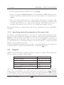
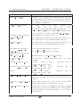
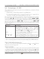
Output is provided in various formats depending on the type of output. The following table
gives an overview of possible output formats:
Data type
Atomistic structure
Atom-based fields
Continuum (i.e. non-atomistic) meshes
Vertex- or element-based continuum data
1-D (XY) data
File format
VTK, XYZ, PDB, Silo⋆
VTK, Silo⋆
VTK, PLT
VTK
ASCII
⋆
Silo is the only format that can be employed in simulations where the atomic grid is distributed onto several MPI processes. The atomic grid is saved in the form of a DB POINTMESH,
i.e. without the bonds, to reduce the file size and be able and generate molecule-type plots
in Visit. Atom-based data is saved as Ucdvar using the Multimesh and Poor Man’s Parallel
NEMO5 User Manual
10
3.2. Output
CHAPTER 3. INPUT AND OUTPUT
IO (PMPIO) concepts for parallel simulations. Currently there is only a single output file
containing the data aggregated from all processes that store the distributed grid.
VTK also comprises different internal formats. Atomistic data is saved in the POLYDATA format, the structure consisting of POINTS, VERTICES and LINES (this permits a visualization
as a molecule plot in Visit) and datasets being POINT DATA fields. Continuum data is saved
in the UNSTRUCTURED format, the mesh consisting of POINTS and CELLS.
The DX file format is implemented for the special case of fields on simple-cubic atomic lattices.
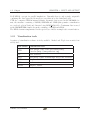
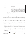
3.2.1
Visualization tools
A variety of visualization software is freely available. Matlab and Tecplot are non-free but
widely used.
File format Visualization tool
Visit (https://wci.llnl.gov/codes/visit)
VTK
Paraview (http://www.paraview.org)
Silo
Visit, Paraview
XYZ
Jmol (http://jmol.sourceforge.net), Visit, Paraview
PLT
Tecplot
PDB
Jmol
ASCII
Xmgrace, Matlab
NEMO5 User Manual
11
Chapter
4
The Input Deck
4.1
Example
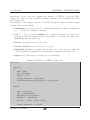
Listing 4.1 gives an example of an input deck. The example sets up a GaAs cube consisting
of 5x5x5 regular unit cells. The structure is first saved to a VTK file. Then a calculation
of a couple of quantum states in the sp3 s∗ d5 tight-binding model is performed using closed,
non-periodic boundary conditions, and the results are saved to file (atomic wavefunctions
again in VTK format). Lastly, overlap matrix elements between wavefunctions are computed
and saved to file. Although the various sections are discussed in detail in the later parts of
this chapter, a brief orientation is given here:
• The first section Structure contains information about structure and materials. Information about materials, its atomic composition, and nonstandard material parameters (i.e. additional or superceding the material parameter file) is contained in the
Materials subsection. The Geometry subsection specifies the geometric shape of individual regions. Currently a structure needs to be composed in the input deck and
cannot be read in from an external file. Lastly, the Domain subsections define which
regions are aggregated to a domain (each Simulation takes place on a certain Domain,
and there can be several Simulations carried out, possibly in a coupled way, using a
single input deck – such as in the present example).
• The section Solvers sets the Simulation types. Each simulation, given in a solver
subsection, has a set of options specific to its task.
• The section Global defines the location of the material parameters and which of the
defined Simulation entities are executed one after the other on the top level.
In the present input deck, there is only a single material type – GaAs –, a single region –
a cuboid – and a single domain that is being employed by all simulations. There are three
12
4.1. Example
CHAPTER 4. THE INPUT DECK
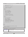
Simulation objects - one for the output of the domain to a VTK file, one for the Schrödinger solver, and one for the calculation of matrix elements between eigenfunctions of the
Schrödinger solver.
The remainder of the chapter is devoted to a detailed descriptions of these sections and their
options. Some general remarks:
• Comments are done in C++-style: // marks the remainder of a line as comment and
/* ... */ allows for multi-line comments.
• Only { ... } are accepted as brackets. The opening bracket needs to be put on the
same line as the section name and the closing bracket on a separate line. There is no
end of line character (such as ;).
• Vectors are given as (a,b,c) or (1,2,3).
• Vectors of vectors are given as [(a,b), (c,d)].
• Misspelled parameters are simply ignored and do not create an error, unless the
corrected parameter is mandatory in a simulation and missing in the input deck.
• Spaces can be either spaces or tabstops, it does not matter.
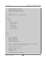
Listing 4.1: Example of a NEMO 5 input deck.
Structure
{
Material
{
name = GaAs
tag = substrate
regions = (1)
crystal_structure = zincblende
Bands:TB:sp3d5sstar_SO:param_set = param_Jancu
}
Domain
{
name = structure1
type = pseudomorphic
base_material = substrate
dimension = (20,20,20)
periodic = (false, false, false)
crystal_direction1 = (1,0,0)
NEMO5 User Manual
13
4.1. Example
CHAPTER 4. THE INPUT DECK
crystal_direction2 = (0,1,0)
crystal_direction3 = (0,0,1)
space_orientation_dir1 = (1,0,0)
space_orientation_dir2 = (0,1,0)
regions = (1)
geometry_description = simple_shapes
}
Geometry
{
Region
{
shape = cuboid
region_number = 1
priority = 1
min = (0,0,0)
max = (5,5,5)
tag = quantumdot
}
}
}
Solvers
{
solver
{
name = my_schroedi
type = Schroedinger
domain = structure1
active_regions = (1)
tb_basis = sp3d5sstar_SO
job_list = (assemble_H, passivate_H, calculate_band_structure)
output = (energies, eigenfunctions_VTK)
charge_model = electron_hole
automatic_threshold = true
chem_pot = 0.0
temperature = 300
eigen_values_solver = krylovschur
NEMO5 User Manual
14
4.1. Example
CHAPTER 4. THE INPUT DECK
number_of_eigenvalues = 10
shift = 0.5
k_space_basis = cartesian
k_points = [(0,0,0)]
}
solver
{
name = my_overlap
type = MatrixElements
domain = structure1
active_regions = (1)
operator = overlap
wf_simulation = my_schroedi
output_file = matrix_elements
}
solver
{
name = my_structure
type = Structure
domain = structure1
active_atoms_only = true
structure_file = structure.vtk
unit_cell_file = unit_cell.vtk
output_format = vtk
}
}
Global
{
solve = (my_structure,my_schroedi,my_overlap)
database = all.mat
}
The following color code will be used henceforth:
blue parameter Mandatory in all cases.
black parameter Optional (defaults will be used otherwise) or mandatory only in
some cases.
NEMO5 User Manual
15
4.2. Structure section
4.2
4.2.1
CHAPTER 4. THE INPUT DECK
Structure section
Material sections
Each appearing physical material – Si, GaAs and so on – must be described by such a
Material section. The aim of the section is to provide information about the crystallographic
structure (this information is necessary as e.g. nitrides may appear both in zincblende and
wurtzite phases) as well as material parameters that are not present in the parameter file or
should be overwritten.
Currently the following crystals are supported:
• diamond: FCC Bravais lattice with 2-atomic basis, where the 2 atoms have the same
type. Atoms at (0, 0, 0) and a/4(1, 1, 1). Lattice constant given by the parameter
Lattice:a lattice.
• zincblende: FCC Bravais lattice with 2-atomic basis, where the 2 atoms have different
type (cation and anion). Atoms at (0, 0, 0) and a/4(1, 1, 1). Lattice constant given by
the parameter Lattice:a lattice.
• simplecubic: Simple-cubic Bravais lattice with 1-atomic basis. Atom at (0, 0, 0).
Lattice constant (discretization) given by the parameter Lattice:a lattice.
• wurtzite: Hexagonal Bravais lattice with 4-atomic basis. Lattice constants given by
the parameters Lattice:a wurtzite, Lattice:c wurtzite and, for the determination
of the internal structure parameter u, Lattice:a lattice.
• hexagonal: Hexagonal Bravais lattice with 1-atomic basis. Lattice constants given by
the parameters Lattice:a wurtzite and Lattice:c wurtzite.
• Bi2Te3: Rhombohedral (trigonal) Bravais lattice with 5-atomic basis. All atoms
are on the z-axis. Lattice constants given by the parameters Lattice:a lattice,
Lattice:c lattice, Lattice:u lattice and Lattice:v lattice.
• graphene: Hexagonal Bravais lattice with 2-atomic basis. The third direction (c-axis,
[0001] direction) is meaningless. Lattice constants given by Lattice:a lattice.
• CNT: 1D-translational carbon nanotubes with a basis that depends on the user’s choice
of nanotube indices. By default the nanotube will be extended along the x-direction.
The lattice constant of the unrolled sheet is given by Lattice:a lattice.
• buckyball: C60 molecule, really only for the fun of it. Lattice constant given by
Lattice:a lattice.
• bcc: BCC Bravais lattice with 1-atomic basis. Atom at (0, 0, 0). Lattice constant given
by Lattice:a lattice.
NEMO5 User Manual
16
4.2. Structure section
CHAPTER 4. THE INPUT DECK
• caesiumchloride: Simple-cubic Bravais lattice with 2-atomic basis where the atoms
have different types. Atoms at (0, 0, 0) and a/2(1, 1, 1). Lattice positions are the
same as for BCC, but the atomic types are different. Lattice constant given by
Lattice:a lattice.
• sodiumchloride (rocksalt, NaCl): FCC Bravais lattice with 2-atomic basis where the
atoms have different type. Atoms at (0, 0, 0) and a/2(1, 0, 0). Lattice constant given
by Lattice:a lattice.
• tetragonal Tetragonal primitive (P ) Bravais lattice with 1-atomic basis. Lattice constants given by Lattice:a lattice and Lattice:c lattice.
• tetragonalI Tetragonal body-centered (I) Bravais lattice with 1-atomic basis. Lattice
constants given by Lattice:a lattice and Lattice:c lattice.
• orthorhombic Orthorhombic primitive (P ) Bravais lattice with 1-atomic basis. Lattice
constants given by Lattice:a lattice, Lattice:b lattice and Lattice:c lattice.
• orthorhombicC Orthorhombic base-centered (C) Bravais lattice with 1-atomic basis.
Lattice constants given by Lattice:a lattice, Lattice:b lattice and Lattice:c lattice.
• orthorhombicF Orthorhombic face-centered (F ) Bravais lattice with 1-atomic basis.
Lattice constants given by Lattice:a lattice, Lattice:b lattice and Lattice:c lattice.
• orthorhombicI Orthorhombic body-centered (I) Bravais lattice with 1-atomic basis.
Lattice constants given by Lattice:a lattice, Lattice:b lattice and Lattice:c lattice.
• monoclinic Monoclinic primitive (P ) Bravais lattice with 1-atomic basis. Lattice
constants given by Lattice:a lattice, Lattice:b lattice, Lattice:c lattice and
Lattice:alpha lattice.
• monoclinicC Monoclinic base-centered (C) Bravais lattice with 1-atomic basis. Lattice
constants given by Lattice:a lattice, Lattice:b lattice, Lattice:c lattice and
Lattice:alpha lattice.
• triclinic Triclinic Bravais lattice with 1-atomic basis. Lattice constants given by
Lattice:a lattice, Lattice:b lattice, Lattice:c lattice, Lattice:alpha lattice,
Lattice:beta lattice and Lattice:gamma lattice.
Please note that for crystals with a 1-atomic base the name of that atom is given by
Lattice:element (e.g., "Si") whereas for 2-atomic basis the atom names are given by
Lattice:cation and Lattice:anion.
Parameter
name
NEMO5 User Manual
Description
Material name
17
4.2. Structure section
CHAPTER 4. THE INPUT DECK
Parameter
tag
regions
Description
Additional description
A list of integers defining the regions that have this material
(definition takes place in the Region sections)
crystal structure
Crystallographic structure: see text for choices.
nanotube indices
Relevant only for carbon nanotubes (CNTs). This determines
the type of nanotube.
doping type
One of N or P.
doping density
The doping density in cm−3 .
charge model
Can be electron core or electron hole. In the former option there are no holes, only electrons, an the bands are populated starting from the very bottom.
doping ionization model Can be full ionization (default) or thermal ionization.
doping temperature
Related to incomplete
ionization: population of doping level
F
ED with factor 1 + exp( EDkT−E
)
D
ionization energy
doping degeneracy
?
disorder type
polarization
strain simulation
−1
.
Related to incomplete
ionization: population of doping level
−1
F
ED with factor 1 + exp( EDkT−E
)
.
D
Related to incomplete
ionization: population of doping level
−1
F
ED with factor 1 + exp( EDkT−E
)
.
D
Additional material parameters which replace the ones from
the material file (see also section 3.1.2).
In the case totally random dopant atomistically random
doping will be generated. In all other cases, doping is treated
in the virtual crystal approximation (Jellium model).
This optional 3-vector specifies the spontaneous (pyroelectric)
polarization of the material.
This optional specification of a strain solver will have a Poisson simulation get the strain tensor at every atomic location
and compute the piezo-electric polarization.
The doping should be a region property rather than a material property, but it is in here
for the moment.
NEMO5 User Manual
18
4.2. Structure section
4.2.2
Geometry section
4.2.2.1
Region sections
CHAPTER 4. THE INPUT DECK
These sections define the basic geometrical shapes that constitute the simulated structure.
Each region has a unique material (and crystallographic structure) which is associated in the
Material section.
Parameter
shape
tag
region number
priority
min, max
Description
One out of cuboid, spheroid, pyramid, cylinder or dome.
Additional description
A unique integer number associated with the region.
If regions are overlapping, this integer number determines which region
’wins’. A higher number means higher priority (wins). In case of overlapping regions with equal priorities, the outcome is somewhat arbitrary
and depends on the order of construction in the code.
Vectors that define corner points of the shape. The precise meaning
depends on the type of shape:
cuboid - two opposite corners.
spheroid - two opposite corners or the enclosing cuboid.
pyramid - two opposite corners or the enclosing cuboid (?).
cylinder - two opposite corners or the enclosing cuboid (?). Or you can use radius(r),
The pyramid and the cylinder currently have their axis along z. Note that after the geometry construction a rigid rotation of the whole structure can be performed using the
space orientation options in the Domain section.
4.2.2.2
Boundary region sections
These sections determine the contacts and can be the same 3D geometrical entities (with
the same options) as in a Region section. They have no direct influence on the constructed
atomic grid but can be used as special entities in certain solvers.
4.2.3
Domain sections
A Domain is a collegion of Regions and defines the structure on which a Simulation is solved.
NEMO5 User Manual
19
4.2. Structure section
CHAPTER 4. THE INPUT DECK
Parameter Description
name
The name of the domain.
type
One of pseudomorphic, finite elements. pseudomorphic
means a dislocation-free atomistic grid, finite elements
currently uses the atomic unit cells as finite elements for a
continuum grid.
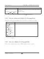
The remaining options depend on the type of domain.
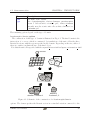
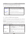
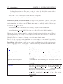
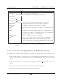
Pseudomorphic Domain options
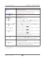
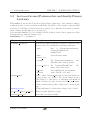
The construction of this type of domain is illustrated in Fig. 4.1. The final domain is the
intersection of a canvas, which is constructed by translations of the unit cell in the three
Bravais directions, with the regions specified in the domain. Depending on the size, either of
these two entities can limit the size of the final object.
Note that the unit cell is specified with the crystal directionN and space orientation dirN
unit cell
prio 1
prio
3
prio
2
canvas
regions
prio 1
prio
canvas
prio
3
2
●●●●●●
●●●●●●●●
●● ●●● ●●● ●
●●●●●●●●
●●●
domain 1 à solver 1
●●●
●● ●●
●●●
domain 2
à solvers 2, 3
Figure 4.1: Schematic of the construction of a PseudomorphicDomain.
options. The former specifies the Bravais vectors in a standard notation connected to the
NEMO5 User Manual
20
4.2. Structure section
CHAPTER 4. THE INPUT DECK
crystal. The latter provides the ability to perform a rotation of the constructed Bravais
vectors.
Parameter
regions
Description
A list of integer numbers describing the regions that constitute
the domain (as defined in the Region sections).
base material
Must correspond to a tag in one of the defined Material
entities.
dimension
This 3-vector gives the maximum extension, in unit cells,
that the domain has. It defines a parallelepiped from which
the regions will be cut out.
periodic
Entry X in this 3-vector defines whether the crystal is periodic in the direction crystal dimensionX. It can be true or
false.
crystal directionN
(N=1,2,3) These 3-vectors give the (cartesian) coordinates of
the vectors spanning the unit cell, in units of lattice constants.
crystal direction type plane or axis. Specified whether crystal directions define
crystal plane or crystal axis. Default is axis
space orientation dirN (N=1,2) These vectors determine a rotation of the whole crystal, such that e.g. the first unit cell vector can in the end be
pointing into the x-direction. The third vector is constructed
out of the first two.
geometry description
Can only be simple shapes at the moment. In the future this
parameter will determine whether the geometrical description
of the structure is given by Region and Boundary region
sections in the input deck, or whether it is read in from an
external file.
origin
A 3-vector that determines the starting point for the atomic
grid construction.
output
A list that currently can be either empty or contain xyz. This
option is deprecated since its functionality is replaced and
extended by the Structure simulation.
passivate
Putting false will deactivate the attachment of H-atoms at
non-periodic surfaces.
NEMO5 User Manual
21
4.2. Structure section
CHAPTER 4. THE INPUT DECK
Parameter
passivation regions
Description
This option matters for simulations where the tight-binding
Schrödinger equation is solved only on a subset of regions
(multiscale simulations). Atoms in regions with numbers contained in this list will be treated as Hydrogen-like in the tightbinding Schrödinger equation. Thus this list should be the
complement of the list given in the regions option of the
Schroedinger solver.
conformal partitioning
Putting false will enable broken unit cells at the structure
edges.
FEM 1D
A boolean that determines whether a 1D or a 3D FEMPoisson equation will be set up. Setting this option to true
speeds up 1D Schrödinger -Poisson simulations tremendously.
Table 4.2: PseudomorphicDomain parameters.
Note that for 2D-like graphene, 1D-like carbon nanotubes and 0D-like C60 buckyballs the
Bravais vectors are meaningless. They are arbitrarily chosen to have some large value.
Continuum Domain options
Currently the FEM mesh is created out of the unit cells of the atomistic domain.
mesh from domain The name of the atomistic domain from which the FEM mesh
is built.
4.2.4
Partitioning section
This optional section determines the distribution of the grid(s) onto multiple CPUs in the
case of MPI-parallelized simulations. Currently this distribution is done in a “3D-cuboid”
way. A user has two options:
1. The user specifies the minimum and maximum extension in each direction plus the number
of CPUs he/she wants for the distribution. In this case the options are:
{x,y,z} extension Three vectors with two entries (xmin,xmax) etc. that specify
the extension of the structure. All atoms must be contained
in the cuboid, and the cuboid should be fitted tightly to the
actual structure.
num geom CPUs
The number of MPI process to employ in the grid distribution.
When this parameter is omitted then the maximum number
is employed. Note that this number must be formable as a
product nx ny nz where nx,y,z ≥ 1.
NEMO5 User Manual
22
4.3. Solvers section
CHAPTER 4. THE INPUT DECK
The code will choose the combination (nx , ny , nz ) with a minimal surface between the partitions.
2. The user fine-tunes the partitioning by specifying the exact locations of the partition
interfaces.
{x,y,z} partition nodes Three lists with the location of the partition boundaries and
interfaces. The number of processes employed in the grid
distributed derived from nx ny nz , where the lists have nx,y,z +1
entries (nx,y,z ≥ 1).
4.3
Solvers section
This section consists of solver subsections. An example for an individual solver type would
be a Schroedinger calculator of electronic eigenstates and energies. These entities can, and
sometimes have to, interact with each other. A detailed description of all available solvers
including their parameters is provided in chapter 5.
4.4
Global section
This section contains global simulation options:
Parameter
solve
database
messaging level
logfile
output
Description
defines which of the defined Simulation types are actually solved. This
set will sometimes not be the same as given in the Solvers section. One
example could be a self-consistent Schroedinger-Poisson simulation, which
logically consists of three solver types – Schroedinger, Poisson and the
self-consistent coupler which utilizes the latter two – but only the solveroutine of the coupler is called. Why do it like this, you might ask? To
preserve the modularity of individual tasks: Imagine e.g. Schroedinger,
which really implements the atomistic tight-binding Hamiltonian, to be an
interchangeable module for the density calculation, replacable by a kp simulator, and so on.
the location of the material parameter file
A number between 0 and 6 that specifies the amount of terminal output. 0
is near-silent and 6 has a lot of debug output. Usually 2-4 is a good choice.
Levels 4-6 will invoke the memory managment reference counting output.
A file where terminal output gets saved into.
defines simulations that will perform output at the very end of NEMO5
execution.
NEMO5 User Manual
23
4.4. Global section
Parameter
petsc double report
petsc complex report
CHAPTER 4. THE INPUT DECK
Description
When set to true, then these options enable some terminal output at the
end of the simulation that provides statistics about double and complex
PETSc and SLEPc routines (SLEPc statistics are included in the PETSc
option). These statistics include peak memory, flops, and spent time per
PETSc/SLEPc routine and globally. The statistics do not include memory,
flops and time used outside PETSc/SLEPc.
NEMO5 User Manual
24
Chapter
5
Solvers and Options
This chapter describes the available solvers and their input deck parameters. A solver typically solves some set of equations, but there are also solvers which simply save something
to file or do simple post-processing. Therefore a more general name is Simulation. These
entities can interact and sometimes depend on other entities - the Poisson equation, which
solves for the electrostatic potential, needs to obtain the excess carrier charge from another
Simulation, for example. The color coding will be again as follows:
blue parameter Mandatory in all cases.
black parameter Optional (defaults will be used otherwise) or mandatory only in
some cases.
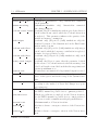
5.1
Options common to all solvers
Each solver (Simulation object) has the following common parameters:
Parameter Description
type
The simulation type: one of Structure, VFFStrain,
Phonons, Poisson, NonlinearPoisson, Schroedinger,
Semiclassical,
NEGF, WF, Propagation,
Ramper,
ResonanceFinder, MatrixElements, Angel or Brillouin.
name
A unique name tag / identifier for the specific instance of the
solver.
domain
The name of the domain on which the simulation is carried
out, corresponding the name parameter in the Domain section.
Table 5.1: Parameters common to all simulations.
25
5.3. VFFStrain
5.2
CHAPTER 5. SOLVERS AND OPTIONS
Structure (saving the structure to file)
This simulation outputs the atomistic structure of a certain domain to file.
Parameter
output format
Description
One of silo, vtk, jmol, pdb or (for simple cubic lattices
only) dx. If the structure is distributed onto several MPIprocesses (using the Partitioning section), only Silo is an
option.
structure file
The file into which the domain is saved.
info file
A file into which some crystallographic information is saved.
active atoms only (Default false) If true, then any non-active atoms (e.g. Hpassivation atoms connected to non-periodic surfaces) will not
be saved.
Table 5.2: Parameters of the Structure simulation.
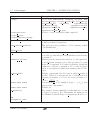
5.3
VFFStrain (VFF strain relaxation)
This simulation relaxes the atomic positions by minimizing the lattice energy computed via
the valence force field (VFF) model. Depsite the misleading simulation name, several models
for the energy functional are available through a mix-and-match approach steered by the
input deck.
Parallelism: The spatial parallelization given in the Partitioning section of the input deck
is employed to distribute the Hessian matrix as well as the displacement and right-hand-side
vectors onto multiple MPI processes. Like this a simulation of a 44-million InAs quantum
dot has been achieved using 216 CPUs.
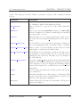
Parameter
models
num harmonic iters
anharm cutoff
NEMO5 User Manual
Description
A list that may contain the following: harmonic or
anharmonic Lazarenkova
or
anharmonic Areshkin
or anharmonic Sui;
stretch-bend;
cross-stretch;
coplanar-2ndNN; coulomb.
Taking the harmonic model while the Newton iteration is far
away from the solution improves convergence and speeds up
the simulation. This number specifies for how many iterations
this is done.
(anharmonic Lazarenkova only) dimensionless numerical
cutoff parameter.
26
5.3. VFFStrain
CHAPTER 5. SOLVERS AND OPTIONS
Parameter
anharm theta limit
Description
(anharmonic Lazarenkova only) dimensionless numerical
cutoff parameter.
anharm smoothing
(anharmonic Areshkin only) dimensionless numerical
smoothing parameter.
coulomb cutoff radius (coulomb only) For simulations without periodicity this is a
cutoff radius in nm outside which the Coulomb interaction
is neglected. This parameter influences the sparsity of the
matrix and memory consumption.
ewald sigma
(coulomb only) (3D-periodic (bulk) simulations only) the
standard deviation of the Gaussian used in the Ewald summation method, in nm.
coulomb ewald Kcut
(coulomb only) (3D-periodic (bulk) simulations only) integer
cutoff outside which the long-range contribution is neglected,
in units of reciprocal lattice vectors.
coulomb ewald Rcut
(coulomb only) (3D-periodic (bulk) simulations only) cutoff
in real-space
modify ideal length
(coulomb only) If set to true, then the parameter d which
in the absence of Coulomb interaction has the meaning of an
ideal bond length r0 is modified such that the enrgy functional
retains its minimum at r0 .
hessian info
If true then some numerical debug terminal output is created.
phonon solver
The name of the Phonons simulation object, if present. Existence of this option enables the set-up of the dynamical matrix.
calculate epsilon
If true then the strain tensor components are calculated
according to the method of Pryor and Zunger as a postprocessing step.
linear solver
Which linear solver is employed in the Newton iteration. See
the PETSc manual for possible choices - gmres is preferred.
preconditioner
Which preconditioner is employed in the Newton iteration.
See the PETSc manual for possible choices - asm is preferred.
lu does not work for simulations with grid-parallelization.
max num iters
Maximum number of Newton iterations.
absolute tol
Absolute tolerance convergence criterion of the Newton iteration.
relative tol
Relative tolerance convergence criterion of the Newton iteration.
NEMO5 User Manual
27
5.4. Phonons
CHAPTER 5. SOLVERS AND OPTIONS
Parameter
linsolver max iters
Description
Maximum number of linear solver iterations (in the case of an
iterative solver) for each Newton step.
linsolver monitor
If true then the convergence of the iterative linear solver is
monitored as terminal output.
vtk file
When set then the atomic displacement and possibly the
strain tensor are saved to a VTK file. Works only for simulations without grid parallelization.
vtk storage
Choose from ascii or binary.
silo file
When set then the atomic displacement and possibly the
strain tensor are saved to a Silo file.
test mat vec mult
Debug routine to test matrix-vector multiplication using the
Hessian of the strain simulation.
Table 5.3: Parameters of the VFFStrain simulation.
5.4
Phonons (phonon spectra)
In combination with the VFFStrain simulation this solver allows for the computation of
phonon spectra.
Parallelism: Since the phonon simulation uses the matrix that is constructed in VFFStrain
it has the same spatial parallelization, though this has not yet been tested. Additionally it
distributes the independent problems for each wavevector onto multiple MPI-processes. This
is done automatically.
Parameter
strain sim
output file
calculate sound
eta sound
calculate grueneisen
eta grueneisen
NEMO5 User Manual
Description
Name of the VFFStrain simulation object. That object sets
up the dynamical matrix.
Name of the file where to save the phonon dispersion.
If true then the speeds of sound are calculated as a postprocessing step.
Finite-difference parameter for the speed of sound computation.
If true then the Grüneisen mode parameters at Γ, X and L
are computed as a post-processing step.
Finite-difference parameter for the Grüneisen parameter computation.
28
5.4. Phonons
CHAPTER 5. SOLVERS AND OPTIONS
Parameter
calculate elastic
Description
If true then the bulk elastic constants are computed from the
VFF parameters.
calculate LO TO splitting
If true then the LO-TO splitting is computed.
eta LOTO
Optional parameter (in units 2π/a) to compute Γ-energies
slightly away from Γ during the LO-TO splitting computation.
bulk file
When set then all the above post-processing quantities are
saved into this file.
qspace basis
Sets in which basis the qpoints parameter is specified
(cartesian or reciprocal).
qpoints
A list of points in q-space along which the dispersion is calculated.
number of nodes
This list gives the uniform discretization of each segment set
by the qpoints parameter (note that specifying N points
means N − 1 segments).
shift wavevector to 1st BZ If true then every q-point is shifted back to the first BZ before
the computation.
eigensolver
Which eigensolver to take (choose from lapack, krylovschur,
arpack and others).
preconditioner
Optional choice of preconditioner. Default: lu.
num eigenvalues
Number of eigenvalues to compute (irrelevant for lapack since
all eigenvalues are computed there).
max num iters
Maximum number of Krylov iterations of the eigensolver.
convergence limit
Convergence limit below which an iterative eigensolver regards the value as converged.
monitor convergence
When set to true then the convergence of the Krylov iteration
is monitored in the terminal.
store polarization
True or false.
output polarization
Filename.
Table 5.4: Parameters of the Phonons simulation.
NEMO5 User Manual
29
5.5. NonlinearPoisson
5.5
CHAPTER 5. SOLVERS AND OPTIONS
NonlinearPoisson (Poisson solver and density-Poisson
iteration)
This simulation iterates the Poisson and Schrödinger equations to self-consistency using a
nonlinear predictor-corrector scheme in which the dependence of the density on the potential
is predicted. Like this a Newton iteration is carried out to find the electrostatic potential.
Such a scheme greatly improves convergence [6].
Note that this simulation object contains both the solution of the Poisson equation and the
Newton iteration with any density solver.
Parallelism: To be determined.
Parameter
boundary condition
Description
A subsection that specifies the boundary condition for the
Poisson solver. It contains the following parameters:
type
One of ElectrostaticContact,
PotentialFromSolver,
NormalField
name
Some arbitrary name.
boundary regions
For ElectrostaticContact:
the
Dirichlet value of the potential.
For PotentialFromSolver:
the
potential simulation
name of the other solver.
E field
For NormalField: the Neumann
D field
value of the E- or D- field.
Can be either electron hole (most cases), in which case
doping charges are added to the excess charges from a
Schroedinger or other solver, or electron core model in
which case there are only electrons and these are counterbalanced with a fixed positive charge based on the atomic
type.
A list with names of solvers where charge can be found.
Must be false (true has a bug)
Leave this one true (default).
voltage
charge model
density solver
use average density as a guess
average over cell
NEMO5 User Manual
30
5.5. NonlinearPoisson
Parameter
atomistic output
node potential output
one dim output
one dim output average
ksp type
pc type
linear solver maxit
max iterations
max nonlinear step
max function evals
rel tolerance
step abs tolerance
step rel tolerance
NEMO5 User Manual
CHAPTER 5. SOLVERS AND OPTIONS
Description
Save atom-based quantities to file.
The list can
contain the entries potential, charge, charge cm-3,
free charge, free charge cm-3, doping, doping cm-3,
conduction band and valence band. For simulations
without grid parallelization VTK is used as output format,
otherwise Silo.
If true, then the potential is written to (simname) nodal potential.dat.
Interpolates atom-based quantities onto an axis and generates 1D ASCII output compatible with 1D Matlabplots.
The list can contain the entries potential,
free charge cm-3, doping cm-3, conduction band and
valence band.
If true then unit cells are used for the 1D discretization
along some direction and some averaging is done within
the cells. If false then the orthogonal projection of the
atomic position serves as the 1D discretization.
Linear solver type. See the PETSc documentation for possible choices. Recommended are e.g. gmres or bcgs.
Preconditioner type.
See the PETSc documentation
for possible choices. Recommended are e.g. asm for
distributed-grid simulations, lu for small systems or
jacobi.
In case of an iterative linear solver, this is the maximum
number of iterations to solve the linear system.
Maximum number of Newton iterations (default: 100).
Not sure what the difference to the previous option is.
Maximum number of Newton right-hand-side evaluations
(default: 1000).
Relative residual tolerance of the Newton solver (default:
1e-6).
Absolute step tolerance of the Newton solver (default: 1e10).
Relative step tolerance of the Newton solver (default: 1e10).
31
5.5. NonlinearPoisson
Parameter
Newton solver only
set initial potential
constant intial potential
CB initial shift
VB initial shift
equilibrium el chem pot
do input initial
CHAPTER 5. SOLVERS AND OPTIONS
Description
If true, only a single step rather than the full selfconsistent iteration is performed. This option is typically
used when the Poisson solver is steered by another solver,
e.g. a transport simulation.
If
true,
then
some
initial
potential
will
be
either
read
in
from
file
(options
do input initial nonlinearpoisson potential
is
true) or computed (with an equilibrium Fermilevelwhich
is 0 by default or is given by equilibrium el chem pot).
Some number the potential can be set to.
If set, then the potential in n-type materials will be set to
the conduction band edge plus this number (in eV).
If set, then the potential in p-type materials will be set to
the valence band edge minus this number (in eV).
See set initial potential description.
See set initial potential description.
nonlinearpoisson potential
initial potential file name
set initial field
initial potential point
potential at initial point
field
do outputs from density solver
do nonlinearpoisson outputs xyz format
do output nonlinearpoisson potential
NEMO5 User Manual
Filename related to set initial potential.
If true, then a constant electric field will be set at the
beginning.
3-vector:
point in space.
Relevant only if
set initial field = true.
Potential at that point.
Relevant only if
set initial field = true.
Electric field (units??).
Relevant only if
set initial field = true.
If true, then the outputs specified in density quantum
solver can be obtained at the end of the NonlinearPoisson
solution.
If true, then output will be done in the cartesian XYZ
format, which is handy for Matlab-processing.
If true, then at the end of NonlinearPoisson, the potential
is output in a separate file in FEM format. This potential
can be used later to restart the simulation, or to do a fixed
potential run.
32
5.6. Poisson
CHAPTER 5. SOLVERS AND OPTIONS
Parameter
Description
initial potential file name
The name of the file containing the initial potential (see
previous option).
do output potential each iteration
When true, on each Schrodinger solve from NonlinearPoisson, the potential is output in a separate file in FEM format. This file is getting updated (overwritten) on each
such solve. This potential can be used later to restart the
simulation, or to do the fixed potential run. This is done if
convergence is not reached because of the crash or too long
run, the potential can still be obtained and simulation can
be restarted.
Table 5.5: Parameters of the NonlinearPoisson simulation (in addition to the Poisson parameters).
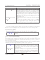
5.6
Poisson (linear Poisson solver)
This simulation solves the linear Poisson equation for a fixed density. Most options are the
same as for the NonlinearPoisson simulation, except for the obvious ones which are only
relevant in case of a nonlinear Newton-Raphson iteration.
5.7
Schroedinger (closed-boundary Schroediger solver)
This simulation solves the tight-binding Schrödinger equation. It calculates eigenenergies and
eigenstates as well as integrates the results to obtain electron and hole densities (if requested).
Band structure models: The band model is specified through the tb basis parameter.
Possible choices are the following:
• em: Effective mass in a current-conserving finite difference discretization due to Frensley (It can be also found in S. Datta’s book). The discretization also works for spatially vatying masses. Note that the crystal structure parameter must be set to
simplecubic.
• s: Effective mass in a fake tight-binding implementation. The obtained bulk band
structure is parabolic only in the vicinity of Γ. The discretization has problems with
inhomogeneous masses. Note that the crystal structure parameter must be set to
simplecubic.
• sp3sstar, sp3sstar SO, sp3d5sstar, sp3d5sstar SO: 5-, 10- and 20-band tight-binding
models. The suffix SO specifies whether the spin-orbit interaction is included or not,
NEMO5 User Manual
33
5.7. Schroedinger
CHAPTER 5. SOLVERS AND OPTIONS
doubling the system size. For purely electronic devices (no holes) the results without
spin-orbit interaction can sometimes be sufficiently accurate.
• Pz, P/D: 1- and 3-band tight binding models for graphene.
• ExtendedHuckel: ask M. Povolotskyi about this.
Influence of strain on band structure: In tight-binding the effect of strain on the band
structure is derived from the atomic positions. However, it is not sufficient to just do a
strain simulation, the influence on the Hamiltonian must be explicitly switched on through
the followin job list options:
• include strain H: Modifications according to Boykin’s 2002 formulation.
• include shear strain H: Modifications according to Boykin’s 2010 formulation.
When none of these options is included, a distorted crystal system will still produce a different
band structure due to the change of bond angles and hence modified direction cosines in the
tight-binding formula.
Currently there is no influence of strain on effective mass Hamiltonians.
Instead of doing a separate strain simulation one can superimpose a fixed strain by specifying
a matrix in the input deck (see table).
Parallelism: Schroedinger employes the spatial parallelism given in the Partitioning
section of the input deck. Additionally it distributes the k-points onto the different MPIprocesses. This is done automatically.
Parameter
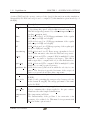
tb basis
use nonparabolic
epsilon matrix
epsilon matrix crystal
job list
NEMO5 User Manual
Description
The tight-binding basis / band structure model (see text).
(relevant only for choice tb basis=em) turn on nonparabolicity.
Constant strain tensor matrix, given in laboratory system coordinates. One needs to include strain in the job list in order
to use this.
Constant strain tensor matrix, given in crystal system coordinates. One needs to include strain in the job list in order
to use this.
A list that deterimes what is done. Choose from assemble H,
passivate H, include strain H, include shear strain H,
calculate band structure,
electron density,
derivative electron density over potential,
hole density, derivative hole density over potential,
spin, DOS. assemble H is activated by any other option
automatically.
34
5.7. Schroedinger
Parameter
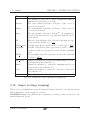
output
output precision
output k point
output eigenstate energy
potential solver
add constant potential
State solver
k points
number of k points
k space basis
kxmax, kymax, kzmax
kxmin, kymin, kzmin
k degeneracy
k0
integration order
NEMO5 User Manual
CHAPTER 5. SOLVERS AND OPTIONS
Description
Choose from Hamiltonian, energies, k-points, DOS,
electron density, electron density VTK, hole density,
hole density VTK,
ion density,
eigenfunctions,
eigenfunctions k0,
eigenfunctions VTK,
eigenfunctions VTK k0,
eigenfunctions Silo,
eigenfunctions Silo k0, spin.
Accuracy of saved eigenvalues within output file.
The (optional) name of the simulation object where the electrostatic potential is drawn from.
This option gives the possibility to add a constant potential
to the Hamiltonian.
Only relevant for calculate band structure. This parameter is a list of points in k-space along which the band structure
is calculated.
This list gives the uniform discretization of each segment set
by the k points parameter (note that specifying N points
means N − 1 segments). For density calculations, setting this
parameter to 0 leads to computation of k = 0 only and application of an analytical formula that assumes parabolic subbands.
(Default: cartesian) Sets the basis in which k points is
specified. When set to reciprocal the coordinates given in
k points are assumed to be w.r.t. the reciprocal lattice veca2 ×a3
tors b1 = a1 ·(a
, etc.
2 ×a3 )
Boundaries in 2π
of the simulated k-space. kx , ky , kz then
a
range from 0 to this number.
(Default: 0).
The computed density is multiplied by this number to account
for k-space degeneracy. E.g. when kxmax and kymax are set
in a simulation with 2D k-space, k degeneracy should be 4.
-
35
5.7. Schroedinger
Parameter
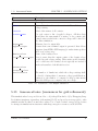
DOS energy grid
DOS min energy
DOS max energy
DOS points
DOS broadening model
DOS broadening
DOS spin factor
calculate elastic overlap
energy for elastic overlap
dE for elastic overlap
compute edges masses
compute edges masses delta
calculate brillouin zone
brillouin zone meshsize
minimum scattering angle
maximum scattering angle
electron temperature
electron chem pot
Dirac gaussian width
eigen values solver
number of eigenvalues
NEMO5 User Manual
CHAPTER 5. SOLVERS AND OPTIONS
Description
(for DOS calculation) Determines homogeneous energy grid
in the form (Emin,Emax,dE).
(for DOS calculation) alternative specification of Emin.
(for DOS calculation) alternative specification of Emax.
(for DOS calculation) alternative specification of the number
of energy points.
(for DOS calculation, default 2) 0: Lorentzian broadening, 1:
Exponential broadening, 2: cosh broadening.
(for DOS calculation) Broadening strength in eV.
(for DOS calculation, default 1) optional multiplicative factor
for DOS.
If set to true, some band edges and masses will be computed
and written to screen. This option was tested with bulk only
and fails to compute correct transverse masses for X- and Lvalleys in the presence of spin-orbit interaction.
(default: 0.001) stepsize for the finite difference scheme employe din compute edges masses, in π/a.
When set to true, the entire Brillouin zone will be meshed
and computed.
(default: 0.1) the spacing in every direction, in π/a (?).
Option connected to computation of scattering matrix elements, default 0.
Option connected to computation of scattering matrix elements, default 180.
(default: 1e-3) Which eigenvalue solver to use. Setting lapack always computes all eigenvalues and is feasible only for very small systems. Recommended choices are krylovschur and arpack.
Other choices are arnoldi, jd, gd.
Number of eigenvalues to compute (irrelevant for lapack).
36
5.7. Schroedinger
Parameter
linear solver
preconditioner
solver transformation type
max number iterations
convergence limit
monitor convergence
shift
fixed shift
mpd
ncv
mumps ordering
parallelize here
charge model
automatic threshold
spatially varying threshold
cutoff distance to bandedge
NEMO5 User Manual
CHAPTER 5. SOLVERS AND OPTIONS
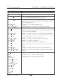
Description
Linear solver employed in the shift-and-invert operation. This
should be preferable a direct linear solver since the LU factorization can be reused during the Krylov iterations.
(default: lu) Preconditioner employed in the shift-and-invert
operation.
(default: sinvert) Use sinvert for shift-and-invert, shift
for shift.
Maximum number of Krylov iterations (irrelevant for
lapack).
Convergence limit for iterative solution methods (accuracy of
eigenvalues).
When set to true, terminal output related to the Krylov iteration is generated.
Eigensolver shift. Not sure when this is relevant, but only in
few cases.
Specialized numerical option. Refer to the SLEPc user manual
for the meaning.
Specialized numerical option (size of the Krylov subspace).
Relevant only for eigen values solver=mumps. Choose between pord and metis.
When set to false, some other simulation (like Propagator)
can determine the parallelization. (Default: true)
When set to electron hole (most cases), then an energy
threshold separates between electrons and holes. When set to
electron core model all states are assumed to be electrons.
If true, then the code determines the energetic threshold
that separates electrons and holes by looking at the bulk
band edges and the electrostatic potential. Preferred for
Schroedinger-Poisson simulations.
If true, then the threshold energy discriminating between
electrons and holes will vary spatially according to the electrostatic potential. Needed in Schroedinger-Poisson simulations.
Setting this to some value ∆ (in eV) leads to electron thresholds at Ec − eφ(x) − ∆ and hole thresholds at Ev − eφ(x) + ∆.
37
5.7. Schroedinger
CHAPTER 5. SOLVERS AND OPTIONS
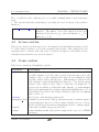
Parameter
threshold energy
Description
Energetic threshold above (below) which a quantum state
is regarded as an electron (hole). Instead of this option one can also use electron threshold energy and
hole threshold energy separately. These options are relevant only when automatic threshold is not true.
chem pot
Chemical potential (Fermilevel) in eV. Relevant only then
density is computed.
chem pot drain
(untested) when this option is specified, the states are populated in a top-of-the-barrier fashion (left- and right-traveling
states have different Fermilevels).
temperature
Temperature in Kelvin. Relevant only when density is computed.
epsilon matrix
Superimposed strain matrix ǫ in the laboratory system where
crystal axis might have been rotated.
epsilon matrix crystal
Superimposed strain matrix ǫ in the crystallographic system.
Options by R. Kotlyar, Intel:
These options were added to fix the shift of the eigenvalue
solver based on monitoring the subband energies from previous iterations. Usually these shifts are determined by conduction or valence band minima/maxima. Roza found that this
convergence scheme works the best for high electric fields in
the presence of large local band bendings.
calculate integrated hole density
If option is specified and spatially varying threshold = false,
the integrated the total carrier density in cm−dim is computed
by integration over the confinement dimensions (e.g. for wires
this yields 1/cm). As similar option exists for electrons.
calculate automatic shift subbandbased When true, the convergence scheme based on determining automatic shifts from subband energies is specified.
output shift subbandbased for restart
When true, at the end of simulation the file can be output
with the last eigensolver shift information. Using this shift
and the last potential, the next simulation can be restarted
from the last state of simulation.
input shift subbandbased for restart
When true, the shift is read in from file and is used as initial
shift to eigensolver.
input shiftfilename for restart
Filename for the above option.
kpoint to monitor subbands for shift
The k-point where to look for shift. default is 0.
kpoint tolerance to monitor subbands for shift
The k-tolerance when looking for a k-point on k-grid. Default
is 0.001.
NEMO5 User Manual
38
5.8. Semiclassical
CHAPTER 5. SOLVERS AND OPTIONS
Parameter
energy threshold for shift
rate of shift changes between iterations
Description
To determine the position of
eigensolver based on subband
To determine the position of
eigensolver based on subband
the next shift to be passed to
energies in previous iteration.
the next shift to be passed to
energies in previous iteration.
Table 5.6: Parameters of the Schroedinger simulation.
5.8
Semiclassical (semiclassical density)
This simulation can replace a more involved compuation of the density in some or all regions
of the structure by the simple semiclassical relationship
EF − (Ec − eφ(x))
n(x) = Nc F0.5
.
(5.1)
kT
This relation assumes a single parabolic conduction band with band edge Ec . F0.5 is the
Fermi integral of order 0.5. Nc is the effective density of states which is computed from the
effective mass and the band gap.
Parameter
Description
potential solver The solver from which the electrostatic potential φ can be
obtained.
fermilevel
The globally constant Fermilevel EF .
temperature
The temperature T in Kelvin (enters the Fermi function).
dimensionality
The density of states dimensionality. Default: 3.
Table 5.7: Parameters of the Semiclassical simulation.
5.9
WF (open-boundary wavefn. for ballistic transport)
Open-boundary wavefunctions are superior to the NEGF formalism when it comes to the
computation of ballistic transport properties. Simulation times are roughly 10 times faster.
The physics is, however, limited to ballistic simulations (no scattering).
Parallelism: The wavefunction solver has a three-level parallelization: energies, k-points,
and a spatial decomposition that is based on the numebr of contacts (using a generalized
NEMO5 User Manual
39
5.9. WF
CHAPTER 5. SOLVERS AND OPTIONS
recursive algorithm). In compination with Ramper this yields a 4D parallelization. Parallelization is done automatically except for the voltages.
Parameter
tb basis
Description
Tight-binding basis / band structure model. Can be em, s,
sp3sstar, sp3sstar SO, sp3d5sstar or sp3d5sstar SO.
potential solver
The name of the simulation where the electrostatic potential
is computed.
self consistent
(default: false) This boolean determines whether a selfconsistent iteration with the potential solver is done.
potential iteration
The maximum number of density-potential iterations at any
given bias.
constant potential
In the absence of potential solver this constant potential
is applied.
add constant potential
This quantity is added to the potential found by the electrostatic potential solver. Setting it may be required when the
initial guess of the potential is far away from the solution.
Setting a positive value means the conduction (and valence)
band will go down.
maximum potential variation Maximum update of the potential at any real-space point for
a single step.
potential criteria
Convergence criterion (norm of potential update vector).
Semiclassical
The (optional) name of a semiclassical density solver. When
set then this solver is iterated together with the potential
solver to obtain a selfconsistent initial guess for the potential.
use Semiclassical always
If true, then the Semiclassical solution will be used for the
initial guess of each bias step. Otherwise Semiclassical will
be called once at the begining of then simulation and the
potential solved in the previous bias step will be used as an
initial guess of the next bias step.
ramper name
The (optional) name of the Ramper simulation. If there is
none, one can specify the name of lead domains to apply biases.
resonance solver
The (optional) name of a ResonanceFinder simulation that is
used for adaptive energy grids. Such an object is mandatory
for RTD-type simulations where the energy grid needs to be
refined well around some resonances.
NEMO5 User Manual
40
5.9. WF
Parameter
contact self energy
Sr damping
Enum
Emin
Emax
bandgap margin
band margin
Edif
use adaptive grid
use adaptive grid1
use adaptive grid low
use adaptive grid high
use adaptive grid Fermi
Korigin
NEMO5 User Manual
CHAPTER 5. SOLVERS AND OPTIONS
Description
Determined by which method the contact self-energy is calculated. All methods should give the same but their speed is
differnet. For WF and NEGF the default choice is M for tightbinding and MS for single-band effective mass simulations. (M
stands for Mathieu Luisier). For NEGF two additional choices
are available: SR (Sancho-Rubio) and T (Tillmann Kubis).
Numerical parameter (in eV) for a small imaginary part of
the contact Green’s functions. This will lift singularities at
the band edges.
Initial number of energy points. During the simulation this
number can change according to refinement around a resonance (which is found using a ResonanceFinder simulation).
Minimal computed energy in eV. When not set then this will
be computed automatically.
Maximum computed energy in eV. When not set then this
will be computed automatically.
When Emin is not set then Emin = minx (Ec −
eφ(x))−bandgap margin (for n-type). Default is 15kT .
When Emax is not set then Emax = maxx (Ec −
eφ(x))+band margin (for n-type). Default is 25kT .
−Emin
.
If Enum is not specified but Edif, then Enum = EmaxdE
When set to false then a homogeneous energy discretization is
used. This option does not change the total number of energy
points. (Default: true)
When set to true then more energy points are added (Default:
false)
Introduce refinement around the minimum band edge. The
given value is the weight associated to the refinement. (Default: true).
Introduce refinement around the maximum band edge. The
given value is the weight associated to the refinement. This
might be useful for p-type semiconductors. (Default: false).
Introduce refinement around the Fermilevels. The given value
is the weight associated to the refinement. (Default: true).
The center k0 of k-space, in units of πa . For direct-gap materials this should be 0, for Silicon electron devices this should
be somewhere near the X-minimum.
41
5.9. WF
Parameter
Kradius
Knum
Kdeg
analytical k space
RTD simulation
output name
output
CHAPTER 5. SOLVERS AND OPTIONS
Description
The extension in each direction, as a fraction of the Brillouin
zone extension. (For a 2D k-space 0.1 will have kx and ky vary
between (k0x − 0.1 πa , k0y − 0.1 πa )) and (k0x + 0.1 πa , k0y + 0.1 πa )).
k-space will be discretized into (2Knum + 1)d pieces, where
d is the dimension of periodicity. Set to -1 in order to use
an analytical k-space formula that assumes parabolic bands
(Then only k = 0 needs to be computed and the Korigin and
Kradius options are irrelevant).
Factor by which the obtained density is multiplied due to
degeneracies in k-space.
When set to true then a log(1 + x) formula will be used in
the case when only k=0 is solved (Knum=-1). The obtained
energy-resolved quantities will only show the k=0 quantity,
so the energy axis is in a sense not the total energy anymore.
When set to false then a numerical scheme is used so energyresolved quantities will show all k-values for any given (total)
energy, assuming effective mass.
(Default: false) if true, then the entire Hamiltonian is stored
in memory. This is possible for 1D simulations and may bring
about a speed up.
Name for generated output files.
Atom-based output to be generated in the end. Can be
transmission, potential, free charge, free charge cm-3,
current,
electron energy (average electron energy
R
dE
En(x,E)
R
) and hole energy.
dE n(x,E)
1D output that is interpolated onto an axis and can be
viewed as 1D graphs in e.g. Matlab. Can be potential or
free charge.
one dim output average
If true, then the atomic values are averaged over a unit cell.
If false then the atomic positions form the basis of the 1D
discretization.
option, option1, option2
PETSc linear solver option name, e.g. -ksp type or -pc type.
option value, ...
PETSc linear solver option value, e.g. preonly or lu.
Table 5.8: Parameters of the WF and NEGF simulations.
one dim output
For NEGF and WF transport simulations, separate Domains are needed for the device
NEMO5 User Manual
42
5.10. NEGF
CHAPTER 5. SOLVERS AND OPTIONS
and each lead. In the device domain, the lead domains need to be specifies via
leads = (lead1name, lead2name).
In the lead domains, one needs to specify the outward direction and the type of lead. For an
example, if the outward direction is the opposite of crystal direction2:
lead direction = {-1, 1, -2, 2, -3, 3} . // Then the doping type of the leads needs
to be specified: lead type = N, P .
Parameter
Description
option2 value Choice of linear solver when option2 is not specified explicitly. Set e.g. to mumps or superlu dist.
Table 5.9: Additional parameters of the WF simulation.
5.10
NEGF (semi-coherent transport)
The implementation of Nonequilibrium Green’s Functions (NEGF) has a lot of things in
common with the WF implementation. It shares all the parameters except that type is
NEGF instead of WF. It also has the same MPI-parallelism. There are additional parameters
connected to scattering:
Parameter
scattering
Description
When set to true then a scattering model is turned on based
on deformation-potential scattering with phonons.
phonon factor atom Debug option to adjust the electron-phonon interaction
strength in the deformation potential model. Do not use.
density iteration Maximum inner iterations (Green functions - self energies)
symmetric
(default: false) When set to true then matrices are saved in a
symmetric format.
Table 5.10: Additional parameters of the NEGF simulation.
5.11
TopOfBarrier (transport using top-of-the-barrier
model)
This is Mark Lundstrom’s famous top-of-the-barrier model [7]. It allows for the rapid calculation of I-V curves and other characteristics of ballistic nanotransistors gien that the density
NEMO5 User Manual
43
5.11. TopOfBarrier
CHAPTER 5. SOLVERS AND OPTIONS
of states (DOS) and the average carrier velocity (vavg) is known from another simulation.
Alternatively the DOS and vavg it can be computed by this simulation given knowledge of
the E(k).
Parameter
Ek file
Description
Name of a file containing E(k) in the format kx ky kz E1 E2
... Specifying this option overrides DOS file and vavg file.
This file is typically generated by a Schroedinger simulation
(ending energies.dat).
Emin
(if Ek file is used, in eV) Energy minimum of the regular
grid set up for D(E) and vavg(E).
Emax
(if Ek file is used, in eV) Energy maximum of the regular
grid set up for D(E) and vavg(E).
dE
(if Ek file is used, in eV) Energy spacing of the regular grid
set up for D(E) and vavg(E).
broadening
(if Ek file is used, in eV) Every energy eigenvalue is broadened by this amount to smoothen the DOS and vavg curves.
k deg
(if Ek file is used) The computed DOS is multiplied by this
number to account for degeneracy in k-space. Like this it
suffices typically to compute half or 1/4 of the Brillouin zone.
spin deg
(if Ek file is used) The computed DOS is multiplied by this
number to account for spin degeneracy.
gradient dir (if Ek file is used) Direction in which the velocity is computed. The direction is specified in terms of the reciprocal
lattice vectors and should have dim components.
DOS file
Name of a file containing the density of states in the format
E D(E).
vavg file
Name of a file containing the energy-resolved average velocity
in the format E vavg(E). The energy grid must be the same
as for the DOS.
drain bias
Vector containing the voltages applied to the drain contact.
gate bias
Vector containing the voltages applied to the gate contact.
Must have the same length as drain bias.
temperature The temperature in Kelvin.
dim
The dimensionality of the problem: 1 for a nanowire or fin
geometry, 2 for a thin body. This must be in agreement with
Ek file if that option is used.
NEMO5 User Manual
44
5.12. Ramper
CHAPTER 5. SOLVERS AND OPTIONS
Parameter
EF
Csource
Cdrain
Cgate
EOT
double gate
tripleQW
EOT QW
Description
The Fermilevel of the source contact. Raising this results in
shifting the ID (VG )-curve to the left.
The source-channel capacitance, in F/mdim . Can be set to 0
for ideal electrostatics.
The drain-channel capacitance, in F/mdim . Can be set to 0
for ideal electrostatics.
The gate-channel capacitance, in F/mdim . It is unusual to
specify it like this, therefore a specification with EOT can be
made instead.
Effective oxide thickness of the dielectric separating the gate
3.9ǫ0
contact and the channel: CG = EOT
.
3.9ǫ0
(default: false) If true, then CG will be doubled (CG = EOT
).
(default: false) If true, then a special model will be turned
on that accounts for capacitances between the three quantum
wells.
(if tripleQW is used) The capacitance between two wells will
3.9ǫ0
be CQW = EOT
QW
Numerical parameter to adjust the maximum number of Newton iterations in the solution for U .
Numerical parameter to adjust the maximum update per
Newton step in the solution for U .
Numerical parameter to adjust the convergence criterion in
the solution for U .
The output file where all results will be written to.
Table 5.11: Parameters of the TopOfBarrier simulation.
max iters
dUmax
Utol
file
5.12
Ramper (voltage ramping)
This is a top-level simulation to run selfconsistent density-potential (or any other) iterations
while ramping the voltages applied to contacts.
Parallelism: Ramper can parallelize the computation of voltage points, if desired (see the
parallelization option).
NEMO5 User Manual
45
5.13. ResonanceFinder
Parameter
CHAPTER 5. SOLVERS AND OPTIONS
Description
Parameter
solver
Description
Name of the solver whose solve-routine shall be called at every
voltage setting.
contacts
A list of the names of all contacts.
<contact name>
For each contact a list of applied voltages. All these lists
should have the same number of entries, or else contain only
a single entry at which the contact’s voltage will be fixed for
the entire simulation.
output name
Filename base for output files.
rappture output
If true then some terminal output is generated that allows
Rappture (nanoHUB’s GUI language) to make status updates
after every voltage step.
density solver
Name of the density solver.
call density solver output If set to true, then the output routine of the density solver
is called in each voltage setting. This routine would normally
not be called since the density solver is typically not included
in the solvers list of the Global section.
current solver
potential solver
parallelization
The number of chunks into which the voltage settings shall
be divided. Setting this to 1 means no voltage parallelization,
setting it to the number of computed voltage points means
that each MPI process computes only one voltage.
Table 5.12: Parameters of the Ramper simulation.
5.13
ResonanceFinder (resonances for grid refinement)
This simulation has been ported from older code (rtdnegf Nanohub tool) by Zhengping Jiang.
It calculates imaginary eigenvalues of the matrix (H +Σ) and provides an energy grid to other
simulations that is refined around these values. Use of such a refined energy grid is decisive
for transport simulations in structures with sharp energetic resonances, such as RTDs.
NEMO5 User Manual
46
5.13. ResonanceFinder
CHAPTER 5. SOLVERS AND OPTIONS
Parameter
Description
Parameter
density solver
Description
Name of density solver simulation which will provide information about Hamiltonian, initial energy grid etc.
Starting slab of resonance finding region. 0 = first slab of
quantum region within range [0, N). N is the number of slabs
in the quantum region.
Ending slab of resonance finding region.
Maximum number of iterations in Newton refinement.
Number of points for homogenous grid.
Number of points for resonance peak and also imaginary part
of retarded Green’s function.
Number of points for real part of retarded Green’s function.
Number of points to refine two sides of retarded Green’s function peak. This is defined to be side peak.
Number of points to refine real part of side peak.
Number of points for fermi level.
Number of points for derivative of fermi level.
Number of points for conduction band and 1D density of
states.
Number of points for phonon retarded Green’s function.
Number of points for real peaks of phonon retarded Green’s
function.
Maximum number of Lanczos iterations.
Parameter used to refine conduction band.
Parameter used to refine conduction band.
-.
-.
-.
-.
-.
-.
-.
-.
-.
starting cell
ending cell
iteration limit1
node homo
node res
node real res
node res2
node
node
node
node
real res2
fermi
dfermi
cb
node pho res
node pho real res
num lanczos
Ehi
gamma
Newton step
Newton converge
scale factor
exclusion slabs
init step
print all
Emin, Emax
total k
output
NEMO5 User Manual
47
5.14. Angel
CHAPTER 5. SOLVERS AND OPTIONS
Parameter
output name
Description
-.
maximum resonance number -.
Table 5.13: Parameters of the ResonanceFinder simulation.
5.14
Angel (NEGF plugin)
This simulation type is a port of Sebastian Steiger’s NEGF solver ANGEL1 [8]. It is not yet
functional.
Parameter Description
Table 5.14: Parameters of Angel.
5.15
MatrixElements (matrix elements between wavefunctions)
This simulation calculates matrix elements between quantum states as a post-processing step.
It relies on another simulation which calculates the wavefunctions and is specified using the
parameter wf simulation.
The general idea is that given two states |ψ1 i and |ψ2 i, the calculation of
|hψ2 |Â|ψ1 i|2 ≡ |hψ2 ||ψ̃i|2
(5.2)
looks similar for all operators Â. All that has to be implemented is the calculation of
|ψ̃i ≡ Â|ψ1 i.
Parameter
operator
wf simulation
1
Description
Determines the type of matrix element to calculate. One of
overlap or optical.
The name of the simulation from which eigenfunctions and
eigenenergies are obtained (e.g. a Schroedinger simulation).
http://nanohub.org/resources/8136
NEMO5 User Manual
48
5.16. Brillouin
Parameter
output file
CHAPTER 5. SOLVERS AND OPTIONS
Description
The base name for output files.
Optical matrix element parameters (operator=optical):
transition
polarization phis
polarization thetas
Parameters for
absorption
egrid size
gamma
the quantum dot lab application (operator=optical):
If true, an absorption plot α(~ω) will be generated.
The number of photon energy (~ω) grid points.
Linewidth of the Lorentzian broadening of the transitions, in
eV.
sweep
Depending on its value (angle, temp ,ef), a family of absorption plots is generated by sweeping either the polarization
angle, the temperature or the Fermilevel.
sweep values
Number of values of the sweep quantity.
temp
Vector. The first entry determines the temperature; if
sweep=temp, all subsequent values are the sweep values.
ef
Vector. The first entry determines the Fermilevel; subsequent
values are the sweep values if sweep=ef.
Table 5.15: Parameters of the MatrixElements simulation.
5.16
Brillouin (computation of Brillouin zones)
This simulation determines the Brillouin zone (BZ) of the given unit cell and saves it to file.
• Only the specification of the unit cell via crystal directionN matters for the calculation. The size of the total structure, be it one or multiple unit cells, is irrelevant.
The
• BZs of supercells can be constructed by enlarging the crystal directionN correspondingly.
• The saved structure always has its coordinates in Cartesian space.
• The result is currently always located in the file BZ.vtk
NEMO5 User Manual
49
5.17. DriftDiffusion
CHAPTER 5. SOLVERS AND OPTIONS
Parameter Description
output file VTK file where the 3D body will be saved. Please omit the
.vtk-ending in this option.
Table 5.16: Parameters of the Brillouin simulation.
5.17
DriftDiffusion
This simulation solves the stationary continuity equation ∇ · J = G − R, where the current
density J is expressed by the combination of drift and a diffusion term.
Parameter
Description
poisson solver Name of the simulation that provides Poisson solver.
Table 5.17: Parameters of the DriftDiffusion simulation.
5.18
Propagation (general NEGF solver)
This simulation is an attempt to set up a general NEGF framework for electron and phonon
systems. It is still under heavy development.
Parameter
Hamilton constructor
Parallelizer
reuse parallel hierarchy
top most MPI strategy
number of k points
kxmax,kymax,kzmax
Description
Name of the simulation that generates the Hamiltonian.
Name of the simulation that determines the parallelization
Vector
Can be cluster (default) or scatter. Refer to the N5 paper
[1] for an illustration of these strategies.
Vector of names for “momenta”, i.e. k,E,...
If true, then ...
A vector that may contain the following bits. 1. Either
“Green” or “self”. 2. “inverse”, “lesser”,“greater”,“retarded”
or “advanced”. 3. “Fermion” or “Boson”.
-
NEMO5 User Manual
50
momentum names
X constructor
X points
transmission
NEGF object list
5.18. Propagation
CHAPTER 5. SOLVERS AND OPTIONS
Parameter
chemical potential
temperature
G for transmission
Description
selfenergy1 for transmission
selfenergy2 for transmission
Same as selfenergy1 for transmission.
density of
Table 5.18: Parameters of the Propagation simulation.
5.18.1
Greensolver (subtype of Propagation)
This is a helper simulation.
Parameter
do output
X inversion
Hamilton constructor
stationary Propagation
Hamilton momenta
Table 5.19:
5.18.2
Description
If true (default), then..
Parameters of the Greensolver simulation.
Self energy (subtype of Propagation)
This is a helper simulation.
Parameter
equilibrium model
stationary Propagation
do output
constant eta
iterative damping
retarded lead method
Hamilton constructor
transfer lead direction
NEMO5 User Manual
Description
If true (default), then ...
If true (default), then..
If true (default: false), then...
Optical potential.
(Default: 0.5)
One of direct iterations (default), transfer matrix or
Sancho-Rubio.
Integer that can take the value +1 or -1.
51
5.20. Contacts
CHAPTER 5. SOLVERS AND OPTIONS
Parameter
LRA
Description
(Default: false) indicates whether a low-rank approximation
is performed.
translate to device domain
(Default: false)
target Hamilton Constructor Table 5.20: Parameters of the Self energy simulation.
5.19
SimulationModules (helper for Propagation)
This helper combines various simulations into logical units to ease input deck creation.
Parameter
Description
Module type
job list
tb basis
lead direction
lead domain
momentum names
X constructor
Hamilton momenta
do output
max num iterations Table 5.21: Parameters of the SimulationModules simulation.
5.20
Contacts (helper for Propagation)
This is a helper simulation that computes NEGF quantities related to contacts.
NEMO5 User Manual
52
5.20. Contacts
CHAPTER 5. SOLVERS AND OPTIONS
Parameter
Description
Hamilton constructor Name of the simulation that provides the Hamiltonian.
potential solver
Name of the simulation that provides the electrostatic potential (typically a Poisson solver).
job list
A vector that may contain the following: assemble H,
get hamiltonian,
passivate H,
calculate sigmaR,
calculate sigmaL, calculate left moving leadstates,
calculate right moving leadstates,
calculate surface GL, calculate surface GR.
Table 5.22: Parameters of the Contacts simulation.
NEMO5 User Manual
53
Chapter
6
Material Parameter
Names
This chapter is a reference on which material parameters are relevant for which solver.
Ramper, ResonanceFinder, Propagation, Angel, MatrixElements simulations:
These simulations are either dysfunctional or they do not directly implement a physical
equation. Hence there are no material parameters associated with them.
6.1
Structure, Brillouin
These simulations depend only on the atomic grid and hence are only dependent on the
parameters forming the grid. All these parameters are located in the Lattice group of the
material database.
Crystal structure
simple cubic
diamond, zincblende
wurtzite
Bi2Te3
Parameter
a lattice
a lattice
a lattice, a wurtzite, c wurtzite
a lattice, c lattice, u lattice, v lattice
Table 6.1: Material parameters relevant for atomistic grid construction.
54
6.2. VFFStrain, Phonons
6.2
CHAPTER 6. MATERIAL PARAMETER NAMES
VFFStrain, Phonons
In the following table X always denotes the name of an atom, i.e. Si, Ga, As etc. All parameters
are located in the Lattice group in the material database.
Parameter
strain alpha
strain beta OR
strain beta X
Description
Keating’s bond-stretching parameter α.
Keating’s bond-bending parameter β.
If a separate parameter strain beta X is present for all atom
types X than those will be used instead.
strain gamma OR
Cross-stretch interaction parameter.
strain cross stretch X If separate parameters are present for all atom types then
those will be used.
strain delta OR
Stretch-bend interaction parameter.
strain stretch bend X If separate parameters are present for all atom types then
those will be used.
strain nu
Second-nearest-neighbor coplanar interaction parameter.
strain anharm ...
Anharmonicity parameters used in the Lazarenkova, Areshkin
or Sui/Herman anharmonicity models.
X charge
Fractional point charge sitting at the atomic locations that
induces a Coulomb interaction.
X mass
Atom mass in amu., used only in dynamical matrix (phonons)
Table 6.2: Material parameters relevant for the VFFStrain and Phonons simulations.
6.3
Poisson, NonlinearPoisson
For the Poisson equation only the static dielectric constant is needed.
Crystal structure
Parameter
simple cubic,diamond, zincblende Lattice:epsilon dc
wurtzite, Bi2Te3
Not yet implemented.
Table 6.3: Material parameters relevant for the Poisson and NonlinearPoisson simulations.
NEMO5 User Manual
55
6.4. Schroedinger, WF, NEGF
6.4
CHAPTER 6. MATERIAL PARAMETER NAMES
Schroedinger, WF, NEGF
These simulations are all centered around the electronic Hamiltonian, and thus the following
parameters are needed:
• Tight-binding or effective-mass parameters for the Hamiltonian.
• For tight-binding simulations where an analytical formula is used to compute the density from k = 0 results, effective-mass parameters are also used.
The nomenclature for tight-binding parameters is consistent and straightforward to interpret.
For example, E Sstar Ga denotes the onsite energy of the s∗ orbital and V S P Sigma As Ga
is the σ-coupling element between the arsenic s-orbital and the gallium p-orbital. Note that
when entries are symmetric (e.g. V S S Sigma X Y must always be the same as V S S Sigma Y X)
then only a single entry is used where the atomic sorts X and Y are ordered alphabetically.
Effective-mass simulations are currently implemented with a fake tight-binding model using
a single s-orbital.
Parameter
Description
tight-binding parameters The parameter sets are located in the group
Bands:TB:<tbmodel>:param XYZ,
where
<tbmodel>
corresponds to the model given in the input deck
(e.g. sp3sstar SO) and param XYZ is the name of the
employed parameter set (e.g. param Klimeck).
Ec, Ev
Located in Bands:BandEdge. These parameters are used for
the distinction between electrons and holes.
mstar {c,v} dos
Located in Bands:BandEdge. These parameters are used in
effective-mass simulations and when computing the density
fom k = 0-results assuming a parabolic transverse dispersion.
Table 6.4: Material parameters relevant for the Schroedinger, WF and NEGF simulations.
Choice of tight-binding parameter sets
This choice can be made by setting Bands:TB:<tbmodel>:param set = param XYZ in the
Material section in the input deck.
Valence band offsets
Valence band offsets can be adjusted either directly in the material file (typically all.mat)
by changing the parameter Bands:BandEdge:VBO or Bands:TB:<tbmodel>:param XYZ:VBO,
or they can be adjusted by setting the same parameter in the corresponding Material section
in the input deck. The onsite tight-binding energies will then be shifted by a constant value.
NEMO5 User Manual
56
6.5. Semiclassical
6.5
CHAPTER 6. MATERIAL PARAMETER NAMES
Semiclassical
All the Semiclassical material parameters are located in the group Bands:BandEdge.
Parameter
Description
Ec, Ev
Bulk conduction and valence band edge.
mstar c dos, mstar v dos Density-of-states masses.
Table 6.5: Material parameters relevant for the Semiclassical simulation.
NEMO5 User Manual
57
Bibliography
[1] S. Steiger, M. Povolotskyi, T. Kubis, H.-H. Park and G. Klimeck, Manuscript accepted
to IEEE Transactions of Nanotechnology (2011).
[2] R. Lake, G. Klimeck, R. C. Bowen and D. Jovanovic, J. Appl. Phys. 81, 7845 (1997).
[3] G. Klimeck et al., IEEE Trans. Electr. Dev. 9, 2079 (2007).
[4] G. Klimeck et al., IEEE Trans. Electr. Dev. 9, 2090 (2007).
[5] M. Luisier, A. Schenk, W. Fichtner and G. Klimeck, Phys. Rev. B 74, 205323 (2006).
[6] A. Trellakis, A. T. Galick, A. Pacelli and U. Ravaioli, J. Appl. Phys. 81, 7880 (1997).
[7] A. Rahman, J. Guo, S. Datta and M. Lundstrom, Electron Devices, IEEE Transactions
on 50, 1853 (2003).
[8] S. Steiger, R. G. Veprek and B. Witzigmann, Electroluminescence from a quantum-well
led using negf, in International Workshop on Computational Electronics (IWCE), Beijing,
2009, IEEE.
58