Download Toolkit User manual - LEDS Global Partnership

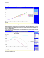
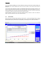
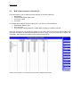
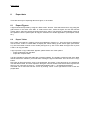
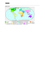
User Manual
Information Toolkit for post-2012 climate policies
Version 2009
Authors
Sander Brinkman (Brinkman Climate Change)
Koen Smekens (ECN Policy Studies)
Page 2 of 15
Name, address of corresponding author
Sander Brinkman
Brinkman Climate Change
Theresiastraat 133b
2593AG DEN HAAG, The Netherlands
E-mail: [email protected]
Koen Smekens
ECN Policy Studies
Netherlands
Tel: +31-(0)224-564861
E-mail: [email protected]
Disclaimer
Statements of views, facts and opinions as described in this report are the responsibility of the author(s).
It is not allowed to use the model and/or its results for commercial purposes. The Toolkit team is not
obliged to offer any technical support of the AIMMS software.
It is not allowed, without written permission of the Toolkit’s developers, to distribute, license, or otherwise transfer the Toolkit to any other individual or institution; alter, modify, enhance or otherwise
change the Toolkit; or use the Toolkit in conjunction with any other computer software.
Toolkit’s developers will not be liable for any indirect, special or consequential damages in connection
with or arising from the provision of, performance of or use of the Toolkit.
Copyright © 2009, ECN, Petten
All rights reserved. No part of this publication may be reproduced, stored in a retrieval system or
transmitted in any form or by any means, electronic, mechanical, photocopying, recording or otherwise
without the prior written permission of the copyright holder.
Page 3 of 15
Contents
1.
Toolkit installation
1.1
Hardware and operating system requirements
1.2
Download software
1.3
Download datasets
4
4
4
4
2.
Contents of the Toolkit
5
3.
Start and browse
3.1
Start
3.2
Browse
7
7
8
4.
Info button
8
5.
Create figures and tables
5.1
Create figures
5.2
Create tables
5.3
Multi criteria selection countries (Vi)
9
9
11
12
6.
Export data
6.1
Export Figures
6.2
Export Tables
13
13
13
Appendix, Abbreviation of regions
14
Page 4 of 15
1.
Toolkit installation
The Toolkit is a computer-based information system that contains flexible factsheets, including tables,
figures and graphs. It is built in AIMMS software (AIMMS3.9 Viewer, www.aimms.com,). AIMMS enables users to easily show large datasets in graphs and to easily add or remove parameters. The
Toolkit brings together data and information from various national and international sources and integrates them into one system.
1.1
Hardware and operating system requirements
The hardware requirements are:
• 1.6 Ghz or higher x86 or x64 processor
• XGA display adapter and monitor
• 1 Gb RAM
• 1 Gb free disk space
When you try to run an Aimms project for larger data sets on a PC with a small amount of installed or
available RAM, you may find that the increased memory requirements of running large models give
rise to extensive disk swapping. In general, this will have a dramatic effect on the overall performance
of both Aimms and the other applications running concurrently with Aimms. In such a case you are
advised to install sufficiently additional RAM to run all applications comfortably again.
The Aimms 3.9 Viewer is designed to run under
• Windows 2000,
• Windows XP,
• Windows Server 2003, and
• Windows Vista.
1.2
Download software
Please visit the AIMMS website: http://www.aimms.com
Then go to DOWNLOADS AIMMS Viewer 3.9.2
Once the software has been installed, an AIMMS Viewer icon is displayed on the desktop.
It must be emphasised that you need administrator rights to be able to download software on your
computer. Please be aware the software creates a new directory: c:/ program files / Paragon Decision
Technology.
1.3
Download datasets
The contents of the Toolkit (prj–file), the datasets, can be downloaded from
http://www.brinkmanclimatechange.com/Toolkit.htm. Please create a Toolkit directory on the local
desktop to save the (prj) file. If the contents are put in a zip-file, please right-click on it, and choose
“unpack all”. Once saved, double click on the AIMMS Viewer icon on the desktop. The Viewer opens,
and an existing project (prj) can be opened.
Please browse, locate and click on the Toolkit file in the Toolkit directory created in the previous step.
After closing the software the path to the prj will be saved by the viewer. The next session will automatically open with this project. A project list is visible in the main screen when a new session of
AIMMS is started.
Now the Toolkit opens in a new window and should run properly. If not, please try the whole procedure
again. If the problem is persistent, please contact the developers of the Toolkit.
Page 5 of 15
2.
Contents of the Toolkit
The subjects covered in the Toolkit (Version 2009) are:
Ia - IPCC Stabilisation Categories
Ib - Characteristics of Greenhouse gas Stabilisation scenarios
Ic - Characteristics of post-TAR stabilisation scenarios
Id - Stabilisation targets and chance of meeting temperature target
Ie - Temperature Change
If - Emission envelopes for stabilisation at 450 550 and 650
Ig - Peaking and stabilization concentration profiles
Ih - Emission pathways for meeting stabilisation targets
Ii - Implications of delaying global actions for emission pathways
Ij - Global corridors for meeting long-term stabilisation levels
Ik - Reduction target ranges for stabilization scenarios
Il - Trade off reduction non Annex I
Im - Trade off Annex I against non Annex I
In - Impact of deforestation on trade-off Annex I non-Annex I
IIa - Indicators
IIb - Short term projections
IIc - Scenario Intensity Indicators
IId - Shares in GHG development
IIe - Emission reduction gaps for 2020 and 2050
IIf - Projections of non Annex I emissions
IIg - GHG emission with frozen and baseline technology
IIh - Bunker emissions
IIi - Baseline projections of marine bunker emissions
IIj - Share of marine bunker emissions
IIk - Projections of global marine bunker emissions
IIl - Projections of global land use emissions of CO2
IIm - Global projections and trends versus IPCC scenarios
IIn - National Targets Kyoto Protocol
IIo - IMO CO2 Emissions
IIp - Factors underpinning Future Actions Trajectories
IIq - Simple climate fact sheets per country
IIIa - Global economic mitigation potential 2030
IIIb - Sectoral economic mitigation potential 2030
IIIc - Global Business as Usual and reduction potential for different sectors
IIId - TDBU Savings Bottom Up compared to IPCC AR4
IIIe - TDBU Savings Top Down compared to IPCC AR4
IIIf - TDBU Relative emission reduction compared to baseline for 2030
IIIg - TDBU Relative emission reduction compared to baseline for 2030, per sector
IIIh - TDBU Relative emission reduction compared to potential in 2030
IIIi - Cumulative emission reduction
IIIj - Cumulative emission reductions up to 2100
IIIk - Mitigation strategies
IIIl - Share of renewable energy in primary energy supply
IIIm - Electricity production indicators 2005
IIIn - Steel production - CO2 reduction potentials and indicators
IIIo - Cement production - CO2 reduction potentials and indicators
IIIp - Mitigation Potential Forestry TDBO AR4
IIIq - Mitigation Potential Forestry AR4
IIIr - Mitigation Potential Forestry for 20 and 50 US$
Page 6 of 15
IIIs - Cost of achieving mitigation potential
IIIt - LULUCF mitigation scenarios
IIIu - Carbon price and mitigation costs from meat consumption scenarios
IIIv - GHG and Land Use Change emissions from meat consumption scenarios
IIIw - Meat consumption scenarios
IIIx - Marginal costs of emission reductions with AD activities
IIIy - ADAM emission scenarios
IIIz1 - GAINS GHG emissions
IIIz2 - GAINS sector emissions
IV-Aa - Global abatement cost as % of GDP for meeting pathways
IV-Ab - Global abatement costs as % of GDP
IV-Ac - Estimated global macro-economic costs in 2030 and 2050
IV-Ad - Net Present Value of abatement costs
IV-Ae - NPV abatement cost levels
IV-Af - Regional abatement costs as % of GDP in 2020 and 2050
IV-Ag - Permit price for 450 and 550 ppm
IV-Ah - POLES reference scenario abatement cost for European countries (2010 and 2020)
IV-Ai - Global cost curve
IV-Aj - OECD mitigation adaption costs
IV-Ak - OECD mitigation costs comparisons models
IV-Al - Global impacts of climate change
IV-Am - WAB balancing carbon price 2010
IV-An - WAB balancing carbon price 2020
IV-Ao - EMF global cost delay
IV-Ap - EMF China cost delay
IV-Aq - Annex I carbon prices 2020
IV-Ar - Carbon price developments over time in the global carbon market (€ per ton CO2)
IV-As - McKinsey aggregate reduction vs 1990
IV-At - McKinsey cost curve
IV-Au - McKinsey financial flows
IV-Av - ADAM carbon price
IV-Aw - ADAM GDP loss
IV-Ax - GAINS Total costs
IV-Ba - Regional MAC curves
IV-Bb - MAC curve 2020
IV-Bc - MAC curves POLES model for 2020
IV-Bd - Marginal CO2 prices
IV-Be - EMF MAC curves USA 2020 and 2050
IV-Bf - IIASA MAC curves relative to baseline
IV-Bg - GAINS MAC curves
IV-Ca - CDM Market potential excluding avoided deforestation
IV-Cb - Theoretical Global CDM Cost Curves incl. and excl. deforestation
IV-Cc - Country Regional CDM Cost Curves
Va - Mitigation potentials and costs on a country basis
Vb - Energy related R and D expenditures on a country basis
Vc - Energy import dependency in scenarios
Vd - UN Human Development Index
Ve - Historic Responsibilities
Vf - Reduction of SO2 and NOx emissions compared to the baseline
Vg - Reduction of air pollutants due to GHG mitigation
Vh - Avoided external costs due to GHG mitigation
Vi - Multicriteria Selection Countries
Page 7 of 15
3.
Start and browse
3.1
Start
When starting the Toolkit, the opening page will be shown.
Opening page
On the opening page 4 menu options are displayed: File, Edit, About, Toolkit. These menus will be
available at all times when using the Toolkit:
File
In the file menu 3 functions are included. Two are for printing, one is “Print Setup” containing the
printer identification and selection, the other is “Print” which sends the current view to the selected
printer. The last one, “Exit”, is to exit the Toolkit Viewer.
Edit
The “copy” function will be enabled when tables are shown. This function enables the user to copy the
datasets as given in the table directly into other software such as Word or Excel.
The “Grab screen” function for exporting figures to other applications. See chapter 6.
About
Information about the AIMMS software and Toolkit version.
Page 8 of 15
Toolkit
This menu item contains all subjects covered by the Toolkit. It can be be used to navigate to other
pages in the Toolkit (see section 3.2). By clicking the “About Toolkit” option, users return to the opening screen.
The “Show table” function, when enabled, shows the data included in the figures in a table. The data
shown can be exported as explained later (See chapter 6).
3.2
Browse
Use the “Toolkit” function in the top-menu for browsing through the Toolkit. When clicking on “Toolkit”,
a list of subjects covered in the Toolkit is shown. There are currently 5 main levels. Please scroll
through the menu and choose the subject of choice.
A second way to browse through the Toolkit is to enter one of the five main categories by clicking on
one of the five buttons at the main screen:
The five main categories
Once entered the main category, the following functions at the bottom are shown:
Browsing through the five main categories
The figure above shows the five main categories. The categories can be changed by clicking on the I,
II, III, IV or V. For browsing within a main category click on the < or >.
4.
Info button
For every figure an info button is provided.
Clicking on this button will open an pdf file - external to the Toolkit - which shows:
1) Relevant background information on the datasets and on the displayed information
2) Source information: reference to articles or reports, and a website address when available,
oncerning the displayed information.
Page 9 of 15
5.
Create figures and tables
There are different types of figures in the Toolkit with different flexibilities and functions as explained
below.
5.1
Create figures
Hard coded figures
e.g. Toolkit I : Emission pathways and corridor analysis Ic : Emission envelopes for stabilisation
at 450, 550 and 650
Example hard coded figure
These figures are copied from articles, reports or websites. The figures can only be copied into other
applications e.g. Powerpoint or Word document by using the Edit- Grab Screen function.
Page 10 of 15
Flexible Figures
Type 1, e.g. Toolkit I : Emission pathways and corridor analysis Ie : Temperature change
Figure 5.1: Example of a limited flexible figure
On the right hand side there is a scroll menu headed with “Scenarios”. Please select one or more stabilisation scenarios to display. For selecting several scenarios, please use CTRL and click on the scenarios. For selecting a number of consecutive scenarios, please click on the first and use SHIFT while
clicking on the last scenario.
Type 2, e.g. Toolkit I : Emission pathways and corridor analysis Ie : Emission pathways for meeting stabilisation targets
Example of a fully flexible figure.
Page 11 of 15
This is the maximum flexibility you can get. Please be aware you first have to choose whether you
want to show the emission pathways per sector, per gas, per region or per scenario (at the bottom of
the figure).
If you choose to show the figure by region, all contributions will be shown per region. However, if you
choose to select the gases CH4 and CO2 at the same time, these will be shown together as a sum, instead of separated. So if you want to show the gases separately, you have to choose to show the figure by gases, instead of by regions (option buttons below the figure).
Another flexibility in this figure is to show the emission pathways “relative to 1990” and “relative to
2000”, where in this figure the user chose “absolute values”.
5.2
Create tables
Please click on the “Toolkit” button and choose “show table”. As shown in the figure below, a pop-up
appears presenting the underlying data of the figure. If you want to make another selection, please
close the table, select your new choice, and repeat the procedure again to view the renewed table.
Example of creating a table.
Page 12 of 15
5.3
Multi criteria selection countries (Vi)
This item enables users to make their own selection of countries, based on:
• GDP/capita
• Human Development Index (HDI)
• CO2 fossil / capita
• CO2 fossil
The Toolkit offers different criteria to select from. The user can choose between:
• GDP/Capita: MER or PPP
• HDI: no choice
• CO2 fossil (per capita): MATCH or UNDP data, including or excluding LULUCF
Users can choose their own ranges per criteria. If users don’t want to use one (or more) criteria, they
can leave the settings as default (per definition the whole range). The menu gives also an option “set
to defaults”, which will set all ranges to the maximum ranges again.
Shown here: selection of countries having a HDI in between 0.95 and 1.
Page 13 of 15
6.
Export data
There are two ways of exporting data: as a figure, or as a table.
6.1
Export Figures
A figure should be exported by using the “Grab screen” function. First select the area to copy using the
grab screen: in the menu click “Edit” “Grab screen area”, select the figure and use the left-click
mouse option, select the area by dragging the area to select. The selection is automatically copied to
the clipboard. Use the paste option to copy the selection into another application. (Powerpoint, Word,
etc.).
6.2
Export Tables
First create your table by creating a figure as explained in Section 5.1. Once the figure is displayed
use the menu: Toolkit “Show table” to display the values making up the shown figure (see section
5.2). Once the table is shown in the Toolkit (see figure 5.4), click on the table and right click or press
CTRL+C to copy the table.
A pop-up screen “Copy Table Data” appears, please select one of the options:
− export a selection from the table
− export the complete table
It is also possible to export the table with or without headers. The headers contain the title of the table
data as well as the selection you made while creating the figure underneath. Then click on the “copy”
button.
Now open an Excel document, open a new worksheet, and “paste”. From this point on it is possible to
use and edit the table, and even reproduce the figure in Excel. Please make sure that the regional settings on your computer are using a “.” as decimal separator and a “,” as thousands separator.
The table can be removed from the screen by clicking “Close” in the right bottom corner of the displayed table.
Page 14 of 15
Appendix, Abbreviation of regions
IIASA regions:
NAM = North America (Canada, Guam, Puerto Rico, United States of America, Virgin Islands)
WEU = Western Europe (Andorra, Austria, Azores, Belgium, Canary Islands, Channel Islands, Cyprus,
Denmark, Faeroe Islands, Finland, France, Germany, Gibraltar, Greece, Greenland, Iceland, Ireland,
Isle of Man, Italy, Liechtenstein, Luxembourg, Madeira, Malta, Monaco, Netherlands, Norway, Portugal, Spain, Sweden, Switzerland, Turkey, United Kingdom)
PAO = Pacific OECD (Australia, Japan, New Zealand)
EEU = Central and Eastern Europe (Albania, Bosnia and Herzegovina, Bulgaria, Croatia, Czech Republic, The former Yugoslav Rep. of Macedonia, Hungary, Poland, Romania, Slovak Republic, Slovenia, Yugoslavia)
FSU = Newly independent states of the former Soviet Union (Armenia, Azerbaijan, Belarus, Estonia,
Georgia, Kazakhstan, Kyrgyzstan, Latvia, Lithuania, Republic of Moldova, Russian Federation, Tajikistan, Turkmenistan, Ukraine, Uzbekistan)
CPA = Centrally planned Asia and China (Cambodia, China (incl. Hong Kong), Korea (DPR), Laos
(PDR), Mongolia, Viet Nam)
SAS = South Asia (Afghanistan, Bangladesh, Bhutan, India, Maldives, Nepal, Pakistan, Sri Lanka)
PAS = Other Pacific Asia (American Samoa, Brunei Darussalam, Fiji, French Polynesia, GilbertKiribati, Indonesia, Malaysia, Myanmar, New Caledonia, Papua, New Guinea, Philippines, Republic of
Korea, Singapore, Solomon Islands, Taiwan (China), Thailand, Tonga, Vanuatu, Western Samoa)
MEA = Middle East and North Africa (Algeria, Bahrain, Egypt (Arab Republic), Iraq, Iran (Islamic Republic), Israel, Jordan, Kuwait, Lebanon, Libya/SPLAJ, Morocco, Oman, Qatar, Saudi Arabia, Sudan,
Syria (Arab Republic), Tunisia, United Arab Emirates, Yemen)
LAM = Latin America and the Caribbean (Antigua and Barbuda, Argentina, Bahamas, Barbados, Belize, Bermuda, Bolivia, Brazil, Chile, Colombia, Costa Rica, Cuba, Dominica, Dominican Republic, Ecuador, El Salvador, French Guyana, Grenada, Guadeloupe, Guatemala, Guyana, Haiti, Honduras,
Jamaica, Martinique, Mexico, Netherlands Antilles, Nicaragua, Panama, Paraguay, Peru, Saint Kitts
and Nevis, Santa Lucia, Saint Vincent and the Grenadines, Suriname, Trinidad and Tobago, Uruguay,
Venezuela)
AFR = Sub-Saharan Africa (Angola, Benin, Botswana, British Indian Ocean Territory, Burkina Faso,
Burundi, Cameroon, Cape Verde, Central African Republic, Chad, Comoros, Cote d'Ivoire, Congo,
Djibouti, Equatorial Guinea, Eritrea, Ethiopia, Gabon, Gambia, Ghana, Guinea, Guinea-Bissau, Kenya,
Lesotho, Liberia, Madagascar, Malawi, Mali, Mauritania, Mauritius, Mozambique, Namibia, Niger, Nigeria, Reunion, Rwanda, Sao Tome and Principe, Senegal, Seychelles, Sierra Leone, Somalia, South
Africa, Saint Helena, Swaziland, Tanzania, Togo, Uganda, Zaire, Zambia, Zimbabwe)
Aggregation on the 4 region level
OECD = Includes the OECD countries, therefore encompassing the countries included above in the
regions WEU, NAM and PAO.
REF = Countries undergoing economic reform, i.e. countries listed under the regions EEU and FSU
above.
ASIA = The countries included in the regions SAS, PAS and CPA are aggregated into this region.
ALM = This region includes the Latin American and African countries that make up the regions AFR,
LAM and MEA above.
Page 15 of 15
MNP regions: