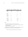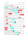
Download CURSA [1ex] Catalogue and Table Manipulation

SUN/190.11
Starlink Project
Starlink User Note 190.11
A.C. Davenhall
4th November 2001
c 2001 Council for the Central Laboratory of the Research Councils
Copyright CURSA
Catalogue and Table Manipulation
Applications
Version 6.4
User’s Manual
SUN/190.11 —Abstract
ii
Abstract
CURSA is a package of Starlink applications for manipulating astronomical catalogues and
similar tabular datasets. It provides facilities for: browsing or examining catalogues, selecting
subsets from a catalogue, sorting catalogues, copying catalogues, pairing two catalogues, converting catalogue coordinates between some celestial coordinate systems, plotting finding charts
and photometric calibration. Also, subsets can be extracted from a catalogue in a format suitable
for plotting using other Starlink packages, such as PONGO. CURSA can access catalogues held
in the popular FITS table format, the Tab-Separated Table (TST) format or the Small Text List
(STL) format. Catalogues in the STL and TST formats are simple ASCII text files. CURSA also
includes some facilities for accessing remote on-line catalogues via the Internet.
This manual describes how to use version 6.4 of CURSA. Its intended readership is users and
potential users of CURSA.
c 2001 Council for the Central Laboratory of the Research Councils
Copyright iii
SUN/190.11—Contents
Contents
1 Introduction
7
2 Obtaining copies of catalogues
7
3 Getting started
9
4 Terminology
4.1 Column attributes . . . . . . . . . . . . . . . . . . . . . . . . . . . . . . . . . . . . .
9
11
5 Null values
5.1 Processing null values . . . . . . . . . . . . . . . . . . . . . . . . . . . . . . . . . .
5.2 Displaying null values . . . . . . . . . . . . . . . . . . . . . . . . . . . . . . . . . .
12
12
13
6 Celestial coordinates
13
7 Target lists
14
8 Accessing catalogues
8.1 FITS tables . . . . . . . . . . . . . . . . . . . . . . . . . . . . . . . . . . . . . . . . .
8.2 TST . . . . . . . . . . . . . . . . . . . . . . . . . . . . . . . . . . . . . . . . . . . . .
8.3 STL . . . . . . . . . . . . . . . . . . . . . . . . . . . . . . . . . . . . . . . . . . . . .
15
16
16
17
9 Answering prompts in CURSA applications
17
10 Summary of applications
10.1 Copying textual information . .
10.2 Quiet mode . . . . . . . . . . .
10.3 Extra functionality . . . . . . .
10.4 Inter-operability with FTOOLS
10.5 Inter-operability with Starbase
.
.
.
.
.
17
18
19
20
20
21
11 Browsing and selecting with an X display
11.1 Statistics computed for individual columns . . . . . . . . . . . . . . . . . . . . . .
11.2 Restarting xcatview after a crash . . . . . . . . . . . . . . . . . . . . . . . . . . . .
21
22
25
12 Browsing and selecting from the command line
12.1 Running catview from a script . . . . . . . . . . . . . . . . . . . . . . . . . . . . . .
12.2 Continuation lines for long lists of columns and expressions . . . . . . . . . . . .
12.2.1 Examples . . . . . . . . . . . . . . . . . . . . . . . . . . . . . . . . . . . . .
25
30
30
32
13 Listing header details
33
14 Copying a catalogue
33
15 Sorting a catalogue
35
16 Selecting subsets from a catalogue
16.1 Running catselect . . . . . . . . . . . . . . . . . . . . . . . . . . . . . . . . . . . . .
16.2 Types of selections . . . . . . . . . . . . . . . . . . . . . . . . . . . . . . . . . . . .
36
37
38
.
.
.
.
.
.
.
.
.
.
.
.
.
.
.
.
.
.
.
.
.
.
.
.
.
.
.
.
.
.
.
.
.
.
.
.
.
.
.
.
.
.
.
.
.
.
.
.
.
.
.
.
.
.
.
.
.
.
.
.
.
.
.
.
.
.
.
.
.
.
.
.
.
.
.
.
.
.
.
.
.
.
.
.
.
.
.
.
.
.
.
.
.
.
.
.
.
.
.
.
.
.
.
.
.
.
.
.
.
.
.
.
.
.
.
.
.
.
.
.
.
.
.
.
.
.
.
.
.
.
.
.
.
.
.
.
.
.
.
.
SUN/190.11 —Contents
iv
17 Converting between celestial coordinate systems
17.1 Running catcoord . . . . . . . . . . . . . . . . . . . . . . . . . . . . . . . . . . . . .
40
41
18 Plotting finding charts
18.1 Suitable catalogues . . . . . . . . . . . . . . . . . .
18.1.1 Remote query . . . . . . . . . . . . . . . . .
18.1.2 Local copies . . . . . . . . . . . . . . . . . .
18.2 Running catchart . . . . . . . . . . . . . . . . . . .
18.3 Customising the plot . . . . . . . . . . . . . . . . .
18.3.1 Running catchartrn . . . . . . . . . . . . . .
18.3.2 Tutorial example graphics translation files
18.3.3 The graphics translation file . . . . . . . . .
18.4 Worked example . . . . . . . . . . . . . . . . . . .
42
43
43
43
44
45
46
47
50
54
.
.
.
.
.
.
.
.
.
.
.
.
.
.
.
.
.
.
.
.
.
.
.
.
.
.
.
.
.
.
.
.
.
.
.
.
.
.
.
.
.
.
.
.
.
.
.
.
.
.
.
.
.
.
.
.
.
.
.
.
.
.
.
.
.
.
.
.
.
.
.
.
.
.
.
.
.
.
.
.
.
.
.
.
.
.
.
.
.
.
.
.
.
.
.
.
.
.
.
.
.
.
.
.
.
.
.
.
.
.
.
.
.
.
.
.
.
.
.
.
.
.
.
.
.
.
.
.
.
.
.
.
.
.
.
.
.
.
.
.
.
.
.
.
.
.
.
.
.
.
.
.
.
.
.
.
.
.
.
.
.
.
19 Plotting with other packages
20 Pairing two catalogues
20.1 Requirements . . . . . . . . . . . . .
20.2 Running catpair . . . . . . . . . . . .
20.2.1 Special columns . . . . . . . .
20.2.2 Retaining specified columns .
20.2.3 Running from a script . . . .
20.3 Pairing criteria . . . . . . . . . . . . .
20.3.1 Cartesian coordinates . . . .
20.3.2 Celestial coordinates . . . . .
20.3.3 Cases for the critical distance
20.4 Rows in the output catalogue . . . .
20.5 Multiple matches . . . . . . . . . . .
20.6 Pairing algorithm . . . . . . . . . . .
56
.
.
.
.
.
.
.
.
.
.
.
.
57
58
59
62
62
63
63
65
65
65
66
67
69
.
.
.
.
.
.
.
.
.
70
70
72
72
74
74
75
78
79
79
22 Binning columns in a catalogue into a grid
22.1 Running catgrid . . . . . . . . . . . . . . . . . . . . . . . . . . . . . . . . . . . . . .
80
80
23 Importing CDS catalogues
23.1 Running catcdsin . . . . . . . . . . . . . . . . . . . . . . . . . . . . . . . . . . . . .
81
81
24 Importing regions of the HST GSC
82
.
.
.
.
.
.
.
.
.
.
.
.
.
.
.
.
.
.
.
.
.
.
.
.
21 Photometric calibration
21.1 Description . . . . . . . . . . . . . . . . .
21.2 Assembling the input catalogues . . . .
21.2.1 Standard star catalogue . . . . .
21.2.2 Programme object catalogue . .
21.3 Applications for photometric calibration
21.4 Running catphotomfit . . . . . . . . . .
21.5 Running catphotomtrn . . . . . . . . . .
21.6 Running catphotomlst . . . . . . . . . .
21.7 Calculating the air mass . . . . . . . . .
.
.
.
.
.
.
.
.
.
.
.
.
.
.
.
.
.
.
.
.
.
.
.
.
.
.
.
.
.
.
.
.
.
.
.
.
.
.
.
.
.
.
.
.
.
.
.
.
.
.
.
.
.
.
.
.
.
.
.
.
.
.
.
.
.
.
.
.
.
.
.
.
.
.
.
.
.
.
.
.
.
.
.
.
.
.
.
.
.
.
.
.
.
.
.
.
.
.
.
.
.
.
.
.
.
.
.
.
.
.
.
.
.
.
.
.
.
.
.
.
.
.
.
.
.
.
.
.
.
.
.
.
.
.
.
.
.
.
.
.
.
.
.
.
.
.
.
.
.
.
.
.
.
.
.
.
.
.
.
.
.
.
.
.
.
.
.
.
.
.
.
.
.
.
.
.
.
.
.
.
.
.
.
.
.
.
.
.
.
.
.
.
.
.
.
.
.
.
.
.
.
.
.
.
.
.
.
.
.
.
.
.
.
.
.
.
.
.
.
.
.
.
.
.
.
.
.
.
.
.
.
.
.
.
.
.
.
.
.
.
.
.
.
.
.
.
.
.
.
.
.
.
.
.
.
.
.
.
.
.
.
.
.
.
.
.
.
.
.
.
.
.
.
.
.
.
.
.
.
.
.
.
.
.
.
.
.
.
.
.
.
.
.
.
.
.
.
.
.
.
.
.
.
.
.
.
.
.
.
.
.
.
.
.
.
.
.
.
.
.
.
.
.
.
.
.
.
.
.
.
.
.
.
.
.
.
.
.
.
.
.
.
.
.
.
.
.
.
.
.
.
.
.
.
.
.
.
.
.
.
.
.
.
.
.
.
.
.
.
.
.
.
.
.
.
.
.
.
.
.
.
.
.
.
.
.
.
.
.
.
.
.
.
.
.
.
.
.
.
.
.
.
.
.
.
.
.
.
.
.
.
.
.
.
.
.
.
.
.
.
.
.
.
.
.
.
.
.
.
.
.
.
.
.
.
.
.
.
.
.
.
.
.
.
.
.
.
.
.
.
.
.
.
.
.
.
.
.
.
.
.
.
.
.
.
.
.
.
.
.
.
.
.
.
.
.
.
.
.
.
.
.
.
v
SUN/190.11 —Contents
25 Accessing remote catalogues
25.1 Running catremote . . . . . . . . . . . . . . . . . .
25.1.1 Listing the accessible catalogues . . . . . .
25.1.2 Querying a remote catalogue . . . . . . . .
25.1.3 Finding the coordinates of a named object .
25.2 Environment variables . . . . . . . . . . . . . . . .
25.3 Specifying the list of remote catalogues . . . . . .
25.3.1 Creating your own configuration file . . . .
25.4 How remote access works . . . . . . . . . . . . . .
25.5 Peculiarities and shortcomings . . . . . . . . . . .
25.6 Local or remote access? . . . . . . . . . . . . . . . .
.
.
.
.
.
.
.
.
.
.
83
84
85
85
87
87
88
88
89
89
90
.
.
.
.
.
.
91
91
91
92
92
92
95
B Storing and representing columns of angles
B.1 Angular format specifiers . . . . . . . . . . . . . . . . . . . . . . . . . . . . . . . .
95
96
A Expression syntax
A.1 Creating a new column . . . . . .
A.2 Defining a new selection . . . . .
A.3 Details of expressions . . . . . . .
A.4 Mathematical functions provided
A.5 Rules for expressions . . . . . . .
A.6 Operator precedence . . . . . . .
C Catalogue formats
C.1 FITS . . . . . . . . . . . . . .
C.1.1 Textual information .
C.2 TST . . . . . . . . . . . . . .
C.2.1 Textual information .
C.2.2 Null values . . . . .
C.3 STL . . . . . . . . . . . . . .
C.3.1 Textual information .
C.3.2 Null values . . . . .
.
.
.
.
.
.
.
.
.
.
.
.
.
.
.
.
.
.
.
.
.
.
.
.
.
.
.
.
.
.
.
.
.
.
.
.
.
.
.
.
.
.
.
.
.
.
.
.
.
.
.
.
.
.
.
.
.
.
.
.
.
.
.
.
.
.
.
.
.
.
.
.
.
.
.
.
.
.
.
.
.
.
.
.
.
.
.
.
.
.
.
.
.
.
.
.
.
.
.
.
.
.
.
.
.
.
.
.
.
.
.
.
.
.
.
.
.
.
.
.
.
.
.
.
.
.
.
.
.
.
.
.
.
.
.
.
.
.
.
.
.
.
.
.
.
.
.
.
.
.
.
.
.
.
.
.
.
.
.
.
.
.
.
.
.
.
.
.
.
.
.
.
.
.
.
.
.
.
.
.
.
.
.
.
.
.
.
.
.
.
.
.
.
.
.
.
.
.
.
.
.
.
.
.
.
.
.
.
.
.
.
.
.
.
.
.
.
.
.
.
.
.
.
.
.
.
.
.
.
.
.
.
.
.
.
.
.
.
.
.
.
.
.
.
.
.
.
.
.
.
.
.
.
.
.
.
.
.
.
.
.
.
.
.
.
.
.
.
.
.
.
.
.
.
.
.
.
.
.
.
.
.
.
.
.
.
.
.
.
.
.
.
.
.
.
.
.
.
.
.
.
.
.
.
.
.
.
.
.
.
.
.
.
.
.
.
.
.
.
.
.
.
.
.
.
.
.
.
.
.
.
.
.
.
.
.
.
.
.
.
.
.
.
.
.
.
.
.
.
.
.
.
.
.
.
.
.
.
.
.
.
.
.
.
.
.
.
.
.
.
.
.
.
.
.
.
.
.
.
.
.
.
.
.
.
.
.
.
.
.
.
.
.
.
.
.
.
.
.
.
.
.
.
.
.
.
.
.
.
.
.
.
.
.
.
.
.
.
.
.
.
.
.
.
.
.
.
.
.
.
.
.
.
.
.
.
.
.
.
.
.
.
.
.
.
.
.
.
.
.
.
.
.
.
.
.
.
.
.
.
.
.
.
.
.
.
.
.
.
.
.
.
.
.
.
.
.
.
.
.
.
.
.
.
.
.
.
.
.
.
.
.
.
.
.
.
.
.
.
.
.
.
.
.
.
.
.
.
.
.
.
.
.
.
.
.
.
.
.
.
.
.
.
.
.
.
.
.
.
.
.
.
.
.
.
.
.
.
.
.
.
.
.
.
.
.
.
.
.
.
.
.
.
.
.
.
.
.
.
.
.
.
.
.
.
.
.
.
.
.
.
.
.
.
.
.
.
.
.
.
102
102
103
103
104
104
104
105
105
D STL description tutorial
105
D.1 First example . . . . . . . . . . . . . . . . . . . . . . . . . . . . . . . . . . . . . . . 105
D.2 Second example . . . . . . . . . . . . . . . . . . . . . . . . . . . . . . . . . . . . . . 107
E STL description reference
E.1 Basics . . . . . . . . . . . . . . . . .
E.1.1 Continuation lines . . . . .
E.1.2 Strings . . . . . . . . . . . .
E.1.3 Comments . . . . . . . . . .
E.2 Columns . . . . . . . . . . . . . . .
E.2.1 Mandatory items . . . . . .
E.2.2 Optional items . . . . . . .
E.2.3 Storing sexagesimal angles
E.3 Parameters . . . . . . . . . . . . .
E.3.1 Mandatory items . . . . . .
E.3.2 Optional items . . . . . . .
.
.
.
.
.
.
.
.
.
.
.
.
.
.
.
.
.
.
.
.
.
.
.
.
.
.
.
.
.
.
.
.
.
.
.
.
.
.
.
.
.
.
.
.
.
.
.
.
.
.
.
.
.
.
.
.
.
.
.
.
.
.
.
.
.
.
.
.
.
.
.
.
.
.
.
.
.
.
.
.
.
.
.
.
.
.
.
.
.
.
.
.
.
.
.
.
.
.
.
.
.
.
.
.
.
.
.
.
.
.
.
.
.
.
.
.
.
.
.
.
.
.
.
.
.
.
.
.
.
.
.
.
.
.
.
.
.
.
.
.
.
.
.
.
.
.
.
.
.
.
.
.
.
.
.
.
.
.
.
.
.
.
.
.
.
.
.
.
.
.
.
.
.
.
.
.
.
.
.
.
.
.
.
.
.
.
.
.
.
.
.
.
.
.
.
.
.
.
.
.
.
.
.
.
.
.
.
.
.
.
.
.
.
.
.
.
.
.
.
.
.
.
.
.
.
.
.
.
.
.
.
.
.
.
.
.
.
.
.
.
.
.
.
.
.
.
.
.
.
.
.
.
.
.
.
.
.
.
.
.
.
.
.
.
.
.
.
.
.
.
.
.
.
.
.
.
.
.
.
.
.
.
.
.
.
.
.
.
.
.
.
.
.
.
.
.
.
109
109
110
111
111
111
111
111
113
116
116
118
SUN/190.11 —Contents
E.4 Directives
vi
. . . . . . . . . . . . . . . . . . . . . . . . . . . . . . . . . . . . . . . . . 118
F KAPPA format STL
119
F.1 Inter-operability with KAPPA . . . . . . . . . . . . . . . . . . . . . . . . . . . . . . 120
G Inter-operability with PISA
H Detailed description of applications
CATCDSIN . . . . . . . . . . . .
CATCHART . . . . . . . . . . .
CATCHARTRN . . . . . . . . .
CATCOORD . . . . . . . . . . .
CATCOPY . . . . . . . . . . . .
CATGRID . . . . . . . . . . . .
CATGSCIN . . . . . . . . . . . .
CATHEADER . . . . . . . . . .
CATPAIR . . . . . . . . . . . . .
CATPHOTOMFIT . . . . . . . .
CATPHOTOMLST . . . . . . .
CATPHOTOMTRN . . . . . . .
CATREMOTE . . . . . . . . . .
CATSELECT . . . . . . . . . . .
CATSORT . . . . . . . . . . . .
CATVIEW . . . . . . . . . . . .
References
120
.
.
.
.
.
.
.
.
.
.
.
.
.
.
.
.
.
.
.
.
.
.
.
.
.
.
.
.
.
.
.
.
.
.
.
.
.
.
.
.
.
.
.
.
.
.
.
.
.
.
.
.
.
.
.
.
.
.
.
.
.
.
.
.
.
.
.
.
.
.
.
.
.
.
.
.
.
.
.
.
.
.
.
.
.
.
.
.
.
.
.
.
.
.
.
.
.
.
.
.
.
.
.
.
.
.
.
.
.
.
.
.
.
.
.
.
.
.
.
.
.
.
.
.
.
.
.
.
.
.
.
.
.
.
.
.
.
.
.
.
.
.
.
.
.
.
.
.
.
.
.
.
.
.
.
.
.
.
.
.
.
.
.
.
.
.
.
.
.
.
.
.
.
.
.
.
.
.
.
.
.
.
.
.
.
.
.
.
.
.
.
.
.
.
.
.
.
.
.
.
.
.
.
.
.
.
.
.
.
.
.
.
.
.
.
.
.
.
.
.
.
.
.
.
.
.
.
.
.
.
.
.
.
.
.
.
.
.
.
.
.
.
.
.
.
.
.
.
.
.
.
.
.
.
.
.
.
.
.
.
.
.
.
.
.
.
.
.
.
.
.
.
.
.
.
.
.
.
.
.
.
.
.
.
.
.
.
.
.
.
.
.
.
.
.
.
.
.
.
.
.
.
.
.
.
.
.
.
.
.
.
.
.
.
.
.
.
.
.
.
.
.
.
.
.
.
.
.
.
.
.
.
.
.
.
.
.
.
.
.
.
.
.
.
.
.
.
.
.
.
.
.
.
.
.
.
.
.
.
.
.
.
.
.
.
.
.
.
.
.
.
.
.
.
.
.
.
.
.
.
.
.
.
.
.
.
.
.
.
.
.
.
.
.
.
.
.
.
.
.
.
.
.
.
.
.
.
.
.
.
.
.
.
.
.
.
.
.
.
.
.
.
.
.
.
.
.
.
.
.
.
.
.
.
.
.
.
.
.
.
.
.
.
.
.
.
.
.
.
.
.
.
.
.
.
.
.
.
.
.
.
.
.
.
121
122
124
126
128
131
134
136
138
140
143
146
147
149
152
159
161
166
vii
SUN/190.11—List of Figures
List of Figures
1
2
3
4
5
6
7
8
9
10
11
12
13
14
15
16
17
18
19
Example script for catview . . . . . . . . . . . . . . . . . . . . . . . . . . . . . .
Example STL format catalogue of polygon corners . . . . . . . . . . . . . . . . .
Simple graphics translation file . . . . . . . . . . . . . . . . . . . . . . . . . . . .
Star / galaxy graphics translation file . . . . . . . . . . . . . . . . . . . . . . . .
Procedure to produce a PONGO scatter-plot . . . . . . . . . . . . . . . . . . . .
Procedure to produce a PONGO Aitoff all-sky plot . . . . . . . . . . . . . . . . .
Two datasets for joining . . . . . . . . . . . . . . . . . . . . . . . . . . . . . . . .
An annotated example catpair script . . . . . . . . . . . . . . . . . . . . . . . .
Rows in paired catalogues . . . . . . . . . . . . . . . . . . . . . . . . . . . . . . .
A single primary object matches several secondary objects . . . . . . . . . . . .
A single secondary object is matched by several primary objects . . . . . . . . .
A crowded field with multiple matches of both primary and secondary objects
The index join . . . . . . . . . . . . . . . . . . . . . . . . . . . . . . . . . . . . . .
Example of a catalogue of photometric standard stars . . . . . . . . . . . . . . .
Example of a catalogue of photometric programme objects . . . . . . . . . . . .
Example output from catphotomfit . . . . . . . . . . . . . . . . . . . . . . . . .
A simple STL description file . . . . . . . . . . . . . . . . . . . . . . . . . . . . .
A more complicated STL description file . . . . . . . . . . . . . . . . . . . . . .
Example STL format catalogue with complex sexagesimal angles . . . . . . . .
. 31
. 39
. 48
. 49
. 56
. 57
. 58
. 64
. 66
. 68
. 68
. 68
. 69
. 73
. 75
. 77
. 106
. 108
. 117
1
SUN/190.11 —List of Figures
CURSA Quick Reference
To set up for using CURSA type:
cursa
Applications
xcatview
browse and generate selections from a catalogue (X-windows, easy-to-use),
catview
browse and generate selections from a catalogue (command line),
catselect
select a subset from a catalogue,
catcoord
convert between celestial coordinate systems,
catchart
plot a finding chart,
catchartrn
set up ready for plotting a finding chart,
catheader
list various header information for a catalogue,
catcopy
copy a catalogue,
catsort
sort a catalogue,
catpair
pair two catalogues,
catgrid
bin one, two or three columns into a histogram, image or data cube,
catphotomfit
define photometric transformation coefficients,
catphotomtrn
apply photometric transformation coefficients to programme objects,
catphotomlst
list photometric transformation coefficients,
catcdsin
convert a CDS text catalogue to STL format,
catgscin
convert a region in the HST Guide Star Catalog to a more convenient format,
catremote
access remote on-line catalogues.
Catalogue formats
FITS tables (file types: .FIT .fit .FITS .fits .GSC .gsc). Binary and ASCII FITS tables.
TST (file types: .TAB .tab). The Tab-Separated Table format used by GAIA.
STL (file types: .TXT .txt). The Small Text List format.
Expressions
arithmetic operators: + - * / **
relational operators: .EQ. .NE. .GE. .GT. .LE. .LT. == /= >= > <= <
logical (boolean) operators: .AND. .OR. .NOT. & | #
brackets: use brackets, ‘(’, ‘)’, as appropriate,
sexagesimal values: use a colon (‘:’) to separate hours/degrees, minutes and seconds. Unsigned
SUN/190.11 —List of Figures
2
values are interpreted as hours; values in degrees must always have a sign (‘+’ or ‘-’). Sexagesimal values are converted to radians prior to evaluating the expression.
great circle distance: GREAT(α1 , δ1 ,α2 , δ2 )
position angle of point (α2 , δ2 ) from point (α1 , δ1 ): PANGLE(α1 , δ1 ,α2 , δ2 )
3
SUN/190.11 —List of Figures
CURSA home page and on-line documentation
A ‘home page’ giving useful information about CURSA is available via the World Wide Web. Its
URL is:
http://www.starlink.ac.uk/cursa/
An on-line version of SUN/190 (this manual) is also available via the World Wide Web. On
Starlink systems type:
% showme sun190
Otherwise access URL:
http://www.starlink.ac.uk/docs/sun190.htx/sun190.html
Assistance and further information
If you are experiencing difficulties using CURSA then in the first instance you should probably
seek advice and assistance from your local site manager. Bug reports should be sent to username:
[email protected]
Bug reports should always be sent to username [email protected]. However, you are
welcome to contact me directly for advice and assistance. Suggestions for enhancements and
improvements to CURSA are also welcome. Details of how to contact me are given below.
Clive Davenhall
Postal address: Institute for Astronomy, Royal Observatory, Blackford Hill, Edinburgh,
EH9 3HJ, United Kingdom.
Electronic mail: [email protected]
Fax:
from within the United Kingdom:
from overseas:
0131-668-8416
+44-131-668-8416
SUN/190.11 —List of Figures
4
Acknowledgments
CURSA is far from being all my own work. Clive Page, Rodney Warren-Smith and Alan Wood
have all been involved in aspects of its development. Indeed, Clive Page wrote the expression
parser which CURSA uses, and Appendix A is based on documentation which he supplied.
Malcolm Currie and Anne Sansom tested an early version of xcatview and suggested several
significant improvements. Numerous other people have made useful contributions.
I am grateful to everyone who has contributed time and expertise.
Clive Davenhall
Department of Physics and Astronomy, University of Leicester
Saint Indract’s Day 1995
Various items of external software have been introduced into version 3.1 of CURSA which it
is a pleasure to acknowledge. catremote accesses remote on-line catalogues using the catlib
library developed by Allan Brighton, Miguel Albrecht and colleagues at the European Southern
Observatory. Patrick Wallace gave useful advice and assistance during the development of
catcoord and this application uses his SLA library to convert between celestial coordinate
systems. catchart uses Tim Pearson’s PGPLOT to produce its plots. Last, but not least, FITS
tables continue to be accessed using Bill Pence’s invaluable FITSIO library. I am also grateful to
the numerous people who have commented on, and suggested improvements to, CURSA.
Clive Davenhall
Institute for Astronomy, University of Edinburgh
Saint Médard’s Day 1997
I am grateful to John Lucey for useful discussions about photometric calibration and for kindly
providing the data used in the example catalogue of observations of photometric standard stars.
Peter Draper gave helpful comments on the section of the manual describing the photometric
calibration.
Clive Davenhall
Institute for Astronomy, University of Edinburgh
Saint Aed’s Day 1997
5
SUN/190.11 —List of Figures
Revision history
(1) 8th May 1995: Original draft (ACD).
(2) 10th October 1995: Version 1 (ACD).
(3) 11th April 1996: Version 2. Modified so that the Latex source could be used to create an
HTML as well as a paper version (ACD).
(4) 31st January 1997: Version 3. Modified for release 2.1 of the CURSA package. The major
changes were the addition of the Small Text List (STL) format and the new application
catselect (ACD).
(5) 8th June 1997: Version 4. Modified for release 3.1 of the CURSA package. The major changes were the new applications catcoord, catchart, catchartrn and catremote
(ACD).
(6) 10th November 1997: Version 5. Modified for release 4.1 of the CURSA package. The
major changes were the new applications for photometric calibration: catphotomfit,
catphotomtrn and catphotomlst (ACD).
(7) 13th December 1998: Version 6. Modified for release 5.1 of the CURSA package. The
major changes were the new application catcdsin and additional formats for reading
sexagesimal angles from fixed-format STL catalogues (ACD).
(8) 29th November 1999: Version 7. Modified for release 6.1 of the CURSA package. The major
changes were the addition of the Tab-Separated Table (TST) format, the new application
catgrid and options for plotting scatter-plots and histograms in xcatview (ACD).
(9) 25th July 2000: Version 8. Modified for release 6.2 of the CURSA package. Version 6.2
contains no major enhancements, just some minor improvements and bug fixes. The
main changes to the document are the removal of the description of the Tab-Separated
Table (TST) format, which has been moved to SSN/75 and the inclusion of an additional
appendix in the hyper-text version which gives descriptions of individual applications
(ACD).
(10) 14th May 2001: Version 9. Modified for release 6.3 of the CURSA package. Version 6.3
contains no major changes, but rather a number of enhancements and bug fixes. There are
improvements to the applications catcopy and catchart. The facilities to access remote
catalogues via the Internet have been completely re-worked. A ‘quiet mode’ has been
added to most of the applications. Support for the little-used CHI/HDS catalogue format
has been removed.
(11) 4th November 2001: Version 10. Modified for release 6.4 of the CURSA package. Version
6.4 contains no major enhancements. Application catheader has been re-worked and now
offers various options and more convenient output. A bug in xcatview has been fixed.
SUN/190.11 —List of Figures
6
7
1
SUN/190.11 —Obtaining copies of catalogues
Introduction
CURSA1 (Catalogue Utilities for Reporting, Selecting and Arithmetic) is a package of Starlink
applications for manipulating astronomical catalogues and similar tabular datasets. This manual
describes version 6.4 of CURSA. Though CURSA is primarily intended for use with astronomical
catalogues it can be used equally well with other tabular data, such as a table of private
astronomical results, or, indeed, data which are entirely non-astronomical, provided that they
are in an appropriate format.
The facilities provided by CURSA include: browsing or examining catalogues, selecting subsets
from catalogues, sorting catalogues, copying catalogues, pairing two catalogues, converting
catalogue coordinates between some celestial coordinate systems, plotting finding charts and
photometric calibration. Also, subsets can be extracted from a catalogue in a format suitable for
plotting using other Starlink packages, such as PONGO.
CURSA can access catalogues held in either the popular FITS table format, the Tab-Separated
Table (TST) format or the Small Text List (STL) format. Both ASCII and binary FITS tables can be
read, though only binary FITS tables can be written. Catalogues in the STL and TST formats are
simple ASCII text files which can be created with a text editor. Unlike the other formats which
CURSA can access, the STL format is specific to CURSA. Nonetheless, the STL format exists in
order to allow easy access to both private tables and versions of standard catalogues held as
text files. It is usually straightforward to create an STL catalogue from a text file containing a
private list or catalogue. CURSA includes a facility for automatically converting text versions
of catalogues obtained from the Centre de Données astronomiques de Strasbourg (CDS) into
the STL format. CURSA also has some facilities for accessing remote on-line catalogues via the
Internet.
CURSA is available on all the variants of Unix currently supported by Starlink. The following
section briefly describes some sources of catalogues in suitable formats. Subsequent sections
introduce some general information about CURSA and the later sections describe the individual
applications. Two tutorial examples (‘recipes’ in the jargon of cookbooks) of using CURSA are
included in SC/6: The CCD Photometric Calibration Cookbook[22].
2
Obtaining copies of catalogues
The FITS table format is a popular and widely used format for distributing astronomical catalogues. Several CD-ROMs contain catalogues in this format. Some of the more generally useful
ones are:
• Selected Astronomical Catalogs volumes I, II, III and IV, produced by the US Astronomical
Data Center (ADC) at the NASA Goddard Space Flight Center,
• HST Guide Star Catalog, produced by the NASA Space Telescope Science Institute (see
Section 24, below),
1 Cursa
is the common name for β Eridanus. It is of Arabic origin and derives from an abbreviation of the name of
an asterism involving λ, β and ψ Eri and τ Ori: ‘the Foremost Footstool of Orion’. These details come from a Short
Guide to Modern Star Names and Their Derivations by P. Kunitzsch and T. Smart[18].
SUN/190.11 —Obtaining copies of catalogues
8
• several of the Einstein Observatory CD-ROMs.
In particular the four volumes of Selected Astronomical Catalogs are an extremely useful collection
of widely used catalogues. Also, the Centre de Données astronomiques de Strasbourg (CDS)
and the US Astronomical Data Center now make many of the catalogues in their extensive
collections available on-line. Briefly, the CDS and ADC may be contacted as follows.
CDS URL: http://cdsweb.u-strasbg.fr/CDS.html
Anonymous ftp site: cdsarc.u-strasbg.fr, directory: /pub/cats
Electronic mail: [email protected]
Postal address: Centre de Données astronomiques de Strasbourg, Observatoire de Strasbourg, 11, rue de l’Université, 67000 Strasbourg, France.
ADC URL: http://adc.gsfc.nasa.gov/
Anonymous ftp site: adc.gsfc.nasa.gov, directory: /pub/adc/archives
Electronic mail: [email protected]
Postal address: World Data Center A for Rockets and Satellites, NASA, Goddard Space
Flight Center, Code 633, Greenbelt, Maryland 20771, USA.
In the case of the CDS catalogues can usually be retrieved as either FITS files or simple text
files. It is usually preferable to retrieve the catalogues as text files because they can then be
automatically reformatted into CURSA STL format catalogues (see Section 23) which properly
interpret their coordinates, thus allowing full use of CURSA’s facilities for manipulating and
displaying angles (see Section 6 and Appendix B).
Further details of the CD-ROMs and the data centres may be found in the CURSA ‘home page’
(see page 3 for the URL) and in SUN/162[7], though the latter is now somewhat out of date.
An additional small collection of catalogues which have had their celestial coordinates reformatted to take full advantage of CURSA’s facilities for manipulating and displaying angles (see
Section 6 and Appendix B) is available by anonymous ftp. The details are as follows.
Anonymous ftp to:
ftp.roe.ac.uk
Directory:
/pub/acd/catalogues
Remember to reply anonymous when prompted for a username and to give your e-mail address
as the password. Retrieve file 0CONTENTS.LIS for a list of the catalogues available. If you
encounter difficulty using ftp then contact your site manager in the first instance. The list of
catalogues is also available from the CURSA home page.
CURSA includes a facility which provides some limited access to remote catalogues held on-line
at various astronomical data centres and archives around the world. You can select a subset from
one of these catalogues and save it as a CURSA Tab-Separated Table (TST) format catalogue
which can then be input to the other CURSA applications. This facility is available as part of
xcatview (see Section 11) and as application catremote (see Section 25).
In the past Starlink provided the SCAR (Starlink Catalogue Access and Reporting) system for
manipulating astronomical catalogues on its VAX/VMS service. SCAR had its own unique
9
SUN/190.11 —Terminology
format for storing catalogues. It is possible to convert SCAR catalogues to FITS tables and make
them accessible to CURSA. If you have any SCAR catalogues (either public catalogues from the
standard collection or private catalogues) which you would like converted then please contact
me in the first instance (see page 3 for details).
3
Getting started
CURSA is an optional Starlink software item. Before proceeding you should check with your
local site manager whether it is installed at your site, and if not attempt to persuade him to
install it. If CURSA is installed at your site the following directory should exist:
/star/bin/cursa
The procedure to set up for using CURSA is the same on all the variants of Unix supported by
Starlink. Simply type:
% cursa
The following message should appear:
CURSA commands are now available -- (Version 6.3)
If it does not, then the probable cause is that CURSA is not installed correctly at your site; check
with your local site manager.
You do not need any special quotas or privileges to use CURSA. However, obviously, you need
enough disk space to accommodate any catalogues that you might use and any output files that
you might create.
4
Terminology
An astronomical catalogue is basically a table of values, consisting of the measurements of the
same property for a set of objects, together with the auxiliary information necessary to describe
this table. There are several different terminologies for describing the elements of such tables.
For simplicity, in CURSA a terminology which corresponds loosely to that used intuitively for
the paper versions of astronomical catalogues is used:
row the values for all the properties associated with some particular object,
column the value of a single property for all the objects in a catalogue,
field the value of a single property for a single object (that is, the intersection of a row and a
column).
SUN/190.11 —Terminology
10
CURSA
Fortran
Relational Database
table
file
relation
row
record
tuple
column
field
attribute
field
data item, field
component
format
format
schema
number of columns
number of fields
arity, degree
number of rows
number of records
cardinality
Table 1: Alternative terminologies for the components of tables
Some of the other terminologies are shown for comparison in Table 12 .
In CURSA each catalogue can contain only one table and the two terms can usually be used
interchangeably without introducing any ambiguity. However, where it is necessary to differentiate between the two sorts of entities, table is used to denote the simple matrix of rows
and columns and catalogue is used to denote the combination of a table and its associated
auxiliary information. (Note, however, that this usage implies nothing about the contents of
the catalogue; it may contain a published astronomical catalogue, a set of private astronomical
results or, indeed, data which are entirely non-astronomical.)
A CURSA catalogue which contains celestial coordinates in a restricted format which CURSA
can interpret is called a target list. The applications which convert between celestial coordinates
and plot finding charts operate on target lists. Target lists are described in Section 7.
Columns may either be scalars in which case each field comprises a single datum, or vectors,
one-dimensional arrays where each field comprises a one-dimensional array of values.
Columns have a number of attributes, such as their name, data type and units. A column’s
attributes hold all the details which define its characteristics. The more important column
attributes are described in Section 4.1, below.
Catalogues can also contain auxiliary information which applies to the entire catalogue. CURSA
recognises two types of auxiliary information: parameters and textual information. A parameter is a single datum, such as the epoch or equinox of celestial coordinates stored in a catalogue.
CURSA parameters are similar to FITS keywords (in fact, CURSA interprets named keywords
in a FITS table as parameters). Parameters have attributes similar to columns.
Textual information is information, usually descriptive, associated with the catalogue and
intended to be read by a human. For a FITS table the textual information is basically the contents
of any ‘COMMENTS’ and ‘HISTORY’ keywords3 .
In the jargon of relational database systems auxiliary information is often called metadata. In
the context of CURSA the metadata for a catalogue comprises the details of the columns (name,
data type, units, etc.), the parameters and the textual information.
2 This
table is adapted from Database Systems in Science and Engineering by J.R. Rumble and F.J. Smith[24], p158.
statement is something of an over-simplification. See Appendix C for a complete description of the way
that FITS headers are interpreted as textual information.
3 This
11
4.1
SUN/190.11 —Terminology
Column attributes
In order to use CURSA you do not need to know the details of all the attributes of a column, but
there are a few which you will probably encounter. These attributes are listed in Table 2 and are
described briefly below.
Attribute
Comments
NAME
Name of the column
DTYPE
Data type
DIMS
Dimensionality: scalar or vector
SIZE
Size (number of elements) of a vector
UNITS
Units of the column
EXFMT
External display format
COMM
Comments describing the column
Table 2: Attributes of columns
NAME The name of the column. The rules for column names are as follows.
• The name must be unique within the totality of parameters and columns for the catalogue.
This condition is necessary in order that a component (parameter or column) may be
identified unambiguously when its name is used in an expression (see Appendix A).
• A name may comprise up to fifteen characters. This value is chosen for consistency with
HDS and is adequate for FITS tables.
• The name can contain only: upper or lower case alphabetic characters (a-z, A-Z), numeric characters (0-9) and the underscore character (‘_’). Note that lower case alphabetic
characters must be allowed in order to access existing FITS tables. However, corresponding
upper and lower case characters are considered to be equivalent. Thus, for example, the names:
HD_NUMBER, HD_Number and hd_number would all refer to the same column.
• The first character must be a letter.
DTYPE The data type of values held in the column. CURSA supports the standard data
types of Fortran 77 (apart from the COMPLEX data types) and also signed one and two byte
INTEGERs.
DIMS
The dimensionality of the column: scalar or a vector.
SIZE If the column is a vector this attribute contains the number of elements in the vector. If
the column is a scalar it is set to one.
SUN/190.11 —Null values
12
UNITS The units in which values stored in the column are expressed. The UNITS attribute
is used to identify, and control the appearance of, columns of angles (see Appendix B). Apart
from this exception the units are treated purely as comments and no attempts are made to
automatically propagate and convert units in calculations and selections.
EXFMT The format used to represent a field extracted from a column for external display by
xcatview (see section 11) or catview (see section 12). The external format specifier should be a
valid Fortran 77 format specifier for the data type of the column.
COMM
5
Explanatory comments describing the column.
Null values
CURSA supports null values in catalogues. Null values are used to represent a field for which
no actual value is available. Null values can arise in several ways. They may be present
in a catalogue when it is read by CURSA. An example might be a catalogue of multi-colour
photometry for a set of stars where measures for some colours were missing for some of the
stars. Null values would be used to represent the missing values. Alternatively, they might arise
where an expression is being used to compute a new column and evaluation of the expression for
the current row results in a ‘÷ by zero’ error. No valid value will be available for the expression,
so a null value will be substituted.
Throughout CURSA null values have the single, simple meaning that ‘no value is available for
this datum’. It is possible to invent schemes where a set of null values are supported, each with
a subtly different gradation of meaning. However, CURSA does not support such schemes.
5.1
Processing null values
You do not need to know all the details of how CURSA manipulates null values internally.
However, the following points may be useful.
• When a value for a new column is computed from an algebraic expression in which one of
the input fields is null, then the result is also null. For example, if the new column was
being computed for the expression ‘x + y’ then the result would be null if either x or y (or
both) were null. The generation of a null in this fashion is not considered an error and no
message or warning is reported.
• When a relational expression is being used to generate a selection then rows for fields
with null values occurring in the expression do not satisfy the expression. For example,
if the selection was defined by ‘x > 2.0’ then rows where x is null would not satisfy the
expression.
• The function NULL is available to determine whether a field is null or not. For example, to
select the rows for which column x is not null the following expression would be used:
‘.NOT. NULL(x)’.
13
5.2
SUN/190.11 —Celestial coordinates
Displaying null values
When null values are displayed by xcatview (see Section 11) or catview (see Section 12) they
will normally be represented by the string ‘<null>’. However, if there is insufficient space to
display them in this way they will be represented by the single character ‘?’.
6
Celestial coordinates
Most astronomical catalogues contain columns of celestial coordinates of some sort: usually
Right Ascension and Declination for some equinox and epoch, or perhaps Galactic or ecliptic
coordinates. The storage, manipulation and presentation for display of celestial coordinates in
the computer-readable version of astronomical catalogues is something of a vexed topic which
has caused a deal of confusion and difficulty, much of it, in principle, unnecessary.
For preexisting catalogues, such as those described in Section 2, the format of the celestial
coordinates will already be fixed and CURSA will simply display the columns in whatever way
is possible. For example, many catalogues contain the hours, or degrees, minutes and seconds
which comprise a coordinate as separate columns; a form which is singularly inconvenient for
further processing. However, CURSA has some special facilities for processing and displaying
coordinates, and catalogues that have been specifically prepared for CURSA can take advantage
of these.
CURSA can store columns of coordinates as radians but automatically present them as sexagesimal hours or degrees when they are listed by the browsing applications xcatview (see Section 11)
or catview (see Section 12). The advantages of this approach are that internally within CURSA
the coordinates remain in radians, which is the most convenient form for computations, but they
are presented to the user, and he interacts with them, as sexagesimal hours or degrees, which is
the way that he naturally thinks about them.
Also, it is possible within xcatview or catview to interactively alter the precise way that a
coordinate is formatted for display. These facilities are described in detail in Appendix B.
Similarly, while displaying coordinates in units of hours or degrees formatted as sexagesimal
values is usually the required behaviour, occasionally you may want to display angles as simple
decimal numbers expressed in radians (as they are represented internally). Both xcatview and
catview provide this facility.
CURSA application catgscin (see Section 24) reformats coordinates in regions of the HST
Guide Star Catalog to a format which is fully compatible with CURSA. Similarly, catremote
(see Section 25), the application for extracting subsets from remote on-line catalogues, returns
coordinates which are fully compatible. Also, catcdsin (see Section 23) will usually reformat
the text versions of CDS catalogues into STL format catalogues containing CURSA-compatible
coordinates. Finally, the CURSA ‘home page’ (see page 3 for the URL) contains a list of catalogues
which have been converted to have coordinates which are fully compatible with CURSA.
SUN/190.11 —Target lists
7
14
Target lists
A target list is a catalogue which contains celestial coordinates in a restricted format which
CURSA can interpret. The applications for converting between celestial coordinate systems,
catcoord (see Section 17) and plotting finding charts, catchart (see Section 18) read target
lists. The applications for importing a region from the HST Guide Star Catalog, catgscin (see
Section 24) and extracting a subset from a remote catalogue, catremote (see Section 25) produce
target lists. Similarly, the catalogues generated with catcdsin (see Section 23) from the text
version of CDS catalogues are usually target lists. Though a target list places restrictions on the
names and units of the celestial coordinates, the catalogue itself can be in any of the formats
supported by CURSA: FITS table, TST or STL (see Appendix C).
A target list must contain columns of Right Ascension and Declination, for some equinox and
epoch, called respectively RA and DEC. These coordinates must be stored in radians in a format
which CURSA can interpret (see Section 6, above and Appendix B).
Additional optional columns allow the proper motion, parallax and radial velocity to be specified.
These quantities are used for accurate conversions between celestial coordinate systems. All
the columns which can be used to specify coordinates in a target list are listed in Table 3. The
columns marked with a bullet (‘•’) in the ‘Mandatory’ column must be present. The other
columns are optional. However, if they are present they must be used as described. The
names of the columns are chosen to be consistent with the recommendations of the CDS (see
Astronomical Catalogues at CDS: Adopted Standards by F. Ochsenbein[21], p14).
Description
Name
Units
Mandatory?
Right Ascension
RA
Radians
•
Declination
DEC
Radians
•
Annual proper motion in Right Ascension
PMRA
Radians
Annual Proper motion in Declination
PMDE
Radians
Parallax
PLX
Radians
Radial velocity
RV
Km/sec
Table 3: Columns defining celestial coordinates in a target list
The proper motions are specified per year rather than per century. Also the proper motion in
Right Ascension is simply the rate of change of Right Ascension, α̇ (leading to large values for
stars close to the poles), not the angle on the sky, α̇ cos δ. The latter quantity is tabulated in some
catalogues. Similarly some catalogues give the proper motion as a position angle and size. In
both these cases the tabulated values must be converted to the required form before they can be
used in a target list.
The usual astronomical sign convention for radial velocity is used: objects which are receding
should have a positive radial velocity.
A target list can also contain two optional parameters: EQUINOX and EPOCH. These parameters
15
SUN/190.11 —Accessing catalogues
respectively contain the equinox and epoch of the coordinates. Both parameters are of data type
CHARACTER.
The value of both parameters is a Besselian or Julian epoch4 expressed in years. The numeric
value may optionally be preceded by a letter ‘B’ or ‘J’ to indicate a Besselian or Julian epoch
respectively. If this preceding letter is omitted then values before 1984.0 are assumed to be
Besselian and subsequent values to be Julian. This behaviour is consistent with the relevant IAU
recommendations. Table 4 lists some examples of valid equinoxes and epochs.
Example
Notes
B1950
often used in older catalogues
J2000
often used in modern catalogues
B1975
1992.37
interpreted as J1992.37 (because after 1984.0)
1943
interpreted as B1943.0 (because before 1984.0)
B1987
‘B’ is necessary here (because after 1984.0)
Table 4: Example equinoxes and epochs
An example of a simple target list is available as file /star/share/cursa/simple.TXT. In
this target list the coordinates simply comprise Right Ascension and Declination. A more
complicated example where the coordinates include proper motions etc. is available as file
/star/share/cursa/propmotn.TXT. Note that though CURSA must interpret the columns of
proper motions etc. as having units of radians they can be tabulated in an STL format catalogue
in seconds of arc by using the TBLFMT option in the column definitions, as in this example. This
option will often be convenient when creating target lists.
8
Accessing catalogues
Most of the CURSA applications prompt you to enter the name of at least one catalogue. You
should reply with the name of the file containing the catalogue. The file name of a CURSA
catalogue comprises the ‘catalogue name’ followed by the ‘file type’, for example:
perseus.FIT
where ‘perseus’ is the catalogue name and ‘.FIT’ the file type. The catalogue name is restricted
to contain only: upper or lower case alphabetic characters (a-z, A-Z), numeric characters (0-9)
and the underscore character (‘_’). The file name may optionally be preceded by a directory
specification.
CURSA uses the ‘file type’ of the file name to determine the format of the catalogue (FITS table,
TST or STL) and therefore the file name must end in the appropriate file type. The file types for
the three catalogue formats are:
4 In
this context an epoch is simply an instant of time.
SUN/190.11 —Accessing catalogues
FITS table:
.FIT .fit .FITS .fits .GSC .gsc
TST:
.TAB .tab
STL:
.TXT .txt
16
The .GSC and .gsc file types for FITS tables are provided in order to allow regions of the HST
Guide Star Catalog to be accessed easily. Other FITS tables obtained from an external source, such
as those mentioned in Section 2, may have a different file type. They must be renamed (with the
Unix command mv) to have a recognised file type before they can be accessed with CURSA.
A few additional details which are specific to the individual catalogue formats are described
below. The peculiarities and limitations of the three catalogue formats are described in full in
Appendix C.
8.1
FITS tables
(File types: .FIT .fit .FITS .fits .GSC .gsc). Mixed capitalisations, such as .Fit, are also
supported. To access a FITS table in the current directory you need only supply the file name.
To access a FITS table in another directory you should precede the file name with an absolute or
relative directory specification5 .
Usually the table component of a FITS file occurs in the first FITS extension to the file. When
reading an existing FITS file CURSA will look for a table in the first extension. In cases where
the table is located in an extension other than the first you can specify the required extension
by giving its number inside curly brackets after the name of the file. For example, if the table
occurred in the third extension of a FITS file called perseus.FIT you would specify:
perseus.FIT{3}
The closing curly bracket is optional. When CURSA writes FITS tables the table is always written
to the first extension.
8.2
TST
(File types: .TAB .tab). Mixed capitalisations, such as .Tab, are also supported. To access a TST
(Tab-Separated Table) format catalogue in the current directory you need only supply the file
name. To access a TST catalogue in another directory you should precede the file name with an
absolute or relative directory specification.
5
Of course, you can precede the name of a catalogue in the current directory with a directory specification if you
want to, but there is no point in doing so.
17
SUN/190.11 —Summary of applications
8.3
STL
(File types: .TXT .txt). Mixed capitalisations, such as .Txt, are also supported. To access an
STL (Small Text List) format catalogue in the current directory you need only supply the file
name. To access an STL catalogue in another directory you should precede the file name with an
absolute or relative directory specification.
An input STL catalogue may be in either the standard form or the KAPPA variant form (see
Appendix F). By default CURSA writes standard STLs. It can be made to write a KAPPA variant
STL by appending ‘KAPPA’ inside curly brackets after the name of the file. For example, to write
a KAPPA variant STL called perseus.TXT you would specify:
perseus.TXT{KAPPA}
‘KAPPA’ can be abbreviated down to just ‘K’ and can be given in either case. Also the closing curly
bracket is optional.
9
Answering prompts in CURSA applications
Clearly you will usually reply to a prompt from a CURSA application by entering a suitable
value. However, as usual for Starlink applications, the following special replies may also be
entered:
? display one line of help information about the prompt, and then re-prompt,
! a value is not available to answer the prompt. The application will take appropriate action;
in CURSA it will usually abort,
!! abort the application6 .
Note that these special replies are not available in catcdsin (see Section 23) and catremote (see
Section 25).
10
Summary of applications
CURSA contains the following applications.
xcatview browse and generate selections from a catalogue (easy-to-use X-windows version
with a graphical user interface; see Section 11),
catview browse and generate selections from a catalogue (command line version; see Section 12),
6 Of
course the application may also be aborted by typing ‘<Control-C>’. Typing ‘<Control-C>’ is less likely to
tidy up properly any files which are open, though this is unlikely to be important in practice.
SUN/190.11 —Summary of applications
18
catheader list various header information for a catalogue (see Section 13),
catcopy copy a catalogue (see Section 14),
catsort sort a catalogue (see Section 15),
catselect select a subset from a catalogue and save it as a new catalogue (see Section 16),
catcoord convert catalogue coordinates between celestial coordinate systems (see Section 17),
catchart plot a basic finding chart from a target list (see Section 18),
catchartrn customise a target list for prior to plotting it as a finding chart (see Section 18),
catpair pair two catalogues (see Section 20),
catphotomfit define photometric transformation coefficients using observations of standard
stars (see Section 21),
catphotomtrn apply photometric transformation coefficients to programme objects (see Section 21),
catphotomlst list photometric transformation coefficients (see Section 21),
catgrid bin one, two or three columns from a catalogue into, respectively, a histogram, image
or data cube (see Section 22),
catcdsin convert the text file version of a CDS catalogue to the CURSA STL format (see
Section 23),
catgscin convert a region in the HST Guide Star Catalog to a more convenient format (see
Section 24),
catremote extract a subset from a remote on-line catalogue (see Section 25).
To run any of the applications you simply type its name and answer the ensuing prompts (or, in
the case of xcatview dialogue boxes).
xcatview and catview provide essentially the same functionality. However, xcatview is much
easier to use and is strongly recommended over catview for casual, interactive examination of a
catalogue. It does, however, have to be run from a terminal (or workstation console) capable of
supporting X-windows output. The only circumstances where catview is likely to be preferable
are if you have a terminal which does not support X output or you are performing repetitive
‘batch’ type operations from a script.
10.1
Copying textual information
The applications which create a new catalogue from an existing one (catcopy, catsort,
catselect, catcoord, catchartrn, catphotomtrn and catgscin) all have a uniform option to
control the amount of textual information that they write to the new catalogue.
By default the textual information for the new catalogue is a copy of the textual information
for the original catalogue (which is usually what is required). However, options are available
to either copy all the details of the original catalogue (including the column and parameter
19
SUN/190.11 —Summary of applications
definitions) as textual information for the new catalogue or to copy no textual information to
the new catalogue.
These options are invoked by specifying an extra item on the command line when the application
is invoked. For example, for catcopy:
• to copy just the textual information from the original catalogue simply give the command
name:
catcopy
• to copy the entire description of the input catalogue as textual information in the output
catalogue:
catcopy text=all
• to copy no textual information to the output catalogue:
catcopy
text=none
The other applications include exactly the same way option. There must be one or more spaces
between the application name and the ‘text=’ item.
10.2
Quiet mode
Most of the applications have a ‘quiet mode’ in which they issue fewer informational and
warning messages. The exceptions are catcdsin and catremote, which are Perl scripts rather
than conventional applications. The quiet mode suppresses only some informational and
warning messages; it does not affect error messages. All the applications which support the
quiet mode use the same mechanism to control it. By default the applications are in a ‘verbose’
mode in which they issue informational and warning messages. To switch to quiet mode an
additional option is specified when invoking any of the applications which support it, for
example:
catcopy
quiet=true
The quiet mode will now remain in effect, not just for the one invocation of catcopy, but for all
subsequent invocations of all the applications that support the quiet mode. To revert to verbose
mode type, for example:
catchart
quiet=false
The quiet mode can also be set as one of the configuration options of xcatview (see Section 11). Finally, I advise you to use the quiet mode with caution; it is usually better to see the informational
and warning messages.
SUN/190.11 —Summary of applications
10.3
20
Extra functionality
CURSA can inter-operate with a number of other packages. These packages provide additional
functionality which is not available in CURSA. Perhaps the most extensive and useful is FTOOLS,
which is briefly described in Section 10.4, below. Another useful external package is Starbase,
which is briefly described in Section 10.5, below.
The image display and analysis tool GAIA[12] reads and writes catalogues in the TST format.
Thus, catalogues in this format can be exchanged between CURSA and GAIA. Some limited
inter-operability is possible between CURSA and the image processing package KAPPA[5] (see
Appendix F) and the image analysis package PISA[13] (see Appendix G).
Finally, CURSA is augmented by the CAT Fortran 77 subroutine library for manipulating
catalogues and tables. Using CAT it is straightforward to write your own programs to perform
specialised tasks not covered by the more general CURSA applications. Programs written
with CAT are fully inter-operable with the standard CURSA applications (in fact the CURSA
applications themselves use CAT). CAT is comprehensively documented in SUN/181[10]. A set
of simple example programs are included with the CAT library.
10.4
Inter-operability with FTOOLS
FTOOLS is a package for manipulating FITS files, including FITS tables. It comprises a collection
of utility programs to create, examine and modify FITS files. FTOOLS contains many useful
functions which complement CURSA. It is developed and maintained by the High Energy
Astrophysics Science Archive Research Center (HEASARC) at the NASA Goddard Space Flight
Center (GSFC) and is in widespread use around the world.
FTOOLS can inter-operate with CURSA. However, clearly, it can only access FITS files, not the
other formats accessible to CURSA. If your CURSA catalogues are in one of the other formats
you should use catcopy to convert them to FITS tables prior to accessing them with FTOOLS.
Also, in order to interpret the celestial coordinates in catalogues CURSA uses specific FITS
keywords in the FITS header. Though these keywords are perfectly standard, and FTOOLS
will process catalogues containing them, it attaches no special significance to them and will not
attempt to interpret the celestial coordinates.
There is a ‘home page’ for FTOOLS at the GSFC. The URL is:
http://heasarc.gsfc.nasa.gov/docs/software/ftools/ftools_menu.html
An identical copy is maintained at the LEDAS data archive service of the Department of Physics
and Astronomy, University of Leicester. The URL is:
http://ledas-www.star.le.ac.uk/ftools/ftools_menu.html
This copy may be more convenient for users in the UK or Europe. The home pages give access
to a great deal of useful information about FTOOLS. Copies of the software and its user manual
can be retrieved. FTOOLS is available for all the variants of Unix supported by Starlink (and
numerous other systems).
21
SUN/190.11 —Browsing and selecting with an X display
10.5
Inter-operability with Starbase
Starbase is a simple relational database management system (RDBMS) for manipulating astronomical catalogues and tables. It was developed by John Roll of the Smithsonian Astrophysical
Observatory. It comprises a collection of programs which use standard Unix features and tools.
The basic facilities of Starbase are similar to the Unix RDBMS /rdb.
Starbase operates on tables in the Tab-Separated Table (TST) format (see Appendix C.2). It works
best on small tables of fewer than 10,000 rows. Starbase can inter-operate with CURSA, though
obviously only on catalogues in the TST format. If you wish to use Starbase with catalogues that
are not in the TST format then use catcopy (see Section 14) to convert them to this format.
Further information about Starbase is available from its ‘home page’ at URL:
http://cfa-www.harvard.edu/~john/starbase/starbase.html
Copies of Starbase can be obtained from this location. Also, there is a list of ‘frequently asked
questions’ (FAQs) about Starbase at URL:
http://www.astro.uiuc.edu/~bima/starbase/
11
Browsing and selecting with an X display
xcatview is a powerful and flexible catalogue browser. However, it can only be used from a
terminal (or workstation console) capable of displaying X output. Before starting xcatview you
should ensure that your terminal (or console) is configured to receive X output. Then simply
type:
xcatview
and follow the ensuing dialogue boxes. Copious on-line help is available within xcatview. To
obtain it simply click on the ‘Help’ button; every dialogue box in xcatview contains a ‘Help’
button.
In addition to accessing local catalogues xcatview provides some limited facilities to access
remote catalogues held on-line at various astronomical data centres and archives around the
world. These facilities provide the same functionality as the application catremote and are
described in greater detail in Section 25. Obviously they will only be available if the computer
on which CURSA is running has appropriate network connections (which will usually be the
case at a normal Starlink node).
xcatview provides the following facilities:
• list columns in a catalogue,
• list parameters and textual information from a catalogue,
SUN/190.11 —Browsing and selecting with an X display
22
• list new columns computed ‘on the fly’ using an algebraic expression defined in terms of
existing columns and parameters. For example, if the catalogue contained columns V and
B_V (corresponding to the V magnitude and B − V colour) then the B magnitude could
be listed by specifying the expression ‘V + B_V’. The syntax for expressions is described in
Appendix A,
• fast creation of a subset within a specified range for a sorted column (see Section 15 for
details of how to create a catalogue sorted on a specified column),
• creation of subsets defined by algebraic criteria. For example, if the catalogue again
contained columns V and B_V then to find the stars in the catalogue fainter than twelfth
magnitude and with a B − V of greater than 0.5 the criteria would be ‘V > 12.0 .AND.
B_V > 0.5’. Again see Appendix A for the syntax of expressions,
• compute statistics for one or more columns. The statistics are computed from either all the
rows in the catalogue or just the subset of rows contained in a previously created selection.
The statistics computed are described in detail in Section 11.1 below,
• plot a simple scatter-plot from two columns. The scatter-plot can show either all the rows
in the catalogue or just the subset of rows contained in a previously created selection,
• plot a histogram from a column. The histogram can be computed from either all the rows
in the catalogue or just the subset of rows contained in a previously created selection,
• subsets extracted from the catalogue can be saved as new catalogues. These subsets
can include new columns computed from expressions as well as columns present in the
original catalogue,
• subsets extracted from the catalogue can be saved in a text file in a form suitable for
printing, or in a form suitable for passing to other applications (that is, unencumbered
with extraneous annotation).
A tutorial example of using xcatview to select stars which meet specified criteria from a catalogue (a ‘recipe’ in the jargon of cookbooks) is included in SC/6: The CCD Photometric Calibration
Cookbook[22].
11.1
Statistics computed for individual columns
Statistics can be computed for one or more individual columns. They can be computed from
either all the rows in the catalogue or just the subset of rows comprising a selection which has
been created previously. Obviously, only non-null rows are used in the calculations. Statistics can
be displayed for columns of any data type, though for CHARACTER and LOGICAL columns
the only quantity which can be determined is the number of non-null rows.
For each chosen column its name, data type and the number of non-null rows (that is, the
number of rows used in the calculation) are displayed and the statistics listed in Table 5 are
computed. Though all these quantities are standard statistics there is a remarkable amount of
muddle and confusion over their definitions, with textbooks giving divers differing formulæ.
For completeness, and to avoid any possible ambiguity, the definitions used in xcatview and
catview are given below. These formulæ follow the CRC Standard Mathematical Tables[4] except
for the definition of skewness which is taken from Wall[30].
23
SUN/190.11 —Browsing and selecting with an X display
Minimum
Maximum
Total range
First quartile
Third quartile
Interquartile range
Median
Mean
Mode (approximate)
Standard deviation
Skewness
Kurtosis
Table 5: Statistics computed for columns
SUN/190.11 —Browsing and selecting with an X display
24
In the following the set of rows for which statistics are computed is called the ‘current selection’
and it contains n non-null rows. xi is the value of the column for the ith non-null row in the
current selection. The definitions of the various statistics are then as follows.
• The minimum and maximum are (obviously) simply the smallest and largest values in the
current selection and the total range is simply the positive difference between these two
values.
• If the column is sorted into ascending order then the jth quartile, Q j , is the value of element
j(n + 1)/4, where j = 1, 2 or 3. Depending on the value n, there may not be an element
which corresponds exactly to a given quartile. In this case the value is computed by
averaging the two nearest elements.
The interquartile range is simply the positive difference between Q1 and Q3 .
• The median is simply the second quartile (j = 2). The mean has its usual definition: the
sum of all the values divided by the number of values.
The value computed for the mode is not exact. Indeed it is not obvious that the mode
is defined for ungrouped data. Rather, the value given is computed from the empirical
relation:
mode = mean − 3(mean − median)
(1)
• The standard deviation, s, is defined as:
s
s=
n
1
( xi − mean)2
(n − 1) i∑
=1
(2)
• The skewness and kurtosis are defined in terms of moments. The kth moment, uk , is
defined as
uk =
1 n
( xi − mean)k
n i∑
=1
(3)
then
skewness = u23 /u32
(4)
kurtosis = u4 /u22
(5)
and
The expected values for the skewness and kurtosis are:
– skewness = 0 for a symmetrical distribution,
– kurtosis = 3 for a normal (or Gaussian) distribution.
25
11.2
SUN/190.11 —Browsing and selecting from the command line
Restarting xcatview after a crash
Occasionally, due to some misadventure, xcatview might crash. In this eventuality some
temporary files can be left in existence; these must be deleted before xcatview can be used again.
The files will be in subdirectory adam of your top-level directory (unless you have explicitly
assigned this directory to be elsewhere). The files have names beginning with catview and
xcatview, for example:
catview_5003
xcatview_5001
Simply delete these files and xcatview can then be started as usual.
12
Browsing and selecting from the command line
catview is available for browsing catalogues and selecting subsets from the command line. It
provides the same functionality as xcatview7 , but is much less easy to use. Indeed it is not really
intended for casual, interactive usage. If at all possible I recommend that you use xcatview for
casual, interactive browsing of a catalogue. However, if you do not have an X display available
then you will have to use catview. It is also useful for running prepared scripts which perform
routine, standard, ‘batch’ type operations.
In order to run catview type:
catview
and the following prompt should appear:
ACTION - Action: /’’/ >
Using catview you can create an arbitrary number of selections from the catalogue, each defined
by its own criteria. catview has the notion of the ‘current selection’, which is the selection that it
is working on currently. Columns chosen for display to the screen or a text file, are listed from
the current selection and statistics are computed from the current selection. Similarly when a
new selection is created it is extracted from the rows in the current selection. By default the most
recent selection is the current one, though you may choose to make any of the selections the
current one. If no selections have been made, the current selection is the entire catalogue.
You issue commands to invoke the various functions supported by catview and reply to the
prompts that they issue, as appropriate. Type HELP for a list of the commands available. They
are as follows.
7 Technically xcatview is a ‘front-end’ tcl/tk graphical user interface which manages the dialogue boxes and
forwards input from the user to the catview ADAM A-task, which, in turn, manipulates the catalogue. Thus, strictly
speaking, you are running the same application in both cases. However, as a user you will not normally be concerned
with these details.
SUN/190.11 —Browsing and selecting from the command line
26
OPEN Open a catalogue. You will be prompted for the name of the catalogue.
SHOWCOL List a summary of all the columns in the catalogue.
DETCOL List full details of all the columns in the catalogue.
SHOWPAR List a summary of all the parameters in the catalogue.
DETPAR List full details of all the parameters in the catalogue.
SHOWTXT List the textual information associated with the catalogue.
SHOWROWS Display the number of rows in the current selection.
SETCMP Enter the list of columns which are to be displayed. The list defines the columns
which are listed by commands ‘LIST’ or ‘PREV’. Both columns in the catalogue and new,
computed columns may be listed. Items in the list should be separated by a semi-colon
(‘;’). New columns have the form:
name{expression}units
where name is the name of the new column, expression is the expression which defines it
and units are the units. name and expression are mandatory, but units is optional. See
Appendix A for the syntax of expressions.
As an example, to list catalogue columns V, B_V and a computed column B defined by ‘V +
B_V’ you would enter:
V;B_V;B{V+B_V}
Occasionally you may need to enter a list of columns and expressions which is longer than
a single line. Such long lists can be entered using a continuation line mechanism. This
mechanism is described in Section 12.2.
SHOWSEL List details of all the selections which currently exist.
CHOSEL Choose one of the existing selections to become the current selection.
SETSEL Create a new selection. You will be prompted to enter the expression defining the
selection (see Appendix A). Occasionally you may need to enter an expression which is
longer than a single line. Such long expressions can be entered using a continuation line
mechanism. This mechanism is described in Section 12.2.
SHOWRNG List the columns on which a (fast) range selection can be created; that is, the columns
on which the catalogue is sorted. In practice the catalogue is unlikely to be simultaneously
sorted on more than one column.
SETRNG Create a new range selection. Range selections can be created essentially instantaneously, irrespective of the size of the catalogue. However they can only be created on
sorted columns. You will be prompted for the name of the required column and the
minimum and maximum values to be included in the range. If the column contains a
celestial coordinate in a format that CURSA can recognise (see Appendix B) then the
minimum and maximum values can optionally be entered as sexagesimal values in hours
or degrees. The usual rules for interpreting sexagesimal values in expressions are followed.
27
SUN/190.11 —Browsing and selecting from the command line
For example any of the following three values could be entered and all correspond to the
same coordinate:
3:00:00
(hours)
+45:00:00
(degrees)
0.78539816
(radians)
SETROW Set the current row number. You will be prompted to supply the required row number.
LIST List the next page of output to the display terminal.
PREV List the previous page of output to the display terminal.
SETSTAT Enter the list of columns for which statistics are to be computed. The list should
comprise column names separated be semi-colons (‘;’). For example, to compute statistics
for columns V, B_V and U_B you would enter:
V;B_V;U_B
Occasionally you may need to enter a list of columns which is longer than a single line.
Such long lists can be entered using a continuation line mechanism. This mechanism is
described in Section 12.2.
SETDECPL Set the number of decimal places to which the statistics will be displayed; you will
be prompted to enter the required number. Note that this option merely controls the
number of decimal places to which the statistics are displayed. They are always computed
as DOUBLE PRECISION numbers in order to ensure the maximum possible accuracy.
STATS Compute statistics for the specified columns from the current selection. Optionally the
statistics can be saved as a text file. You will be prompted for the required file name; enter
‘none’ if this option is not required. In either case the statistics will be listed on the display
terminal.
SCOPEN Open a new scatter-plot. You will be prompted for the following information.
GRPHDV The name of the graphics device on which the plot will be drawn. See Section 18.2
and Table 8 for details of the graphics devices available.
TITLE The title of the plot.
XEXPR The column or expression to be plotted as the x axis.
YEXPR The column or expression to be plotted as the y axis.
SCRANGE Set the axis ranges of a scatter-plot. You will be prompted to indicate whether the plot
is to be auto-scaled and also the axis ranges required. Note that the ranges are prompted
for (but not used) even if the plot is to be auto-scaled.
SCPLOT Plot a scatter-plot from the current selection. You will be prompted for the plotting
symbol and symbol colour required.
SCSHRNG Show the range of the current scatter-plot.
SUN/190.11 —Browsing and selecting from the command line
28
SCLOSE Close the current scatter-plot.
HSOPEN Open a new histogram. You will be prompted for the following information.
GRPHDV The name of the graphics device on which the plot will be drawn. See Section 18.2
and Table 8 for details of the graphics devices available.
TITLE The title of the plot.
XEXPR The column or expression to be plotted as the x axis.
HSRANGE Set the x axis range and other details of a histogram. You will be prompted to indicate
whether the histogram is to be auto-scaled and also the x axis range required. Note that
the range is prompted for (but not used) even if the plot is to be auto-scaled. Other details
required are the specification for each histogram bin (the total number of bins or the width
of each bin) and whether the histogram is to be normalised.
HSPLOT Plot a histogram from the current selection. You will be prompted for the line colour
required.
HSSHRNG Show the range of the current histogram.
HSCLOSE Close the current histogram.
FILE List the current selection to a text file. You will be prompted for the first and last rows
(within the current selection) to be listed and for the output file name. If you enter 0 for
the last row number the last row in the selection will be listed (this trick avoids having to
find the number of the last row). The columns specified by SETCMP are listed.
SAVECAT Save the current selection as a catalogue. You will be prompted for the following
information.
CATOUT The name of the new catalogue.
CFLAG The set of columns to be included in the new catalogue. The possible replies are:
TRUE include all the columns in the original catalogue,
FALSE include only the columns currently specified by SETCMP.
TFLAG Specify whether or not to copy the textual information associated with the original
catalogue to the new catalogue. The possible replies are:
TRUE copy the textual information,
FALSE do not copy the textual information.
COMM Enter a line of text to be added as comments to the new catalogue.
SHOWFMT Show the data type, units and external display format for a column. You will be
prompted for the name of the required column.
SETFMT Set a new external display format and units for a given column. You will be prompted
for the name of the column and the new external display format and units. Remember
that the external display format must be a valid Fortran 77 format for the data type of the
column.
SETCONF Set a number of screen configuration options. You will be prompted to supply the
following options.
29
SUN/190.11 —Browsing and selecting from the command line
SWID The screen height in characters.
SHT The screen width in characters.
SEQNO Specify whether each line listed by LIST or PREV is started with a sequence number.
The options are:
TRUE include a sequence number,
FALSE do not include a sequence number.
NLIST The number of lines to be output by a single invocation of LIST or PREV.
ANGRPN Specify the way in which columns recognised by CURSA as containing angles
(see Section 6 and Appendix B) are to be listed. The options are:
SEXAGESIMAL output as sexagesimal hours or degrees,
RADIANS output as radians.
ANGRF Specify whether UNITS attribute of angles is to be reformatted prior to display.
The options are:
TRUE reformat the UNITS attribute,
FALSE do not reformat the UNITS attribute.
SETFILE Set a number of configuration options for the output text file. Most of these options
define the items which will be included in the text file. You will be prompted to supply
the following options.
FPGSZE The number of lines in each page of the output file.
FWID The width of each line of the output file in characters.
FSUMM Specify whether a summary of the catalogue is to be included. The options are:
A do not include a summary,
F include a summary.
FCOL Specify whether details of all the columns are to be included. The options are:
A do not include any details,
S include a summary,
F include full details.
FPAR Specify whether details of all the parameters are to be included. The options are:
A do not include any details,
S include a summary,
F include full details.
FTXT Specify whether a copy of the textual information is to be included. The options
are:
A do not include the textual information,
F include the textual information.
FTABL Specify whether a table of values is to be included. The options are:
A do not include the table,
S include the table, but without any column headings,
F include the table with column headings.
SUN/190.11 —Browsing and selecting from the command line
30
COLNAME List the names of all the columns in the catalogue.
HELP Display a brief list of all the commands available.
EXIT Terminate catview.
12.1
Running catview from a script
In order to run catview from a script simply type the commands and responses that you would
have issued interactively into a text file. They should be typed exactly as you would enter them
interactively.
Figure 1 shows an example of a script for catview. It selects quasars with redshift greater than
three and brighter than nineteenth magnitude from a catalogue8 and writes selected columns
from the subset to a file in a format suitable for passing to subsequent applications (that is,
without any annotation). The individual commands are:
OPEN Open the catalogue, here called ‘qsover’.
SETSEL Select the objects with redshift greater than three and brighter than nineteenth magnitude.
SETCMP Specify the columns to be listed: ra, dec, redshift, v.
SETFILE Set the configuration options for the information to be included in the text file. The
options given correspond to including only the specified columns, without any annotation.
FILE Write the text file. All the rows in the selection are written to file qso.lis.
EXIT Terminate catview.
To run catview from a script simply use Unix’s input redirection mechanism:
catview < catview_script.lis
where catview_script.lis is the name of the script.
12.2
Continuation lines for long lists of columns and expressions
Occasionally you might need to enter a long list of columns and expressions for display (catview
option SETCMP) or a long expression for a selection (catview option SETSEL). In both these cases
a continuation line mechanism is available which allows lists and expressions which are longer
than a single input line to be entered. This option is only available in catview, not in xcatview.
If you need to specify long lists of columns and expressions to be displayed, or a long expression defining
a selection, then you must use catview. In practice this restriction is not too onerous because long
lines usually arise when expressions are being used to compute a set of new columns, which is
often done from the command line anyway.
In order to extend the list of columns and expressions to be displayed across several lines simply
append an ‘@’ character to the end of the line to be continued. The prompt:
8 The
catalogue used in this example is the Catalogue of Quasars and Active Galactic Nuclei by M.-P. Veron-Cetty and
P. Veron[29].
31
SUN/190.11 —Browsing and selecting from the command line
OPEN
qsover
SETSEL
Redshift>3.0 .and.
v<19.0
SETCMP
ra;dec;redshift;v
SETFILE
60
132
A
A
A
A
S
FILE
1
0
qso.lis
EXIT
Figure 1: Example script for catview
SUN/190.11 —Browsing and selecting from the command line
32
CMPLIST - Columns to be listed>
will be repeated and the line can be continued. The details are as follows.
• An arbitrary number of continuation lines can be entered.
• A line which does not end in ‘@’ is assumed to be the last.
• The ‘@’ used to indicate continuation lines is quite separate from the ‘;’ used to separate
columns and expressions; ending a line in ‘@’ does not allow a ‘;’ to be omitted.
• The list can be split at any point: in the middle of names, expressions etc. (though the
input is more easily read by eye if it is split at a natural break point such as the end of a
column name).
Though this mechanism allows long lists and expressions to be entered, there are necessarily
still limits on the length of the list of columns and expressions for display and on expressions
defining selections, because they are represented within catview as Fortran 77 CHARACTER
variables. In version 6.4 of CURSA these limits are:
List of columns and expressions for display:
Expression defining a selection:
12.2.1
1000 characters.
200 characters.
Examples
(1) This example defines two new columns (ra2000 and dec2000) and sets some existing
columns to be displayed.
ra2000{hmsrad(rah,ram,0.0)}radians{hours}; @
dec2000{dmsrad(decsign,decd,decm,0.0)}radians{degrees}; @
pk; v; v_limit; diam; radvel
(2) This example shows the definition of a single column (ra2000) being split across several
lines.
ra2000{hmsrad(rah,ram,
0.0)}radi @
ans{hours};
@
(3) This example is a complete catview script for computing and listing two new columns.
open
PLN
setcmp
ra2000{hmsrad(rah,ram,0.0)}radians{hours}; @
dec2000{dmsrad(decsign,decd,decm,0.0)}radians{degrees};
list
exit
Exactly the same syntax applies when entering expressions to define selections.
33
SUN/190.11 —Copying a catalogue
13
Listing header details
To display a brief summary of a catalogue simply type:
catheader
You then answer the prompt described below. In this description the prompt is identified by the
corresponding ADAM parameter name, which appears at the start of the prompt line.
CATALOGUE Enter the name of the catalogue.
By default the information displayed is:
• the number of rows,
• the number of columns,
• the number of catalogue parameters,
• a list of the names of all the columns.
It is possible to specify that various other information is to be displayed by including parameter
detail on the command line. For example:
catheader detail=columns
will list the details of all the columns in the catalogue. Table 6 shows the options available for
detail. There must be one or more spaces between ‘catheader’ and ‘detail’.
It is also possible to copy the output from catheader to a text file as well as displaying it on the
terminal screen. Type:
catheader
file=true
The output will be written to a text file with the same name as the catalogue but file type ‘.lis’.
Thus, if the catalogue was in file perseus.FIT then the information would be written to file
perseus.lis.
14
Copying a catalogue
To generate a new copy of a catalogue type:
catcopy
SUN/190.11 —Copying a catalogue
34
Option
Description
summary
summary (default)
columns
full details of all the columns
parameters
full details of all the parameters
text
list of all textual information
ast
list of any AST information
full
full details (all the above)
Table 6: Options available for catheader parameter detail. Some catalogues may
contain AST information. AST is a mechanism for describing the coordinate systems
in which catalogue columns are expressed. It is documented in SUN/210[34] and
SUN/211[35].
The amount of textual information written to the output catalogue is controlled using the
command line mechanism described in Section 10.1. You then answer the two prompts described
below. In these descriptions the prompts are identified by the corresponding ADAM parameter
name, which appears at the start of the prompt line.
CATIN Enter the name of the input catalogue.
CATOUT Enter the name of the output catalogue.
It is possible to use catcopy to generate a copy of a catalogue in the same format (FITS table, TST
or STL) as the original, but there is little point in doing so; the same result can be achieved using
the Unix command cp, which is much quicker. The real usefulness of catcopy is in converting a
catalogue to a new format; that is, for example, converting a FITS table to an STL catalogue or
vice versa.
catcopy has options to omit some or all of the parameters in the input catalogue from the output
catalogue or to add new parameters to the output catalogue. To omit all the parameters from
the output catalogue type:
catcopy
copypar=none
To omit (or ‘filter out’) selected parameters type:
catcopy
copypar=filter
After being prompted for the input and output catalogues, CATIN and CATOUT, as above, you will
be prompted for the following parameter:
35
SUN/190.11 —Sorting a catalogue
PFILTER Enter a comma-separated list of the parameters to filter out (that is, which are not to
be copied).
Alternatively, this parameter can be given on the command line, for example:
catcopy
copypar=filter
pfilter=\’FSTATION,PLATESCA,TELFOCUS\’
Note that here the list of parameters must be enclosed in quotes, and each quote must be
preceded by a backslash character, as shown, to prevent the quote being interpreted by the Unix
shell. To add new parameters to the output catalogue type:
catcopy
addpar=true
An arbitrary number of new parameters can be added. After being prompted for the input and
output catalogues, CATIN and CATOUT, you will be prompted to supply the following details for
each parameter.
PNAME Name of the parameter.
PARTYP Data type of the parameter. The permitted types are: REAL, DOUBLE, INTEGER, LOGICAL
and CHAR.
PCSIZE Size of the parameter if it is of data type CHAR.
PVALUE Value of the parameter.
PUNITS Units of the parameter.
PCOMM Comments describing the parameter.
15
Sorting a catalogue
To sort a catalogue into ascending or descending order on some (numeric) column type:
catsort
Note that catsort generates a new sorted catalogue; it does not overwrite the existing catalogue.
The amount of textual information written to the output catalogue is controlled using the
command line mechanism described in Section 10.1. You then answer the series of prompts
described below. In these descriptions the prompts are identified by the corresponding ADAM
parameter name, which appears at the start of the prompt line.
CATIN Enter the name of the input catalogue.
CATOUT Enter the name of the output catalogue.
SUN/190.11 —Selecting subsets from a catalogue
36
FNAME Enter the name of the column on which the output catalogue is to be sorted. Catalogues
can be sorted on columns of any of the numeric data types. They should not be sorted on
columns of data type CHARACTER or LOGICAL.
ORDER (default = ‘ASCENDING’) Specify the order required for the output catalogue. The alternatives available are ‘ASCENDING’ or ‘DESCENDING’. Abbreviations down to and including ‘A’
or ‘D’ are permitted.
If a catalogue is sorted on a column which contains null values then the rows for which the
column is null will appear after all the rows with a valid value. The order of such rows is
unpredictable.
16
Selecting subsets from a catalogue
Subsets can be extracted from a catalogue according to some criteria using either the catalogue
browsers xcatview (see Section 11) and catview (see Section 12) or using application catselect.
Whereas the selection options in the catalogue browsers are oriented towards the interactive
exploration and display of catalogues, catselect is oriented towards creating ‘one-off’ selections
from a catalogue and saving them as a new catalogue. Also, catselect contains options for
types of selections which are not available in the catalogue browsers.
The remainder of this section describes catselect. In addition to saving the selected objects
as a new catalogue, catselect provides an option to save the rejected objects, which did not
meet whatever criteria was specified, to a second catalogue. The types of selection available in
catselect are listed in Table 7 and described in Section 16.2.
Type of selection
Option
Browser?
Arbitrary expression
E
•
Range within a sorted column
R
•
Rows inside a rectangle
A
(•)
Rows inside a circle
C
(•)
Rows inside a polygon
P
Every nth row
N
The ‘Option’ column lists the response to prompt SETYP which corresponds to the
type of selection.
The ‘Browser?’ column indicates whether the type of selection is available in the
catalogue browsers xcatview and catview. A bullet (‘•’) indicates that the type of
selection is available. A bullet in parenthesis (‘(•)’) indicates that the type of selection
is available in the browsers by entering the appropriate arbitrary expression.
Table 7: Types of selection available in catselect
37
16.1
SUN/190.11 —Selecting subsets from a catalogue
Running catselect
To run catselect simply type:
catselect
The amount of textual information written to the output catalogue is controlled using the
command line mechanism described in Section 10.1. You must answer a series of prompts in
order to generate a catalogue containing the required selection. Some of these prompts differ
depending on the type of selection required, but the first few are always the same. These first
few prompts are listed below together with a corresponding explanation. In this list the prompts
are identified by the corresponding ADAM parameter name, which appears at the start of the
prompt line.
CATIN Enter the name of the input catalogue from which objects are to be selected.
CATOUT Enter the name of the output catalogue to contain the selected objects. A catalogue
with this name must not already exist. catselect will automatically create the output
catalogue in toto.
REJCAT Specify whether a second output catalogue, containing the objects which did not satisfy
the selection criteria, is to be created. The options are:
TRUE produce a catalogue of rejected objects,
FALSE (default) do not produce a catalogue of rejected objects.
CATREJ Enter the name of the output catalogue to contain the rejected objects. Obviously, this
prompt is issued only if you specified that such a catalogue was required by replying
‘TRUE’ to the REJCAT prompt. A catalogue with the specified name must not already exist.
catselect will automatically create the output catalogue in toto.
SELTYP Specify the type of selection required. The options are:
E arbitrary expression,
R range within a sorted column,
A rectangular area,
C circular area,
P polygonal area,
N every nth entry,
H list the options available.
See Section 16.2 for a description of the options. You will be re-prompted until a valid
option is given. Similarly, you will be reprompted after giving option ‘H’.
The remaining prompts vary, depending on the type of selection which is being performed.
They are discussed with the corresponding type of selection in Section 16.2.
SUN/190.11 —Selecting subsets from a catalogue
16.2
38
Types of selections
This section describes the different types of selections available in catselect. The various types
of selection are listed in Table 7.
Arbitrary expression (SELTYP option E).
Select the rows which satisfy an arbitrary mathematical expression. You will be prompted
to enter the required expression. Expressions are described in Appendix A. Occasionally
you may need to enter an expression which is longer than a single line. Such long expressions can be entered using the continuation line mechanism described in Section 12.2.
Range within a sorted column (SELTYP option R).
Select rows within a given range of a sorted column. Range selections can be created
essentially instantaneously, irrespective of the size of the catalogue. However they can
only be created on sorted columns. You will be prompted for the name of the required
column and the minimum and maximum values to be included in the range. If the column
contains a celestial coordinate in a format that CURSA can recognise (see Appendix B)
then the minimum and maximum values can optionally be entered as sexagesimal values
in hours or degrees. The usual rules for interpreting sexagesimal values in expressions
are followed. For example any of the following three values could be entered and all
correspond to the same coordinate:
3:00:00
(hours)
+45:00:00
(degrees)
0.78539816
(radians)
Rectangular area (SELTYP option A).
Select the rows that lie within a given rectangular area. You will be prompted for the
name of the column defining the x axis of the area and then the minimum and maximum
x coordinates of the area. Corresponding prompts are then issued for the y axis.
Circular area (SELTYP option C).
This option, sometimes called a ‘cone search’ (because it finds all the objects in a conical
volume), finds all the rows within a specified radius of a given point. It is usually used
to find all the rows that lie within a specified angular distance from a given point on the
celestial sphere.
You will first be prompted for the names of the column containing the Right Ascension
and then the column containing the Declination. Next you will be prompted for the Right
Ascension of the central position followed by the central Declination. Finally you will be
prompted for the radius of the circle.
The Right Ascension should be entered as a sexagesimal value in hours, the Declination as
a sexagesimal value in degrees and the radius as a sexagesimal value in minutes of arc.
For example, to specify a search to find objects within twenty-three minutes of arc of Right
Ascension 10h 30m 00s.0 and Declination +35◦ 200 0000 0 the values entered would be:
39
SUN/190.11 —Selecting subsets from a catalogue
Central Right Ascension:
10:30:00
Central Declination:
35:00:00
Radius:
23:00
If a search radius of twenty-three seconds of arc was required the value entered would
be ‘0:23’ (note the leading zero and colon). A decimal point and fractional seconds of arc
can be entered if required. For example, twenty-three and a half seconds of arc would be
entered as ‘0:23.5’.
Polygonal area (SELTYP option P).
This option selects all the rows which lie inside a polygon which you specify. The polygon
can be of an arbitrary shape and have an arbitrary number of corners. This option might be
used to select objects in an irregularly shaped region of sky or to find objects with unusual
properties in some two-dimensional space. It could, for example, be used to isolate stars
in the red giant branch of a Hertzsprung-Russell diagram.
The coordinates of the polygon corners are read from a CURSA catalogue which you
should prepare before running catselect. This polygon catalogue is probably most easily
prepared using the STL format (see Appendix C); then it can simply be typed in with a
text editor. All that the catalogue needs to contain are the two columns containing the
coordinates of the polygon corners. The names of these columns are not fixed; catselect
prompts for them. Figure 2 shows an example STL format polygon catalogue. This
example is available as file:
/star/share/cursa/polygon.TXT
!+
! Example STL format catalogue of polygon corners.
!
! Each row in the catalogue corresponds to a corner of the polygon.
!
! A C Davenhall (Edinburgh) 31/1/97.
!C X REAL 1
C Y REAL 2
! X coordinates of the polygon corners.
! Y coordinates of the polygon corners.
BEGINTABLE
35.0
23.0
68.0 122.0
159.0 143.0
174.0
76.0
105.0
68.0
Figure 2: Example STL format catalogue of polygon corners
Once the ‘polygonal area’ option has been selected you will be prompted to enter the
names of the columns holding the x and y coordinates in which the polygon is defined
in the input catalogue, the name of the polygon catalogue and finally the names of the
columns holding the x and y coordinates in the polygon catalogue (X and Y in Figure 2).
SUN/190.11 —Converting between celestial coordinate systems
40
Every nth entry (SELTYP option N).
This option selects every nth row from the input catalogue; you are prompted for the value
of n. This simple option is useful for producing a smaller, but representative, sample from
a larger catalogue. Such a sample might then be investigated interactively using xcatview
(see Section 11) or catview (see Section 12) in the case where the original catalogue was
too large for interactive analysis.
17
Converting between celestial coordinate systems
CURSA contains some limited facilities for converting between different celestial coordinate
systems. Application catcoord can convert mean equatorial coordinates for a given equinox and
epoch to mean equatorial coordinates for a new equinox and epoch, to Galactic coordinates9 , or
to de Vaucouleurs’ supergalactic coordinates. catcoord uses the Starlink subroutine library SLA
to convert between coordinate systems. The manual for this library, SUN/67[32], contains a brief
introduction to the various celestial coordinate systems. Further details can be found in standard
textbooks on spherical astronomy (see, for example, Spherical Astronomy by R.M. Green[15]).
catcoord creates a copy of the catalogue with the new coordinates added. It operates on a target
list (see Section 7). That is, it requires that the input catalogue contains columns of coordinates
which it can interpret. The input catalogue must contain columns of Right Ascension and
Declination for some equinox and epoch. Optionally it can also contain columns of proper
motion in Right Ascension and Declination, parallax and radial velocity which permit more
accurate conversions. It is not necessary that all four additional columns be present in order
to use them. For example, if only columns of proper motion are present they can be used
in isolation. These additional columns are usually only available in catalogues of relatively
nearby and well-observed stars. In most catalogues the coordinates will simply comprise a
Right Ascension and Declination for some equinox and epoch.
The coordinates computed by catcoord are suitable for plotting, display, pairing etc. However,
for accurate work they are not suitable for further subsequent conversions to another equinox
and epoch. This limitation arises because only new coordinates are computed; the proper
motions etc. are not revised for the new equinox and epoch. Thus, in accurate work, new
coordinates should always be computed from the original coordinates in the target list, not from
intermediate coordinates created with catcoord. However, this caveat is only important when
accurate coordinates are being computed.
catcoord offers only a limited set of conversions (converting mean equatorial coordinates to a
new equinox and epoch, to Galactic coordinates or to supergalactic coordinates). Additional
conversions, such as converting mean equatorial coordinates for some equinox and epoch to
apparent coordinates, are available using the Starlink package COCO (see SUN/56[31]). To
use COCO first use xcatview (see Section 11) to save the coordinates as a text file in a suitable
format and them import them into COCO.
9 catcoord calculates ‘new’ (IAU 1958) Galactic longitude and latitude, conventionally denoted l, b. Previously
these coordinates were often denoted l I I , b I I in order to differentiate them from ‘old’ (pre-1958) Galactic coordinates,
l I , b I . Old Galactic coordinates are now rarely used.
41
17.1
SUN/190.11 —Converting between celestial coordinate systems
Running catcoord
To run catcoord in its simplest mode type:
catcoord
By default catcoord simply reads columns of Right Ascension and Declination from the input
target list and computes equatorial coordinates for some new equinox and epoch. To compute
more accurate coordinates using columns of proper motion, parallax etc. in the input catalogue
type:
catcoord full=true
Similarly, to compute Galactic rather than equatorial coordinates type:
catcoord
coords=galactic
or for supergalactic coordinates:
catcoord
coords=supergalactic
These options may be combined. Thus, to compute Galactic coordinates from accurate input
coordinates type:
catcoord
full=true
coords=galactic
The amount of textual information written to the output catalogue is controlled using the
command line mechanism described in Section 10.1.
You then answer a series of prompts to define the required conversion. All the possible prompts
are listed below, identified by the corresponding ADAM parameter name. All the prompts will
not appear in a given run. For example, catcoord tries to obtain the equinox and epoch of the
input coordinates from the input target list and will only prompt you if it cannot find them.
The new coordinates may either be written to the same columns as the original input coordinates
(thus replacing them) or to new columns (in which case both sets of coordinates will continue to
be available). All the other columns and parameters in the catalogue are simply copied.
CATIN Enter the name of the input catalogue (which must be a target list, see Section 7).
CATOUT Enter the name of the output catalogue to contain the new coordinates.
EPOCHI Specify the epoch of the input catalogue, for example, ‘J2000’ or ‘B1950’.
EQUINI Specify the equinox of the input catalogue, for example, ‘J2000’ or ‘B1950’.
RAIN Enter the name of the column containing Right Ascension in the input catalogue.
DECIN Enter the name of the column containing Declination in the input catalogue.
SUN/190.11 —Plotting finding charts
42
PMRA Enter the name of the column containing the proper motion in Right Ascension in the
input catalogue. Enter ‘NONE’ if no column is available.
PMDE Enter the name of the column containing the proper motion in Declination in the input
catalogue. Enter ‘NONE’ if no column is available.
PLX Enter the name of the column containing the parallax in the input catalogue. Enter ‘NONE’
if no column is available.
RV Enter the name of the column containing the radial velocity in the input catalogue. Enter
‘NONE’ if no column is available.
EPOCHO Specify the epoch of the output catalogue, for example, ‘J2000’ or ‘B1950’.
EQUINO Specify the equinox of the output catalogue, for example, ‘J2000’ or ‘B1950’.
RAOUT Enter the name of the column containing the new Right Ascension in the output catalogue.
DECOUT Enter the name of the column containing the new Declination in the output catalogue.
L Enter the name of the column containing the new Galactic longitude in the output catalogue.
B Enter the name of the column containing the new Galactic latitude in the output catalogue.
SGL Enter the name of the column containing the new supergalactic longitude in the output
catalogue.
SGB Enter the name of the column containing the new supergalactic latitude in the output
catalogue.
18
Plotting finding charts
CURSA contains the application catchart for plotting a basic finding chart showing objects
selected from a catalogue which lie within in a given region of the sky. catchart plots equatorial
coordinates using the tangent plane projection conventional in optical astronomy. This projection
is described in standard textbooks on spherical astronomy (see, for example, Spherical Astronomy
by R.M. Green[15]).
catcoord plots target lists (see Section 7). It will plot either a single target list or superimpose
several target lists on a single finding chart.
All that can be guaranteed about a target list is that it contains columns defining the coordinates
of the objects. Therefore, by default, catcoord plots all the objects in the list using the same
default plotting symbol (circle, square etc), drawn to the same size in the same colour. However,
it is often desirable to plot the objects with a specified symbol and colour and the size of the
symbol varying with some property of the object (traditionally magnitude). The application
catchartrn allows extra columns to be added to the target list which prescribe how each object
is to be plotted.
Thus, a simple, default finding chart can be produced by running catchart on any target list.
However, the plot can be customised by running catchartrn, to specify how each object is to
43
SUN/190.11 —Plotting finding charts
be plotted, prior to running catchart. The next section (18.1) suggests some catalogues which
might be suitable for producing finding charts, the subsequent one (18.2) describes how to run
catchart and the following one (18.3) how to customise the plot. The final section (18.4) gives a
complete worked example.
18.1
Suitable catalogues
Any target list can be plotted as a finding chart. However, often you will want to select and plot
stars from one of the large, general-purpose astrometric catalogues. Depending on the details
of your work you might either want to simply plot these stars in isolation or to use them as
‘background’ objects in a plot which also includes your more specialised programme objects.
Various general-purpose astrometric catalogues which are suitable for plotting finding charts
are available to CURSA, either by issuing a remote query via the Internet or by obtaining a local
copy of the catalogue.
18.1.1
Remote query
Remote catalogues and databases can be queried using catremote or xcatview (see Section 25).
The catalogues available include:
• the SuperCOSMOS Sky Surveys10 (SSS),
• the USNO PMM11 catalogue[20],
• various traditional standard catalogues, including the Catalogue of Positions and Proper Motions (PPM)[23, 2], the SAO Catalog, the Bonner Durchmusterung and objects in SIMBAD12 .
Example graphics translation files (see Section 18.3) are available to customise charts produced
using most of these catalogues (see Section 18.3.1). Subsets from the SuperCOSMOS catalogues can be obtained by either using CURSA’s remote access facilities or via form on the
SuperCOSMOS Web pages.
18.1.2
Local copies
Versions of the following catalogues are available which are fully compatible with CURSA. You
can obtain a local copy, find the objects in a given region of sky with catselect (see Section 16),
and then plot a finding chart.
• The Catalogue of Positions and Proper Motions (PPM) by S. Röser and U. Bastian[23, 2]. The
PPM is similar in scale and scope to the SAO catalogue, but more modern and accurate. A
CURSA-compatible version is available and can be obtained by ftp (see Section 2). This
version covers both hemispheres.
10 http://www-wfau.roe.ac.uk/sss/
11 http://www.nofs.navy.mil/
12 http://simbad.u-strasbg.fr/Simbad
SUN/190.11 —Plotting finding charts
44
• The Hipparcos and Tycho catalogues. These catalogues, compiled from observations
made with the Hipparcos astrometric satellite, contain extremely accurate coordinates.
They are available as ASCII files on CD-ROM. Programs to reformat the files into CURSAcompatible catalogues can be obtained by ftp (see Section 2).
• Regions of the Hubble Space Telescope Guide Star Catalog (GSC). CURSA application
catgscin can be used to reformat a GSC region into a CURSA-compatible target list (see
Section 24).
18.2
Running catchart
To run catchart simply type:
catchart
It is possible to supply a title for the finding chart:
catchart
title=\’NGC 3623\’
Note that the title must be enclosed in quotes and each quote preceded by a backslash character
(as shown) in order to prevent the quotes from being interpreted by the Unix shell. By default
catchart will plot a single target list. To plot several target lists superimposed on a single
finding chart type:
catchart
multiple=yes
Also by default catchart marks the centre of the chart with a ‘gun sight’ open cross. To suppress
this cross type:
catchart
mcentre=no
(think of ‘mark centre?’ to remember ‘mcentre’.) These options can be combined. For example,
to plot several target lists with no central cross type:
catchart
multiple=yes
mcentre=no
You should then answer the following prompts.
GRPHDV Enter the name of the graphics device on which the plot is to be produced. The names
of some common graphics devices are listed in Table 8. On Starlink systems you can run a
program to list all the graphics devices which are currently available by typing:
/star/bin/examples/gnsrun_gks
See SUN/57[28] for further details. Where the alternative exists the plots usually look
better with with a ‘landscape’ rather than ‘portrait’ orientation.
GRPLST Enter the name of the of the required target list. If several are to be superimposed on a
single finding chart you will be repeatedly prompted to enter the next to be plotted. To
terminate the sequence enter ‘QUIT’.
45
SUN/190.11 —Plotting finding charts
Device
Name
X-windows.
xwindows
Postscript A4 landscape
ps_l
Postscript A4 portrait
ps_p
Colour postscript A4 landscape
pscol_l
Colour postscript A4 portrait
pscol_p
Encapsulated postscript (landscape)
epsf_l
Encapsulated postscript (portrait)
epsf_p
Colour encapsulated postscript (landscape)
epsfcol_l
Colour encapsulated postscript (portrait)
epsfcol_p
Table 8: The names of some common graphics devices
18.3
Customising the plot
By default catchart plots all the objects in a target list using the same plotting symbol drawn to
a constant size in the same colour. Often this effect will not be what you want. Traditionally in
astronomical atlases and charts stars are shown as circles whose size varies with their magnitude.
Also different symbols and colours may be used to indicate different types of object or different
aspects of the same sort of object.
The target lists which catchart might have to plot can come from a wide variety of sources (for
example, catremote allows you to retrieve target lists from data centres and archives scattered
around the world). All that can be guaranteed about them is that they will contain columns of
celestial coordinates. No other assumptions can be made about the other columns which they
may contain or how the objects in them should be plotted. It is not even possible to guarantee
that the columns will include a magnitude; many non-optical catalogues do not and even if they
do it may not be appropriate to plot symbols scaled on the magnitude.
To solve this problem application catchartrn is provided to allow you to prescribe how the
objects in a target list are to be plotted; you specify the symbol, size and colour of the plotted
objects. These quantities may be constant for all the objects or may be computed for each
object, based on the value of other columns for the object (the traditional example is computing
the symbol size from the magnitude). catchartrn adds some extra columns and parameters
to the target list defining how the objects are to be plotted and catchart automatically uses
these. This technique is very flexible and allows a great deal of control over the way objects are
plotted. catchartrn itself reads a prescription of how the objects are to be plotted from a simple
pre-existing file, the so-called graphics translation file. Example graphics translation files are
provided for most of the catalogues in CURSA’s default list of remote on-line catalogues (see
Table 9 and Section 25). You can either use one of these or prepare your own. Thus, the sequence
SUN/190.11 —Plotting finding charts
46
for preparing a customised finding chart is:
(1) obtain or prepare a graphics translation file,
(2) run catchartrn to add the extra columns defining how the objects are to be plotted,
(3) run catchart to plot the finding chart.
Often you will use the same graphics translation file for different finding charts plotted from
the same catalogue, or even from different catalogues. Usually you will need some knowledge
of the columns in the target list in order to construct a graphics translation file. For example,
you would need to know the name of the column containing magnitude if you wished to scale
the symbols on magnitude. You can, of course, examine the target list using xcatview (see
Section 11), catview (see Section 12) or catheader (see Section 13).
The following sections describe how to run catchartrn, give a brief, tutorial introduction to
the graphics translation file, and finally document the file format in full. Creating a graphics
translation file is usually straightforward, particularly if you use one of the examples as a
starting point, and the tutorial will probably give enough information to allow you to create
your own. You will probably only need to read the full description if you want to create more
complex effects.
18.3.1
Running catchartrn
Once you have prepared a suitable graphics translation file you run catchartrn to customise a
target list by simply typing:
catchartrn
The amount of textual information written to the new target list is controlled using the command
line mechanism described in Section 10.1. You should then answer the following prompts.
GTFILE Enter the name of the graphics translation file.
CATIN Enter the name of the original target list.
CATOUT Enter the name of the output target list, customised for plotting.
Example graphics translation files are available for most of the catalogues in the default list of
remote on-line catalogues supplied with CURSA. The files available are listed in Table 9. The
SuperCOSMOS graphics translation files both plot all the objects in the finding chart as ellipses.
In scosmosbw.grt all the objects are plotted using the default colour (usually black objects on a
white background or vice versa). In scosmoscol.grt the colour used for each object varies with
the value of the CLASS classification column in the target list, according to the following scheme:
stars are shown in blue, galaxies in red, unclassifiable objects in green and objects considered to
be noise in yellow. Most of the other files plot the objects as symbols which scale with magnitude
or flux.
47
SUN/190.11 —Plotting finding charts
Catalogue
File
Bonner Durchmusterung
/star/share/cursa/bd.grt
HST Guide Star Catalog
/star/share/cursa/gsc.grt
IRAS Point Source Catalogue
/star/share/cursa/iras_psc.grt
Positions and Proper Motions (PPM)
/star/share/cursa/ppm.grt
Third Ref. Catalogue of Bright Galaxies
/star/share/cursa/rc3.grt
SAO Catalog
/star/share/cursa/sao.grt
SIMBAD
SuperCOSMOS surveys (black and white plot)
SuperCOSMOS surveys (colour plot)
USNO PMM
/star/share/cursa/simbad.grt
/star/share/cursa/scosmosbw.grt
/star/share/cursa/scosmoscol.grt
/star/share/cursa/usno.grt
Table 9: Graphics translation files for remote catalogues
18.3.2
Tutorial example graphics translation files
By convention graphics translation files have file type ‘.grt’. A graphics translation file is a
simple ASCII text file which can be created and modified with an editor. Figure 3 shows a simple
graphics translation file. This example is available as file:
/star/share/cursa/simple.grt
It plots all the stars in a target list extracted from the version of the Bonner Durchmusterung
available at LEDAS as red filled circles scaled according to magnitude. The lines beginning
with an exclamation mark (‘!’) are comments and are ignored. Similarly text to the right of
exclamation marks is ignored. Blank lines are ignored.
The plotting symbol is defined by the SYMBOL item. The various options are listed in Table 10.
Similarly, the colour is set by item COLOUR. The permitted colours are given in Table 11. The symbol size is simply a fraction of the plotting area available, as specified by UNITS. The alternative
units are listed in Table 12. The size of the plotting symbol is defined by parameter SIZE1. SIZE1
can be any valid CURSA expression (including a constant value, such as ‘SIZE1 = 5.0E-2’,
of course). The additional functions scale and ascale are provided for scaling quantities for
display. They are described in the following section.
Figure 4 shows a more complicated graphics translation file. This example is available as file:
/star/share/cursa/complex.grt
Again it plots all the stars in a target list scaled according to magnitude. However, here the
scaling is between the fixed magnitude range 7.5 - 10.0 rather than being determined from the
brightest and faintest stars in the list. Also, the IF ...ELSE ...END IF construct is used to vary
SUN/190.11 —Plotting finding charts
!+
! Simple graphics translation file.
!
! This file is suitable for use with target lists extracted from
! the version of the Bonner Durchmusterung available on-line at the
! Department of Physics and Astronomy, University of Leicester.
!
! All the stars are plotted as red filled circles scaled according
! to magnitude.
!
! A.C. Davenhall (Edinburgh) 10/6/97.
!SYMBOL = filledcircle
COLOUR = red
! Plot the stars as filled circles,
! coloured red.
UNITS
! Symbol size expressed as fraction of X range.
!
!
!
!
!
!
= fraction
Determine the symbol size by scaling the magnitudes between brightest
and faintest stars in the target list. VMAG is the magnitude column
in the Bonner Durchmusterung. Note how the minimum and maximum
symbol sizes are flipped to accommodate magnitudes increasing ’the wrong
way round’.
SIZE1
=
ascale(VMAG, 5.0D-2, 1.0D-2)
Figure 3: Simple graphics translation file
48
49
SUN/190.11 —Plotting finding charts
the plotting symbol with magnitude. Stars brighter than magnitude 7.5 are plotted as blue open
stars, stars between magnitude 7.5 and 9.0 as red filled circles and fainter stars as red open
circles.
!+
! More complicated graphics translation file.
!
! This file is suitable for use with target lists extracted from
! the version of the Bonner Durchmusterung available on-line at the
! Department of Physics and Astronomy, University of Leicester.
!
! Stars brighter than magnitude 7.5 are plotted as blue open stars.
! Fainter stars are plotted as red circles. If the star is between
! magnitudes 7.5 and 9.0 the circle is solid, otherwise it is open.
! In all cases the size is scaled according to magnitude between the
! fixed range 7.5 - 10.0.
!
! A.C. Davenhall (Edinburgh) 10/6/97.
!IF VMAG < 7.5
SYMBOL = openstar
COLOUR = blue
! Open star,
! coloured blue.
ELSE IF VMAG >= 7.5 AND
SYMBOL = filledcircle
COLOUR = red
VMAG < 9.0
! filled circle,
! coloured red.
ELSE
SYMBOL = opencircle
COLOUR = red
! open circle,
! coloured red.
END IF
UNITS
!
!
!
!
!
= fraction
! Symbol size expressed as fraction of X range.
Determine the symbol size by scaling the magnitudes between the
fixed range 7.5 - 10.0 VMAG is the magnitude column in the Bonner
Durchmusterung. Note how the minimum and maximum symbol sizes are
flipped to accommodate magnitudes increasing ’the wrong way round’.
SIZE1
= scale(VMAG, 7.5D0, 1.0D1, 5.0D-2, 1.0D-2)
Figure 4: Star / galaxy graphics translation file
Both the examples given here have shown the symbol size being scaled with magnitude. However, it is important to realise that the expressions defining both SIZE1 and the IF ...ELSE
...END IF conditions can be any valid CURSA expressions (see Appendix A) involving any
columns in the target list. Graphics translation files are provided for most of the catalogues in
the default list of remote on-line catalogues used by CURSA (see Table 9) and these can be used
as further examples.
SUN/190.11 —Plotting finding charts
18.3.3
50
The graphics translation file
This section fully documents the graphics translation file. By convention graphics translation
files have file type ‘.grt’. A graphics translation file is a simple ASCII text file which can be
created and modified with an editor. The following general rules apply to the contents of
graphics translation files:
• they are free format; there is no requirement that items occur at fixed absolute positions in
lines,
• keywords are case-insensitive (though throughout this manual they are shown in uppercase for clarity),
• blank lines are ignored; they may be introduced freely to improve readability as required.
Any text following an exclamation mark (‘!’) is treated as a comment and ignored. The
exclamation mark introducing a comment may be either the first non-blank item in a line
(‘comment lines’) or may follow other items (‘in-line comments’). Comments are terminated
automatically at the end of the line.
The graphics translation file defines how objects in a target list are to be plotted. Each symbol
plotted is defined by a number of items: SYMBOL, COLOUR, UNITS, SIZEn and LABEL, They are
specified using the syntax:
item_name = value
For example:
SYMBOL = opencircle
specifies that the objects will be plotted as open circles. The details of the individual items are as
follows.
SYMBOL The name of the symbol to be used to plot the object. The permitted names are listed
in Table 10. If omitted the default is undefined.
COLOUR The name of the colour to be used to plot each object. The names of the permitted
colours are shown listed in Table 11. If omitted the default is default.
UNITS The units of the SIZEn columns. The options are listed in Table 12. The size of the symbol
may be specified as an absolute angular size, in which case the units will usually be one of the
angular measures. Here the size of the symbol corresponds to the actual size of an extended
object on the sky. For example, the size of a circle could correspond to a circular isophote for a
nebula. The ‘fraction’ option is provided for the other case where the symbol size varies with
some property of the object, such as magnitude, which is not an actual angular extent on the sky.
Here the symbol size is simply a fraction of the x axis range of the plot (expressed on a scale
where the entire range corresponds to 1.0). If omitted the default is fraction.
51
SUN/190.11 —Plotting finding charts
Graphics symbol
Name
Size and shape specification
N
omit from the plot
omit
none
0
undefined (catchart chooses)
undefined
size
1
dot
dot
none
0
open circle
opencircle
radius
1
filled circle
filledcircle
radius
1
open square
opensquare
centre to side
1
filled square
filledsquare
centre to side
1
open triangle
opentriangle
centre to vertex
1
filled triangle
filledtriangle
centre to vertex
1
open star (five point)
openstar
centre to vertex
1
filled star (five point)
filledstar
centre to vertex
1
plus sign (upright cross)
plus
centre to end of arm
1
multiplication sign (diagonal cross)
mult
centre to end of arm
1
asterisk
asterisk
centre to end of arm
1
open ellipse
openellipse
a, b, position angle §
3
filled ellipse
filledellipse
a, b, position angle §
3
§- a = semi-major axis, b = semi-minor axis.
Table 10: Plotting symbols. N is the number of SIZEn values needed to specify the symbol
SUN/190.11 —Plotting finding charts
52
Colour
Name
default
default
red
red
green
green
blue
blue
cyan
cyan
magenta
magenta
yellow
yellow
Table 11: Plotting colours. The default colour is the opposite of the plot background.
Usually it will be black or white
Description
Name
fraction of x range
fraction
seconds of arc
arcsec
minutes of arc
arcmin
degrees
degrees
hours
hours
radians
radians
Table 12: Plotting UNITS
53
SUN/190.11 —Plotting finding charts
SIZE1, SIZE2 and SIZE3 Expressions defining the size of each symbol. The values are (more
or less; see below) normal CURSA expressions involving columns in the targets list (see Appendix A). Most symbols (see Table 10) require only one size to be specified. This simple size is
always given by SIZE1. However, the openellipse and filledellipse symbols require three
values to define the ellipse. Here SIZE1 is the semi-major axis, SIZE2 the semi-minor axis and
SIZE3 the position angle. SIZE1 and SIZE2 should evaluate to a value with the units specified
by the UNITS item above. However, the SIZE3 should always be a position angle in degrees,
measured eastwards from north, following the usual convention.
The following two functions were added to assist in calculating sizes for columns such as
magnitudes or flux which are not naturally angular extents and need to be scaled to produce a
symbol size.
scale(column, colmin, colmax, smin, smax)
Performs a simple linear scaling. column is the name of the column to be scaled. colmin
and colmax are the minimum and maximum values in the column to be scaled. If a value
of the column, Vc , lies within the range colmin to colmax, then the scaled value returned,
Vs , is computed using the formula:
Vs = smin + (Vc − colmin).
(smax − smin)
(colmax − colmin)
(6)
If Vc is larger than colmax then colmax is returned; if it is smaller than colmin then colmin
is returned. smin and smax are the largest and smallest values of the plotting symbol,
expressed in the units of UNITS. To accommodate quantities such as magnitudes which
increase ‘the wrong way round’ simply flip the values for smin and smax.
ascale(column, smin, smax)
(auto-scale) is similar to scale, but the scaling is defined by the minimum and maximum
values of the column.
LABEL
The name of the column to be used to label each object.
If the graphics translation file simply consists of a set of specifiers for the above items they
will be applied to all the objects in the list. Often this approach will be adequate. However,
sometimes it will be desired to plot different objects in different ways (for example with different
symbols or colours), depending on whether or not they meet some criteria. This behaviour is
achieved by enclosing the definitions for the graphics attributes within a set of clauses, where
each clause defines some aspect of the symbol to be used for objects which meet the criteria. The
syntax is:
IF condition
.
.
.
ELSE IF condition
.
.
.
ELSE IF condition
SUN/190.11 —Plotting finding charts
54
.
.
.
ELSE
.
.
.
END IF
condition is the condition, expressed in terms of columns in the targets list, which objects must
satisfy to be plotted in the particular way. An example might be ‘MAG .LT. 12.0’ to plot objects
brighter than 12th magnitude in a given way. The following points apply.
• An arbitrary number of clauses are permitted; there is no upper limit.
• The optional ELSE is a special clause which is applied to any objects in the targets list
which do not satisfy any of the other cases. There is no condition attached to ELSE. If ELSE
is omitted then objects which satisfy none of the cases are not written to the output target
list (and hence are not plotted).
• Because the conditions defining the set of objects to be included in each case are not
necessarily mutually exclusive it is technically possible for a given object to match more
than one case. In this event it will be plotted in the manner prescribed by the first case it
matches.
• Any graphics attributes defined outside an IF ...END IF apply to all the objects plotted.
• An arbitrary number of separate IF ...END IF constructs can be included in the graphics
translation file. Typically, more than one might be used to set up different aspects of
the plotting symbol (for example, one construct to set the plotting colour, based on the
photometric colour of the object and a second to set the symbol shape based on the object
classification).
• However, IF ...END IF constructs may not be nested.
• The two words ‘ELSE IF’ may be separated by zero, one or an arbitrary number of spaces;
similarly the two words ‘END IF’ may be separated by zero, one or an arbitrary number of
spaces.
• The LABEL item cannot appear inside a clause. If present it must be outside any clauses
and refers to the entire target list.
18.4
Worked example
This section gives a complete worked example of producing a customised finding chart. It
starts be searching a remote on-line catalogue with catremote (see Section 25) to find the list of
objects which will produce the chart. The finding chart will show objects in the USNO PMM
catalogue[20] within 5 minutes of arc of the radio source PKS 1417-19. Proceed as follows.
(1) You need to know the coordinates of the central object for epoch and equinox J2000. You
may already know them, or it might be convenient to look them up in a paper catalogue
or on-line using SIMBAD13 . Alternatively, it is easy to obtain them using catremote, type:
13 http://simbad.u-strasbg.fr/Simbad
55
SUN/190.11 —Plotting finding charts
catremote name
simbad_ns@eso
pks1417-19
The object name is entered without spaces and may be in either case (upper or lower).
catremote will return the coordinates of the object for epoch and equinox J2000:
Right Ascension: +14:19:50
Declination: -19:28:21
The Right Ascension is in sexagesimal hours and the Declination in sexagesimal degrees. If
you know the coordinates for some equinox other than J2000 then you can use the Starlink
utility COCO (see SUN/56[31]) to convert them to the required equinox.
(2) To search the USNO PMM catalogue[20] for objects within 5 minutes of arc of this position
type:
catremote query usno@eso
14:19:50
-19:28:21
5
catremote will respond:
!(Info.) Catalogue usno_eso_141950_m192821.tab written successfully.
and the target list of selected objects will be written to file usno_eso_141950_m192821.tab
in your current directory.
(3) The target list can be customised for plotting using the graphics translation file supplied
for the USNO PMM (see Table 9). Type:
catchartrn
and answer the prompts (the prompts are shown on the left and replies on the right):
GTFILE - Graphics translation file:
/star/share/cursa/usno.grt
CATIN - Input target list:
usno_eso_141950_m192821.tab
CATOUT - Output graphics attribute list:
usno_plot.txt
The customised target list will be written to file usno_plot.txt.
(4) To plot a finding chart from the customised target list type:
catchart ~ title=\’PKS 1417-19\’
Note that the title must be enclosed in quotes and the quotes preceded by a backslash
(as shown) to prevent them being interpreted by the Unix shell. Answer the prompts as
follows (again prompts to the left, replies to the right):
GRPHDV - Graphics device:
ps_l
GRPLST - Target list:
usno_plot.txt
The position of PKS 1417-19 will be marked by an open cross. Here the finding chart
has been written as a postscript file, called gks74.ps, which may be printed, displayed
interactively etc, as desired.
SUN/190.11 —Plotting with other packages
19
56
Plotting with other packages
CURSA contains only limited facilities for plotting: there are the applications for generating
finding charts described in Section 18 and both xcatview (see Section 11) and catview (see
Section 12) can plot simple scatter-plots and histograms. For more sophisticated plots it is
necessary to export the columns to be plotted into specialised plotting packages. Both xcatview
and catview can generate output files suitable for input to plotting packages. Usually such
files should consist of just the table of values to be plotted, with no extraneous annotation
or formatting. The example in Section 12.1 and Figure 1 shows how to configure catview to
produce such an output file.
Several plotting packages are available on Starlink. One such is PONGO, which is documented
in SUN/137[17]. Figures 5 and 6 show two example PONGO scripts for producing plots.
Figure 5 produces a scatter-plot of redshift against V magnitude from a table where the V
magnitude is read from the fifth column and the redshift from the fourth. Figure 6 produces an
all-sky plot using a PONGO Aitoff projection. Here the celestial coordinates are read from the
second and third columns in the table.
proc scatter
PONGO
BEGPLOT xwindows
READF xcol=5 ycol=4 all RESET
DLIMITS
BOXFRAME
POINTS 17
LABEL ’V magnitude’ ’Redshift’ ’Redshift against V’
ENDPLOT
endproc
Figure 5: Procedure to produce a PONGO scatter-plot
You can use these examples as a basis for your own scripts. They are simple text files prepared
with an editor; either type them in ab ovo or paste them from the Latex source for this document,
and modify as appropriate.
To run a PONGO script enter the following commands.
icl start ICL; the prompt will change to ‘ICL>’.
load scatter load the PONGO procedure (here assumed to have file name scatter.icl;
substitute the name of your file as appropriate).
scatter run the procedure. Again substitute the name of your file as appropriate.
exit leave ICL.
Alternatively you can use PONGO interactively to assemble the required plot. Many more
options are available than are described here. They are fully documented in SUN/137.
57
SUN/190.11 —Pairing two catalogues
proc aitoff
PONGO
BEGPLOT xwindows
RESETPONGO
EXPAND 0.7
READF xcol=2 ycol=3 all RESET
{ Aitoff projection.
DLIMITS XMIN=-3.3 XMAX=3.3 YMIN=-1.6 YMAX=1.6 PROJECTION=AITOFF ~
RACENTRE=12 DECCENTRE=0
WNAD
MTEXT T 1.0 0.5 0.5 ’Aitoff centre \ga=12\uh\d \gd=0\(2729)’
GRID PROJECTION=AITOFF
POINTS 17
VSTAND
CHANGE RESET
ENDPLOT
endproc
Figure 6: Procedure to produce a PONGO Aitoff all-sky plot
20
Pairing two catalogues
catpair is provided to identify ‘corresponding’ objects in two catalogues; objects are considered
to correspond if they have similar positions. An output catalogue is generated from the list of
corresponding objects.
In astronomical catalogues the ‘corresponding’ rows in two catalogues are usually rows which
contain data for the same astronomical object. Traditionally in relational database systems
corresponding rows are identified by having identical values for some field, such as a name.
For example, two rows might be considered to correspond if a name field in both catalogues
adopted the value ‘NGC 1305’ for both rows. This operation is usually called joining the two
catalogues.
In astronomical problems such joining by an exact match is relatively uncommon. A more
common case is where corresponding objects are identified by similar positions in both catalogues. This situation is illustrated in Figure 7. The important point here is that, essentially
because of measurement errors, the corresponding positions are merely similar, not an exact
match. This circumstance makes establishing corresponding rows a much more complicated
and problematic process. In practice the positions used are almost always some type of twodimensional coordinates; usually celestial coordinates such as Right Ascension and Declination,
or possibly Cartesian coordinates of some sort. In principle one, three or higher dimensional
coordinates could be used though they are not important in practice. catpair only supports
joining based on two-dimensional coordinates, though the coordinates may be either Cartesian
SUN/190.11 —Pairing two catalogues
58
+------------------------------------------------------+
|
x
*
*
|
| x
*
*
|
|
x
x*
|
|
x
*
*
|
|
x
x*
*
*
|
Dec. |
*
|
|
x*
x
x*
|
|
*
*
|
|
x
x* x
*
|
|
*
x*
|
|
x
x
x
*
|
|
*
|
+------------------------------------------------------+
R.A.
x
-
Object in primary dataset.
∗
-
Object in secondary dataset.
Adjacent objects are pairs.
Figure 7: Two datasets for joining
or spherical-polar.
In CURSA this special sort of join based on an approximate match in two-dimensional coordinates is called pairing. Thus, in this usage, pairing is a special case of joining catalogues, albeit
one which is important in astronomical practice.
catpair operates on two input catalogues, known as the primary and secondary catalogues. To
fix ideas, think of the primary as being a small list of target objects which you have compiled,
and the secondary as being a standard catalogue, such as the SAO star catalogue, one of the
Durchmusterungen or Dreyer’s New General Catalogue of non-stellar objects. The final result of
the pairing is a new catalogue containing the paired objects; the output catalogue.
If you wish to pair several catalogues to create a single output catalogue you should invoke
catpair several times, creating intermediate paired catalogues as appropriate.
Pairing is a relatively complicated process and you must answer several prompts to fully specify
the operations to be performed. The following two sections, ‘Requirements’ and ‘Running
catpair’ respectively describe the requirements for catpair and how to run it. You should read
at least these two sections. Subsequent sections describe various aspects of the pairing process
in greater detail. While it is not strictly necessary to read these latter sections, they may help
you to understand what catpair is doing and hence to use it more effectively.
20.1
Requirements
Obviously before running catpair you must have a primary and a secondary catalogue. The
secondary catalogue must be sorted on the second column that is to be used for the pairing
59
SUN/190.11 —Pairing two catalogues
(usually this will be the y or Declination coordinate). If your secondary is not sorted in this way
then use catsort (see Section 15, above) to create a suitably sorted secondary catalogue.
You need to know the names of the columns in both catalogues which contain the coordinates
which are to be used for the pairing (and whether they are Cartesian or spherical-polar coordinates). If you are in doubt about the columns in the catalogues use catheader (see Section 13,
above) to obtain the details. If the coordinates are Cartesian then the coordinates in both input
catalogues must be in the same system, with the same units,14 zero point and orientation. That
is, a given value for the coordinates (say 23.5, 105.7) should correspond to the same position in
both catalogues. If the coordinates are spherical-polar they must always be in units of radians.
The coordinates in the two catalogues should be of the same type (equatorial, Galactic etc.) and
if they are equatorial they should have the same system, epoch and equinox.
Finally you need to specify the critical distance, D, which determines whether two objects, one
in each catalogue, are considered pairs or not. If the actual separation of the two objects is
less than or equal to this distance then they are considered pairs; if it is greater then they are
not. In catpair this critical distance may be either a constant, a column in the primary (so it
varies for different objects in the primary) or an expression based on columns in the primary. In
practice the value adopted for the critical distance is often derived from the errors associated
with the positions in the catalogues. If you do not already know the errors on the positions
in your catalogues, you could consult the textual information information associated with the
catalogue, which will often contain these details. Again use catheader (see Section 13) to access
this information.
20.2
Running catpair
To run catpair simply type:
catpair
By default catpair writes a summary of the pairing options specified as textual information
in the output catalogue. This information is useful documentation of the pairing and you will
usually want to retain it. However, you can specify that it is not to be written by specifying an
extra item on the command line, as follows:
catpair
text=none
There must be one or more spaces between ‘catpair’ and ‘text=none’. catpair has an option
to include in the output catalogue three special columns containing additional details for the
paired objects. These columns are described in Section 20.2.1, below. By default these additional
columns are not created. To include them in the output catalogue type:
catpair
spcol=true
You must answer a fairly long series of prompts in order to specify the behaviour of catpair.
These prompts are listed below, in the order in which they are issued by the program, together
with a corresponding explanation. In this list the prompts are identified by the corresponding
ADAM parameter name, which appears at the start of the prompt line.
14 catpair
does not actually check that the units attribute is the same for the various columns holding the
coordinates because in CURSA units are treated purely as comments.
SUN/190.11 —Pairing two catalogues
60
PRIMARY Enter the name of the primary input catalogue.
SECOND Enter the name of the secondary input catalogue. This catalogue must be sorted on the
second column to be used in the pairing (usually the y or Declination coordinate).
OUTPUT Enter the name of the output catalogue to contain the set of paired objects. A catalogue
with this name must not already exist. catpair will automatically create the output
catalogue in toto.
CRDTYP (default = ‘S’) Specify the type of coordinates which are to be used for the pairing. The
possibilities are either Cartesian coordinates (‘C’) or celestial spherical-polar coordinates
(‘S’) such as Right Ascension and Declination.
PCRD1 Enter the name of the column in the primary catalogue containing the first column to be
used in the pairing. This column will usually be an x coordinate or a Right Ascension.
PCRD2 Enter the name of the column in the primary catalogue containing the second column
to be used in the pairing. This column will usually be a y coordinate or a Declination.
SCRD1 Enter the name of the column in the secondary catalogue containing the first column to
be used in the pairing. This column will usually be an x coordinate or a Right Ascension.
SCRD2 Enter the name of the column in the secondary catalogue containing the second column
to be used in the pairing. This column will usually be a y coordinate or a Declination. The
secondary catalogue must be sorted on this column.
PDIST Enter the critical distance determining whether two objects, one in each catalogue, are
considered pairs or not. If the actual separation of the two objects is less than or equal
to this distance then they are considered pairs; if it is greater then they are not. In the
simplest case this critical distance is a simple numeric value, such as twenty-three minutes
of arc, constant for all the objects in the catalogues. However, it may also be a column
in the primary catalogue (but not a column in the secondary) or an expression involving
columns in the primary (see Section 20.3, below).
If the pairing coordinates are Cartesian then a constant critical distance would typically be
specified as a simple decimal number, for example ‘23.0’. However, if they were celestial
coordinates then it could be specified as any of the forms in which an angle can be input: a
floating point number in radians, or a sexagesimal value in hours or degrees. In addition
a special format is available in catpair in which the separation is given as a floating
point number expressed in seconds of arc, immediately followed by the string ‘arcsec’.
For example, a separation of twenty-three minutes of arc could be entered as any of the
following values:
+00:23:00
1380.0arcsec
00:01:31.99
6.6904288E-3
(sexagesimal degrees)
(seconds of arc)
(sexagesimal hours)
(radians)
Note that the sign is necessary in the value in sexagesimal degrees to ensure that the value
is interpreted as degrees, not hours. The examples in sexagesimal hours and radians are
not particularly sensible here.
61
SUN/190.11 —Pairing two catalogues
PRTYP (default = ‘C’) Select the ‘type of pairing’ required, that is specify which set of rows from
the two input catalogues are to be retained in the output catalogue. Briefly, the options are:
C (COMMON) retain only the common or paired rows in the two catalogues,
M (MOSAIC) retain all the rows in the primary and the unpaired rows in the secondary,
P (PRIMARY) retain all the rows in the primary (for unpaired objects columns copied
from the secondary are set to null).
R (PRIMREJ) retain only the unpaired rows in the primary,
A (ALLREJ) retain the unpaired rows in both the primary and the secondary.
These options are described in greater detail in Section 20.4, below.
MULTP (default = ‘yes’) Specify how multiple matches in the primary are to be handled. The
options are either to retain the single closest match or to retain all the matches. The
treatment of multiple matches is described in detail in Section 20.5, below.
MULTS (default = ‘no’) Specify how multiple matches in the secondary are to be handled. The
options are either to retain the single closest match or to retain all the matches. The
treatment of multiple matches is described in detail in Section 20.5, below.
ALLCOL (default = ‘yes’) Specify the set of columns to be retained in the output catalogue. The
options are to either retain all the columns from both input catalogues or to retain specified
columns from either input catalogue. If you are in doubt you should retain all the columns.
This alternative is the ‘safest’ and simplest, though it may result in the output catalogue
containing columns which you do not need and consequently using more disk space than
is strictly necessary.
If you choose to retain all the columns they are simply copied automatically from the input
catalogue, without further intervention on your part. However, if you choose to specify
the columns to retain you will subsequently be prompted for the names of the columns
to be retained (and hence you must be prepared with this information). The details of
specifying named input columns are described in Section 20.2.2, below.
If you choose to retain all the columns, the columns created in the output catalogue
will have the same names (and other attributes) as the corresponding columns in the
input catalogue. However, in the case where identically named columns in the primary
and secondary catalogues would cause the output catalogue to contain two identically
named columns, the names of the columns in the output catalogue are disambiguated by
appending ‘_S’ to the name of the column originating in the secondary.
PRMPAR (default = ‘yes’) Specify whether the parameters of the primary are to be copied to the
output catalogue.
SECPAR (default = ‘no’) Specify whether the parameters of the secondary are to be copied to
the output catalogue.
PTEXT (default = ‘C’) Specify what textual information associated with the primary is to be
copied to the output catalogue. The options are: ‘A’ - all, ‘C’ - comments and history only
and ‘N’ - none.
STEXT (default = ‘N’) Specify what textual information associated with the secondary is to be
copied to the output catalogue. The options are: ‘A’ - all, ‘C’ - comments and history only
and ‘N’ - none.
SUN/190.11 —Pairing two catalogues
20.2.1
62
Special columns
If catpair is invoked with the option spcol=true then three special columns giving details of
the pairing for each object will be included in the output catalogue. These columns are:
SEPN the separation between the paired primary and secondary objects,
PMULT the number of matches in the primary,
SMULT the number of matches in the seconary.
Usually fields in columns PMULT and SMULT will have a value of one for paired objects. However,
in cases where there were multiple matches for the pair the values will be larger. See Section 20.5,
below for a discussion of the handling of multiple matches.
20.2.2
Retaining specified columns
If you choose to retain in the output catalogue only some of the columns in the two input
catalogues you will be prompted to supply the names of the columns required and hence you
must be prepared with this information. If you are not familiar with the details of the columns
in your input catalogues you can use catheader (see Section 13, above) to obtain the necessary
information.
Once you have indicated that you are to retain only specified columns (by replying ‘NO’ to
prompt ALLCOL) you will be prompted to enter the names of columns to be retained from the
primary catalogue. Type the name of the first column required then hit return. For example to
retain column X simply type:
X
A corresponding column with the same name and other attributes will be created in the output
catalogue. Columns may also be retained with a name in the output catalogue which differs
from the name of the corresponding input column. In this case you type: the name of the input
column, a right chevron and the name required for the new output column. For example, if the
column was called X in the input catalogue and X_PRIM in the output catalogue you would type:
X > X_PRIM
An arbitrary number of spaces may appear on either side of the right chevron. A column with
the specified new name will be created in the output catalogue, and all its other attributes will
be the same as those of the corresponding column in the input catalogue.
Continue in this fashion until you have entered all the columns required from the primary. Then
type:
END
63
SUN/190.11 —Pairing two catalogues
Next you will be prompted for the names of the columns required from the secondary. Proceed
exactly as for the primary and again type END when you have finished.
If you are retaining a large number of columns it is inconvenient (and, indeed, error-prone) to
have to supply all the column names interactively in response to prompts. In this case it is much
more convenient to run catpair from a script, and I strongly recommend that you do so. This
option is described in Section 20.2.3, below.
The handling of multiple columns with the same name in the output catalogue is rather different
when column names are being specified than when all the columns are being copied automatically. A single column with the specified name is created in the output catalogue and values for
all the appropriate columns in the input catalogue are written to the field of this column for the
current row. This behaviour is adopted because there there are cases, particularly in MOSAIC
and ALLREJ pairing where you might want fields for corresponding columns in the two input
catalogues to be written to a single column in the output catalogue. In the case where fields
are available from both the primary and secondary catalogues it is always the field from the
secondary which is retained.
20.2.3
Running from a script
Often it is more convenient to run catpair from a prepared script rather than answering the
prompts interactively. This end is simply achieved using Unix’s input redirection mechanism.
Simply enter the responses to the various prompts into a text file, in the correct order, using a
text editor. Then type:
catpair
< script_file
where script_file is the name of the file you have created. Figure 8 shows an annotated example
catpair script for pairing with Cartesian coordinates. This script is available as file:
/star/share/cursa/catpair_cart.script
An example script showing pairing with spherical-polar coordinates is available as file:
/star/share/cursa/catpair_sphplr.script
It may be convenient to use these scripts as starting points for developing your own scripts.
20.3
Pairing criteria
This section discusses the criteria used to determine whether two objects, one from each of
the two input catalogues, ‘correspond’ or pair. The two objects pair if the difference in their
two-dimensional coordinates is smaller than some specified critical distance, D. The formulæ
differ for Cartesian and celestial coordinates.
SUN/190.11 —Pairing two catalogues
prim
primary catalogue
sec
secondary catalogue
out
output catalogue
C
the pairing coordinates are Cartesian
X
column with x-coordinate for pairing in the primary
Y
column with y-coordinate for pairing in the primary
X
column with x-coordinate for pairing in the secondary
Y
column with y-coordinate for pairing in the secondary
10.0
the critical distance
C
COMMON pairing
Y
include all the primary multiple matches
Y
include all the secondary multiple matches
N
specify the columns to retain
X
}
Y
} columns retained from the primary
ROW
}
END
end of list of columns from the primary
X > X_SEC
} columns retained from the secondary
Y > Y_SEC
} (note the renaming of these columns)
ROW > ROW_SEC
}
END
end of list of columns from the secondary
Y
include primary parameters
N
exclude secondary parameters
N
exclude primary textual information
N
exclude secondary textual information
The column on the left (in a courier font) shows the entries in a catpair script file.
The column on the right (in a roman font) briefly describes the corresponding entry.
Figure 8: An annotated example catpair script
64
65
20.3.1
SUN/190.11 —Pairing two catalogues
Cartesian coordinates
If the two objects have Cartesian coordinates x1 , y1 and x2 , y2 then the criterion is simply that D
should be less than or equal to the Pythagorean distance between the two points:
D≤
20.3.2
q
( x1 − x2 )2 + ( y1 − y2 )2
(7)
Celestial coordinates
If the two objects have celestial spherical-polar coordinates (in practice Right Ascension and
Declination) α1 , δ1 and α2 , δ2 then the criterion is that D should be less than or equal to the great
circle distance between the two coordinates:
D ≤ arccos(abs(sin δ1 sin δ2 + cos(α1 − α2 ) cos δ1 cos δ2 ))
(8)
Equation 8 is the natural form for the great circle distance, simply derived by applying spherical
trigonometry to the two coordinates. In practice it has the disadvantage that because of numerical errors it is inaccurate when the great circle distance is a small angle. There are algebraically
equivalent formulations which retain numerical accuracy for small angles. In catpair the great
circle distance is calculated using the appropriate SLA routine15 , which uses such a formulation
in order to ensure accuracy for small angles.
20.3.3
Cases for the critical distance
The following three cases for the value of the critical distance, D, are supported by catpair.
(1) It is a constant, for example twenty-three minutes of arc. Any objects in the catalogues
correspond if their positions differ by twenty-three minutes of arc or less. Of the various
cases this is the simplest.
(2) It adopts the value of a column in the primary. Typically such a column would be an error
associated with the position; objects with a small error would only pair with a nearby
object, but objects with a large error would pair with objects further away.
(3) It adopts a value computed from an expression involving columns in the primary. This
case is a generalisation of the preceding one.
A fourth case in which the critical distance is computed from an expression involving columns
in both catalogues is not supported in catpair. A special instance of this case which sometimes
arises is where both input catalogues have errors in their coordinates which vary with the
objects in the catalogues and thus are stored as columns, one in each catalogue. Objects are
considered to pair when their error circles overlap. Here the expression for the critical distance,
D, would involve columns (containing the errors) from both catalogues and hence this case is
not supported.
SUN/190.11 —Pairing two catalogues
66
Primary
Secondary
row catalogue
catalogue row
1
xxxxxxx
+----->XXXXXXX
1
2
XXXXXXX-----+
xxxxxxx
2
3
xxxxxxx
xxxxxxx
3
.
XXXXXXX-----+
xxxxxxx
.
.
xxxxxxx
+----->XXXXXXX
.
xxxxxxx
xxxxxxx
XXXXXXX----------->XXXXXXX
xxxxxxx
+----->XXXXXXX
xxxxxxx
|
xxxxxxx
XXXXXXX-----+
xxxxxxx
XXXXXXX-----+
xxxxxxx
xxxxxxx
|
xxxxxxx
xxxxxxx
|
xxxxxxx
+----->XXXXXXX
xxxxxxx
xxxxxxx
xxxxxxx
Figure 9: Rows in paired catalogues
20.4
Rows in the output catalogue
Figure 9 illustrates the result of pairing two catalogues, with a set of corresponding rows in the
catalogues identified. There are a number of options for the set of rows to be included in an
output catalogue generated from such a pairing. The various alternatives available in catpair
are described below.
COMMON (often called the ‘inner join’ in relational database terminology). Only the objects
common to both catalogues are retained; that is, only the paired objects are retained. This
option might be used when pairing a list of target stars with a standard catalogue.
PRIMARY (often called the ‘outer join’ in relational database terminology). All the rows
in the primary catalogue are retained. For paired objects fields corresponding to the
secondary will contain actual values, for unpaired objects they will contain null values.
The corresponding case of retaining all the rows in the secondary can be realised by
regarding the primary as the secondary and vice versa. This option might also be used
when pairing a list of target stars with a standard catalogue.
MOSAIC The output catalogue contains a row for every paired row in the input catalogues and
also a row for every unpaired row in either catalogue. This is option useful for constructing
a mosaic of a larger area of sky from several slightly overlapping catalogues.
PRIMREJ Only the unpaired objects in the primary catalogue are retained. The corresponding
case of retaining all the unpaired rows in the secondary can be realised by regarding the
primary as the secondary and vice versa. This option might be used in proper motion
studies.
15 See
SUN/67[32]. The actual routine used is SLA_DSEP.
67
SUN/190.11 —Pairing two catalogues
ALLREJ The output catalogue contains a row for all the unpaired objects in either catalogue.
This option might also be used in proper motion studies.
20.5
Multiple matches
This section describes how multiple matches are handled by catpair. Multiple matches can
arise because the pairing techniques are matching objects with similar rather than identical
positions and an object in one catalogue can pair with several in the other catalogue. The
terminology used in this section is:
match a match is any object which lies within the critical distance, D, for an object in the other
catalogue,
pair a pair is any object chosen from amongst the set of matches to correspond to an object in
the other catalogue.
That is, any match is potentially a pair and the pairing algorithm must prescribe which matches
are considered pairs. There are three cases for multiple matches:
(1) a single object in the primary matches several objects in the secondary (see Figure 10),
(2) a single object in the secondary is matched by several objects in the primary (see Figure 11),
(3) in crowded catalogues more complicated situations can arise, as illustrated in Figure 12.
The results of pairing such catalogues are, in general, unpredictable.
catpair is unsuitable for handling the third case, and should not be used with catalogues where
it is likely to be important. There are, however, several options for handling the first two cases:
(1) only accept the closest of the matches as the pair,
(2) accept all the matches as pairs,
(3) use further information from the catalogues (such as magnitude or colour) to disambiguate
a single pair from amongst the matches.
The third option is not practical in a general purpose program such as catpair because it relies
on astronomical knowledge about the catalogues being paired. Either of the first two options
may be appropriate, depending on the details of the pairing being performed. catpair provides
both options separately for multiple matches in the primary and secondary, and you should
choose the alternatives appropriate for your work.
An example might help to illustrate the difference between multiple matches in the primary and
secondary. Suppose the primary was a private list of target objects and the secondary was the
NGC catalogue. Table 13 shows the equatorial coordinates for the triplet of galaxies NGC 3623,
NGC 3627 and NGC 362816 . Consider the following two cases.
16 These
data were taken from NGC 2000.0 by R.W. Sinnott[27].
SUN/190.11 —Pairing two catalogues
o
o
o
+---------+
|o
o |
|
*
|
| o
o|
+---------+
68
Primary
Secondary
xxxxxxx
+------>XXXXXXX
xxxxxxx
|
xxxxxxx
XXXXXXX----+------>XXXXXXX
xxxxxxx
|
xxxxxxx
+------>XXXXXXX
|
xxxxxxx
+------>XXXXXXX
xxxxxxx
o
o
∗
-
Object in primary.
o
-
Object in secondary.
For secondary objects to match with the primary object they must fall inside the
square (strictly speaking the square should be a circle with a radius equal to the
critical distance, D).
Figure 10: A single primary object matches several secondary objects
o
o
o
+---------+
| +-------|-+
| | * o | |
| |
* | |
+---------+ |
+---------+ o
o
Primary
Secondary
xxxxxxx
xxxxxxx
XXXXXXX----+
xxxxxxx
xxxxxxx
+------>XXXXXXX
XXXXXXX----+
xxxxxxx
xxxxxxx
xxxxxxx
xxxxxxx
xxxxxxx
See Figure 10 for details of the symbols.
Figure 11: A single secondary object is matched by several primary objects
o
o
o+---------+
o
| +o------|-+ o
| | * o | |o
o | |o
* o| |
o
+---------+ |
+--o------+ o
o
o
o
See Figure 10 for details of the symbols.
Figure 12: A crowded field with multiple matches of both primary and secondary objects
69
SUN/190.11 —Pairing two catalogues
• If a target object in the primary had coordinates 11h 19m.5, +13◦ 200 with an error circle of
300 then all three galaxies would be matches. This case is an example of multiple matches
in the secondary.
• Conversely, if there were two target objects with coordinates of 11h 18m.8, +13◦ 010 and
11h 18m.9, +13◦ 070 and both with an error circle of 100 then they would both match
NGC 3623 and neither would match the other members of the triplet. This case is an
example of multiple matches in the primary.
NGC
α
δ
h
m
◦
0
3623
11
18.9
+13
05
3627
11
20.2
+12
59
3628
11
20.3
+13
36
Table 13: Coordinates for a triplet of galaxies
20.6
Pairing algorithm
Primary
Secondary
row catalogue
catalogue row
1
xxxxxxx
xxxxxxx
1
2
xxxxxxx
xxxxxxx
2
3
xxxxxxx
+------>xxxxxxx
3
.
xxxxxxx
|
xxxxxxx
.
.
xxxxxxx----|
xxxxxxx
.
xxxxxxx
|
xxxxxxx
xxxxxxx
+------>xxxxxxx
xxxxxxx
xxxxxxx
xxxxxxx
xxxxxxx
xxxxxxx
xxxxxxx
xxxxxxx
xxxxxxx
xxxxxxx
xxxxxxx
Figure 13: The index join
This section describes the pairing algorithm used by catpair. Strictly speaking you should
not need to know the details of the algorithm in order to use catpair, but the information
is provided for reference and completeness. catpair uses an index join technique which is
illustrated in Figure 13. The secondary catalogue is sorted on the second coordinate to be used in
the pairing.17 The algorithm is then as follows. Every entry in the primary catalogue is examined
17 Spherical-polar
coordinates must be sorted on Declination or latitude in order to avoid problems with the zero –
twenty-four hour boundary.
SUN/190.11 —Photometric calibration
70
sequentially and for each entry the critical distance, D, is used to compute the minimum and
maximum values of the sorted coordinate which could pair with the primary row. The rows
in the secondary catalogue corresponding to these minimum and maximum values are then
identified (remember that the secondary is sorted on this column) to yield a range of rows which
might pair. All of these rows are then examined individually to check if they do pair.
The advantages of this technique are that it is relatively straightforward and it does not require
the primary catalogue to be sorted (though the secondary must). The main disadvantage is that
the ranges in the secondary corresponding to subsequent rows in the primary may overlap, thus
leading to multiple reads of rows in the secondary. The technique is most appropriate where
a small primary is being paired with a large secondary; perhaps a small personal list of target
objects is being paired with a large standard catalogue. However, it will certainly work if the
primary and secondary are of similar size; it will merely take somewhat longer to execute than
is strictly necessary.
21
Photometric calibration
The purpose of the photometric calibration functions in CURSA is to convert a list of instrumental
magnitudes, typically measured for a set of objects in a series of CCD frames, into calibrated
magnitudes in some standard photometric system. To fix ideas, think of a group of programme
objects for which instrumental magnitudes have been determined from a set of CCD frames
using an aperture photometry package such as PHOTOM (see SUN/45[14]). These instrumental
magnitudes are to be calibrated into standard R magnitudes in the Johnson-Morgan UBVRI
system.
Astronomical photometry is a diverse subject. There are many different standard photometric
systems, many ways of making photometric observations and many ways of reducing them.
CURSA provides only some simple and basic facilities. Though they will be useful and give
reasonably accurate results in many circumstances they are certainly not appropriate in all
circumstances. In particular, they are not suitable for high precision photometry. Whether they are
suitable for you will depend on the details of your programme.
This section is not an introduction to how to calibrate photometric observations. Rather, it
describes the principles behind the CURSA photometric calibration functions so that you can
decide whether they are suitable for your purposes and describes how to use them. For a more
general introduction to calibrating photometric observations see SC/6: The CCD Photometric
Calibration Cookbook[22]. SC/6 also includes a tutorial example (a ‘recipe’ in the jargon of
cookbooks) of using the CURSA photometric calibration functions.
21.1
Description
The CURSA photometric calibration functions, in common with most photometric calibration
methods, use standard stars. In essence, as well as observing instrumental magnitudes for the
programme objects that you are studying you also observe instrumental magnitudes for selected
standard stars. These standard stars have a known brightness in your target photometric system.
Numerous catalogues of photometric standard stars are available (see SC/6[22] for a brief
discussion). You then define the transformation between the instrumental and standard system
71
SUN/190.11 —Photometric calibration
for the standard stars and apply this transformation to calibrate the instrumental magnitudes of
the programme objects into the standard system.
In addition the observed brightness of a star varies throughout a night because of atmospheric
extinction or the dimming of starlight by the terrestrial atmosphere. The longer the path length
the starlight traverses through the atmosphere the more that it is dimmed. Thus, a star close
to the horizon will be dimmed more than one close to the zenith. The path length through the
atmosphere is known as the air mass. The air mass can be calculated from the zenith distance.
In order to calibrate photometry air masses must be available for both the programme and
standard stars.
Thus, a basic set of photometric data consists of:
• a set of standard stars with measured instrumental magnitudes, known ‘catalogue’ magnitudes (so-called because they are obtained from catalogues of photometric standards) in
the target photometric system and air masses,
• a set of programme objects with measured instrumental magnitudes and air masses.
The standards are invariably stars; the programme objects can be any sort of astronomical object.
Photometric calibration is a two-stage process:
(1) define the transformation between the instrumental and catalogue magnitudes for the
standard stars, typically by some sort of least squares fitting,
(2) apply the transformation to convert the instrumental magnitudes into calibrated magnitudes for the programme objects.
In CURSA the relation between instrumental and catalogue magnitudes is assumed to be of the
form:
mcatalogue = minst − A + Z + κX
where:
mcatalogue is the calibrated magnitude,
minst is the instrumental magnitude,
A is an arbitrary constant which is often added to the instrumental constants,
Z is the photometric zero point between the standard and instrumental systems,
κ is the atmospheric extinction correction,
X is the air mass.
(9)
SUN/190.11 —Photometric calibration
72
See SC/6 for further discussion of the arbitrary constant A. This equation is a particularly simple
form for the relation between instrumental and catalogue magnitudes. In particular, it omits
any ‘colour corrections’ caused by the instrumental and standard systems being sensitive to
different wavelengths. Thus, the CURSA photometric calibration functions should only be used when
the instrumental photometric system is well-matched to the target photometric system. Though this may
seem a serious limitation, in practice with modern instrumentation the instrumental system is
often a good match to the standard system. For the same reason the CURSA applications are not
suitable for very high precision work, where even small discrepancies between the instrumental
and standard systems must be allowed for.
The basic reason why colour corrections are ignored is because by doing so the functions are
much more general. They do not impose constraints on the photometric system that you are
using (other than that the instrumental and standard systems should be well-matched) and they
do not require you to make observations in any given colours.
Fitting the instrumental and standard magnitudes for the standard stars is usually an ‘iterative’,
interactive process. Typically, you will start by fitting all the standard stars, examine the
residuals, reject the stars with large residuals, fit the remaining stars and continue until you
have a satisfactory solution. (Aberrant results for individual stars can be caused by various
effects, including passing clouds.)
For completeness, the subroutine used by the CURSA photometric calibration applications to fit
the instrumental and catalogue magnitudes for the standard stars is PDA_DBOLS. This subroutine
is described in SUN/194[19].
21.2
Assembling the input catalogues
You need to prepare two catalogues: one containing the observations of the standard stars, the
other the observations of the programme objects. Neither catalogue is likely to contain more
than, at most, a few score entries. The most convenient way to create these catalogues is to
use the STL format (see Appendices D and E) and type them in using an editor. Note that
separate sets of catalogues should usually be prepared for each night that observations were
made; observations from different nights should not normally be combined prior to calibration.
The instrumental magnitudes will be assembled from the output of other programs, such as
PHOTOM. The standard or catalogue magnitudes will ultimately come from the catalogues of
standards which you used when selecting the standard stars to observe. The air mass (or zenith
distance) will often be included in either your observing logs or the header information of your
CCD frames. If the air mass is not available then the CURSA applications can automatically
calculate it from the zenith distance. Note that it is the observed zenith distance, that is as affected
by atmospheric refraction, which is required. If the zenith distance is not available either then
you will have to calculate it from whatever information you have about the celestial coordinates
and times of your observations. Most standard textbooks on spherical astronomy give the
requisite formulæ (see, for example, Spherical Astronomy by R.M. Green[15]).
The catalogues of standard stars and programme objects are discussed separately below.
21.2.1
Standard star catalogue
Figure 14 shows an example catalogue of standard stars. The observations used in this example
were kindly provided by John Lucey. The example is available as file:
73
SUN/190.11 —Photometric calibration
/star/share/cursa/photostandards.TXT
The catalogue must contain columns containing the instrumental magnitude, the catalogue
magnitude and the air mass (or alternatively the observed zenith distance). It may optionally
contain a column containing a name for each of the standard stars and a column of ‘include
in the fit’ flags. All five columns are included in the example. If supplied, the star name is
listed in the table of residuals produced when the fit is made. Often being able to identify each
standard star will be useful to you. The ‘include in the fit’ flag column is of data type LOGICAL
and determines whether each star is included in the fit or not. To include or exclude a given
star in the fit you simply edit the STL format catalogue and toggle the value of the flag for the
star to ‘T’ (or ‘TRUE’) or ‘F’ (or ‘FALSE’) to include or exclude it as appropriate. This procedure is
much less troublesome and error-prone than deleting and reinserting stars from the catalogue.
Initially set the flags for all the stars to ‘T’ (or ‘TRUE’) so that they are all included in the fit. In
the example all the stars are included in the fit except 99Z367 (the penultimate one in the list).
This star is excluded as an illustration. When preparing your own catalogues you will usually
initially include all the stars.
!+
! Example catalogue of photometric standards.
!
! These data were observed with the Jacobus Kapteyn Telescope
! (JKT) on La Palma on 16/11/1993. The catalogue magnitudes are in
! the R band and the instrumental magnitudes approximate to this
! system. The data are provided courtesy of John Lucey (Durham).
!
! A C Davenhall (Edinburgh) 12/10/97.
!C
C
C
C
C
NAME
MCAT
MINST
AIRMASS
INCL
CHAR*7
DOUBLE
DOUBLE
DOUBLE
LOGICAL
BEGINTABLE
113Z475 09.737
110Z450 11.033
114Z531 11.672
113Z475 09.737
114Z548 10.868
94Z251 10.547
93Z424 11.067
95Z74
10.931
96Z737 10.982
97Z249 11.369
94Z251 10.547
95Z301 10.527
99Z367 10.618
96Z737 10.982
1
2
3
4
5
EXFMT=A7
EXFMT=F7.3
EXFMT=F7.3
EXFMT=F7.3
EXFMT=L5
16.37
17.74
18.29
16.39
17.50
17.17
17.69
17.55
17.62
17.99
17.21
17.16
17.23
17.67
1.16
2.20
1.13
1.41
1.23
1.14
1.18
1.17
1.26
1.14
1.57
1.32
1.15
1.81
!
!
!
!
!
Star name.
Catalogue magnitude.
Instrumental magnitude.
Air mass.
’Include in the fit’ flags.
T
T
T
T
T
T
T
T
T
T
T
T
F
T
Figure 14: Example of a catalogue of photometric standard stars
SUN/190.11 —Photometric calibration
74
The zenith distance is an angle and if it is used it must ultimately be presented to the CURSA
applications in radians. If you wish you can simply type the values into the STL catalogue
in radians. Alternatively, if it is more convenient, you can define the zenith distance column
as containing a sexagesimal angle, usually in degrees, and type in the values as sexagesimal
degrees. The example catalogue of programme objects in Figure 15 includes a column of zenith
distances in this form.
Though both the columns of star names and ‘include in the fit’ flags are optional I recommend
that you use them.
The columns do not have to have the names shown in the example. However, if you use these
names you will be able to accept the defaults from the prompts in the CURSA applications.
Obviously the catalogue can contain additional columns, though these are not used. For example,
if you are calibrating multi-colour photometry you could prepare a single catalogue containing
the instrumental and catalogue magnitudes in all the colours observed. Obviously the columns
for magnitudes in different colours would have to have different names. If you did not observe
all the stars in all the colours simply use the STL mechanism for indicating null values (see
Section C.3.2) to represent the missing measurements.
21.2.2
Programme object catalogue
Figure 15 shows an example catalogue of programme objects. This example is available as file:
/star/share/cursa/photoprog.TXT
As an illustration this catalogue contains columns of both the air mass and the observed zenith
distance. It does not need to contain both, but must contain one or the other. Here the zenith
distance has been entered as sexagesimal degrees and minutes.
The columns do not have to have the names shown in the example. However, if you use these
names you will be able to accept the defaults from the prompts in the CURSA applications.
The catalogue can contain additional columns; indeed a programme catalogue will often contain
celestial coordinates and/or object names. Also, if you are calibrating multi-colour photometry
you could prepare a single catalogue containing the instrumental magnitudes in all the colours
observed. Obviously the columns for magnitudes in different colours would have to have
different names. If you did not observe all the objects in all the colours simply use the STL
mechanism for indicating null values (see Section C.3.2) to represent the missing measurements.
21.3
Applications for photometric calibration
CURSA contains three applications for photometric calibration:
catphotomfit define the transformation coefficients from the standard stars,
catphotomtrn apply the transformation coefficients to determine the calibrated magnitudes for
the programme objects,
catphotomlst list the contents of a transformation coefficients file.
75
SUN/190.11 —Photometric calibration
!+
! Example catalogue of photometric programme objects.
!
! Note that this table contains both the air mass and the observed
! zenith distance. The zenith distance is given in sexagesimal
! degrees and minutes.
!
! A C Davenhall (Edinburgh) 12/10/97.
!C MINST
DOUBLE
C AIRMASS DOUBLE
C ZENDIST DOUBLE
BEGINTABLE
17.38 1.00
17.03 1.24
17.49 1.11
17.87 1.04
17.42 1.05
17.26 1.91
1 EXFMT=F7.3
! Instrumental magnitude.
2 EXFMT=F7.3
! Air mass.
3 UNITS=’RADIANS{DM}’ TBLFMT=DEGREES ! Zenith distance.
1:43
36:06
25:47
15:28
18:20
58:27
Figure 15: Example of a catalogue of photometric programme objects
The usual sequence of using these applications is:
(1) run catphotomfit to determine the transformation coefficients. Examine the residuals,
exclude aberrant standard stars and re-run. Repeat this process until you get a satisfactory
fit,
(2) run catphotomtrn to apply the transformation coefficients to the programme objects and
determine calibrated magnitudes for them.
The transformation coefficients are passed from catphotomfit to catphotomtrn via a file, the socalled ‘transformation coefficients file’. Normally you do not need to inspect this file. However,
if you wish to do so then catphotomlst is available for this purpose.
The details of running the individual applications are described below.
21.4
Running catphotomfit
To perform a simple fit to a set of standard stars type:
catphotomfit
Your catalogue of standard stars should contain an air mass for each star. catphotomfit will
determine the transformation coefficients, display them together with the residuals and write
the coefficients to a file. If your catalogue contains a column of observed zenith distances rather
than air masses then type:
SUN/190.11 —Photometric calibration
catphotomfit
76
zenithdist=true
See Section 21.7 for details of how the air mass is calculated from the zenith distance. If some of
the transformation coefficients are fixed (that is, you know them beforehand) type:
catphotomfit
fixed=true
You will be prompted for details of which coefficients are fixed and their values. If all the
coefficients are fixed then obviously no fit is made. However, the residuals are still computed
and listed and a file of transformation coefficients is written. To suppress the listing of residuals
type:
catphotomfit
resid=false
These options can be combined. Thus, to read a catalogue containing zenith distances rather
than air masses and fix some of the transformation coefficients type:
catphotomfit
zenithdist=true
fixed=true
You then answer a series of prompts. All the possible prompts are listed below, identified
by the corresponding ADAM parameter name. All the prompts will not appear in a given
run. For example, none of the prompts FZEROP, ZEROP, FATMOS or ATMOS appear if none of the
transformation coefficients are fixed.
FZEROP Specify whether the zero point is fixed. The possible replies are:
TRUE the zero point is fixed,
FALSE the zero point is not fixed.
ZEROP Enter the value of the fixed zero point.
FATMOS Specify whether the atmospheric extinction is fixed. The possible replies are:
TRUE the atmospheric extinction is fixed,
FALSE the atmospheric extinction is not fixed.
ATMOS Enter the value of the fixed atmospheric extinction.
INSCON Enter the arbitrary constant previously added to the instrumental magnitudes.
CATALOGUE Enter the name of the catalogue containing the standard and catalogue magnitudes.
NAME Enter the name of the column containing names of the standard stars. The special value
‘NONE’ indicates that a column of star names is not required.
INCLUDE Enter the name of the column of ‘include in the fit’ flags for the standard stars. The
special value ‘ALL’ indicates that all the stars are to be included in the fit.
77
SUN/190.11 —Photometric calibration
CATMAG Enter the name of the column or expression holding the standard or catalogue magnitudes.
INSMAG Enter the name of the column or expression holding the instrumental magnitudes.
AIRMASS Enter the name of the column or expression holding the air masses.
ZENDST Enter the name of the column or expression holding the observed zenith distances.
FILNME Enter the name of the file which is to contain the transformation coefficients.
Coefficients determined successfully from fitting 13 stars:
zero point = 23.474252
atmospheric extinction = 0.085569
(minimum residual vector length = 0.018932)
Seq.
no.
1
2
3
4
5
6
7
8
9
10
11
12
13
14
Star
113Z475
110Z450
114Z531
113Z475
114Z548
94Z251
93Z424
95Z74
96Z737
97Z249
94Z251
95Z301
99Z367
96Z737
Fit Air
mass
Y 1.16
Y 2.20
Y 1.13
Y 1.41
Y 1.23
Y 1.14
Y 1.18
Y 1.17
Y 1.26
Y 1.14
Y 1.57
Y 1.32
1.15
Y 1.81
Cat.
Mag.
9.737
11.033
11.672
9.737
10.868
10.547
11.067
10.931
10.982
11.369
10.547
10.527
10.618
10.982
Instrumental Mag.
calc. observe residual
9.745 16.370 -0.008 :**********
11.026 17.740
0.007 :********
11.668 18.290
0.004 :*****
9.744 16.390 -0.007 :********
10.869 17.500 -0.001 :*
10.547 17.170
0.000 :
11.063 17.690
0.004 :****
10.924 17.550
0.007 :********
10.986 17.620 -0.004 :*****
11.367 17.990
0.002 :**
10.550 17.210 -0.003 :***
10.521 17.160
0.006 :*******
10.606 17.230
0.012 :---------->
10.989 17.670 -0.007 :*********
Standard deviation of the residuals:
Fitted stars: 0.005
(13 points).
All stars:
0.006
(14 points).
Figure 16: Example output from catphotomfit
Figure 16 shows the output displayed by catphotomfit. The transformation coefficients are
self-explanatory. The minimum residual vector length is a measure of the goodness of the fit.
The table of residuals is also mostly self-explanatory. The column of star names will be absent
if parameter NAME was specified as ‘NONE’. A ‘Y’ in the ‘Fit’ column indicates that the star was
included in the fit. The residuals are defined in the sense:
mcatalogue − mcalculated
(10)
The calculated magnitudes and residuals are shown to three places of decimals. This format
does not imply that the results are this accurate; the actual accuracy will depend on the data
SUN/190.11 —Photometric calibration
78
used. It is noteworthy, however, that in the example data the largest residual is only slightly
larger than 0.01 magnitude, despite the method ignoring colour corrections.
The bar to the right of the residuals is a simple graphic representation of the absolute size of
the residual; the length of the bar is scaled according to the absolute size of the residual for the
star. The scaling is such that the largest absolute residual amongst the stars included in the fit is
ten asterisks long. Stars which are included in the fit are shown as a row of asterisks (‘*’). Stars
which are excluded from the fit are shown as a row of dashes (‘-’). Because excluded stars will
often have larger residuals than the included stars, for excluded stars with residuals larger than
the largest included residual a right chevron (‘>’) is shown beyond the last dash (thus forming
an arrow).
For completeness, and to avoid any possible ambiguity, the formula used to compute the
standard deviation, s, is:
s
s=
n
1
(m(i )catalogue − m(i )calculated )2
(n − 1) i∑
=1
(11)
where n is either the number of stars included in the fit or the total number of stars, as appropriate.
21.5
Running catphotomtrn
To convert a catalogue of instrumental magnitudes into calibrated magnitudes for programme
objects type:
catphotomtrn
A new catalogue will be written which contains the new calibrated magnitudes as well as all the
columns in the original catalogues. Also the transformation coefficients are added as parameters
to the output catalogue. If your original catalogue contains a column of zenith distances rather
than air masses then type:
catphotomtrn
zenithdist=true
See Section 21.7 for details of how the air mass is calculated from the zenith distance. The
amount of textual information written to the output catalogue is controlled using the command
line mechanism described in Section 10.1.
You then answer a series of prompts. All the possible prompts are listed below, identified by the
corresponding ADAM parameter name. In a given run either AIRMASS or ZENDST will appear,
but not both.
FILNME Enter the name of the file containing the transformation coefficients.
INSCON Enter the arbitrary constant previously added to the instrumental magnitudes. The
default will be the value read from the transformation coefficients file, which corresponds
to the value added to the instrumental magnitudes for the standard stars. Usually it is
good practice to add the same arbitrary value to the instrumental magnitudes for both the
standard stars and programme objects.
79
SUN/190.11 —Photometric calibration
CATIN Enter the name of the input catalogue.
CATOUT Enter the name of the output catalogue to contain the calibrated magnitudes.
INSMAG Enter the name of the column or expression in the input catalogue holding the instrumental magnitudes.
AIRMASS Enter the name of the column or expression in the input catalogue holding the air
masses.
ZENDST Enter the name of the column or expression in the input catalogue holding the observed
zenith distances.
CALMAG Enter the name of the column in the output catalogue to hold the calibrated magnitudes.
21.6
Running catphotomlst
To display the contents of a transformation coefficients file type:
catphotomlst
By default the transformation coefficients are shown to six places of decimals. Usually this
precision will be more than adequate given the accuracy of the photometry and the fitting
technique. However, you can specify the number of decimal places used. For example, type:
catphotomlst
decpl=8
to show the coefficients to eight places of decimals.
21.7
Calculating the air mass
catphotomfit and catphotomtrn can optionally calculate the air mass from the observed zenith
distance. They use subroutine SLA_AIRMAS in the SLA subroutine library (see SUN/67[32]) for
this task. This routine is more than sufficiently accurate for the present purposes. The following
notes are based on the documentation for SLA_AIRMAS in SUN/67.
The air mass is calculated using Hardie’s[16] polynomial fit to Bemporad’s data for the relative
air mass, X, in units of thickness at the zenith as tabulated by Schoenberg[25]. This method is
adequate for all normal needs as it is accurate to better than 0.1% up to X = 6.8 and better than
1% up to X = 10. Bemporad’s tabulated values are unlikely to be trustworthy to such accuracy
because of variations in density, pressure and other conditions in the atmosphere from those
that he assumed. At zenith distances greater than about 87◦ the air mass is held constant to
avoid arithmetic overflows.
SUN/190.11 —Binning columns in a catalogue into a grid
22
80
Binning columns in a catalogue into a grid
CURSA includes application catgrid for binning columns in a catalogue into a grid. One, two
or three columns in a catalogue may be binned into, respectively, a histogram, two-dimensional
‘image’ or data cube. The grid generated might be useful as an aid to visualising the data. It is
saved as a file which can be displayed and manipulated with other Starlink software.
You specify the dimensionality required for the grid (one to three) and the names of the columns
corresponding to each axis. A regularly-spaced grid is constructed spanning the entire range of
the values occurring in the specified columns. The value of each element of the grid is set to the
number of points which lie within it. Optionally the grid may be normalised by dividing by the
total number of points in the catalogue.
The output file is written in the standard Starlink NDF data format (see SUN/33[33]). It
can be displayed and manipulated using packages such as GAIA (see SUN/214[12]), KAPPA
(see SUN/95[5]) and Figaro (see SUN/86[26]). Alternatively, the file can be imported into a
visualisation package such DX (see SUN/203[3] and SC/2[8]). The latter option is likely to be
particularly appropriate for data cubes. The CONVERT package (see SUN/55[6]) is available for
converting an NDF format file into a number of other common formats, including FITS images
and simple ASCII text files.
22.1
Running catgrid
To generate a grid from columns in a catalogue type:
catgrid
By default catgrid generates an un-normalised grid. To generate a normalised grid type:
catgrid
normal=true
There must be one or more spaces between ‘catgrid’ and ‘normal=true’. You then answer the
prompts described below. In the descriptions the prompts are identified by the corresponding
ADAM parameter name, which appears at the start of the prompt line.
CATIN Enter the name of the input catalogue.
NDIM Enter the dimensionality of the output grid. The permitted values are one to three.
COLX Enter the name of the column to be used for the first (x) axis of the grid.
XBINS Enter the number of bins required along the first (x) axis of the grid.
If you specified a dimensionality of two or three then prompts corresponding to COLX and XBINS
for the second (y) and third (z) axis are issued, as appropriate.
GRID Enter the name of the file to contain the output grid. Note that NDF files have file type
‘.sdf’, but the name should be entered without the file type.
81
23
SUN/190.11 —Importing CDS catalogues
Importing CDS catalogues
A large collection of astronomical catalogues are available on-line at the Centre de Données
astronomiques de Strasbourg (CDS) and can be retrieved by anonymous ftp (see Section 2).
Most of these catalogues are available in two formats: FITS tables and simple ASCII text files.
The recommended route to access these catalogues with CURSA is to retrieve the simple text
file version. It is then usually possible to automatically construct an STL description of the file
which correctly interprets the celestial coordinates in the catalogue. (If you retrieve the FITS
table version the individual sexagesimal components of the celestial coordinates will be treated
as separate columns, making the coordinates difficult to process.)
Each CDS catalogue usually comprises (at least18 ) two files: the data file containing the columns
and rows of the catalogue and a ‘CDS description file’ detailing the contents of the catalogue. By
convention this CDS description file has the file name ‘ReadMe’ (and consequently is known as
the ‘ReadMe file’). The description of the catalogue which it contains is in a standardised form.
CURSA application catcdsin will read a CDS ReadMe file and construct an equivalent CURSA
STL description file from it. This STL description file will usually contain a description of the
celestial coordinates in the catalogues which is fully compatible with CURSA.
catcdsin does not copy the CDS catalogue. It merely constructs an STL description file from
the CDS description file. Both these files describe (using a different syntax, of course) the same
catalogue text file. Because catcdsin does not have to copy the catalogue it executes quickly,
irrespective of the size of the catalogue.
23.1
Running catcdsin
Unlike most other CURSA applications catcdsin is not an ADAM A-task (it is, in fact, a Perl
script). Consequently, it handles parameters slightly differently to other applications. However,
it never prompts for any parameters so the differences will not usually be important to you.
Suppose that you had the text version of a CDS catalogue and its corresponding ReadMe file in
your current directory. You would simply type:
catcdsin
catcdsin generates the corresponding STL description, displays the name of the STL description
file it has created and terminates. There are various options which can be specified. By default
catcdsin copies the ReadMe file to the description file as textual comments. This behaviour can
be suppressed by typing:
catcdsin
text=none
(This option is analogous to the usual mechanism for controlling the amount of textual information copied, which is described in Section 10.1.) The equinox and epoch of the celestial
coordinates cannot be reliably determined automatically from the ReadMe file. You will need to
read the ReadMe file yourself and decide what they are. They can then be specified by typing, for
example:
18 There
may be additional auxiliary files which can be ignored for the purposes of the present discussion.
SUN/190.11 —Importing regions of the HST GSC
catcdsin
equinox=J2000
82
epoch=J1995.3
Obviously, you substitute values appropriate to your catalogue. The equinox and epoch should
have their usual CURSA syntax (see Section 7). Either, neither or both can be specified. If you
wish to suppress the automatic interpretation of celestial coordinates, and instead have the
sexagesimal subdivisions of angles treated as separate columns, type:
catcdsin
angles=no
The input CDS description file does not have to be called ReadMe. For example, a file called
cdsdesc.lis could be processed by typing:
catcdsin infile=cdsdesc.lis
These various options can be combined. For example, to process a file called cdsdesc.lis,
specifying the equinox as J2000 and not copying the CDS file as textual information type:
catcdsin
infile=cdsdesc.lis
equinox=J2000
text=none
CDS ReadMe files can (and often do) contain descriptions of more than one catalogue or table.
Usually these catalogues or tables will be closely related; perhaps a main catalogue and a table of
notes. catcdsin creates a separate STL description file for every catalogue found in the ReadMe
file.
A few CDS catalogues do not contain celestial coordinates; spectral line wavelength lists are
the obvious example. Occasionally the coordinates may be in a non-standard format which
catcdsin does not interpret properly. In this case it may be possible to fix-up the STL description
file generated by catcdsin by hand. See Appendices D and E for details of the STL format. Such
occurrences seem to be rare.
24
Importing regions of the HST GSC
The Hubble Space Telescope Guide Star Catalog (GSC, see Section 2, above) is divided into some
9537 regions and each region is held as a separate FITS table file. These FITS tables can be read
directly by CURSA. However, there is a CURSA utility to convert them to a more convenient
format. I recommend that you use it to convert a region before accessing the region with other
CURSA applications. The utility generates a new version of the region with the following
changes:
• the units of the Right Ascension and Declination are changed from degrees to radians and
the UNITS attributes set so that CURSA can format the coordinates as sexagesimal values
for display,
• the region is sorted into ascending Declination order so that (fast) range selections can be
performed on it.
83
SUN/190.11 —Accessing remote catalogues
In order to convert a GSC region simply type:
catgscin
The amount of textual information written to the output catalogue is controlled using the
command line mechanism described in Section 10.1. You then answer the following prompt.
CATIN Enter the name of the input GSC region.
Here ‘CATIN’ is the name of the corresponding ADAM parameter name, which appears at the
start of the prompt line. The original version of the region is not overwritten, but rather a new
catalogue containing the modified version is created.
GSC regions have names of the form region_number.gsc (where region_number is an integer
number). The converted region is written to a file called gscregion_number.FIT. Thus, for
example, the converted version of region 5828.gsc would appear as file gsc5828.FIT.
25
Accessing remote catalogues
CURSA provides some limited facilities for accessing remote catalogues held on-line at various
astronomical data centres and archives around the world. You can select a subset from one of
these catalogues and save it as a catalogue on your local computer using either catremote or
the catalogue browser xcatview19 (see Section 11). catremote and xcatview provide the same
functionality for accessing remote catalogues, though xcatview is slightly more convenient to
use. Currently the only sort of selection which is permitted on remote catalogues is to select all
the objects in the catalogue which lie within a given angular distance from a given point on the
celestial sphere (thus, the selection corresponds to the ‘circular area’ or ‘cone search’ option of
catselect, see Section 16). The remote catalogues are accessed via the Internet and obviously
the option will only work when CURSA is being run on a computer with suitable network
connections. If you are using CURSA at a normal Starlink node then remote access will usually
be available. Conversely (and obviously) if you are using it on a stand-alone Linux PC without
network connections then remote access will not be possible.
The remainder of this section refers to catremote. However, all the material, apart from the
specific instructions for running catremote, is equally applicable to accessing remote catalogues
using xcatview. Section 25.1 describes how to run catremote and Section 25.3 how to configure
it to specify the list of remote catalogues which are accessible. Strictly speaking this information
is all that you need to know in order to use catremote. However, it is useful if you understand
various peculiarities and shortcomings which are contingent on the way that the remote access
operates; subsequent sections provide the details.
19 Technically
xcatview is a ‘front-end’ graphical user interface which invokes catremote to access the remote
catalogue, though as a user you will not normally be concerned with these details. Note, however, that the command
line catalogue browser, catview, cannot access remote catalogues.
SUN/190.11 —Accessing remote catalogues
25.1
84
Running catremote
Unlike most other CURSA applications catremote is not an ADAM A-task (it is, in fact, a Perl
script). Usually this difference will not be important to you, but it does mean that catremote
behaves slightly differently from the other applications when it is prompting for input values.
In particular, it has no default replies for prompts and the special replies described in Section 9
are not available. Nor does it support either the normal options for copying textual information
(see Section 10.1) or the quiet mode (see Section 10.2).
Mode
list
details
query
Description
list the catalogues currently available
show details of a named catalogue
submit a query to a remote catalogue and retrieve the results
name
resolve an object name into coordinates
help
list the modes available
Table 14: The modes of catremote
The basic purpose of catremote is to query remote astronomical catalogues and archives. In
addition to this basic query function it has a number of auxiliary functions, and each function
corresponds to a mode of the program. For completeness all the various modes are listed in
Table 14, though the modes that you are likely to use are:
list list all the catalogues which are currently available.
query submit a query to a named catalogue and retrieve the results. The basic type of query
supported is the ‘cone search’ or ‘circular area search’ which returns all the objects found
in a given circular area of sky. This area is specified by its central Right Ascension and
Declination and angular radius. The objects returned are formatted as a catalogue and
written to a local file.
name submit a name of an astronomical object to a remote name-resolver. If the name-resolver
finds this name in its database then the Right Ascension and Declination of the object are
returned and displayed.
These modes are described briefly below. Though incomplete, this description should be enough
to allow you to use catremote. There is a comprehensive description in SSN/76[11].
All of catremote’s arguments can be specified on the command line, where they are identified
by position. The first command-line argument of catremote is always the mode of operation,
and is one of the values listed in Table 14. The mode can only be specified on the command
line. If it is omitted then ‘help’ mode is assumed and the various modes are listed. The
subsequent arguments required depend on the mode chosen and are summarised in Table 15.
These arguments may optionally be omitted, starting at the right. Omitted arguments (other
than the mode) will always be prompted for.
85
SUN/190.11 —Accessing remote catalogues
catremote list
catremote query
cat-name α δ radius
catremote name
name-resolver object-name
Table 15: Arguments for the various modes of catremote
25.1.1
Listing the accessible catalogues
To obtain a list of all the remote catalogues which are currently accessible simply type:
catremote
list
A list of all the catalogues which are accessible will be displayed. This list will look something
like the extract shown in Table 16. Each line of the list refers to a different catalogue. The first
item on each line is the name of the catalogue. The second item is the type of the catalogue; the
usual value is ‘catalog’, which corresponds to a simple catalogue, though other alternatives are
possible. The remainder of the line is a brief description of the catalogue. Thus, ‘ppm@eso’ is the
name of the PPM20 catalogue at ESO. You will give this name when you specify the catalogue to
be queried. The catalogue descriptions are usually quite brief and often contain acronyms.
.
.
.
usno@eso catalog USNO PMM at ESO
gsc@lei catalog Guide Star Catalog at LEDAS
ppm@lei catalog Positions and Proper Motions (PPM) Catalogue at LEDAS
sao@cadc catalog Smithsonian Astrophysical Observatory (SAO) Catalog at CADC
bd@lei catalog Bonner Durchmusterung (BD) Catalogue at LEDAS
simbad@eso catalog CDS SIMBAD object database at ESO
.
.
.
Table 16: Example extract from list of remote catalogues accessible to catremote
By convention the names have the form catalogue@institution where catalogue is an abbreviation
for the catalogue and institution an abbreviation for the institution where the on-line version is
located. The common values for institution are listed in Table 17.
25.1.2
Querying a remote catalogue
To query a remote catalogue to find the objects which lie within a given angular distance of a
central Right Ascension and Declination simply type:
20 This
catalogue is a version of the Catalogue of Positions and Proper Motions (PPM)[23, 2].
SUN/190.11 —Accessing remote catalogues
Abbreviation
86
Institution
cadc
Canadian Astronomy Data Centre, Dominion Astrophysical Observatory
eso
European Southern Observatory, Garching bei München
lei
Department of Physics and Astronomy, University of Leicester
roe
Royal Observatory Edinburgh
Table 17: Abbreviations for institutions hosting remotely accessible catalogues
catremote
query cat-name α δ radius
For example:
catremote query usno@eso
12:15:00
30:30:00
10
The arguments can be omitted from the right and any that are omitted will be prompted for. The
individual arguments are as follows.
cat-name Name of the catalogue to be queried.
α Central Right Ascension of the query. The value should be for equinox J2000 and given in
sexagesimal hours with a colon (‘:’) as the separator.
δ Central Declination of the query. The value should be for equinox J2000 and given in sexagesimal degrees with a colon (‘:’) as the separator. Southern Declinations are negative.
radius Radius of the query in minutes of arc.
This description of the query mode is something of a simplification: for some catalogues it is
possible to apply an additional condition which the objects satisfy as well as lying within a
given circle of sky; see SSN/76[11] for details. If your coordinates for the central position are for
some equinox other than J2000 then you can use the Starlink utility COCO (see SUN/56[31]) to
convert them to the required equinox.
catremote writes the extracted objects to a catalogue in your current directory. This catalogue is
formatted as a Tab-Separated Table (TST)21 . The name of the catalogue is generated automatically
from the name of the remote catalogue and the coordinates of the central position. For example,
if the name of the remote catalogue was ‘usno@eso’ and the central position was Right Ascension
10:30:00 and Declination 20:40:00 then the name of the local catalogue would be:
usno_eso_103000_204000.tab
21 Unlike other CURSA applications catremote will only write catalogues in the TST format. This restriction is not
important because all the other CURSA applications can read catalogues in this format. If you want to convert the
catalogue to another format (for example, in order to input it into some other program) then simply use catcopy, as
described in Section 14.
87
SUN/190.11 —Accessing remote catalogues
Note that the ‘@’ in the remote catalogue name has been replaced with an underscore (‘_’) and the
colons (‘:’) have been removed from the coordinates. Also, for a negative Declination the minus
sign is replaced by an ‘m’. These substitutions are made in order to ensure that the catalogue
name consists only of alphabetic characters, digits and underscores. This restriction is not really
necessary on Unix systems but may be useful if the catalogue is ever copied to another operating
system.
25.1.3
Finding the coordinates of a named object
catremote can be used to query a remote ‘name resolver’ to find the coordinates of a named
object. Type:
catremote
name name-resolver object-name
For example:
catremote
catremote
catremote
catremote
catremote
name
name
name
name
name
simbad_ns@eso
simbad_ns@eso
simbad_ns@eso
simbad_ns@eso
simbad_ns@eso
ngc6240
iras20056+1834
bd+303639
pks1417-19
mkn477
If the name is recognised then the Right Ascension and Declination of the object are displayed
(the Right Ascension is in sexagesimal hours, the Declination is in sexagesimal degrees and both
are for epoch and equinox J2000). The technique only works if the name is recognised by the
name resolver. The details of individual arguments are as follows.
name-resolver The name of the name resolver which is to be queried. In the above examples
the SIMBAD name resolver provided by ESO using the SIMBAD integrated database
maintained by the Centre de Données astronomiques de Strasbourg (CDS) is being used.
This name resolver is included in the default list of remote on-line catalogues provided
with CURSA.
object-name The name of an astronomical object which is to be resolved. It should be entered
without embedded spaces. The case of letters (upper or lower) is not usually significant.
That is, case is not significant for simbad_ns@eso and probably will not be significant for
other name resolvers.
25.2
Environment variables
catremote takes some input from Unix shell environment variables and these variables can be
used to control its behaviour. Some of the variables are optional, but others are mandatory and
must be set before catremote is invoked. Default values are set when CURSA is started. All the
environment variables used are listed in Table 18, though the only ones that you are likely to
need to change are CATREM_CONFIG and CATREM_MAXOBJ, which are described briefly below. For
a complete description see SSN/76[11].
SUN/190.11 —Accessing remote catalogues
Environment Variable
Description
CATREM_URLREADER
Program to submit query
CATREM_CONFIG
URL of configuration file
CATREM_MAXOBJ
Maximum number of objects in results table
CATREM_ECHOURL
88
Echo URL sent to remote server?
Table 18: Environment variables used by catremote
CATREM_CONFIG specifies the configuration file to be used. The configuration file defines the list
of catalogues which are currently available to catremote. Specifying the configuration file
is described in Section 25.3, below.
CATREM_MAXOBJ is the maximum number of objects which the returned table is allowed to
contain. The default is 1000.
25.3
Specifying the list of remote catalogues
The list of all the remote catalogues which are currently accessible is defined in a so-called
configuration file. This file is not usually a file on your local computer (though in some cases it
can be; see below), but rather it is located on a remote machine. The remote catalogues which
you can access are not necessarily on the same remote machine as the configuration file, though
sometimes they will be. catremote accesses the configuration file via the Hyper-Text Transfer
Protocol (HTTP) developed for the World Wide Web. You specify the configuration file to
be used by setting the Unix shell environment variable CATREM_CONFIG to the URL (Uniform
Resource Locator) for the file. This process is exactly analogous to specifying the URL of a Web
page when using a Web browser. The default configuration file used by CURSA is:
$CURSA_DIR/cursa.cfg
To specify a given configuration file you simply set environment variable CATREM_CONFIG to the
required URL prior to running catremote or xcatview. For example, to specify a copy of the
original ESO configuration file type:
% setenv
25.3.1
CATREM_CONFIG
http://archive.eso.org/skycat/skycat2.0.cfg
Creating your own configuration file
You can create your own configuration file. Such a file might contain, for example, only the
catalogues which you use regularly. However, I recommend that you only try to create your
own configuration file if you really understand what you are doing. Configuration files are
documented in SSN/75[9].
89
25.4
SUN/190.11 —Accessing remote catalogues
How remote access works
This section outlines how the remote access mechanism works. It is not strictly necessary to
follow it in order to use catremote, though it may help you to appreciate some of the reasons
behind some of catremote’s behaviour. The configuration file used by catremote is no more
than its name implies. It simply defines a list of remote catalogues and provides some details for
each: its computer network address, the sorts of query that it will accept, a short description etc.
For every remote catalogue listed in the configuration file there must be a server running
on a remote machine. This server will accept queries sent from catremote, interrogate the
relevant catalogue to select the objects which satisfy the query and return the selected objects to
catremote.
There is a standard protocol for both the queries and the returned results which allows catremote
and the various servers to communicate. This protocol is a subset of a proposed general format
for exchanging information between remote astronomical information services which is being
developed at the Centre de Données astronomiques de Strasbourg (CDS) and elsewhere. The
proposal is described in the working document Astronomical Server URL by M. Albrecht et
al.[1]. It is important to realise that this protocol is general, and allows not just catremote,
but also various other clients, such as GAIA[12] and SkyCat22 , to communicate with various
different servers for differing purposes. Thus, it is not optimised for catremote, resulting in
some peculiarities in the catalogues of selected objects written by catremote (see Section 25.5,
below).
The Astronomical Server URL protocol, as its name implies, uses the Hyper-Text Transfer Protocol
(HTTP) developed for the World Wide Web. Thus, in order for catremote to work successfully
your local computer must be configured for running Web clients (such as netscape). Of course,
most Starlink nodes (and, indeed, most networked computers) will be so configured. One way
of thinking of catremote is that it is functioning as a very specialised Web browser. Similarly, the
remote servers are, strictly speaking, ‘gateways’ using the Common Gateway Interface (CGI).
There are various types of remote servers: catalogues, name servers, data archives and image
servers. All are ‘catalogues’ in the sense of returning a table of values. A catalogue server
returns traditional columns such as position, magnitude, colours, spectral type etc. A name
server primarily returns columns containing celestial coordinates and alternative names for the
object. A data archive will return a normal catalogue of values but at least one column will
list URLs pointing to images or ‘bulk data’ files for the objects tabulated. It is important to
realise that though catremote can return these special columns CURSA contains no facilities for
interpreting them. When catremote displays the list of accessible catalogues it includes the type
of each (catalogue, data archive, name server or image server) immediately after the name and
before the description.
25.5
Peculiarities and shortcomings
You may notice the following peculiarities and shortcomings with selections extracted from
remote catalogues.
(1) The selection does not contain all the columns which you expected to be present in the
catalogue. Sometimes the remote versions of catalogues contain only some of the columns
22 http://archive.eso.org/skycat/
SUN/190.11 —Accessing remote catalogues
90
present in the full catalogue (as published, or as available from the CDS). Obviously,
the decision about which columns to include in the on-line catalogue rests entirely with
the institution which is providing it and is entirely outwith the control of Starlink. The
catalogues available from Leicester usually seem to contain most of the columns available
in the corresponding originals.
(2) If the remote catalogue is a ‘data archive’ then usually the returned selection will contain at
least one ‘odd’ column comprising a list of URLs (see Section 25.4, above). This column is
intended to to give access to an image or other ‘bulk’ data for each object. CURSA contains
no facilities to process these columns and access the bulk data.
(3) The protocol used to return the catalogue of selected objects is rather deficient in metadata
(see Section 4). In particular, the only information returned for each column is its name;
the units, data type and external format are not specified. The Right Ascension and
Declination are exceptions in that they are returned with known units.
25.6
Local or remote access?
This section considers whether it is better to access a given catalogue remotely or to obtain a
copy of the complete catalogue (for example, as described in Section 2) and to access it on your
local computer.
The advantages of remote access are that it is very quick and easy. Also the Right Ascension
and Declination are automatically returned in a form which is fully compatible with CURSA.
However, the catalogue may contain only some of the columns and most of the metadata (see
Section 4) will be missing. Finally only ‘circular area’ selections are possible.
The advantages of local access are that the entire catalogue, including all its columns and
metadata, is available and a variety of different sorts of selection can be made on it. The
disadvantages are that more effort is involved in obtaining a copy and creating a version with
coordinates which are fully compatible with CURSA.
As a rough guide, you should probably use remote access if you just want to make a quick
‘circular area’ selection and simply list or plot the results. However, if you are intending to make
extensive use of a catalogue it is probably better to have a local copy.
91
SUN/190.11 —Expression syntax
A
Expression syntax
Expressions in CURSA are mainly used for two purposes:
• computing a new column to appear in a listing or output catalogue,
• defining a new selection.
The rules for expressions are similar in both cases and both usages are described here.
A.1
Creating a new column
Expressions for creating a new column have an algebraic format, and comprise: columns, vector
column elements, parameters and constants linked by arithmetic operators and mathematical
functions. For example, suppose that a catalogue contained scalar columns called x, y and z and
parameters called p and q. Some valid expressions are:
x
p
x + p
(12)
(x + y + 2) / (p + q)
(2.0*x + y + 3.75*p) + 13.0) / (z + 1.8*q)
Remember that in CURSA column and parameter names are not case-sensitive. Thus the
following column or parameter names would all be considered equivalent:
HD_NUMBER
HD_Number
hd_number
Vector column elements occur in expressions with their usual syntax: the name of the base
column followed by the element number enclosed in square brackets. The first element in a
vector is numbered one. For example, an expression to add two to the fourth element of vector
FLUX would be ‘FLUX[4] + 2.0’.
A.2
Defining a new selection
Expressions for defining a selection have a similar algebraic format to those for creating a new
column. However, they must include a relational operator to define the selection criterion. All
the other rules are exactly as for defining a new column. Following the above example some
valid expressions for defining a selection are:
SUN/190.11 —Expression syntax
92
x > 3.0
x > y + p + 2.36
(13)
y == 3
Angles can be included in expressions using sexagesimal notation. For example:
dec > +190:30:00
.AND.
dec < +191:30:00
(14)
(remember that if a sexagesimal number is unsigned it is interpreted as hours; to be interpreted
as degrees it must be signed).
A.3
Details of expressions
The arithmetic operators are:
+
addition,
-
subtraction,
*
multiplication,
/
division.
brackets (‘(’ and ‘)’) may be used as required.
A.4
Mathematical functions provided
Table 19 lists the mathematical functions which are provided. The letters denote data types
permitted, coded as follows: B = BYTE, H = half INTEGER, I = INTEGER, R = REAL, D =
DOUBLE PRECISION, C = CHARACTER, L = LOGICAL. The appearance of N as an argument
means that any numeric type (BHIRD) is permitted, as a result it means that the type is the
widest type of any of the arguments. R/D means that the result is REAL unless one or more
arguments is of DOUBLE PRECISION type in which case D is the result.
A.5
Rules for expressions
The expression string can contain constants, column and parameter names, operators, functions,
and parentheses. In general the usual rules of algebra and Fortran should be followed, with
some minor exceptions as noted below.
(1) Spaces are permitted between items, except that a function-name must be followed immediately by a left parenthesis. Spaces are not permitted within items such as names and
numerical constants, but can be used within character strings and date/time values in
curly braces.
(2) Lower-case letters are treated everywhere as identical to the corresponding upper-case
letter.
93
SUN/190.11 —Expression syntax
Function
Notes
B = BYTE(N)
convert to BYTE data type
H = HALF(N)
convert to INTEGER*2 data type
I = INT(N)
convert to INTEGER data type
R = REAL(N)
convert to REAL data type
D = DBLE(N)
convert to DOUBLE PRECISION data type
I = NINT(N)
convert to nearest INTEGER
N = MIN(N,N)
the function must have precisely two arguments
N = MAX(N,N)
the function must have precisely two arguments
N = MOD(N,N)
remainder
N = ABS(N)
absolute value
R/D = SQRT(N)
square root
R/D = LOG(N)
natural logarithm
R/D = LOG10(N)
logarithm to the base 10
R/D = EXP(N)
exponential
R/D = SIN(N)
sine; argument in radians
R/D = COS(N)
cosine; argument in radians
R/D = TAN(N)
tangent; argument in radians
R/D = ASIN(N)
arc-sine; result in radians
R/D = ACOS(N)
arc-cosine; result in radians
R/D = ATAN(N)
arc-tangent; result in radians
R/D = ATAN2(N,N)
arc-tangent (two arguments) result in radians
I = IAND(I,I)
bitwise logical AND
I = IOR(I,I)
bitwise logical OR
I = XOR(I,I)
bitwise logical exclusive OR
R/D = DTOR(N)
degrees to radians conversion
R/D = RTOD(N)
radians to degrees conversion
C = UPCASE(C)
convert character string to upper case
C = STRIP(C)
leading and trailing spaces are removed
C = SUBSTR(C,N,N)
returns characters from positions argument 2
to argument 3 inclusive, with the positions
starting at 1
L = NULL(*)
.TRUE. if argument is NULL
D = HMSRAD(N,N,N)
converts 3 arguments hours, minutes, seconds to
SUN/190.11 —Expression syntax
94
(3) Column and parameter names can be up to fifteen characters long, and may consist of
letters, digits, and underscores, except that the first character must not be a digit.
(4) Vector elements are supported but with a restricted syntax: they may consist of a name
followed by an unsigned integer constant subscript enclosed in square brackets, for
example FLUX[4] or MAGNITUDE[13]. The first element of the vector is numbered one.
(5) CHARACTER constants may be enclosed in a pair of single or double quotes; embedded
quotes of the same type may be denoted by doubling up on the quote character within the
string, for example ’DON’’T’ or "DON""T".
(6) LOGICAL constants may be .TRUE. or .FALSE. but abbreviations of these words are
allowed down to .T. and .F.
(7) Numerical constants may appear in any valid form for Fortran 77 (except that embedded
spaces are not allowed). Some additional forms are also permitted, as shown below.
(8) %Xstring %Ostring %Bstring for hexadecimal, octal and binary INTEGER constants respectively.
(9) Angles in sexagesimal notation: colons must be used to separate items, for example
hours:minutes:seconds (or degrees:minutes:seconds). If there is a leading sign then the
value will be taken as degrees:minutes:seconds, otherwise hours:minutes:seconds. In
either case the value is converted to RADIANS.
(10) A date/time value may be given as a string enclosed in curly braces; a range of common
formats are permitted, with order year-month-day or day-month-year, and the month as
a number or three-character abbreviation. The time may follow with colons separating
hours:minutes:seconds. Examples of some valid dates:
1992-JUL-26 12:34:56
92.7.26
26/7/92T3:45
(11) Relational operators are supported in both Fortran 77 form (for example .GE. .NE.) as
well as in the Fortran 90 forms (for example, >= /= ).
(12) Single-symbol forms for .AND. .OR. and .NOT. are provided as an alternative: & | #
respectively.
(13) The dots may be left off the Fortran 77 forms of the relational operators and the logical
operators .AND. and .OR. where spaces or parentheses separate them from names or
constants, but the logical constants and the .NOT. operator need the enclosing dots to
distinguish them from other lexical items in all cases.
(14) INTEGER division does not result in truncation (as in Fortran) but produces a floatingpoint result. The NINT or INT function should be used (as appropriate) if an INTEGER
result is required.
(15) The functions MAX and MIN must have exactly two arguments.
(16) All arithmetic is carried out internally in DOUBLE PRECISION (but the compiler works
out the effective data type of the result using the normal expression rules).
95
SUN/190.11 —Storing and representing columns of angles
(17) Exponentiation is performed by log/exp functions, with use of ABS to avoid taking logs
of negative arguments, thus -2**3 will come out as ‘+8’ not ‘-8’.
A.6
Operator precedence
The operator precedence rules are show in Table 20. The rules of Fortran 90 are used as far as
possible; in this table the larger numbers denote higher precedence (tighter binding).
Precedence
Function/operator
2
start/end of expression
4
( )
6
,
8
.EQV. .NEQV.
10
.OR. |
12
.AND. &
14
.NOT. #
16
.EQ. .GE. .GT. .LE. .LT. .NE. ==
18
FROM TO
20
//
22
+ - (binary operators)
24
+ - (unary operators)
26
* /
28
**
30
all functions
>=
>
<=
<
/=
Table 20: Operator precedence rules
Note that all operators except ** associate from left to right, but ** and functions associate from
right to left.
B
Storing and representing columns of angles
CURSA provides special facilities for representing columns which contain angles. Usually
angular columns are used to store celestial coordinates such as Right Ascension and Declination,
position angles or small angles such as the great circle distance between neighbouring points or
the angular size of extended objects. However, they can contain any angular measure. The basis
of these facilities is that columns of angles are stored and manipulated internally in radians, but
SUN/190.11 —Storing and representing columns of angles
96
are automatically displayed by xcatview (see Section 11) and catview (see Section 12) as hours
or degrees, minutes or seconds, optionally formatted as a sexagesimal value.
CURSA recognises a column which is to be treated in this way by a combination of the DTYPE
(data type) and UNITS attributes.
• The data type must be DOUBLE PRECISION or REAL,23
• The units attribute of the column should be set to ‘RADIANS’ followed by an angular format
specifier enclosed in curly brackets (‘{}’). The simplest forms of this angular format specifier
are simply ‘HOURS’ and ‘DEGREES’ for hours and degrees respectively. Thus, examples of
the UNITS attribute are:
RADIANS{HOURS} to display the column in hours,
RADIANS{DEGREES} to display the column in degrees.
The angular format specifiers are described in full in the following section.
Incidentally, the external display format attribute of the column, EXFMT, must be set to a valid
Fortran 77 format specifier corresponding to the data type of the column, because of the way
that CURSA represents catalogues as FITS tables.
It is possible to interactively modify the way that a column of angles is displayed by xcatview
or catview. This alteration is achieved by supplying a new UNITS attribute for the column. In
practice it is only the angular format specifier which is changed; the UNITS must still be of the
form
RADIANS{angular format specifier}
The angular format specifier is described in full below.
B.1
Angular format specifiers
The angular format specifier forms part of the UNITS attribute for an angular column. The
UNITS attribute for an angular column has the form:
RADIANS{angular format specifier}
The simplest angular format specifiers are ‘HOURS’ and ‘DEGREES’.
HOURS will cause the angle to be displayed as hours, minutes and seconds, with the seconds
displayed to one place of decimals,
DEGREES will cause the angle to be displayed as degrees, minutes and seconds, with the seconds
displayed as a whole number.
23 DOUBLE PRECISION is more common in practice because REAL numbers are insufficiently accurate to represent
an angle to a precision of a second of arc or better.
97
SUN/190.11 —Storing and representing columns of angles
If the angular format specifier is omitted altogether and the UNITS attribute simply set to
‘RADIANS’ or ‘RADIANS{}’ then the angle will be interpreted exactly as though the angular format
specifier had been ‘DEGREES’. There are additional simple angular format specifiers for displaying
angles as minutes or seconds of arc or time to a specified number of decimal places:
ARCMIN.n minutes of arc,
ARCSEC.n seconds of arc,
TIMEMIN.n minutes of time,
TIMESEC.n seconds of time.
.n is the number of decimal places required. If .n is omitted then the value will be displayed as
an integer number. Though these angular specifiers can be used to display any angle, obviously
they are most likely to be useful for small angles.
These simple angular format specifiers will usually be adequate for representing columns of
celestial coordinates. However, sometimes you might wish to specify a different representation
for an angle. CURSA accepts angular format specifiers which permit angles to be represented in
a number of different formats. These specifiers are constructed from a selection from amongst
the following elements:
I B L + Z H D M S T .n
The meaning of each of the individual elements is as follows.
I Use the ISO standard separator for expressing times, a colon (‘:’), to separate hours or degrees,
minutes and seconds.
B Use a single blank space to separate hours or degrees, minutes and seconds.
L Use a letter (h, d, m, or s, as appropriate) to separate hours or degrees, minutes and seconds.
+ Insert a plus sign (‘+’) before positive angles (a minus sign is, of course, always inserted
before negative angles).
Z Insert leading zeros before the hours, degrees, minutes or seconds. Hours, minutes and
seconds are assumed to be two-digit numbers and degrees three-digit.
H Express the angle in units of hours.
D Express the angle in units of degrees.
M If an M occurs when either H or D is present then it indicates that the hours or degrees are to be
subdivided into sexagesimal minutes. If an M occurs when neither H nor D is present then it
indicates that the units are minutes of either arc or time.
S If an S occurs when an M is present then it indicates that the minutes are to be subdivided
into sexagesimal seconds (the minutes may be either the actual units or themselves a
sexagesimal subdivision of hours or degrees; see M above). If an S occurs when an M is not
present then it indicates that the units are seconds of arc or time.
SUN/190.11 —Storing and representing columns of angles
98
T In the case where H and D are both absent and either or both of M and S are present then T
indicates that the units are minutes or seconds of time. If it is omitted in this case then the
units are minutes or seconds of arc. If either H or D is present then T is ignored.
.n Display the least significant unit (seconds, minutes, degrees or hours, as appropriate) to n
decimal places.
Any of the items may be omitted, down to and including a completely blank specifier.
The items can occur in any order, except that .n must occur last. However, for human readability
I recommend that the items occur in the order:
(any of: I, B, L, + or Z) (H or D) M S T .n
If items are omitted the following defaults apply.
• If neither I, B nor L is specified then I is assumed.
• If + is omitted then positive angles are not preceded by a ‘+’ sign.
• If Z is omitted then leading zeros are omitted in the primary units (hours, degrees, minutes
or seconds), but leading zeros are always included in any sexagesimal subdivisions.
• If none of H, D, M or S are specified then D is assumed (that is, the default units are degrees).
• If H or D are present but M is omitted then the hours or degrees are not subdivided into
minutes.
• If M is present but S is omitted then the minutes are not subdivided into seconds.
• If S is present in addition to H or D but M is absent then S is ignored (this case is technically
illegal).
• If .n is omitted then the least significant unit (seconds, minutes, degrees or hours, as
appropriate) is displayed as a whole number, without any places of decimals.
Table 21 lists a number of examples of angular format specifiers which might be used to represent
‘large’ angles, such as celestial coordinates, together with examples of how they would represent
an angle. Table 22 lists a number of examples of angular format specifiers which might be used
to represent small angles, such as the great circle distance between two neighbouring objects or
the angular size of an extended object, together with examples of how they would represent an
angle.
The simple angular format specifiers, ‘HOURS’, ‘DEGREES’, ‘ARCMIN’, ‘ARCSEC’, ‘TIMEMIN’ and
‘TIMESEC’ are just synonyms for particular cases of the general specifiers. They are listed,
together with the equivalent full specification in Table 23.
99
SUN/190.11 —Storing and representing columns of angles
Specifier
Example
Notes
D
63
Integer degrees
D.2
62.86
Degrees to two places of decimals
DM
62:52
Degrees and integer minutes
DM.2
62:51.58
Degrees and minutes to two places of decimals
DMS
62:51:35
Degrees, minutes and integer seconds
DMS.2
62:51:34.65
Degrees, minutes and seconds to two places of decimals
H
4
Integer hours
H.2
4.19
Hours to two places of decimals
HM
4:11
Hours and integer minutes
HM.2
4:11.44
Hours and minutes to two places of decimals
HMS
4:11:26
Hours, minutes and integer seconds
HMS.2
4:11:26.31
Hours, minutes and seconds to two places of decimals
BHMS.2
4 11 26.31
Space character as separator
LHMS.2
4h11m26.31s
Letter as separator
ZHMS.2
04:11:26.31
Leading zeros
+HMS.2
+4:11:26.31
Signed value
L+ZDM.3
+062d51.577
Letter separator, leading zeros and signed
The examples show how the various specifiers would represent an angle of
1.09710742 radians (or 62◦ 510 3400 65).
Table 21: Examples of sexagesimal format specifiers
SUN/190.11 —Storing and representing columns of angles
Specifier
Example
Notes
M
3
Integer minutes of arc
M.3
3.227
Minutes of arc to three places of decimals
MS
3:14
Minutes and integer seconds of arc
MS.3
3:13.600
Minutes and seconds of arc to three places of decimals
S
194
Integer seconds of arc
S.3
193.600
Seconds of arc to three places of decimals
MT
0
Integer minutes of time
MT.3
0.215
Minutes of time to three places of decimals
MST
0:13
Minutes and integer seconds of time
MST.3
0:12.907
Minutes and seconds of time to three places of decimals
ST
13
Integer seconds of time
ST.3
12.907
Seconds of time to three places of decimals
BMS
3 14
Space character as separator
LMS
3m14s
Letter as separator
ZMS
03:14
Leading zeros
+MS
+3:14
Signed value
L+ZMS
+03m14s
Letter separator, leading zeros and signed
These specifiers might typically be used to represent the great circle distance between
neighbouring objects or the angular size of an extended object. There is no reason
why they should not be used to represent ‘large’ angles such as celestial coordinates,
though the output would look a bit odd. The examples show how the various
specifiers would represent an angle of 9.3860x10−4 radians (or 0◦ 30 1300 66).
Table 22: Examples of angular format specifiers for small angles
100
101
SUN/190.11 —Storing and representing columns of angles
Simple Specifier
Equivalent Full Specifier
Example
Notes
HOURS
IHMS.1
14:11:26.3
1
DEGREES
IDMS
62:51:35
1
ARCMIN
M
3
2
ARCSEC
S
194
2
TIMEMIN
MT
0
2
TIMESEC
ST
13
2
ARCMIN.3
M.3
3.227
3
ARCSEC.3
S.3
193.600
3
TIMEMIN.3
MT.3
0.215
3
TIMESEC.3
ST.3
12.907
3
Notes
(1) The number of decimal places is fixed for these specifiers.
(2) The number of decimal places has been omitted so integers without any decimal
places are assumed.
(3) Three places of decimals were specified.
The example for the first two specifiers is an angle of 1.09710742 radians; for the
remaining specifiers the example is an angle of 9.3860x10−4 radians.
Table 23: The simple angular format specifiers and their equivalents
SUN/190.11 —Catalogue formats
C
102
Catalogue formats
CURSA can access catalogues held in three different formats: FITS tables, TST and STL. The
restrictions and peculiarities associated with each of these formats are described below.
CURSA determines the type of a catalogue from the ‘file type’ component of the name of the file
holding the catalogue. The file types for the various formats are included in the descriptions
below. If a file name is specified without a file type then it is assumed to be a FITS table.
C.1
FITS
File types: .FIT .fit .FITS .fits .GSC .gsc
Mixed capitalisations, such as .Fit, are also supported.
The .GSC and .gsc file types tables are provided in order to allow regions of the HST Guide Star
Catalog to be accessed easily (see also Section 24).
CURSA can read both binary and formatted FITS tables. It can write only binary FITS tables. It
should be able to handle most components of FITS tables, with the exception of variable length
array columns. If a variable length array column is encountered a warning message will be
reported and the column will be ignored.
If a column containing no data is encountered a warning message will be generated and the
column will be ignored.
In common with other Starlink software, CURSA does not support the COMPLEX REAL and
COMPLEX DOUBLE PRECISION data types. If it encounters COMPLEX columns in a FITS
table it represents them as follows:
• a COMPLEX REAL scalar column is represented as a REAL vector column of two elements,
• a COMPLEX REAL vector column of n elements is represented as a REAL vector column
of 2n elements,
• a COMPLEX DOUBLE PRECISION scalar column is represented as a DOUBLE PRECISION vector column of two elements,
• a COMPLEX DOUBLE PRECISION vector column of n elements is represented as a
DOUBLE PRECISION vector column of 2n elements.
Usually the table component of a FITS file occurs in the first FITS extension to the file. When
reading an existing FITS file CURSA will look for a table in the first extension. In cases where
the table is located in an extension other than the first you may specify the required extension
by giving its number inside curly brackets after the name of the file. For example, if the table
occurred in the third extension of a FITS file called perseus.FIT you would specify:
perseus.FIT{3}
The closing curly bracket is optional. When CURSA writes FITS tables the table is always written
to the first extension.
103
C.1.1
SUN/190.11 —Catalogue formats
Textual information
The textual information for a FITS table comprises the entire contents of the primary header
and the appropriate table extension header of the FITS file containing the table. The entire
contents of both headers are returned because this is the best way to present the maximum
amount of information about the catalogue to the user in its full context. For example, a FITS
table COMMENT keyword may be used to annotate other keywords and if only the COMMENT
keywords were returned ‘out of context’ they would be difficult to understand, and perhaps
even misleading.
In addition CURSA invents two additional lines of textual information. The first precedes the
primary header and serves to introduce it. The second is inserted between the primary header
and the table extension header, and serves to introduce the table extension header.
C.2
TST
File types: .TAB .tab
Mixed capitalisations, such as .Tab, are also supported.
CURSA can read and write catalogues in the TST (Tab-Separated Table) format. The TST
format is a standard for exchanging catalogue data and is commonly used to transfer subsets
extracted from remote catalogues or archives across the Internet. Typically when a client such
as catremote (see Section 25) running on your local computer queries a remote catalogue or
archive the selected objects will be returned as a tab-separated table. In addition to CURSA, the
TST format is also used by GAIA (see SUN/214[12]), SkyCat24 and Starbase (see Section 10.5). It
is documented in SSN/75[9].
Compared to the other formats supported by CURSA, the TST format is somewhat deficient
in the amount of metadata that it includes. In particular, the details stored for each column do
not include its data type or units. Consequently, CURSA deduces a data type for each column
by reading the values that it contains. This procedure usually works reasonably well, though
occasionally it produces bizarre results. Unfortunately there is no similar simple trick which
can replace the missing units. If you find that you need to fix-up the column details in a TST
catalogue one approach is to use catcopy (see Section 14) to convert the catalogue to the STL
format (see Appendices D and E) and then edit the STL column definitions, as appropriate.
When CURSA writes a TST catalogue it saves the column data type, external format and units.
These details are written in a format which CURSA can interpret if it subsequently reads the
catalogue. Though this enhancement is specific to CURSA it is entirely consistent with the TST
format and does not affect the ability of external programs to read the catalogues. The format in
which the additional information is stored is documented in SSN/75.
The TST format does not support vector columns. If a catalogue containing vector columns is
written as a tab-separated table each vector element is written as a scalar column.
Unsurprisingly, given its provenance as a medium for transporting subsets extracted from
remote catalogues across the Internet, the tab-separated table format is intended for use with
relatively small catalogues and is unsuitable for very large ones. Currently CURSA sets no
upper limit to the size of catalogue for which it can be used. However, if you attempt to read a
catalogue containing more than 15,000 rows a warning message is issued. A large TST format
24 http://archive.eso.org/skycat/
SUN/190.11 —Catalogue formats
104
catalogue may take a while to open for reading and CURSA may be unable to access a very
large TST catalogue25 .
C.2.1
Textual information
The textual information for a tab-separated table comprises the entire description of the table.
This approach makes the maximum amount of information about the catalogue available to the
user in its full context.
C.2.2
Null values
In a tab-separated table the values for adjacent fields in a given row are separated by a tab
character. In tab-separated tables written by CURSA null values are represented by two adjacent
tab characters. That is, no value is included for the null field.
C.3
STL
File types: .TXT .txt
Mixed capitalisations, such as .Txt, are also supported.
CURSA can read and write catalogues in the STL (Small Text List) format. Unlike the other
formats which CURSA can access the STL format is specific to CURSA. Nonetheless the STL
format exists in order to allow easy access to both private tables and versions of standard
catalogues held as text files. It is usually straightforward to create an STL catalogue from a text
file containing a private list or standard catalogue.
In the STL format both the table of values for the catalogue and the definitions of its columns,
parameters etc. are held in simple ASCII text files. These files may be created and modified with
a text editor. The information defining the catalogue is called the description of the catalogue
and the file in which it is held is called the description file.
When you specify a small text list you give the name of the description file. The table of values
comprising the catalogue may either be in the same file as the description or in a separate
file. If the table of values occurs in a separate file then the name of this file is specified in the
description file and CURSA places no restrictions on this name other than those imposed by the
host operating system.
Appendix D is a simple tutorial introduction to STL descriptions. The basic format is described
in full in Appendix E. In addition to the basic STL format there is a variant which allows STL
format files to inter-operate with applications in the KAPPA image processing package (see
SUN/95[5]). This variant is described in Appendix F.
CURSA can read STL format catalogues with either a free format or a fixed-format table of
values. However, CURSA can only write STL format catalogues with a free format table. The
KAPPA variant of the STL may be both read and written.
As its name implies, the Small Text List format is intended for use with relatively small catalogues
and it is unsuitable for very large catalogues. Currently there is no upper limit to the size of
25 For
information, the underlying reason for this behaviour is that CURSA attempts to memory-map work arrays
to hold the columns of an TST catalogue and then reads the table into these arrays when an input catalogue is opened.
For a very large catalogue CURSA may be unable to map the required arrays.
105
SUN/190.11 —STL description tutorial
catalogue for which it can be used. However, if you attempt to read a catalogue containing more
than 15,000 rows a warning message is issued. A large STL format catalogue may take a while
to open for reading and CURSA may be unable to access a very large STL catalogue26 .
C.3.1
Textual information
The textual information for an STL catalogue comprises the entire contents of the description.
This approach makes the maximum amount of information about the catalogue available to the
user in its full context.
C.3.2
Null values
The STL format provides support for null values (see Section 5). A null value for a field in an
STL table is indicated by inserting the string ‘<null>’ at the appropriate place in the input file.
When CURSA reads this string it will interpret it as a null value. Actually, if CURSA encounters
any value for a field which it cannot interpret given the data type of the column (such as a string
containing alphabetic characters in a field for an INTEGER column) then the field is interpreted
as null. However, when preparing STL files I recommend that you indicate nulls using the string
‘<null>’. This string is recognised as indicating a null value even for CHARACTER columns.
When CURSA writes an STL catalogue null fields in the table are represented by the string
‘<null>’.
Null values are not permitted in the KAPPA variant of the STL format (see Appendix F).
D
STL description tutorial
D.1
First example
The easiest way to introduce the STL (Small Text List) description file format is to explain an
example. Figure 17 shows a simple description file for a small text list. This example is available
as file:
/star/share/cursa/simple.TXT
In a small text list the table of values can be in the same file as the description (as in Figure 17) or
in a separate file. If the table is included in the description file it must occur after the description,
from which it is separated by a line containing the single word ‘BEGINTABLE’.
The first five lines of Figure 17 are comments. They are ignored by CURSA and their only
purpose is to provide information to a user reading the description file. Comments are identified
by an exclamation mark (‘!’). In the example the comments all occupy their own line. However,
they can be included on the same line as other elements of the description file; any text to the
right of an exclamation mark is interpreted as a comment.
26 For
information, the underlying reason for this behaviour is that CURSA attempts to memory-map work arrays
to hold the columns of an STL catalogue and then reads the table into these arrays when an input catalogue is opened.
For a very large catalogue CURSA may be unable to map the required arrays.
SUN/190.11 —STL description tutorial
106
!+
! Simple STL example; stellar photometry catalogue.
!
! A.C. Davenhall (Edinburgh) 24/1/97.
!C
C
C
C
C
RA
DEC
V
B_V
U_B
DOUBLE
DOUBLE
REAL
REAL
REAL
P EQUINOX
P EPOCH
BEGINTABLE
5:09:08.7
5:07:50.9
5:01:26.3
5:17:36.3
...
1
2
3
4
5
UNITS=’RADIANS{HOURS}’
UNITS=’RADIANS{DEGREES}’
UNITS=’MAG’
UNITS=’MAG’
UNITS=’MAG’
CHAR*10
CHAR*10
-8:45:15
-5:05:11
-7:10:26
-6:50:40
TBLFMT=HOURS
TBLFMT=DEGREES
’J2000.0’
’J1996.35’
4.27
2.79
4.81
3.60
-0.19
+0.13
-0.19
-0.11
-0.90
+0.10
-0.74
-0.47
Figure 17: A simple STL description file
Blank lines are ignored. They can be introduced to improve the readability of a description file
as required.
Throughout this manual keywords and directives are shown in upper case for clarity. However,
they are actually case-insensitive.
The example in Figure 17 contains five columns: RA, DEC, V, B_V and U_B. Each column must be
defined on a separate line (if necessary the definition of a column can be continued onto another
line, though in the example none are. However, a single line can only contain the definition of
one column).
The definition of each column starts with the letter ‘C’ (indicating that a column is being defined),
followed by the name, the data type and the ‘position’ in the column. Here the ‘position’ is
simply the sequence number of the column in the table (starting counting at one), with the
columns being separated by one or more spaces. Further details of the column are specified
using an ‘item_name=value’ notation; in the example the units are set in this way. All these items
must be separated by one or more spaces. The full syntax for defining columns is described in
Section E.2. For columns RA and DEC the UNITS item is indicating that the columns should be
displayed as sexagesimal angles in hours and degrees respectively. Similarly, the TBLFMT item is
specifying that the columns are listed as sexagesimal angles in the file. Note that sexagesimal
angles stored in STL files must contain no embedded spaces and a colon (‘:’) must be used to
separate the hours or degrees, minutes and seconds.
The example contains two parameters: EQUINOX and EPOCH. Parameters are defined in a similar
way to columns. Each column must be defined on a separate line (if necessary the definition of a
column can be continued onto another line, though in the example none are. However, a single
line can only contain the definition of one parameter).
107
SUN/190.11 —STL description tutorial
The definition of each parameter starts with the letter ‘P’ (indicating that a parameter is being
defined), followed by the name, the data type and the value of the parameter. Further details of
the parameter can be specified using an ‘item_name=value’ notation, as for columns (though
none are set in the example).
The table of values immediately follows the ‘BEGINTABLE’ line, without any intervening lines.
The table is in ‘free’ format, with columns being separated by blanks. The example does not
include any character columns with embedded blanks, but any such columns would be enclosed
in quotes. The physical order of the columns in the table simply corresponds to the order
specified when each column was defined in the description. Thus, in the example the first
column is RA, the second DEC, etc.
In the example the columns of angles RA and DEC are stored in the file as sexagesimal hours
and degrees respectively. This format is convenient and is probably what you will usually use.
However, it is possible to store columns of angles in a file in radians (and in fact CURSA does
this when it writes an STL catalogue). There is an example of such a catalogue in file:
/star/share/cursa/simple_radians.TXT
D.2
Second example
Figure 18 is an example of a more complicated description file for an STL catalogue. This
example is available as file:
/star/share/cursa/complex.TXT
It is basically similar to the description file for the small text list in Figure 17, but with the
differences listed below.
• Here the ‘position’ of each column (the third item of information given for each column) is
not a simple sequence number, but rather is the position of the first character associated
with the column in each record of the table (starting counting at one). The directive
POSITION=CHARACTER indicates that positions are specified in this way. This option is
particularly useful for reading existing fixed-format files. If a fixed-format STL is being
read then a format must be specified for each column using either TBLFMT or EXFMT.
Similarly, if a sexagesimal angle in hours or degrees is being read from a fixed-format STL
then the total width of the column must be appended to the units of HOURS or DEGREES
specified for the TBLFMT item.
• Column FLUX is a four-element vector. Vector columns are defined using the usual CURSA
notation: appending the number of elements in the vector, enclosed in square brackets
(‘[]’), after the column name.
• The details specified for FLUX are continued on a second line. If the first non-blank character
in a line is a colon (‘:’) then the line continues the definition on the previous line. The
colon must be followed by at least one space. An arbitrary number of continuation lines
are allowed.
SUN/190.11 —STL description tutorial
!+
! More complicated example of an STL.
!
! A.C. Davenhall (Edinburgh) 24/1/97.
!C
C
C
C
:
C
C
C
RA
DEC
NAME
FLUX[4]
V
B_V
U_B
P EQUINOX
P EPOCH
DOUBLE
1 UNITS=’RADIANS{HOURS}’
TBLFMT=HOURS9
DOUBLE
12 UNITS=’RADIANS{DEGREES}’ TBLFMT=DEGREES8
CHAR*10 25 COMMENTS=’Star name.’
TBLFMT=A7
REAL
31 UNITS=’Jansky’
EXFMT=F6.1
COMMENTS=’Flux at 12, 25, 60 and 100 micron.’
REAL
58 UNITS=’MAG’ COMMENTS=’V magnitude.’ EXFMT=F4.2
REAL
64 UNITS=’MAG’ COMMENTS=’B-V colour.’ EXFMT=F5.2
REAL
71 UNITS=’MAG’ COMMENTS=’U-B colour.’ EXFMT=F5.2
CHAR*10
CHAR*10
’J2000.0’
’J1996.35’
T Catalogue of U,B,V colours and fluxes.
T
T UBV photometry from Mount Pumpkin Observatory,
T IR Fluxes from Sage, Parsley and Thyme (1987).
D FILE=’complex.dat’
D POSITION=CHARACTER
! File holding the table.
! Table is fixed-format.
Figure 18: A more complicated STL description file
108
109
SUN/190.11 —STL description reference
• The lines beginning with ‘T’ are lines of textual information associated with the catalogue.
They are processed by CURSA in the order in which they appear. Note that the ‘T’ must be
followed by at least one space.
• The lines beginning with ‘D’ define additional directives associated with the catalogue
(see Section E.4). There must be at least one space following the ‘D’. In the example each
directive occurs on its own line. However, an arbitrary number can be included on a single
line, if required (though if more than one are included on a line they must be separated by
one or more spaces). Note also the use of in-line comments in these lines; the text to the
right of the exclamation marks is a comment and is ignored.
FILE is the name and directory specification of the file holding the table of values comprising the catalogue. It is expressed using the syntax of the host operating system and there
are no restrictions on it other than those imposed by the host operating system.
E
STL description reference
E.1
Basics
Description files are text files which can be created and modified with an editor. They have the
following properties:
• they are free format; there is no requirement that items occur at fixed absolute positions in
lines,
• the space character is used as a separator; items in the description must be separated by
one or more spaces,
• keywords are case-insensitive (though throughout this manual they are shown in uppercase for clarity),
• blank lines are ignored; they may be introduced freely to improve readability as required.
A CURSA catalogue comprises: columns, parameters and textual information (see Section 4).
All these items are defined in the description file. It can also contain directives which provide
additional information. Each column, parameter, line of textual information and set of directives
occupies one or more contiguous lines of the description file. The components can occur in any
order.
The first non-blank character of a line determines the type of component it contains, according
to the following scheme:
C
–
column,
P
–
parameter,
T
–
textual information,
D
–
directive,
:
–
continuation of the preceding line.
SUN/190.11 —STL description reference
110
These characters do not have to occur at the start of a line; they can be preceded by (and only by)
an arbitrary number of spaces. The single character is all that is required to specify the type of
component. However, it can be part of a word if required for clarity, as long as the word starts
with the correct letter. For example, ‘COLUMN’ could be used instead of ‘C’ to introduce a column.
Columns and parameters have the following general format:
C or P
mandatory items
optional items
All items must be separated by one or more spaces. The mandatory items must be supplied.
They occur in a fixed order and only the value is given. The optional items usually correspond
to attributes of the column or parameter. They may be supplied if required; if they are omitted
defaults are adopted. Optional items are specified using the notation:
item_name=value
Spaces are not permitted between the item name, equals sign and value. The mandatory and
optional items for columns and parameters are described in Sections E.2 and E.3 respectively.
Textual information has the following format:
T
line of text
Note that there must be one or more spaces between the ‘T’ (or word beginning with ‘T’) and the
line of textual information. CURSA accesses lines of textual information in the order in which
they are entered into the description file.
Sets of directives have the format:
D
directives
An arbitrary number of directives can be specified on each line. Each directive is specified using
the notation:
directive_name=value
Spaces are not permitted between the directive name, equals sign and value. The various
directives are listed in Section E.4.
E.1.1
Continuation lines
A colon (‘:’) as the first non-blank character of a line indicates that it is continuing a definition
begun on a previous line. An arbitrary number of spaces can precede the colon and at least one
must follow it. An unlimited number of continuation lines are allowed.
111
SUN/190.11 —STL description reference
E.1.2
Strings
Strings which include spaces (for example, perhaps the units or comments attribute of a column)
must be enclosed in single or double quotes. The quotes must be ‘matching’: a string started
with a single quote must be ended with a single quote and similarly for a double quote. A
double quote can be included within a string terminated with single quotes and vice versa.
Strings which do not include embedded spaces may optionally be enclosed in quotes, but they
do not need to be.
E.1.3
Comments
Any text following an exclamation mark (‘!’) is treated as a comment and ignored. The
exclamation mark introducing a comment may be either the first non-blank item in a line
(‘comment lines’) or may follow other items (‘in-line comments’). Comments are terminated at
the end of the line.
An exclamation mark within a string terminated with quotes is not interpreted as a comment,
but is considered part of the string.
E.2
Columns
Columns have the following format:
C
name
data type
position
(optional items)
Values for the name, data type and position are mandatory and values must be given in the
order indicated. An arbitrary number of optional items may be specified using the notation
‘item_name=value’. All items must be separated by one or more spaces. The individual items
are described below.
E.2.1
Mandatory items
Name The name of the column must conform to the usual CURSA rules for column names.
Vector columns are indicated by using the usual notation: the number of elements is given in
square brackets after the name. For example FLUX[4] indicates a four element vector.
Data type The permitted data types are listed in Table 24. Note that for character columns the
size of the character string is indicated by the number at the end of the string (following the
usual Fortran syntax).
Position The position in the table where the column is located. For small text lists positions
may be specified as either the sequence number of the column in the table or the sequence
number of the first character corresponding to the column in each row, depending on the setting
of directive POSITION (see Section E.4). In both cases counting starts at one.
E.2.2
Optional items
The optional items are listed in Table 25 and are described below. Most optional items correspond
directly to an attribute of the column (see Section 4.1 and Table 2). If they are not specified a
default is adopted.
SUN/190.11 —STL description reference
CURSA Data Type
112
Description
Standard
Fortran 77?
BYTE
Signed byte
No
WORD
Signed word
No
INTEGER
Signed integer
Yes
REAL
Single precision
Yes
DOUBLE
Double precision
Yes
LOGICAL
Logical
Yes
CHAR[∗n]
Character string
Yes
n is the number of elements in the character string; it is a positive integer.
Table 24: Permitted data types
Item
Description
ORDER
order of the column
UNITS
units
EXFMT
external format for display
PREFDISP
preferential display flag
COMMENTS
descriptive comments
SCALEF
scale factor
ZEROP
zero point
TBLFMT
format in the table
Table 25: Optional items for columns
113
SUN/190.11 —STL description reference
ORDER The order of the column. The permitted values are: ASCENDING, DESCENDING and
UNORDERED. The default is UNORDERED.
UNITS The units of the column. The default is a blank string (corresponding to no units).
Columns of angles may be represented internally within a CURSA application as radians and
displayed as hours, degrees, minutes or seconds with optional sexagesimal subdivision using
the notation described in Appendix B.
EXFMT The external format of the column; a Fortran 77 format specifier valid for the data type
of the column which will be used to display it. The default depends on the data type.
PREFDISP The preferential display flag, indicating whether the column will be displayed by
default. The permitted values are TRUE and FALSE. The default is TRUE.
COMMENTS Comments describing the column. The default is a blank string (corresponding to
no comments).
SCALEF The scale factor used to calculate the actual value of a scaled column. For a scaled
column the actual value of each field is computed by applying a scale factor and zero point to
the value stored in the table, according to the formula:
actual value = (SCALEF × stored value) + ZEROP
(15)
An example of an STL catalogue containing scaled columns is available in file:
/star/share/cursa/scale.TXT
ZEROP The zero point used to calculate the actual value of a scaled column from the scaled
value stored. See above for the formula used.
TBLFMT This item is not an attribute of the column, rather it is the format to be used to read the
column from the table in small text lists. It will usually be a Fortran 77 format specifier valid for
the data type of the column, though some special forms are provided for reading sexagesimal
angles. These special forms are described in Section E.2.3, below. If TBLFMT is omitted then it
defaults to the value of EXFMT for the column.
E.2.3
Storing sexagesimal angles
Columns of angles may be stored formatted as sexagesimal hours or degrees or as minutes or
seconds of arc or time in an STL catalogue. These options both make the catalogues much easier
to read by eye and allow STL descriptions to be prepared for many existing catalogues which
are held as text files.
The TBLFMT item for a column in a catalogue is usually the Fortran 77 format specifier to read the
column (see Section E.2.2 above). However, it has some special values to describe sexagesimal
angles. These special values divide into two categories, one suitable for simple angles and
SUN/190.11 —STL description reference
114
the other covering more complex cases. In a simple angle a colon (‘:’) is used to separate
the sexagesimal components. For complex angles the separator can be a space, or any other
character, or indeed there may be no separator at all. The facilities for complex angles can handle
most of the formats used in practice to represent angles in astronomical catalogues formatted as
text files. The simple and complex options are described separately below.
TBLFMT
Units
Example
specifier
Corresponding
angle
DEGREES
degrees
HOURS
hours
ANGLE
varies †
ARCMIN
30:00:00
2:00:00
30◦
30◦ or 2h
+30:00:00
30◦
minutes of arc
30:00
300
ARCSEC
seconds of arc
30.0
3000
TIMEMIN
minutes of time
30
30m
TIMESEC
seconds of time
30.0
30s
†- signed values interpreted as degrees, unsigned values as hours.
Table 26: Values of column item TBLFMT for sexagesimal angles in tables
Simple sexagesimal angles For simple sexagesimal angles the TBLFMT item has the form:
TBLFMT=units
where units is the units of the angle. The permitted values are shown in Table 26. For example,
an angle tabulated in units of degrees would be represented as:
TBLFMT=DEGREES
The angles tabulated must use a colon as a sexagesimal separator (as shown in Table 26).
Columns of angles stored in this form must obey the following constraints:
• they should be in units of hours, degrees, minutes of arc or time or seconds of arc or time,
• they should contain no embedded spaces,
• a colon (‘:’) should be used to separate the hours or degrees, minutes and seconds,
• if the units are hours or degrees then optionally either the seconds or the minutes and
seconds may be omitted,
115
SUN/190.11 —STL description reference
• small angles expressed in minutes of arc or time may optionally be subdivided into either
seconds (with a colon as a separator) or decimal minutes,
• small angles expressed in seconds of arc or time may be represented either with or without
a decimal fraction.
These simple sexagesimal formats are suitable for use in both free-format and fixed-format STLs.
Indeed, they are the only way of representing sexagesimal angles in free-format STLs.
If a fixed-format STL is being read then the total width of the column (in characters) must be
appended to the specifier. Figure 18 shows an example of this option; here column RA has a
width of nine characters and column DEC a width of eight. The following files contain examples
of the use of these options:
/star/share/cursa/simple.TXT
/star/share/cursa/complex.TXT
/star/share/cursa/propmotn.TXT
Complex sexagesimal angles The TBLFMT item has additional options for reading more complex sexagesimal angles from STL catalogues. These options cover most of the formats used in
practice to represent angles in astronomical catalogues held as text files. They should only be
used in fixed-format STLs; if they are used in free-format STLs the results are unpredictable. For
complex sexagesimal angles the TBLFMT item has the form:
TBLFMT=units{element_descriptors}
units is the units of the angle, as for simple sexagesimal angles. Again the permitted values are
as listed in Table 26. element_descriptors is a series of Fortran-like descriptors for the individual
components of the sexagesimal angle. A sexagesimal angle is allowed to comprise up to four
components:
• an optional separate sign,
• the ‘main component’; the integer part of the angle in the specified units. Here this
component is called the quotient (following more-or-less the usual usage of the term).
This component is mandatory,
• either one or two sexagesimal subdivisions. These components are optional; the format
for a given tabulated angle may contain zero, one or two sexagesimal subdivisions.
The descriptors used to read these components are very similar to the descriptors used in Fortran
FORMAT statements. In the following n is the total number of characters occupied by the item
and m the number of decimal places. Both n and m are positive integers. The following rules
apply.
• The descriptor for a separate sign is of the form An.
SUN/190.11 —STL description reference
116
• All the numeric components (the quotient and any sexagesimal subdivisions) have a
descriptor of the form In for INTEGER values or Fn.m for REAL ones.
• Spaces, or any other separator characters, can be skipped by descriptors of the form nX.
• All components are separated by a comma (‘,’), again cf Fortran FORMAT statements.
You simply assemble an appropriate set of descriptors to describe a given angular format. The
only real restriction is that the quotient and any sexagesimal subdivisions must occur in order
of decreasing size (that is, quotient first, least significant subdivision last). However, it is very
unusual for sexagesimal angles to be tabulated in any other order. The following additional
points apply to the optional separate sign.
• It can occur anywhere in the format; it does not have to be the first component.
• Positive angles are indicated by any of the following characters: +, n or N (N for north).
Negative angles are indicated by any of the following characters: -, s or S (S for south).
• The separate sign is optional. Negative values can also be indicated by including a minus
sign (‘-’) as the first character of the quotient (cf the usual rules for reading numbers in
Fortran).
Figure 19 shows an example of an STL format catalogue containing several columns of complex
sexagesimal angles. This catalogue is available as file:
/star/share/cursa/angles.TXT
The interpretation of the TBLFMT items for these angles is quite straightforward. For example,
column ANGLE1 starts in the third character of each record and has units of degrees. It has
a separate sign as its first character. The quotient degrees, minutes and seconds are all twocharacter INTEGER values and are separated by one space (or rather by any single character).
E.3
Parameters
Parameters have the following format:
P
name
data type
value
(optional items)
Values for the name, data type and value are mandatory and values must be given in the
order indicated. An arbitrary number of optional items may be specified using the notation
‘item_name=value’. All items must be separated by one or more spaces. The individual items
are described below.
E.3.1
Mandatory items
The name and data type are the name and data type of the parameter respectively. They are
specified as in exactly the same way as the corresponding items for columns (see Section E.2).
Value is the value of the parameter. If it is a character string containing spaces it must be enclosed
in quotes.
117
SUN/190.11 —STL description reference
!+
! STL catalogue showing examples of complex sexagesimal angle formats.
!
! A.C. Davenhall (Edinburgh) 4/8/98.
!C ANGLE1 DOUBLE
3 UNITS=’RADIANS{DEGREES}’
: TBLFMT=DEGREES{A1,I2,1X,I2,1X,I2}
C ANGLE2 DOUBLE 15 UNITS=’RADIANS{DEGREES}’
: TBLFMT=DEGREES{A1,I2,I2,I2}
C ANGLE3 DOUBLE 25 UNITS=’RADIANS{BDMS.2}’
: TBLFMT=DEGREES{A1,I2,1X,I2,1X,F5.2}
C ANGLE4 DOUBLE 40 UNITS=’RADIANS{HM.1}’
: TBLFMT=HOURS{I2,1X,F4.1}
C ANGLE5 DOUBLE 50 UNITS=’RADIANS{D.2}’
: TBLFMT=DEGREES{F6.2,2X,A1}
C ANGLE6 DOUBLE 61 UNITS=’RADIANS{ARCMIN.1}’
: TBLFMT=ARCMIN{F6.1}
D POSITION=CHARACTER
! Table is fixed format.
! Notes.
! (1) The complex sexagesimal angle-formats can only be used in
!
fixed-format STL tables.
! (2) The last two rows of the table show various illegal cases
!
which CURSA interprets as null values.
!
ANGLE1
ANGLE2
ANGLE3
ANGLE4
ANGLE5 ANGLE6
!
10
20
30
40
50
60
! 3456789 123456789 123456789 123456789 123456789 123456789 123456789
BEGINTABLE
30 30 30
303030
30 30 30.12
6 34.5
30.12 N
23.1
N30:25 0
N3025 0
N30 25 0.34
8 56.7
178.34
17.5
n 6 23,45
n 62345
n 6 23 45.45
14 02.0
45.45 +
-45.6
+ 3 3 0
+ 3 3 0
+ 3 3 0.56
4 23.6
56.56
+23.4
-30 00 00
-300000
-30 00 00.67
5 45.2
40.67 - -123.4
S25a57 00
S255700
S25 57 00.78
17 42.1
73.78 S
55.6
s40 00q37
s400037
s40 00 37.90
18 19.5
123.90 s
34.7
S25 67 00
256700
25 67 00.01
4 60.1
<null>
bad
S25 00 60
250060
25 00 60.12
1 60.0
<null>
55.x
Figure 19: An example STL format catalogue containing columns of complex sexagesimal angles
SUN/190.11 —STL description reference
E.3.2
118
Optional items
The optional items are listed in Table 27. Their details are exactly the same as the corresponding
optional items for columns (see Section E.2).
Item
Description
UNITS
units
EXFMT
external format for display
PREFDISP
preferential display flag
COMMENTS
descriptive comments
Table 27: Optional items for parameters
E.4
Directives
Sets of directives have the following format:
D
directives
An arbitrary number of directives can be included on each line. They must be separated by
one or more spaces. Each directive is specified using the notation ‘directive_name=value’. The
individual directives are listed in Table 28 and described below.
§
Directive
Description
FILE
name of the file containing the table
POSITION
method of specifying column positions
SKIP
number of header records to skip
-
Default
§
COLUMN
0
either specify FILE or include the table in the description file
Table 28: Directives
FILE The name of the file holding the catalogue table in the case where it is not held in the same
file as the description. The file name may optionally be preceded by a directory specification.
The assemblage of the file name and directory specification are expressed in the syntax of the
host operating system. To be pedantic this specification means that description files are not
portable across operating systems (and, indeed, across different machines running the same
operating system). However, this restriction is unlikely to be important in practice. If a file name
is supplied without a directory specification it is assumed to reside in the same directory as the
description file.
119
SUN/190.11 —KAPPA format STL
POSITION The way in which the location of columns in the table are specified in a small text
list. The options are:
COLUMN Each column is identified by a sequence number (starting at one). This method is
suitable for free format small text lists.
CHARACTER Each column is identified by the sequence number of the first character (starting
at one) corresponding to it in each line, record or row of the table. This option is suitable
for fixed format small text files. Characters in the input lines are counted starting at one.
SKIP The number of lines or records to skip at the start of the table. It is intended for skipping
over ‘header’ records. The default is zero.
F
KAPPA format STL
CURSA also supports a variant of the STL format which allows STL catalogues to inter-operate
with applications in the KAPPA image processing package (see SUN/95[5]).
The KAPPA variant of the STL format is very similar to the standard form but a ‘#’ character is
used instead of an ‘!’ to introduce comments and the lines defining columns, parameters etc.
begin with ‘#C ’, ‘#P ’ etc. respectively. The KAPPA variant versions are listed in full in Table 29.
KAPPA variant
Standard form
Description
#
!
Comment
#C
C
Column
#P
P
Parameter
#T
T
Textual information
#D
D
Directive
#:
:
Continuation
#BEGINTABLE
BEGINTABLE
Start of table
Table 29: Items in a KAPPA format STL
A ‘#’ used to introduce a comment must be followed by at least one blank space. Currently null
values are not permitted in the table of values for a KAPPA format STL. In all other respects a
KAPPA format STL behaves like a standard one. Blank lines are permitted in a KAPPA format
STL description.
KAPPA format STLs have the same file types as standard ones: .TXT or .txt. In fact the standard
and KAPPA forms can be mixed freely in an input STL catalogue, though I do not recommend
that you do this because the result looks rather untidy.
SUN/190.11 —Inter-operability with PISA
120
By default CURSA writes standard STLs. It can be made to write a KAPPA format STL by
appending ‘KAPPA’ inside curly brackets after the name of the file27 . For example, to write a
KAPPA format STL called perseus.TXT you would specify:
perseus.TXT{KAPPA}
‘KAPPA’ may be abbreviated down to just ‘K’ and may be given in either case. Also the closing
curly bracket is optional. An example KAPPA format STL is available in file:
/star/share/cursa/kappa.TXT
F.1
Inter-operability with KAPPA
Catalogues written in the KAPPA variant STL format permit a limited degree of inter-operability
between CURSA and KAPPA. Currently the KAPPA applications which access tables read
them as ASCII text files. Typically these files can contain header comments beginning with a ‘#’
character. This format is consistent with the KAPPA variant STL, but KAPPA does not ‘know’
that it is reading STL format files.
A table written by a KAPPA application typically consists of just the table of values, with one
row per line and the fields separated by one or more spaces. Before such a table can be accessed
with CURSA you must create a description for it. Either the description can be edited into the
start of the file (the example in file /star/share/cursa/kappa.TXT was created in this way) or
the description can be in a separate file, as described in Appendices D and E.
If an STL catalogue is to be written by CURSA and subsequently accessed with KAPPA then it
must be written in the STL variant format. Also, it must not contain any null values because the
KAPPA applications are not able to interpret them.
It is possible that future versions of KAPPA may use the full STL format in which case a greater
degree of inter-operability will be possible.
G
Inter-operability with PISA
PISA (Position, Intensity and Shape Analysis) is a Starlink package for detecting objects in twodimensional image frames and determining the properties which characterise them (position,
intensity, ellipticity, orientation etc). It is documented in SUN/109[13]. PISA lists the details of
the objects which it has detected in simple text files. A limited degree of inter-operability with
CURSA is possible by preparing a suitable description of these files so that they can be accessed
as STL format catalogues (see Appendix C).
PISA generates two principal output files:
• the results file, containing details of the objects detected in the image frame (position,
intensity etc). The default name of this file is pisafind.dat,
27 This
convention is just the usual CURSA syntax for specifying extra information about a catalogue; cf reading
FITS tables.
121
SUN/190.11 —Detailed description of applications
• the sizes file, containing a set of areal profiles (that is, the number of pixels detected within
each of a set of intensity thresholds) for the objects detected in the image frame. The
default name of this file is pisasize.dat.
Template STL description files for these two types of file are available respectively as files:
/star/share/cursa/pisaresults.TXT
/star/share/cursa/pisasizes.TXT
To access given PISA files simply take copies of the templates. If you have used the default file
names for the PISA files then you will be able to simply use the templates without modification.
However, if you specified your own file names you will need to edit your copies of the templates
to refer to your files. Comments in the templates describe the changes, which are trivial; all that
is needed is to change the FILE directive to specify your files.
Note that the columns in the PISA files do not change, so you should not need to alter the
column definitions in the templates. If an object does not contain any pixels at a given intensity
threshold (because it is too faint) then the corresponding field in the sizes file is set to -1.0.
H
Detailed description of applications
This appendix gives detailed descriptions of all the CURSA applications.
SUN/190.11 —Detailed description of applications
122
CATCDSIN
CATCDSIN
Convert a CDS ReadMe file into a CURSA STL description file
Description:
This application converts a CDS ReadMe file into a CURSA STL description file.
The text versions of catalogues obtained from the CDS are usually accompanied by a
description file which documents their contents. This description file is usually called
ReadMe and contains a description in a standard form. catcdsin interprets the contents
of a CDS ReadMe file and uses them to construct a CURSA STL description file for the
catalogue. catcdsin does not alter the catalogue data file itself: both the ReadMe file and
the STL description file constructed from it refer to the same catalogue file.
CDS ReadMe files can (and often do) contain descriptions of more than one catalogue
(usually these will be closely related catalogues or tables; perhaps a main catalogue and a
table of notes). catcdsin creates a separate STL description file for every catalogue found
in the ReadMe file.
The names of the catalogue files are included in the ReadMe file and STL description
file names are constructed from them; the user cannot specify the description file names.
However, there are several options which can be specified. By default catcdsin reads a
file called ReadMe, though a different name can be given. By default catcdsin attempts to
interpret columns of angles in the ReadMe file and construct valid STL angular column
descriptions from them, though this behaviour can be suppressed. Optionally, parameters
specifying the equinox and epoch of the coordinates can be added to the STL description
files.
Usage:
catcdsin
Parameters:
INFILE = CHARACTER (read)
The name of the CDS ReadMe (or description) file which is to be processed (default =
ReadMe).
ANGLES = CHARACTER (read)
Determines whether STL angular column descriptions (which CURSA can interpret)
are to be constructed from angular columns in the CDS description. Typically the
latter will comprise separate columns for the sexagesimal hours, degrees, minutes
and seconds. The options are: Y - yes; construct STL angular column descriptions
(default), N - no; copy the columns unaltered from the CDS ReadMe file.
EQUINOX = CHARACTER (read)
Equinox of the catalogue coordinates. If specified, an EQUINOX parameter with the
given value is written to the STL description. If omitted no EQUINOX parameter is
written.
EPOCH = CHARACTER (read)
Epoch of the catalogue coordinates. If specified, an EPOCH parameter with the given
value is written to the STL description. If omitted no EPOCH parameter is written.
123
CATCDSIN
SUN/190.11 —Detailed description of applications
TEXT = CHARACTER (read)
Flag indicating whether the entire CDS ReadMe file is to be copied to the STL description as textual information. The valid responses are: A or C - all or comments; copy
the ReadMe file (default), N - none; do not copy the ReadMe file.
Examples:
catcdsin
A CDS ReadMe file called ReadMe will be processed. catcdsin will attempt to
construct STL angular column descriptions from any columns of angles in the file.
catcdsin infile=cdsdesc.lis
A CDS ReadMe file called cdsdesc.lis will be processed.
catcdsin angles=no
File ReadMe will be processed, but the column descriptions will be copied unaltered, with no attempt to interpret columns of angles.
catcdsin equinox=J2000 epoch=J1995.3
File ReadMe will be processed. Parameters corresponding to the given equinox
and epoch will be written to the STL description file. Note that either, both or neither of
the equinox and epoch can be specified.
catcdsin text=none
File ReadMe will be processed. However, the ReadMe file will not be copied to
the STL description as textual information.
SUN/190.11 —Detailed description of applications
124
CATCHART
CATCHART
Plot a one or more target lists as a finding chart
Description:
Plot a one or more target lists as a finding chart. The lists are plotted using a tangent plane
projection. If several lists are plotted they are superimposed on a single finding chart. In
this case the coordinates for all the lists must be for the same equinox and epoch.
Usage:
catchart
Parameters:
GRPHDV = CHARACTER (read)
The name of the graphics device on which the plot will be produced.
MCENTRE = LOGICAL (read)
A flag indicating whether the centre of the plot will be marked with a ’gun sight’
cross. It is coded as follows: .TRUE. - mark with a cross, .FALSE. - do not mark with
a cross.
MULTIPLE = LOGICAL (read)
A flag indicating whether more than target list is to be plotted. It is coded as follows:
.TRUE. - plot several target lists, .FALSE. - plot a single target list.
GRPLST = CHARACTER (read)
The name of the target list to be plotted.
TITLE = CHARACTER (read)
Title for the plot.
QUIET = LOGICAL (read)
Operate in quiet mode where warnings are suppressed. The permitted values are:
TRUE - quiet mode, FALSE - verbose mode.
Examples:
catchart
A graphics device and target list will be prompted for and then the target list
will be plotted. Most of the other parameters will only be prompted for if they cannot be
read from the target list. The centre of the plot will be marked with a ’gun sight’ cross.
catchart multiple=yes
Plot several target lists superimposed as a single finding chart. You will be prompted in
sequence for the required target lists. When you have entered all the required lists reply
QUIT.
catchart mcentre=no
125
CATCHART
SUN/190.11 —Detailed description of applications
A graphics device and target list will be prompted for and then the target list
will be plotted without a central cross.
catchart multiple=yes mcentre=no
Plot several target lists superimposed on a single finding chart with no central
cross.
SUN/190.11 —Detailed description of applications
126
CATCHARTRN
CATCHARTRN
Translate a target list into a graphics attribute list
Description:
Translate a target list into a graphics attribute list. The program computes some extra
columns and parameters which define how the objects in a target list are to be plotted (that
is, the symbol, column and size used to draw each object). The details required are read
from a pre-prepared file, the so-called ’graphics translation file’.
Usage:
catchartrn
Parameters:
GTFILE = CHARACTER (read)
Name of the graphics translation file.
CATIN = CHARACTER (read)
Name of the input target list.
CATOUT = CHARACTER (read)
Name of the output graphics attribute list.
TEXT = CHARACTER (read)
Flag indicating the textual header information to be copied. The valid responses are:
A - all; the output catalogue will contain a complete copy of the header information for
the input catalogue, duplicated as comments, C - (default) copy only the comments
from the input catalogue. In the case of a FITS table the COMMENTS and HISTORY
keywords will be copied. N - none; no textual header information is copied.
QUIET = LOGICAL (read)
Operate in quiet mode where warnings are suppressed. The permitted values are:
TRUE - quiet mode, FALSE - verbose mode.
Examples:
catchartrn
The graphics translation file, input and output catalogues will be prompted for.
Then the output catalogue will be written containing a copy of the original catalogue and
new columns defining how the objects are to be plotted. Any comments in the input
catalogue will be copied.
catchartrn text=all
The graphics translation file, input and output catalogues will be prompted for.
Then the output catalogue will be written containing a copy of the original catalogue and
new columns defining how the objects are to be plotted. All the header information in the
input catalogue will be duplicated as comments in the output catalogue.
127
CATCHARTRN
SUN/190.11 —Detailed description of applications
catchartrn text=none
The graphics translation file, input and output catalogues will be prompted for.
Then the output catalogue will be written containing a copy of the original catalogue and
new columns defining how the objects are to be plotted. Any comments in the input
catalogue will not be copied.
catchartrn graphics-translation-file input-catalogue output-catalogue
Here the graphics translation file, input and output catalogues have been specified on the command line. Because no value was specified for parameter TEXT the default
will be adopted and any comments in the input catalogue will be copied.
SUN/190.11 —Detailed description of applications
128
CATCOORD
CATCOORD
Convert to a new celestial coordinate system
Description:
Convert to a new celestial coordinate system.
The application will convert mean equatorial coordinates to mean equatorial coordinates
for another equinox and epoch, to Galactic coordinates or to de Vaucoulerurs supergalactic
coordinates. The new coordinates may be computed simply from an existing Right
Ascension and Declination. Alternatively, more accurate values may be computed using
columns of proper motion and parallax if these are available in the input catalogue.
A copy of the catalogue containing the new coordinates is created. The new coordinates
may either replace coordinates in existing columns or be written to new columns.
Usage:
catcoord
Parameters:
CATIN = CHARACTER (read)
Name of the input catalogue.
CATOUT = CHARACTER (read)
Name of the output catalogue.
EPOCHI = CHARACTER (read)
The epoch of the input coordinates, eg: J2000 or B1950.
EQUINI = CHARACTER (read)
The equinox of the input coordinates, eg: J2000 or B1950.
RAIN = CHARACTER (read)
The name of the column containing Right Ascension in the input catalogue.
DECIN = CHARACTER (read)
The name of the column containing Declination in the input catalogue.
FULL = LOGICAL (read)
A flag indicating whether full input coordinates (including proper motions and
parallax) are to be used or not. It is coded as follows: TRUE - use full input coordinates,
FALSE _ simply use input Right Ascension and Declination.
PMRA = CHARACTER (read)
The name of the column containing the proper motion in Right Ascension in the
input catalogue.
PMDE = CHARACTER (read)
The name of the column containing the proper motion in Declination in the input
catalogue.
PLX = CHARACTER (read)
The name of the column containing the parallax in the input catalogue.
129
CATCOORD
SUN/190.11 —Detailed description of applications
RV = CHARACTER (read)
The name of the column containing the radial velocity in the input catalogue.
COORDS = CHARACTER (read)
The type of output coordinates to be computed. The options are: EQUATORIAL equatorial coordinates, GALACTIC - Galactic coordinates, SUPERGALACTIC - de
Vaucoulerurs supergalactic coordinates.
EPOCHO = CHARACTER (read)
The epoch of the output coordinates, eg: J2000 or B1950.
EQUINO = CHARACTER (read)
The equinox of the output coordinates, eg: J2000 or B1950.
RAOUT = CHARACTER (read)
The name of the column to contain the Right Ascensions computed for the new
equinox and epoch.
DECOUT = CHARACTER (read)
The name of the column to contain the Declinations computed for the new equinox
and epoch.
L = CHARACTER (read)
The name of the column to contain the computed Galactic longitude.
B = CHARACTER (read)
The name of the column to contain the computed Galactic latitude.
SGL = CHARACTER (read)
The name of the column to contain the computed supergalactic longitude.
SGB = CHARACTER (read)
The name of the column to contain the computed supergalactic latitude.
TEXT = CHARACTER (read)
Flag indicating the textual header information to be copied. The valid responses are:
A - all; the output catalogue will contain a complete copy of the header information for
the input catalogue, duplicated as comments, C - (default) copy only the comments
from the input catalogue. In the case of a FITS table the COMMENTS and HISTORY
keywords will be copied. N - none; no textual header information is copied.
QUIET = LOGICAL (read)
Operate in quiet mode where warnings are suppressed. The permitted values are:
TRUE - quiet mode, FALSE - verbose mode.
Examples:
catcoord
The input and output catalogues and various other details will be prompted for.
A new catalogue containing the revised coordinates will be written. By default the new
equatorial coordinates will be computed only from the Right Ascension and Declination
in the input catalogue. Any comments in the input catalogue will be copied.
catcoord full=true
The input and output catalogues and various other details will be prompted for.
SUN/190.11 —Detailed description of applications
130
CATCOORD
A new catalogue containing the revised coordinates will be written. The new equatorial
coordinates will be computed from the ’full’ coordinates in the input catalogue (that is,
columns of proper motion and parallax will be used).
catcoord coords=galactic
The input and output catalogues and various other details will be prompted for.
A new catalogue containing Galactic coordinates will be written. The Galactic coordinates
will be computed only from the Right Ascension and Declination in the input catalogue.
catcoord full=true galactic=true
The input and output catalogues and various other details will be prompted for.
A new catalogue containing Galactic coordinates will be written. The Galactic coordinates
will be computed from the ’full’ coordinates in the input catalogue (that is, columns of
proper motion and parallax will be used).
catcoord text=all
The input and output catalogues and various other details will be prompted for.
A new catalogue containing the revised coordinates will be written. All the header
information in the input catalogue will be duplicated as comments in the output catalogue.
catcoord text=none
The input and output catalogues and various other details will be prompted for.
A new catalogue containing the revised coordinates will be written. Any comments in the
input catalogue will not be copied.
131
CATCOPY
SUN/190.11 —Detailed description of applications
CATCOPY
Generate a new copy of a CAT catalogue
Description:
Generate a new copy of a CAT catalogue. By default all the columns, parameters and
textual information in the input catalogue are copied.
Optionally some or all of the parameters in the input catalogue can be omitted from the
output catalogue and new parameters can be added to the output catalogue. Also any
textual information associated with the input catalogue can be omitted from the output
catalogue.
It is possible to use catcopy to generate a copy of a catalogue in the same format (FITS
table or whatever) as the original, but there is little point in doing so; the same result can
be achieved using the Unix command ’cp’, which is much quicker. The real usefulness of
catcopy is in converting a catalogue to a new format, for example, converting a FITS table
to an STL (small text list) format catalogue.
Usage:
catcopy
Parameters:
CATIN = CHARACTER (read)
Name of the input catalogue.
CATOUT = CHARACTER (read)
Name of the output catalogue.
COPYPAR = CHARACTER (read)
Flag indicating which parameters are to be copied. The valid responses are: A - all;
(default) copy all the parameters, F - filter; omit (that is, filter out) selected parameters,
N - none; omit all the parameters.
PFILTER = CHARACTER (read)
A comma-separated list of the parameters to filter out (that is, to omit).
ADDPAR = LOGICAL (read)
Flag indicating whether any new parameters are to be added to the output catalogue.
The permitted values are: TRUE - add new parameters, FALSE - (default) do not add
new parameters.
PNAME = CHARACTER (read)
Name of the current new parameter.
PARTYP = CHARACTER (read)
Data type of the current new parameter. The permitted types are: REAL, DOUBLE,
INTEGER, LOGICAL and CHAR.
PCSIZE = INTEGER (read)
Size of the current new parameter if it is of type CHAR.
PVALUE = CHARACTER (read)
Value of the current new parameter.
SUN/190.11 —Detailed description of applications
132
CATCOPY
PUNITS = CHARACTER (read)
Units of the current new parameter.
PCOMM = CHARACTER (read)
Comments describing the current new parameter.
TEXT = CHARACTER (read)
Flag indicating the textual header information to be copied. The valid responses are:
A - all; the output catalogue will contain a complete copy of the header information for
the input catalogue, duplicated as comments, C - (default) copy only the comments
from the input catalogue. In the case of a FITS table the COMMENTS and HISTORY
keywords will be copied. N - none; no textual header information is copied.
QUIET = LOGICAL (read)
Operate in quiet mode where warnings are suppressed. The permitted values are:
TRUE - quiet mode, FALSE - verbose mode.
Examples:
catcopy
The input and output catalogues will be prompted for and then copying proceeds. Any
parameters and comments in the input catalogue will be copied.
catcopy input-catalogue output-catalogue
Here the input and output catalogues have been specified on the command line.
Copying proceeds and any parameters and comments in the input catalogue will be
copied.
catcopy copypar=none
The input and output catalogues will be prompted for and then copying proceeds. None of the parameters in the input catalogue will be written to the output
catalogue.
catcopy copypar=filter
The input catalogue, output catalogue and a list of parameters will be prompted
for. Copying then proceeds. All the parameters specified in the list will not be written to
the output catalogue.
catcopy copypar=filter pfilter=\’FSTATION,PLATESCA,TELFOCUS\’
The input and output catalogues will be prompted for and then copying proceeds. The parameters given in the list (FSTATION, PLATESCA and TELFOCUS) will not
be written to the output catalogue (that is, they will be ’filtered out’). The items in the list
must be separated by commas. When the list is specified on the command line, as here, it
must be enclosed in quotes and each quote must be preceded by a backslash character (as
shown) to prevent it being interpreted by the Unix shell.
133
CATCOPY
SUN/190.11 —Detailed description of applications
catcopy addpar=true
The input and output catalogues will be prompted for. The details of additional
parameters to be added to the output catalogue will then be prompted for. The details
which must be supplied for each parameter are: name, data type (and size if of type
CHAR), value, units and comments. An arbitrary number of comments can be added.
Once all the parameters required have been specified then copying proceeds.
catcopy text=all
The input and output catalogues will be prompted for and then copying proceeds. All the header information in the input catalogue will be duplicated as comments
in the output catalogue.
catcopy text=none
The input and output catalogues will be prompted for and then copying proceeds. Any
comments in the input catalogue will not be copied.
SUN/190.11 —Detailed description of applications
134
CATGRID
CATGRID
Generate an NDF grid from up to three columns in a catalogue
Description:
Generate a grid, formatted as a Starlink NDF file, from up to three columns in a catalogue.
If one column is specified the output grid corresponds to a histogram, two columns
correspond to a two-dimensional ’image’ and three columns to a data cube.
The dimensionality of the grid (1, 2 or 3) is specified. Then, for each axis of the grid, the
name of the corresponding column in the catalogue and the number of elements in the
grid along the axis are given. The limits of the grid along each axis correspond to the range
of values of the corresponding catalogue column. The value of each element in grid is set
to the number of points which lie within it. Optionally the grid may be normalised by
dividing by the total number of points in the catalogue.
The grids generated can be displayed and manipulated using Starlink software such as
GAIA (SUN/214), KAPPA (SUN/95) and Figaro (SUN/86) or visualisation packages such
as DX (SUN/203 and SC/2).
Usage:
catgrid
Parameters:
CATIN = CHARACTER (read)
Name of the input catalogue.
NDIM = INTEGER (read)
Number of dimensions in the output grid. The permitted values are 1 - 3.
COLX = CHARACTER (read)
Name of the column to be used for the X-axis of the grid.
XBINS = INTEGER (read)
Number of bins in the grid along the X-axis.
COLY = CHARACTER (read)
Name of the column to be used for the Y-axis of the grid.
YBINS = INTEGER (read)
Number of bins in the grid along the Y-axis.
COLZ = CHARACTER (read)
Name of the column to be used for the Z-axis of the grid.
ZBINS = INTEGER (read)
Number of bins in the grid along the Z-axis.
GRID = NDF (Write)
The name of the output data grid or histogram.
NORMAL = LOGICAL (read)
Flag indicating whether the grid of values is to be normalised or not. If NORMAL is
set to TRUE the grid will be normalised (that is, the value of each grid element will
135
CATGRID
SUN/190.11 —Detailed description of applications
be the number of points occupying the element divided by the total number of points
in the catalogue); if it is set to FALSE it will not. The default is FALSE.
QUIET = LOGICAL (read)
Operate in quiet mode where warnings are suppressed. The permitted values are:
TRUE - quiet mode, FALSE - verbose mode.
Examples:
catgrid
The input catalogue will be prompted for, followed by the dimensionality (1, 2
or 3) of the output grid. For each axis the name of the corresponding catalogue column
and the number of elements along the axis are prompted for. Finally, the name of the NDF
file to hold will be prompted for. An un-normalised grid will be generated.
catgrid normal=true
The input catalogue, dimensionality, details of each axis and output NDF file
are all prompted for. A normalised grid will be generated.
SUN/190.11 —Detailed description of applications
136
CATGSCIN
CATGSCIN
Convert a GSC region to the preferred CURSA format
Description:
Convert a FITS table containing a region of the HST Guide Star Catalogue (GSC) into a
FITS table with the preferred CURSA format. This format has the Right Ascension and
Declination formatted as CURSA angular columns and is sorted on Declination. Though
CURSA can access the GSC regions directly it is more convenient to process them with
catgscin first.
The name of the output FITS table is generated automatically from the name of the input
GSC region. GSC regions have names of the form region-number.gsc (where regionnumber is an integer number). The name of the output catalogue is ’gsc’ followed by
the region number. Thus, for example, if region 5828.gsc was imported the converted
catalogue would be written to FITS table gsc5828.FIT.
Usage:
catgscin
Parameters:
CATIN = CHARACTER (read)
Name of the input GSC region.
TEXT = CHARACTER (read)
Flag indicating the textual header information to be copied. The valid responses are:
A - all; the output catalogue will contain a complete copy of the header information for
the input GSC region, duplicated as comments, C - (default) copy only the comments
from the input GSC region. N - none; no textual header information is copied.
QUIET = LOGICAL (read)
Operate in quiet mode where warnings are suppressed. The permitted values are:
TRUE - quiet mode, FALSE - verbose mode.
Examples:
catgscin
The input GSC region will be prompted for and then conversion proceeds. Comments in
the input region will be copied.
catgscin text=all
The input GSC region will be prompted for and then conversion proceeds. All
the header information in the input region will be duplicated as comments in the output
catalogue.
catgscin text=none
137
CATGSCIN
SUN/190.11 —Detailed description of applications
The input GSC region will be prompted for and then conversion proceeds. Comments in
the input catalogue will not be copied.
catgscin input-region
Here the input region has been specified on the command line. Because no value was
specified for parameter TEXT the default will be adopted and comments in the region
catalogue will be copied.
SUN/190.11 —Detailed description of applications
138
CATHEADER
CATHEADER
List various header information for a catalogue
Description:
List various header information for a catalogue. By default the information listed is: the
number of rows, the number of columns, the number of catalogue parameters and a list
of the names of all the columns. Parameter DETAILS can be used to specify that various
alternative details are to be listed.
The output is directed to the standard output and optionally may also be copied to a text
file. If the name of the catalogue is CNAME, then this output file will be called CNAME.lis.
Application parameters ROWS, COLS, PARS and NAMES are written only if DETAILS=SUMMARY
or FULL.
Usage:
catheader
Parameters:
CATALOGUE = CHARACTER (read)
Name of the catalogue.
FILE = LOGICAL (read)
Flag indicating whether or not an output file is to be written. It is coded as follows:
.TRUE. - write the output file, .FALSE. - do not write the output file.
DETAIL = CHARACTER (read)
Flag specifying the details which catheader is to display. The options are: SUMMARY
- summary (default), COLUMNS - full details of all the columns, PARAMETERS - full
details of all the parameters, TEXT - textual information, AST - details of any AST
information, FULL - full information (all the above).
QUIET = LOGICAL (read)
Operate in quiet mode where warnings are suppressed. The permitted values are:
TRUE - quiet mode, FALSE - verbose mode.
ROWS = INTEGER (write)
The number of rows in the catalogue.
COLS = INTEGER (write)
The number of columns in the catalogue.
PARS = INTEGER (write)
The number of parameters in the catalogue.
NAMES = CHARACTER (write)
A list of the names of all the columns in the catalogue.
Examples:
catheader
The catalogue name will be prompted for, then the default details will be displayed.
139
CATHEADER
SUN/190.11 —Detailed description of applications
catheader input-catalogue
Here the input catalogue has been specified on the command line.
details will be displayed.
The default
catheader details=columns
The catalogue name will be prompted for, then details of all the columns in the
catalogue will be displayed.
catheader file=true
The catalogue name will be prompted for, then the default details will be both
displayed and written to a text file called input-catalogue.lis.
SUN/190.11 —Detailed description of applications
140
CATPAIR
CATPAIR
Pair two catalogues
Description:
Pair two catalogues to create a new output catalogue. The input catalogues are paired on
the basis of similar two-dimensional coordinates. The coordinates may be either celestial
spherical- polar or Cartesian. An index join method is used.
catpair is a powerful and flexible application. See SUN/190 for a full description.
Usage:
catpair
Parameters:
PRIMARY = CHARACTER (read)
The name of the primary input catalogue.
SECOND = CHARACTER (read)
The name of the secondary input catalogue. This catalogue must be sorted on the
second column to be used in the pairing. Usually this column will be the Declination
or Y coordinate.
OUTPUT = CHARACTER (read)
The name of the output paired catalogue. A catalogue with this name must not
already exist.
CRDTYP = CHARACTER (read)
The type of coordinates to be paired. The possibilities are either Cartesian coordinates (‘C’) or celestial spherical-polar coordinates (‘S’) such as Right Ascension and
Declination.
PCRD1 = CHARACTER (read)
The name of the column in the primary catalogue containing the first column to be
used in the pairing. This column will usually be an X coordinate or a Right Ascension.
PCRD2 = CHARACTER (read)
The name of the column in the primary catalogue containing the second column to
be used in the pairing. This column will usually be a Y coordinate or a Declination.
SCRD1 = CHARACTER (read)
The name of the column in the secondary catalogue containing the first column to be
used in the pairing. This column will usually be an X coordinate or a Right Ascension.
SCRD2 = CHARACTER (read)
The name of the column in the secondary catalogue containing the second column to
be used in the pairing. This column will usually be a Y coordinate or a Declination.
The secondary catalogue must be sorted on this column.
PDIST = CHARACTER (read)
The ’critical distance’; the maximum separation for two objects to be considered
pairs. It may be either a constant, the name of a column in the primary catalogue or
an expression involving columns in the primary catalogue.
141
CATPAIR
SUN/190.11 —Detailed description of applications
PRTYP = CHARACTER (read)
The ‘type of pairing’ required, that is the set of rows from the two input catalogues
are to be retained in the output catalogue. Briefly, the options are: C - common, P primary, M - mosaic, R - primrej or A - allrej. See SUN/190 for more details.
MULTP = LOGICAL (read)
Specify how multiple matches in the primary are to be handled. The options are
either to retain the single closest match or to retain all the matches.
MULTS = LOGICAL (read)
Specify how multiple matches in the secondary are to be handled. The options are
either to retain the single closest match or to retain all the matches.
ALLCOL = LOGICAL (read)
Specify the set of columns to be retained in the output catalogue. The options are to
either retain all the columns from both input catalogues or to retain specified columns
from either input catalogue. If you are in doubt you should retain all the columns.
SPCOL = LOGICAL (read)
Flag indicating whether special columns giving details of the paired objects are to
be included in the output catalogue. If SPCOL is set to TRUE the following columns
are included: SEPN, the separation of the paired primary and secondary objects;
PMULT, the number of matches in the primary; SMULT, the number of matches in
the seconary.
PRMPAR = LOGICAL (read)
Specify whether the parameters of the primary are to be copied to the output catalogue.
SECPAR = LOGICAL (read)
Specify whether the parameters of the secondary are to be copied to the output
catalogue.
PTEXT = CHARACTER (read)
Specify whether any textual information associated with the primary is to be copied
to the output catalogue. The options are: A - all (create a duplicate of the primary
header as comments), C - just copy comments (and history) or N - none.
STEXT = CHARACTER (read)
Specify whether any textual information associated with the secondary is to be copied
to the output catalogue. The options are: A - all (create a duplicate of the secondary
header as comments), C - just copy comments (and history) or N - none.
TEXT = CHARACTER (read)
Specify whether a set of comments describing the specification of the pairing pairing
is written to the output catalogue. The options are: Y - write comments (default), N do not write comments.
COLBUF = CHARACTER (read)
Name for the individual columns to be included in the output catalogue. Enter
’END’ to finish.
QUIET = LOGICAL (read)
Operate in quiet mode where warnings are suppressed. The permitted values are:
TRUE - quiet mode, FALSE - verbose mode.
SUN/190.11 —Detailed description of applications
142
CATPAIR
Examples:
catpair
Answer the numerous prompts and pair two catalogues.
catpair spcol=true
Answer the numerous prompts and pair two catalogues. The output catalogue
of paired objects will contain three additional columns containing details for the paired
objects.
catpair text=n
Answer the numerous prompts and pair two catalogues, but specify that a summary of the pairing specification is not to be written as comments to the output
catalogue.
Notes:
catpair is intended for the case where the primary catalogue is a relatively small list of
target objects which is being paired with a larger secondary catalogue. It will still work if
the primary is a large catalogue, but it is not optimised for this case and will take some
time. Conversely, the size of the secondary catalogue is largely immaterial.
Pitfalls :
Ensure that the secondary catalogue is sorted on the second pairing column. Usually this
column will be the Declination or Y coordinate. If the secondary is not suitably sorted then
use application catsort to sort it.
Prior Requirements :
The secondary catalogue must be sorted on the second pairing coordinate. Usually this
coordinate will be the Declination or Y coordinate. If the secondary is not suitably sorted
then use application catsort to sort it.
143
CATPHOTOMFIT
SUN/190.11 —Detailed description of applications
CATPHOTOMFIT
Fit instrumental to standard magnitudes
Description:
This application fits instrumental magnitudes (typically measured from images in a CCD
frame) to standard magnitudes in some photometric system for a set of photometric
standard stars. The instrumental and standard magnitudes, and other quantities, are read
from a catalogue.
The transformation coefficients determined by the fit are written to a file and can subsequently be used to calibrate the instrumental magnitudes of a set of programme objects.
The equation used to relate the instrumental and standard magnitudes is:
Mstd = Minst - arb + zero + (atmos ∗ airmass)
where: Mstd - standard or calibrated magnitude, Minst - instrumental magnitude, arb
- arbitrary constant added to the instrumental magnitudes, zero - zero point, atmos atmospheric extinction, airmass - air mass through which the standard star was observed.
Note that this relation is a particularly simple way of relating standard and instrumental
magnitudes. In particular no correction is made for any colour correction between the
standard and instrumental systems.
The application has a number of options, including the following.
∗ Either or both of the zero point and atmospheric extinction can be supplied rather than
fitted. If both are supplied then no fit is necessary and the file of transformation coefficients
is simply written.
∗ A table showing the residuals between the standard magnitudes and the calibrated
magnitudes computed from the instrumental magnitudes can be listed.
∗ The table of residuals may optionally include a column showing a name for each of the
standard stars.
∗ Optionally a column containing the observed zenith distance may be supplied instead
of a column containing the air mass. In this case the air mass is automatically calculated
from the observed zenith distance.
∗ By default all the stars in the input catalogue are included in the fit. However, optionally
a column of ‘include in fit’ flags may be supplied and a star will only be included if it has
the flag set to TRUE. This mechanism provides an easy way to exclude stars which give a
poor fit.
Usage:
catphotomfit
Parameters:
FIXED = LOGICAL (read)
Flag; are any of the coefficients fixed or are they all determined by the fit. It is coded
as follows: TRUE - some or all of the coefficients are fixed, FALSE - all the coefficients
are determined from the fit.
SUN/190.11 —Detailed description of applications
144
CATPHOTOMFIT
ZENITHDIST = LOGICAL (read)
Flag; is the air mass read directly from a column or is it computed from the observed
zenith distance? It is coded as follows: TRUE - computed from the observed zenith
distance, FALSE - read directly from a column.
FZEROP = LOGICAL (read)
Flag; is the zero point fixed. It is coded as follows: TRUE - the zero point is fixed,
FALSE - the zero point is determined from the fit.
ZEROP = DOUBLE PRECISION (read)
Value of the fixed zero point.
FATMOS = LOGICAL (read)
Flag; is the atmospheric extinction fixed. It is coded as follows: TRUE - the atmospheric extinction is fixed, FALSE - the atmospheric extinction is determined from
the fit.
ATMOS = DOUBLE PRECISION (read)
Value of the fixed atmospheric extinction.
RESID = LOGICAL (read)
Flag; are the residuals to be listed? It is coded as follows: TRUE - list the residuals,
FALSE - do not list the residuals.
CATALOGUE = CHARACTER (read)
Name of the catalogue containing the standard and instrumental magnitudes.
NAME = CHARACTER (read)
Name of a column containing names of the standard stars. The special value NONE
indicates that a column of star names is not required.
INCLUDE = CHARACTER (read)
Name of a column of ‘include in fit’ flags for the standard stars. The special value
ALL indicates that all the stars are to be included in the fit.
CATMAG = CHARACTER (read)
Name of the column or expression holding the standard or catalogue magnitudes.
INSMAG = CHARACTER (read)
Name of the column or expression holding the instrumental magnitudes.
AIRMASS = CHARACTER (read)
Name of the column or expression holding the air mass.
ZENDST = CHARACTER (read)
Name of the column or expression holding the observed zenith distance.
INSCON = DOUBLE PRECISION (read)
Arbitrary constant previously added to the instrumental magnitudes.
FILNME = CHARACTER (read)
The name of the file which is to contain the transformation coefficients.
QUIET = LOGICAL (read)
Operate in quiet mode where warnings are suppressed. The permitted values are:
TRUE - quiet mode, FALSE - verbose mode.
Examples:
catphotomfit
145
CATPHOTOMFIT
SUN/190.11 —Detailed description of applications
The input catalogue and various other details will be prompted for. The transformation coefficients and a table of residuals will be displayed. The transformation
coefficients will be written to a file.
catphotomfit zenithdist=true
You should supply a column containing the observed zenith distance rather than one
containing the air mass. This column will be used to calculate the air mass automatically.
catphotomfit fixed=true
You will supply either the zero point, the atmospheric extinction or both, rather
than allowing them to be fitted. You will be prompted for the appropriate details.
catphotomfit resid=false
A table of residuals will not be listed.
will still be displayed and written to a file.
However, the transformation coefficients
SUN/190.11 —Detailed description of applications
146
CATPHOTOMLST
CATPHOTOMLST
List a file of photometric transformation constants
Description:
List the contents of a file of transformation coefficients for converting instrumental magnitudes into calibrated or standard magnitudes in some photometric system. Such files are
created by application catphotomfit.
Usage:
catphotomlst
Parameters:
FILNME = CHARACTER (read)
The name of the file which contains the transformation coefficients.
DECPL = INTEGER (read)
The number of decimal places for displaying the transformation coefficients. Note
that this quantity controls only the precision with which the coefficients are displayed;
they are stored in the file as DOUBLE PRECISION numbers.
Examples:
catphotomlst
The file of transformation coefficients will be prompted for and listed.
catphotomlst decpl=8
The file of transformation coefficients will be prompted for and listed. The coefficients will be displayed to a precision of eight places of decimals.
147
CATPHOTOMTRN
SUN/190.11 —Detailed description of applications
CATPHOTOMTRN
Transform instrumental to calibrated mags. for programme stars
Description:
This application transforms instrumental magnitudes into calibrated magnitudes in some
photometric system for a catalogue of programme objects. A new catalogue is written
which contains the calibrated magnitudes as well as all the columns in the original catalogue.
The transformation coefficients used to convert the instrumental magnitudes are read
from a file. Application catphotomfit can be used to prepare a suitable file. See the
documentation for this application for details of the transformation used.
The transformation includes a term for the air mass through which the object was observed.
By default a column containing the air mass is read from the input catalogue. However,
optionally, a column containing the observed zenith distance of the object may be read
instead and used to automatically calculate the air mass.
Usage:
catphotomtrn
Parameters:
ZENITHDIST = LOGICAL (read)
Flag; is the air mass read directly from a column or is it computed from the observed
zenith distance? It is coded as follows: TRUE - computed from the observed zenith
distance, FALSE - read directly from a column.
FILNME = CHARACTER (read)
The name of the file which contains the transformation coefficients.
INSCON = DOUBLE PRECISION (read)
Arbitrary constant previously added to the instrumental magnitudes.
CATIN = CHARACTER (read)
Name of the input catalogue.
CATOUT = CHARACTER (read)
Name of the output catalogue.
INSMAG = CHARACTER (read)
Name of the column or expression in the input catalogue holding the instrumental
magnitudes.
AIRMASS = CHARACTER (read)
Name of the column or expression in the input catalogue holding the air mass.
ZENDST = CHARACTER (read)
Name of the column or expression in the input catalogue holding the observed zenith
distance.
CALMAG = CHARACTER (read)
Name of the column in the output catalogue to hold the calibrated magnitudes.
SUN/190.11 —Detailed description of applications
148
CATPHOTOMTRN
TEXT = CHARACTER (read)
Flag indicating the textual header information to be copied. The valid responses are:
A - all; the output catalogue will contain a complete copy of the header information for
the input catalogue, duplicated as comments, C - (default) copy only the comments
from the input catalogue. In the case of a FITS table the COMMENTS and HISTORY
keywords will be copied. N - none; no textual header information is copied.
QUIET = LOGICAL (read)
Operate in quiet mode where warnings are suppressed. The permitted values are:
TRUE - quiet mode, FALSE - verbose mode.
Examples:
catphotomtrn
The input and output catalogues and various other details will be prompted for.
A new catalogue containing the calibrated magnitudes will be written. All the header
information in the input catalogue will be duplicated as comments in the output catalogue.
catphotomtrn zenithdist=true
The input and output catalogues and various other details will be prompted for.
You should supply a column containing the observed zenith distance rather than one
containing the air mass. This column will be used to calculate the air mass automatically.
catphotomtrn text=all
The input and output catalogues and various other details will be prompted for.
A new catalogue containing the calibrated magnitudes will be written. All the header
information in the input catalogue will be duplicated as comments in the output catalogue.
catphotomtrn text=none
The input and output catalogues and various other details will be prompted for.
A new catalogue containing the calibrated magnitudes will be written. Any comments in
the input catalogue will not be copied.
149
CATREMOTE
SUN/190.11 —Detailed description of applications
CATREMOTE
A simple script to query remote catalogues
Description:
catremote is a tool for querying remote astronomical catalogues, databases and archives
via the Internet. It allows remote catalogues to be queried and the resulting table saved as
a local file written in the Tab-Separated Table (TST) format. It also provides a number of
related auxiliary functions.
catremote has several different modes of usage, each providing a different function. The
modes are:
list - list the catalogues currently available,
details - show details of a named catalogue,
query - submit a query to a remote catalogue and retrieve the results,
name - resolve an object name into coordinates,
help - list the modes available.
There is an introduction to using catremote in SUN/190 and it is comprehensively documented in SSN/76.
Usage:
Arguments for catremote can be specified on the command line. If arguments
other than the first are omitted then they will usually be prompted for.
The first argument is the mode of operation and its value determines the
other arguments which are required. The arguments for the various modes
are:
catremote list server-type
catremote details db-name
catremote query db-name alpha delta radius additional-condition
catremote name db-name object-name
catremote help
The individual arguments are described in the ‘Arguments’ section.
mode is omitted then ’help’ mode is assumed.
If the
In addition to the command-line arguments, catremote takes some input from Unix
shell environment variables and these variables can be used to control its behaviour.
Examples:
catremote
SUN/190.11 —Detailed description of applications
150
CATREMOTE
catremote help
List the various modes in which catremote may be used.
catremote list
List all the catalogues and databases in the current configuration file.
catremote list namesvr
List all the name servers (that is, databases of server type ’namesvr’) in the
current configuration file.
catremote details usno@eso
Show details of the USNO PMM astrometric catalogue (whose name is ’usno@eso’).
catremote query usno@eso 12:15:00 30:30:00 10
Find all the objects in the USNO PMM which lie within ten minutes of arc of
Right Ascension 12:15:00.0 (sexagesimal hours) and Declination 30:30:00.0 (sexagesimal degrees, both J2000). The objects selected will be saved as a catalogue called
usno_eso_121500_303000.tab created in your current directory. This catalogue will be
written in the Tab-Separated Table (TST) format.
catremote query usno@eso 12:15:00 30:30:00 10 14,16
Find all the objects in the USNO PMM which lie within ten minutes of arc of
Right Ascension 12:15:00.0 (sexagesimal hours) and Declination 30:30:00.0 (sexagesimal
degrees, both J2000) which also lie in the magnitude range 14 to 16.
catremote name simbad_ns@eso ngc3379
Find the equatorial coordinates of the galaxy NGC 3379. The coordinates returned are for
equinox J2000.
Environment Variables :
CATREM_URLREADER (read) catremote uses a separate program to submit the URL
constituting a query to the server and return the table of results. This environment variable
specifies the program to be used. See SSN/76 for further details. (Mandatory.)
CATREM_CONFIG (read) This environment variable specifies the configuration file to be
used. It should be set to either the URL (for a remote file) or the local file name, including a
directory specification (for a local file). Configuration files mediate the interaction between
catremote and the remote catalogue; see SSN/76 for further details. (Mandatory.)
151
CATREMOTE
SUN/190.11 —Detailed description of applications
CATREM_MAXOBJ (read) The maximum number of objects which the returned table is
allowed to contain.
CATREM_ECHOURL (read) This environment controls whether the URL representing
the query submitted to the remote catalogue is also displayed to the user. The default is
’no’; to see the URL set CATREM_ECHOURL to ’yes’. Seeing the URL is potentially
useful when debugging configuration files and remote catalogue servers but is not usually
required for normal operation.
SUN/190.11 —Detailed description of applications
152
CATSELECT
CATSELECT
Generate a selection from a catalogue
Description:
Generate a selction from a catalogue using one of a number of a different type of selections.
Optionally the rejected objects may be written to a separate catalogue. The following types
of selections are available.
Arbitrary expression: objects which satisfy an algebraic expression which you supply.
Range within a sorted column: objects which lie within a given range for a specified
column. This option only works on sorted columns. However, because it is not necessary
to read the entire column it works essentially instantaneously, irrespective of the number
of rows in the catalogue.
Rectangular area: objects which lie within a given rectangle. (If the columns are sphericalpolar coordinates, such as Right Ascension and Declination, rather than Cartesian coordinates then the sides of the rectangle become parallels and great circles.)
Circular area: objects which lie within a given angular distance from a specified point.
This type of selection is only likely to be used on columns of celestial coordinates.
Polygonal area: objects which lie inside (or outside) a given polygon.
Every Nth entry: every Nth object from the catalogue. This option is useful for producing
a smaller, but representative, sample of a large catalogue. Such a sample might then be
investigated interactively in cases where the original catalogue was too large to be studied
interactively.
Usage:
catselect
Parameters:
CATIN = CHARACTER (read)
Give the name of the input catalogue.
CATOUT = CHARACTER (read)
Give the name of the output catalogue of selected objects.
CATREJ = CHARACTER (read)
Give the name of the output catalogue of rejected objects.
SELTYP = CHARACTER (read)
Enter the required type of selection ("H" for a list).
TRNFRM = LOGICAL (read)
Transform criteria to catalogue system before selection?
TARGET = LOGICAL (read)
Output the selection as a target list?
REJCAT = LOGICAL (read)
Produce a second output catalogue containing the rejected objects?
153
CATSELECT
SUN/190.11 —Detailed description of applications
EXPR = CHARACTER (read)
Enter an expression defining the required selection.
PNAME = CHARACTER (read)
Enter the name of column or parameter.
MINRNG = CHARACTER (read)
Enter minimum value of the required range.
If the column within which the range is being specified is not an angle then simply
enter the required value.
If the column is an angle then the value can be entered as either a decimal value
in radians or a sexagesimal value in hours or degrees, minutes and seconds. If
a sexagesimal value is specified then the hours or degrees, minutes and seconds
should be separated by a colon (’:’). Optionally fractional seconds can be specified
by including a decimal point and the required number of places of decimals. An
unsigned value is assumed to be in hours and a signed value in degrees (a negative
angle cannot be specified in hours). That is, a positive angle in degrees must be
preceded by a plus sign.
Examples: any of the following values could be entered to to specify an angle of 30
degrees:
2:00:00.0 hours (decimal point included in seconds) 2:00:00 hours (integer number of
seconds)
+30:00:00.0 degrees (decimal point included in seconds) +30:00:00 degrees (integer
number of seconds)
0.5235988 radians
MAXRNG = CHARACTER (read)
Enter maximum value of the required range.
If the column within which the range is being specified is not an angle then simply
enter the required value.
If the column is an angle then the value can be entered as either a decimal value
in radians or a sexagesimal value in hours or degrees, minutes and seconds. If
a sexagesimal value is specified then the hours or degrees, minutes and seconds
should be separated by a colon (’:’). Optionally fractional seconds can be specified
by including a decimal point and the required number of places of decimals. An
unsigned value is assumed to be in hours and a signed value in degrees (a negative
angle cannot be specified in hours). That is, a positive angle in degrees must be
preceded by a plus sign.
Examples: any of the following values could be entered to to specify an angle of 30
degrees:
2:00:00.0 hours (decimal point included in seconds) 2:00:00 hours (integer number of
seconds)
+30:00:00.0 degrees (decimal point included in seconds) +30:00:00 degrees (integer
number of seconds)
0.5235988 radians
FREQ = INTEGER (read)
Every FREQth object will be selected.
XCOL = CHARACTER (read)
Enter X coordinate column from input catalogue.
SUN/190.11 —Detailed description of applications
154
CATSELECT
YCOL = CHARACTER (read)
Enter Y coordinate column from input catalogue.
CATPOLY = CHARACTER (read)
Give the name of the catalogue containing the polygon.
XPLCOL = CHARACTER (read)
Enter X coordinate column from polygon catalogue.
YPLCOL = CHARACTER (read)
Enter Y coordinate column from polygon catalogue.
INSIDE = LOGICAL (read)
The objects either inside or outside the polygon may be selected.
XMIN = DOUBLE (read)
Minimum X value for the required rectangle.
If the X column within which the minimum is being specified is not an angle then
simply enter the required value.
If the column is an angle then the value can be entered as either a decimal value
in radians or a sexagesimal value in hours or degrees, minutes and seconds. If
a sexagesimal value is specified then the hours or degrees, minutes and seconds
should be separated by a colon (’:’). Optionally fractional seconds can be specified
by including a decimal point and the required number of places of decimals. An
unsigned value is assumed to be in hours and a signed value in degrees (a negative
angle cannot be specified in hours). That is, a positive angle in degrees must be
preceded by a plus sign.
Examples: any of the following values could be entered to to specify an angle of 30
degrees:
2:00:00.0 hours (decimal point included in seconds) 2:00:00 hours (integer number of
seconds)
+30:00:00.0 degrees (decimal point included in seconds) +30:00:00 degrees (integer
number of seconds)
0.5235988 radians
XMAX = DOUBLE (read)
Maximum X value for the required rectangle.
If the X column within which the maximum is being specified is not an angle then
simply enter the required value.
If the column is an angle then the value can be entered as either a decimal value
in radians or a sexagesimal value in hours or degrees, minutes and seconds. If
a sexagesimal value is specified then the hours or degrees, minutes and seconds
should be separated by a colon (’:’). Optionally fractional seconds can be specified
by including a decimal point and the required number of places of decimals. An
unsigned value is assumed to be in hours and a signed value in degrees (a negative
angle cannot be specified in hours). That is, a positive angle in degrees must be
preceded by a plus sign.
Examples: any of the following values could be entered to to specify an angle of 30
degrees:
2:00:00.0 hours (decimal point included in seconds) 2:00:00 hours (integer number of
seconds)
155
CATSELECT
SUN/190.11 —Detailed description of applications
+30:00:00.0 degrees (decimal point included in seconds) +30:00:00 degrees (integer
number of seconds)
0.5235988 radians
YMIN = DOUBLE (read)
Minimum Y value for the required rectangle.
If the Y column within which the minimum is being specified is not an angle then
simply enter the required value.
If the column is an angle then the value can be entered as either a decimal value
in radians or a sexagesimal value in hours or degrees, minutes and seconds. If
a sexagesimal value is specified then the hours or degrees, minutes and seconds
should be separated by a colon (’:’). Optionally fractional seconds can be specified
by including a decimal point and the required number of places of decimals. An
unsigned value is assumed to be in hours and a signed value in degrees (a negative
angle cannot be specified in hours). That is, a positive angle in degrees must be
preceded by a plus sign.
Examples: any of the following values could be entered to to specify an angle of 30
degrees:
2:00:00.0 hours (decimal point included in seconds) 2:00:00 hours (integer number of
seconds)
+30:00:00.0 degrees (decimal point included in seconds) +30:00:00 degrees (integer
number of seconds)
0.5235988 radians
YMAX = DOUBLE (read)
Maximum Y value for the required rectangle.
If the Y column within which the minimum is being specified is not an angle then
simply enter the required value.
If the column is an angle then the value can be entered as either a decimal value
in radians or a sexagesimal value in hours or degrees, minutes and seconds. If
a sexagesimal value is specified then the hours or degrees, minutes and seconds
should be separated by a colon (’:’). Optionally fractional seconds can be specified
by including a decimal point and the required number of places of decimals. An
unsigned value is assumed to be in hours and a signed value in degrees (a negative
angle cannot be specified in hours). That is, a positive angle in degrees must be
preceded by a plus sign.
Examples: any of the following values could be entered to to specify an angle of 30
degrees:
2:00:00.0 hours (decimal point included in seconds) 2:00:00 hours (integer number of
seconds)
+30:00:00.0 degrees (decimal point included in seconds) +30:00:00 degrees (integer
number of seconds)
0.5235988 radians
RACOL = CHARACTER (read)
Enter Right Ascension column from input catalogue.
DCCOL = CHARACTER (read)
Enter Declination column from input catalogue.
SUN/190.11 —Detailed description of applications
156
CATSELECT
RACEN = CHARACTER (read)
The central Right Ascension.
The value may be specified as either a sexagesimal value in hours or a decimal value
in radians. If the value is supplied as sexagesimal hours then the hours, minutes
and seconds must be separated by a colon (’:’). Optionally fractional seconds can be
specified by including a decimal point and the required number of places of decimals.
A negative angle may be specified by preceding the value by a minus sign.
Examples: an angle of 10 hours, 30 minutes and 15.3 seconds may be specified by
entering either of the following two values:
10:30:15.3 sexagesimal hours 2.7500062 radians
DCCEN = CHARACTER (read)
The central Declination.
The value may be specified as either a sexagesimal value in degrees or a decimal value
in radians. If the value is supplied as sexagesimal degrees then the degrees, minutes
and seconds must be separated by a colon (’:’). Optionally fractional seconds can be
specified by including a decimal point and the required number of places of decimals.
A negative angle may be specified by preceding the value by a minus sign.
Examples: a negative angle of 33 degrees, 30 minutes and 15.2 seconds may be
specified by entering either of the following two values:
• 33:30:15.2 sexagesimal degrees
• 0.584759 radians
RADIUS = CHARACTER (read)
The selection radius.
The value may be specified as either a sexagesimal value in minutes and seconds of
arc or a decimal value in radians. If a sexagesimal value is supplied then the minutes
and seconds of arc must be separated by a colon (’:’). Note that a colon must be
present if the value is to interpretted as minutes of arc; if no colon is present it will be
interpretted as radians. Optionally fractional seconds can be specified by including a
decimal point and the required number of places of decimals. A negative angle may
be specified by preceding the value by a minus sign.
Examples: a radius of two minutes of arc may be specified by entering either of the
following two values:
2:0 sexagesimal minutes of arc 5.8178E-4 radians
EQUINX = CHARACTER (read)
The equinox of the catalogue coordinates.
The equinox is specified as a time system followed by the value in that system in
years. A single alphabetical character is used to identify each of the two time systems
supported: B for Bessellian and J for Julian. Optionally decimal fractions of a year
may be specified by including a decimal point followed by the required fraction.
Examples: J2000 Julian equinox 2000. B1950 Bessellian equinox 1950.
EPOCH = CHARACTER (read)
The epoch of the catalogue coordinates.
The epoch is specified as a time system followed by the value in that system in
years. A single alphabetical character is used to identify each of the two time systems
157
CATSELECT
SUN/190.11 —Detailed description of applications
supported: B for Bessellian and J for Julian. Optionally decimal fractions of a year
may be specified by including a decimal point followed by the required fraction.
Examples: J1996.894 Julian epoch of 1996.894. B1955.439 Bessellian epoch of 1955.439.
RAC = CHARACTER (read)
Enter the name of the Right Ascension column.
DECC = CHARACTER (read)
Enter the name of the Declination column.
PMRAC = CHARACTER (read)
Name of the proper motion in Right Ascension column (radians/year).
PMDEC = CHARACTER (read)
Name of the proper motion in Declination column (radians/year).
PLXC = CHARACTER (read)
Name of the parallax column (radians).
RVC = CHARACTER (read)
Name of the radial velocity column (Km/sec).
A positive value corresponds to an object which is red-shifted or receding and a
negative value to one which is blue-shifted or approaching.
LABELC = CHARACTER (read)
Name of the column used to label objects on plots.
NOROWS = LOGICAL (read)
Flag indicating whether a selection which contains no rows is to be considered an
error or not. Coded as follows: .TRUE. - consider an error, .FALSE. - do not consider
an error (default). If NOROWS is set to .TRUE. then a selection with no rows will
raise the status SAI__WARN.
TEXT = CHARACTER (read)
Flag indicating the textual header information to be copied to the output catalogues.
The valid responses are: A - all; the output catalogue will contain a complete copy of
the header information for the input catalogue, duplicated as comments, C - (default)
copy only the comments from the input catalogue. In the case of a FITS table the
COMMENTS and HISTORY keywords will be copied. N - none; no textual header
information is copied.
QUIET = LOGICAL (read)
Operate in quiet mode where warnings are suppressed. The permitted values are:
TRUE - quiet mode, FALSE - verbose mode.
NUMSEL = INTEGER (write)
Number of rows selected.
Examples:
catselect
The input and output catalogues and the type of selection required will be promted
for. Additional prompts specifiy the details of the selection. Any comments in the input
catalogue will be copied.
catselect text=all
SUN/190.11 —Detailed description of applications
158
CATSELECT
The input and output catalogues and the type of selection required will be promted for.
Additional prompts specifiy the details of the selection. All the header information in the
input catalogue will be duplicated as comments in the output catalogue.
catselect text=none
The input and output catalogues and the type of selection required will be promted
for. Additional prompts specifiy the details of the selection. Any comments in the input
catalogue will not be copied.
159
CATSORT
SUN/190.11 —Detailed description of applications
CATSORT
Create a copy of a catalogue sorted on a specified column
Description:
Create a copy of a catalogue sorted on a specified column. Note that catsort generates a
new sorted catalogue; it does not overwrite the original catalogue. The new catalogue can
be sorted into either ascending or descending order. All the columns and parameters in
the input catalogue are copied. Optionally any textual information associated with the
input catalogue can also be copied.
Catalogues can be sorted on columns of any of the numeric data types. They should not
be sorted on columns of data type CHARACTER or LOGICAL. If a catalogue is sorted
on a column which contains null values then the rows for which the column is null will
appear after all the rows with a valid value. The order of such rows is unpredictable.
Usage:
catsort
Parameters:
CATIN = CHARACTER (read)
Name of the input catalogue.
CATOUT = CHARACTER (read)
Name of the output catalogue, sorted on the specified column.
FNAME = CHARACTER (read)
The name of the column the output catalogue is to be sorted on.
ORDER = CHARACTER (read)
Order into which the catalogue is to be sorted: ascending or descending.
TEXT = CHARACTER (read)
Flag indicating the textual header information to be copied. The valid responses are:
A - all; the output catalogue will contain a complete copy of the header information for
the input catalogue, duplicated as comments, C - (default) copy only the comments
from the input catalogue. In the case of a FITS table the COMMENTS and HISTORY
keywords will be copied. N - none; no textual header information is copied.
QUIET = LOGICAL (read)
Operate in quiet mode where warnings are suppressed. The permitted values are:
TRUE - quiet mode, FALSE - verbose mode.
Examples:
catsort
The following parameters will be prompted for: input catalogue, output catalogue, name of the column to be sorted on and the order required (ascending or
descending). The sorted catalogue will then be created. Any comments in the input
catalogue will be copied.
SUN/190.11 —Detailed description of applications
160
CATSORT
catsort text=all
The following parameters will be prompted for: input catalogue, output catalogue, name of the column to be sorted on and the order required (ascending or
descending). The sorted catalogue will then be created. All the header information in the
input catalogue will be duplicated as comments in the output catalogue.
catsort text=none
The following parameters will be prompted for: input catalogue, output catalogue, name of the column to be sorted on and the order required (ascending or
descending). The sorted catalogue will then be created. Any comments in the input
catalogue will not be copied.
catsort input-catalogue output-catalogue column-name ascending
Here the all the required parameters have been specified on the command line.
Because no value was specified for parameter TEXT the default will be adopted and any
comments in the input catalogue will be copied.
Pitfalls :
Catalogues should not be sorted on columns of data type CHARACTER or LOGICAL.
161
CATVIEW
SUN/190.11 —Detailed description of applications
CATVIEW
Application to browse and generate selections from a catalogue
Description:
catview is an application for browsing catalogues and selecting subsets from the command
line. It provides facilities to:
∗ list the columns in a catalogue,
∗ list the parameters and textual information from a catalogue,
∗ list new columns computed on-the-fly using an algebraic expression defined in terms of
existing columns and parameters. For example, if the catalogue contained columns V and
B_V (corresponding to the V magnitude and B-V colour) then the B magnitude could be
listed by specifying the expression V + B_V.
∗ fast creation of a subset within a specified range for a sorted column,
∗ creation of subsets defined by algebraic criteria. For example, if the catalogue again
contained columns V and B_V then to find the stars in the catalogue fainter than twelfth
magnitude and with a B-V of greater than 0.5 the criteria would be V > 12.0 .AND. B_V >
0.5,
∗ subsets extracted from the catalogue can be saved as new catalogues. These subsets
can include new columns computed from expressions as well as columns present in the
original catalogue,
∗ subsets extracted from the catalogue can be saved in a text file in a form suitable for
printing, or in a form suitable for passing to other applications (that is, unencumbered
with extraneous annotation).
Usage:
catview
Parameters:
CNAME = CHARACTER (read)
Give the name of the catalogue to be reported.
ACTION = CHARACTER (read)
Enter required action; HELP for a list of options.
CMPLST = CHARACTER (read)
Enter list of columns and expressions, separated by semi-colons.
SELNO = INTEGER (read)
Enter the number of the required selection.
EXPR = CHARACTER (read)
Enter an expression defining the required selection.
MINRNG = CHARACTER (read)
Enter minimum value of the required range.
If the column within which the range is being specified is not an angle then simply
enter the required value.
SUN/190.11 —Detailed description of applications
162
CATVIEW
If the column is an angle then the value can be entered as either a decimal value
in radians or a sexagesimal value in hours or degrees, minutes and seconds. If a
sexagesimal value is specified then the hours or degrees, minutes and seconds should
be separated by a colon (:). Optionally fractional seconds can be specified by including
a decimal point and the required number of places of decimals. An unsigned value is
assumed to be in hours and a signed value in degrees (a negative angle cannot be
specified in hours). That is, a positive angle in degrees must be preceded by a plus
sign.
Examples: any of the following values could be entered to to specify an angle of 30
degrees:
2:00:00.0 hours (decimal point included in seconds) 2:00:00 hours (integer number of
seconds)
+30:00:00.0 degrees (decimal point included in seconds) +30:00:00 degrees (integer
number of seconds)
0.5235988 radians
MAXRNG = CHARACTER (read)
Enter maximum value of the required range.
If the column within which the range is being specified is not an angle then simply
enter the required value.
If the column is an angle then the value can be entered as either a decimal value
in radians or a sexagesimal value in hours or degrees, minutes and seconds. If a
sexagesimal value is specified then the hours or degrees, minutes and seconds should
be separated by a colon (:). Optionally fractional seconds can be specified by including
a decimal point and the required number of places of decimals. An unsigned value is
assumed to be in hours and a signed value in degrees (a negative angle cannot be
specified in hours). That is, a positive angle in degrees must be preceded by a plus
sign.
Examples: any of the following values could be entered to to specify an angle of 30
degrees:
2:00:00.0 hours (decimal point included in seconds) 2:00:00 hours (integer number of
seconds)
+30:00:00.0 degrees (decimal point included in seconds) +30:00:00 degrees (integer
number of seconds)
0.5235988 radians
ROWNO = INTEGER (read)
Enter the required row number in the current selection.
FIRSTR = INTEGER (read)
Enter the first row to be listed in the current selection.
LASTR = INTEGER (read)
Enter the last row to be listed (0 = last in the current selection).
FLNAME = CHARACTER (read)
Enter the name of the output text file.
CATOUT = CHARACTER (read)
Enter the name of the output catalogue.
163
CATVIEW
SUN/190.11 —Detailed description of applications
CFLAG = LOGICAL (read)
Columns to be saved: true - all columns; false - only currently chosen.
TFLAG = LOGICAL (read)
Save header text from base catalogue? The permitted responses are: true - save
header; false - do not save text.
COMM = CHARACTER (read)
Enter comments to annotate the new catalogue.
PNAME = CHARACTER (read)
Enter the name of column or parameter.
UNITS = CHARACTER (read)
Enter the new units for the column or parameter.
EXFMT = CHARACTER (read)
Enter the new external format for the column or parameter.
SWID = INTEGER (read)
Enter the screen width in characters.
SHT = INTEGER (read)
Enter the screen height in number of lines.
SEQNO = LOGICAL (read)
Should a sequence number be listed with each row?
NLIST = INTEGER (read)
Enter the number of lines for LIST to output; -1 for them all
ANGRPN = CHARACTER (read)
Control the way in which angles are displayed. The permitted responses are: SEXAGESIMAL - sexagesimal hours or degrees, RADIANS - radians.
ANGRF = LOGICAL (read)
Reformat the UNITS attribute for angles?
GUI = LOGICAL (read)
Is the application being run from a GUI?
FPRINT = LOGICAL (read)
Flag; is output file a print file or a data file, coded as follows: .TRUE. - print file,
.FALSE. - data file.
FPGSZE = INTEGER (read)
Enter the number of lines in a page of output.
FWID = INTEGER (read)
Enter the width of line in the output file, in characters.
FSUMM = CHARACTER (read)
Include summary in text file? The permitted responses are: A = absent, F = include
summary.
FCOL = CHARACTER (read)
Include column details in text file? The permitted responses are: A = absent, S =
summary only, F = full details.
FPAR = CHARACTER (read)
Include parameter details in text file? The permitted responses are: A = absent, S =
summary only, F = full details.
SUN/190.11 —Detailed description of applications
164
CATVIEW
FTXT = CHARACTER (read)
Include header text in text file? The permitted responses are: A = absent, F = include
full text.
FTABL = CHARACTER (read)
Include data table in text file? The permitted responses are: A = absent, S = columns
only, F = Columns and headings.
CMPSTT = CHARACTER (read)
Enter list of columns separated by semi-colons.
DECPL = INTEGER (read)
Enter the number of decimal places for displaying statistics. Note that this quantity
controls only the precision with which the statistics are displayed, not the precision
with which they are computed; they are computed as DOUBLE PRECISION numbers.
SFNAME = CHARACTER (read)
Enter the name of the file to hold the column statistics.
GRPHDV = CHARACTER (read)
Give the name of the graphics device.
TITLE = CHARACTER (read)
Enter the title to be displayed on the plot.
XEXPR = CHARACTER (read)
Enter column or expression defining the plot X-axis.
YEXPR = CHARACTER (read)
Enter column or expression defining the plot Y-axis.
AUTOSCL = LOGICAL (read)
Flag; is the scatter-plot to be auto-scaled?
CXMIN = CHARACTER (read)
Minimum value to be plotted on X axis.
CXMAX = CHARACTER (read)
Maximum value to be plotted on X axis.
CYMIN = CHARACTER (read)
Minimum value to be plotted on Y axis.
CYMAX = CHARACTER (read)
Maximum value to be plotted on Y axis.
PLTSYM = CHARACTER (read)
Plotting symbol to be used in scatter-plot.
COLOUR = CHARACTER (read)
Colour of the plotting symbols to be used in scatter-plot.
BINSP = LOGICAL (read)
Histogram bin specification: TRUE - the bins are specified by their width, FALSE the total number of bins is specified.
BINDET = REAL (read)
The details of the histogram bins. If BINSP is TRUE then BINDET is the width of
each bin. If BINSP is FALSE then it is the total number of bins.
NORML = LOGICAL (read)
Flag; is the histogram to be normalised?
CATVIEW
165
SUN/190.11 —Detailed description of applications
QUIET = LOGICAL (read)
Operate in quiet mode where warnings are suppressed. The permitted values are:
TRUE - quiet mode, FALSE - verbose mode.
Examples:
catselect
You will be placed in a command prompt where you enter commands to examine the catalogue and generate subsets of it. Type HELP to see a list of commands.
Pitfalls :
catview is not really intended to be used interactively and is somewhat terse and inconvenient. If possible you should use the GUI-based catalogue browser xcatview instead.
However, xcatview requires an X display and catview may be useful if you do not have
one. It may also be useful for running prepared scripts which perform routine, standard,
batch type operations.
SUN/190.11 —References
166
REFERENCES
References
[1] M. Albrecht, M. Barylak, D. Durand, P. Fernique, A. Micol, F. Ochsenbein, F. Pasian,
B. Pirenne, D. Ponz and M. Wenger, 19 September 1996, Astronomical Server URL (Version
1.0). See URL: http://vizier.u-strasbg.fr/doc/asu.html 25.4
[2] U. Bastian, S. Röser, V.V. Nesterov, D.D. Polozhentsev, Kh.I. Potter, R. Wielen, L.I. Yagudin
and Ya.S. Yatskiv, 1991, Astron. Astrophys. Suppl, 87, pp159-162. 18.1.1, 18.1.2, 20
[3] D.S. Berry, G.J. Privett and A.C. Davenhall, 15 September 1997, SUN/203.3: SX & DX —
IBM Data Explorer for Data Visualisation, Starlink. 22
[4] W.H. Beyer (editor), 1974, CRC Standard Mathematical Tables, twenty-fourth edition (CRC
Press: Cleveland, Ohio). 11.1
[5] M.J. Currie and D.S. Berry, 20 October 2000, SUN/95.16: KAPPA – Kernel Application Package,
Starlink. 10.3, 22, C.3, F
[6] M.J. Currie, G.J.Privett, A.J.Chipperfield, D.S. Berry and A.C. Davenhall, 21 September
2000, SUN/55.14: CONVERT — A Format-conversion Package, Starlink. 22
[7] A.C. Davenhall, 18 March 1993, SUN/162.1: A Guide to Astronomical Catalogues, Databases
and Archives available through Starlink, Starlink. 2
[8] A.C. Davenhall, 1 October 1997, SC/2.3: The DX Cookbook, Starlink. 22
[9] A.C. Davenhall, 26 July 2000, SSN/75.1: Writing Catalogue and Image Servers for GAIA and
CURSA, Starlink. 25.3.1, C.2
[10] A.C. Davenhall, 4 April 2001, SUN/181.10: CAT — Catalogue and Table Manipulation Library:
Programmer’s Manual, Starlink. 10.3
[11] A.C. Davenhall, 24 May 2001, SSN/76.1: CATREMOTE — a Tool for Querying Remote
Catalogues, Starlink. 25.1, 25.1.2, 25.2
[12] P.W. Draper and N. Gray, 16 October 2000, SUN/214.8: GAIA — Graphical Astronomy and
Image Analysis Tool, Starlink. 10.3, 22, 25.4, C.2
[13] P.W. Draper and N. Eaton, 24 May 1999, SUN/109.10: PISA – Position Intensity and Shape
Analysis, Starlink. 10.3, G
[14] N. Eaton, P.W. Draper and A. Allan, 15 November 1999, SUN/45.10: PHOTOM – A
Photometry Package, Starlink. 21
[15] R.M. Green, 1985, Spherical Astronomy (Cambridge University Press: Cambridge). 17, 18,
21.2
[16] R.H. Hardie, 1962, Photoelectric Reductions, Chapter 8 of Astronomical Techniques, ed.
W.A. Hiltner, Stars and Stellar Systems, II (University of Chicago Press: Chicago), pp178-208.
See especially p180. 21.7
[17] P. Harrison, P. Rees and P. Draper, 12 November 1997, SUN137.6: PONGO – A Set of
Applications for Interactive Data Plotting, Starlink. 19
167
REFERENCES
SUN/190.11 —References
[18] P. Kunitzsch and T. Smart, 1986, Short Guide to Modern Star Names and Their Derivations
(Otto Harrassowitz: Wiesbaden). 1
[19] H. Meyerdierks, D.S. Berry, P.W. Draper, G.J. Privett and M.J. Currie, 14 February 1997,
SUN/194.2: PDA — Public Domain Algorithms, Starlink. 21.1
[20] D. Monet, A. Bird, B. Canzian, H. Harris, N. Reid, A. Rhodes, S. Sell, H. Ables, C. Dahn,
H. Guetter, A. Henden, S. Leggett, H. Levison, C. Luginbuhl, J. Martini, A. Monet, J. Pier,
B. Riepe, R. Stone, F. Vrba and R. Walker, 1996, USNO-SA1.0, (U.S. Naval Observatory:
Washington DC). See also URL: http://www.nofs.navy.mil/ 18.1.1, 18.4, (2)
[21] F. Ochsenbein, 12 September 1994, Astronomical Catalogues at CDS: Adopted Standards,
version 1.4, p14. Available on-line from the CDS (see Section 2). 7
[22] J. Palmer and A.C. Davenhall, 31 August 2001, SC/6.4: The CCD Photometric Calibration
Cookbook, Starlink. 1, 11, 21, 21.1
[23] S. Röser and U. Bastian, 1988, Astron. Astrophys. Suppl, 74, pp444-451. 18.1.1, 18.1.2, 20
[24] J.R. Rumble and F.J. Smith, 1990, Database Systems in Science and Engineering (Adam Hilger:
Bristol). 2
[25] E. Schoenberg, 1929, Hdb. d. Ap, 2, (Julius Springer: Berlin), p268. 21.7
[26] K.T. Shortridge, H. Meyerdierks, M.J. Currie, M.J. Clayton, J. Lockley, A.C. Charles,
A.C. Davenhall, M.B. Taylor, T. Ash, T. Wilkins, D. Axon, J. Palmer, A. Holloway and
V. Graffagnino, 31 October 2001, SUN/86.19: FIGARO — A General Data Reduction System,
Starlink. 22
[27] R.W. Sinnott, 1988, NGC 2000.0 (Cambridge University Press: Cambridge and Sky Publishing Corporation: Cambridge, Massachusetts). 16
[28] D.L. Terrett and N. Eaton, 12 July 1995, SUN/57.8: GNS – Graphics Workstation Name Service,
Starlink. 18.2
[29] M.-P. Veron-Cetty and P. Veron, 1989, Catalogue of Quasars and Active Galactic Nuclei, fourth
edition (ESO Sci. Rep. 7). 8
[30] J.V. Wall, 1979, ‘Practical Statistics for Astronomers’, Q. J. R. Astron. Soc, 20, pp138-152. 11.1
[31] P.T. Wallace, 21 June 1995, SUN/56.10: COCO — Conversion of Celestial Coordinates, Starlink.
17, (1), 25.1.2
[32] P.T. Wallace, 17 October 2000, SUN/67.51: SLALIB — Positional Astronomy Library, Starlink.
17, 15, 21.7
[33] R.F. Warren-Smith, 11 January 2000, SUN/33.7: NDF — Routines for Accessing the Extensible
N-Dimensional Data Format, Starlink. 22
[34] R.F. Warren-Smith and D.S. Berry, 23 May 2000, SUN/210.7: AST — A Library for Handling
World Coordinate Systems in Astronomy (Fortran Version), Starlink. 6
[35] R.F. Warren-Smith and D.S. Berry, 23 May 2000, SUN/211.7: AST — A Library for Handling
World Coordinate Systems in Astronomy (C Version), Starlink. 6