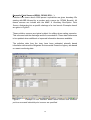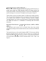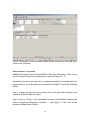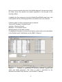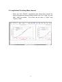
Download Annex 6 Practical Guideline for MIKE 11 Water Quality Model

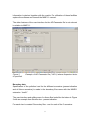
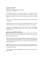
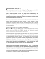
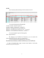
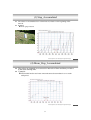
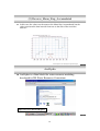
Annex 6
Practical Guideline
for
MIKE 11 Water Quality Model
JICA Study Team
1
2
MIKE 11 Files used for Water quality Modelling
The MIKE 11 water quality modelling utilizes the files created during the MIKE
hydrodynamic model set-up. Few adjustments have been made for the most
upstream part of the rivers to ensure sound and stable water quality simulation.
The files used for the water quality modelling is therefore stores in a special
directories named:
C:¥MIK11WQ_Bulagria
C:¥MIK11_Bulgaria_WQ-template
Simulation files
The primarily simulation files used for the model set-up, calibration and scenario
simulation is specified in the MIKE 11 sim-files (*.sim11)
There has been prepared sim- files for following the Struma River, Mesta-Dospat
River, Tundzha River, Maritza River and Arda-Biala River representing the
scenarios:
•
•
Prensent
Near Future
•
•
•
Near Future with 10 % loss
High Priority Future
High and Medium Priority Future
The difference between the sim-files for different scenarios is the selection
Boundary file (se below). For description of these scenarios please see the
MAIN REPORT and SUPPORTING REPORT of this project.
The appearance of that part of the user-interface of the sim-file, where the
differences simulation files is selected, is shown in Figure 1.
The Network file, The Cross-section files and the HD-parameter file is not
described in any details here in this section. Please refer to the guideline for the
Hydrodynamic Model and the MIKE 11 Manual.
3
Figure 1
Example of simulation file (*.sim11) where specific file is
selected the model simulation.
AD Parameters
When using the EcoLab water quality modelling facilities of MIKE 11 the only
parameter that is to be specified in the AD parameter file is the Dispersion factor.
Figure 2 shows an example of the user-interface where this value is specified.
For the rivers in general are used a dispersion factor of 25. For some of the
rivers local higher values have been used at a few most upstream calculation
points in the rivers and at some structures within the rivers, e.g. weirs.
Specification of Components, initial condition and decay is not utilised. The initial
(e.g. the start) concentrations as well as the components are specified in the
EcoLab modelling file.
The <Additional output> facilities can be utilised by the model user it more
4
information is desired together with the results. For utilisation of these facilities
explore the software and consult the MIKE 11 manual.
The other features of the user interface for the AD Parameter file is not relevant
in relation to MIKE 11.
Figure 2
is specified.
Example of AD Parameter file (*.AD11) where dispersion factor
Boundary data
Specification of the pollution load for the different scenarios (present situation
and all future scenarios) is made in the boundary files name with the MIKE11
extension “.bnd11”
The user interface and editing menu for these files looks like the below in Figure
3 with an example from Struma river - present situation.
For each river is created 5 boundary files - one for each of the 5 scenarios.
5
Figure 3
Example of user interface where open model boundaries as well
as lateral inflow boundaries can be specified.
In this menu is specified where (river branch name and chainage) the inflow to
the model/river occur.
For each inflow item the discharge and the concentration of pollutants is
specified in the two windows in the second half of this menu.
For the pollutants in the lower part of the menu is the concentration for different
component number specifies. These component numbers refer to the EcoLab
template that is used. For the model set-up for these Bulgarian rivers the
component number corresponds to the following substances:
Component 1 : Oxygen
Component 2: Temperature
Component 3: Ammonium-N
6
Component 4: Nitrate-N
Component 5: BOD
Component 6: Dissolved (ortho) phosphate-P
Component 7: Particulate-P
For additional description of the EcoLab template, the component and the
processes transforming these components, please refer to the MIKE 11 manual
and to the compendium with power point presentations given during the training
course.
To the most left in the upper part of the boundary file editor you find Boundary ID
– information.
This information has in the model set-up be organised and defined in a way that
should facilitate the overview and future editing for creation of new scenarios.
Each group of boundaries have in the Boundary ID been given different
recognisable code numbers together with a more common under stood
identification name.
Model boundaries (M0001, M002, M00…)
The first boundary items concerns the inflow at the model boundary. All this type
of boundaries starts with an M followed by a number and name, (ex.:
M004_UpstreamEnd_ST_M).
These are primarily important for the upstream boundary, but values have also to
be specified at down stream boundaries. However the inflows at the boundaries
are in these set-ups general low and will not influence the simulated condition
further down stream.
I addition there exist some internal boundaries defined in hydrodynamic model
(MIKE 11 HD). These will not be comment further here. Refer to the HD set-up
for additional information.
For most future scenarios no changes is to be made in these boundary items
starting with M.
7
Abstractions (A001, A002, A00…)
The next group concerns the water abstraction. These are named with A
followed by a number and a name, (ex.: A001_Abst_ST_ARK).
Most of these are outflows from the river as the nature of abstractions. The
discharges at such boundaries are negative. However some are positive or
periodically positive which mean inflow. Therefore concentration for these has as
well been specified in the boundary files.
For none of the scenarios that have been defined and simulated within the
project, these boundaries have been changed. It could however in future
scenarios be relevant to change both the abstraction amount and in case the
abstraction is positive (e.g. inflow to the river), it could also be relevant to change
the concentrations.
Distributed Domestic Sources (DD001, DD002, DD0…)
The group of boundary item with Boundary ID named DD (followed by a number
and a name (ex. DD006_Dis_ST_ELE) describe the distributed domestic
pollution sources in the catchment (NAM-catchments).
Domestic population living outside the main villages and towns (e.g. individual
houses and villages with less than 2000 persons) are included in the model as
so called distributed domestic sources. The contribution from these is equally
spread along the main river sections. These are general inserted with the MIKE
11 Boundary Description: distributed source, (see Figur 4). For this type of
MIKE 11 boundaries there are required an upstream and downstream chainage
between which the inflow is equally distributed. These chainages are typical
up- and downstream chainage for inflow from each NAM-catchment.
However some of the boundaries with the Boundary ID “DD0… “ are give in the
model as MIKE11 Point sources. This is the case when the MAM catchment isn’t
distributed along a river stretch, but is inflowing in one point of the model. This
will be the case for rivers which is not included as MIKE 11 river branches in the
set-up but only represented by a NAM-catchment. Example is shown in Figure 2
for the items 55, 56 and 57 from the Struma River set-up.
8
Figure 4
Example of user interface where lateral inflows from distributed
domestic sources are specified.
The discharges used from these sources have been calculated based on
statistical data and a unit amount of sewage water produced per person.
The concentrations have been estimated using unit pollution load per person for
the individual components (variables) together with an assumed average loss
percentage in the catchment its way form the pollution source to the river.
These pollution sources are one of the typical issues for editing when crating
scenarios. This concerns both the discharge and the concentration. These data
can furthermore to be updated when additional or improved information
becomes available.
9
Domestic Point Sources (DP001, DP002, DP0… )
Pollution from towns above 2000 person equivalents are given boundary IDs
starting with DP followed by a number and a name (ex. DP009_Breznik). All
theses sources are include with the MIKE 11 Boundary Description: Point
Source, discharging into a specific chainage of a river branch. Examples hereof
are given in Figure 5.
These pollution sources are typical subject for editing when crating scenarios.
This concerns both the discharge and the concentration. These data furthermore
to be updated when additional or improved information becomes available.
The pollution data from the town have been estimated primarily based
information delivered the Bulgarian Environmental Executive Agency are based
on resent monitoring data.
Figure 5
Example of user interface where lateral inflows from domestic
point sources and industrial point sources are specified.
10
Industrial Point Sources (IP001, IP002, IP0… )
Pollution from industries are given boundary IDs starting with IP followed by a
number and a name (ex. IP082_Dimankov SPLTD). All theses sources are
include with the MIKE 11 Boundary Description: Point Source, discharging into a
specific chainage of a river branch. Examples hereof are given in Figure 5.
These pollution sources are typical subject for editing when crating scenarios.
This concerns both the discharge and the concentration. These data furthermore
to be updated when additional or improved information becomes available.
The data inserted in the model are primarily based on data delivered by EABD
and WABD and based on a combination of monitoring data and licence
information.
Agricultural Point Sources = Livestock Point Sources (XLSP01, XLSP02,
XLSP0…)
The agricultural point sources such as livestock farms have been include
individually according to the information that have been received from EADB and
WADB.
The livestock farms are in the model included as MIKE 11 Point sources with the
Boundary ID starting with the start letter of the river names (e.g. for Struma: S),
followed by LSP (livestock point source), a number, a name and characterisation
of the animal type, (for example: SLSP05 "Kembarou MM 5" JSCo – Pigs) – see
Figure 6.
11
Figure 6 Example of user interface where lateral inflows from livestock point
sources are specified.
Point sources - in general
Additional boundary items, with the MIKE 11 Boundary Description: Point source,
can be inserted manual in the editing menu shown in Figure 4 - 6.
Alternatively the point sources can be created and edited for example an Excel
spread sheet or a text file editor and copied into the MIKE 11 using the following
facility.
Step 1: Create one point source boundary item of the type that is wanted to be
copied in. Mark this with the curser.
Step 2: click on <Tools> in the command line menu of the MIKE11 window and
select <Copy/paste Boundary Condition> – see Figure 7. Click and a new
window will appear like Figure 8.
12
Step 3: Copy from for example an excel sheet with the same format as outlined
in the “copy/paste Boundary Condition - window” and past into the window
shown in Figure 8. When you hereafter close the Figure 8 window, the new
boundary items will appear in the boundary editor/file.
Step 4: Check the unit. If the unit is not correct or as expected, then delete the
inserted boundary items. Check and modify to necessary extent the values in the
Excel file and repeat the procedure.
Figure 7
Activation of facility for Copy/paste Boundary Condition
13
Figure 8
Copy/paste Boundary Condition – window.
Non-point sources
Non-point sources are in general flowing into the river branches together with the
inflow from the Rainfall-Runoff / NAM catchments.
The water inflow has already been specified in the NAM-MIKE 11 HD interface.
These inflow chainages can be seen from opening the network file (*.nwk11),
click <View> and <Tabular View> from the MIKE 11 command line – (Please for
additional information refer to the HD-model specification and the MIKE 11
manual).
Because the amount of water already is given form the NAM-MIKE11HD
interface no water is to be specified for the non-point pollution – specification has
only to be made for the pollutants (the AD components). This is ensured by
activating (checking in) the AD-RR option in the second window of the menu. By
doing so, the appearance of the editor will look some what like Figure 8.
14
Here you have to specify the name of the NAM-catchment, the area from which
the inflow occurs the specific river stretch (specified in the top part of the
boundary editor).
In addition the flow component from the Rainfall-Runoff/NAM model has to be
used together with the following specified concentration has to be selected.
Following option for flow components can be selected:
Total runoff, Overland = Surface Runoff,
Interflow = Rootzone Runoff,
Baseflow = Groundwater Runoff,
Rainfall (directly on the water surface).
For additional information on these runoff options, please refer to the description
of the Rainfall runoff / NAM Model and the MIKE 11 Manual.
Figure 9
Example of specification of Non-point pollution together with
inflow from NAN catchment. (The inflow of water is described by the
Rainfall-Runoff MIKE11DH interface- see the MIKE 11 Manual)
15
In the model set-up for the Bulgarian rivers non-point sources with two groups of
Boundary ID have been used as shown in Figure 9 and 8:
[Load: Nonpoint, Baseflow]
[Load: Nonpoint, Overland]
[Load: Nonpoint, Interflow]
[Load: Nonpoint, Overland]-fertil
[Load: Nonpoint, Interflow]-fertil
[Load: Nonpoint, Baseflow]-fertil
The boundary items with the Boundary ID
[Load: Nonpoint, Baseflow]
[Load: Nonpoint, Overland]
includes the pollution from non-point contribution from livestock. This has been
based on statistical information on livestock density, unit load from the different
types of animal and a runoff coefficient of 5 %.
16
Figure 10
Example of specification of Non-point pollution fro the use of
fertiliser together with inflow from NAN catchment. (The inflow of water is
described by the Rainfall-Runoff MIKE11DH interface- see the MIKE 11 Manual).
The boundary items with the Boundary ID
[Load: Nonpoint, Interflow]
Includes the inflow of different potential pollution components with the
groundwater.
The boundary items with the Boundary ID
[Load: Nonpoint, Overland]-fertil
[Load: Nonpoint, Interflow]-fertil
includes the potential pollution components from the use of fertilisers. The use of
fertiliser is from statistical data. The amounts and concentrations discharged into
the rivers have been estimated using a runoff coefficient of 10 %.
17
The boundary items with the Boundary ID
[Load: Nonpoint, Baseflow]-fertil
Include oxygen concentration and temperature assumed in the groundwater.
The name “-fertile” is therefore misleading as it has noting to do with fertilisers.
The values have only been inserted here under this name due to practical and
pragmatic reasons.
Figure 11
Example of specification of temperature and oxygen content of
groundwater inflow from NAN catchment. (The inflow of water is described by
the Rainfall-Runoff MIKE11DH interface- see the MIKE 11 Manual).
18
Creation of Non Point Boundary conditions (items) using LOAD
CALCULATOR
The non point boundary conditions can be edited directly in the *.bdn11 file
described above. However MIKE BASIN (which is delivered to the EABD and
WABD together with the MIKE 11 software) includes a tool for assisting in
quantification of the non-point load to different river stretches in a MIKE 11
set-up. This facility has been used for distribution of the non-point livestock
pollution and the fertiliser runoff along the MIKE 11 branches. The result hereof
is illustrated above. It is not necessary to use this facility for changing the load
and create input to new scenarios. This can be done directly in the MIKE 11
Boundary Editor described above.
It is not the intention here to give a detailed introduction to the LOAD
CALCULATOR, which is a DHI produces ArcGIS-extension. Please refer to the
available manual etc. that follows with the software.
The following description only outlines how the software has been used for the
model set-up in these specific cases.
19
Figure 12 MIKE BASIN - LOAD CALCULATOR. Example: Tundzha.
20
The NAM-catchment is transfer into MIKE Basin catchment type (through a
standard ArcGIS procedure).
The NAM catchment layer is opened in ArcGIS /MIKE BASIN. An ArcGIS layer
with information of the Livestock density or Fertiliser use in different areas is
opened. These layers do not need to have the same resolution. An example
where the livestock layer and the NAM catchment for Tundzha have been
opened is shown in Figure 12.
By mouse click on MIKEBASIN will open the MIKEBASIN menu (Figure
12,lower), from where the Load Calculator can be activated (Figure 13).
Figure 13
set-up.
DHI Load Calculation menu. Example: Tundzha Livestock
21
The DHI LOAD CALCULATOR is now open for editing (Figure 13). In this
example the livestock layer (BGMun_LS) is specified. Fields and values in the
attribute table have to be selected for the different species of animals. For more
details, please consult the set-up of the LOAD CALCULATOR for the individual
rivers and the manual and information that follow with the software. (Information
can also be achieved from DHI homepage: www.dhigroup.com).
Mouse click on the <View table> (ĺ in Figure 13) gives an overview of unit
pollution load data used for the estimation of the non-point load (Figure 14).
Click on <Import Result> (Figure 13) and browse for the relevant NAM-results.
Click on <Set component> (Figure 13) and set the component correct according
to the used ECOLab model.
Ensure that <MIKE11> in checked in the lower right corner of the DHI Load
Calculator window.
Browse for the correct MIKE 11 sim-file. Select the MIKE 11 sim-file with the
boundary file where the new boundary items have to be added.
Press <Calculate> and the boundary item is added to the selected MIKE 11
boundary file.
It is highly recommended carefully to consult the LOAD CALCULATOR manual
and explore the different opportunities before creation of scenarios by using the
described facility. You will find a lot of possibilities, which among other includes
option for time varying outflow for the non-point source over the year, changes in
runoff coefficients, option for specification of decay within the catchments and
concentration in groundwater inflow etc.
In addition to the inserting of the boundary items into the MIKE11 boundary file
the LOAD CALCULATOR also give the calculated yearly load from each NAM
catchment. Example is shown in Figure 15. The results can be exported to
dbf-files and Excel-files.
22
Figure 14
catchments.
Example of the unit load used for livestock in the Tundzha
Figure 15
Example on simulated yearly load from domestic livestock in
Tundzha River Basin.
23
The LOAD CALCULATOR set-up for the Bulgarian catchments can be launched
from the directories named “MIKE_rivername_LoadCal” by loading the
“MB_rivername_load.mxd” files into MIKE BASIN / ArcGIS. Using the
geodatabase
“MB_rivername_load.mdb” will activate the set-up for calculation
of the non-point load from the livestock. Using the geodatabase
“MB_rivername_load-fertile.mdb” will activate the set-up for calculation of the
non-point load from the use of fertiliser.
ECOLab parameter file (water quality model)
The water quality model used is specified through the *.ecolab11 files. Theses
are as the other modelling files specified in the *sim11 file (Figure 1).
From the MIKE 11 software different predefined types of water quality models
(model templates) can be selected as described in the MIKE 11 Manual.
For the Bulgarian Rivers the templates have been slightly modified for the
description of condition in the specific rivers. Please consult the delivered model
set-ups for specification of the template used for the individual rivers.
The
modified
ECOLab
templates
“C:¥MIK11_Bulgaria_WQ-template”
are
found
the
directory:
Figure 17 illustrates the variables that are described by the models. The
parameters (variables) shown in Figure 17 are stores in MIKE 11 result files
named *.res11, where as the parameters (variables) shown in Figure 18 are
stored in result files named *Add.res11. The Total BOD is calculated as the BOD
from pollution sources plus the BOD from background contribution (∼1mg/l).
The result files are viewed using the MIKE 11 software MIKE VIEW. For
information of using this software please consult the MIKE 11 Manual.
24
Figure 16
User interface of the ECOLab Parameter file
Figure 17
Parameters (State variables) that are simulated by the models.
In the column values the start (initial) values are set. They are stored in result file
named *.res11
Figure 18
Additional Parameters (derived output) that are simulated by the
models. They are stored in result file named *Add.res11 when they are checked
as shown here.
25
26
Annex 7
Manual
for
Simple Model_ver_Permit
(A Simple Water Quantity Assessment Tool)
JICA Study Team
1
2
1. General
Simple Model_ver_Permit is prepared to examine the effect of permitted
water amount on water quantity condition in rivers. By imputing permission
data, the model can summarize the total permitted water quantity at observation
points.
There are two versions for Simple Model_ver_Permit.
•
•
Version 1: Simple Model_ver_Permit
Version 2: Simple Model_ver_Permit2
In Version1, the model gives the following two results, together with
existing flow condition during 2001-2005.
•
Local (Permitted water abstraction from local water object) + Existing
water abstraction from significant reservoir
•
Local (Permitted water abstraction from local water object) + Permitted
water abstraction from significant reservoir
In Version2, the following result can be compared with expected flow
conditions for several probabilistic precipitation conditions.
•
Local (Permitted water abstraction from local water object) + Permitted
water abstraction from significant reservoir
The quasi-natural, potential with significant reservoir, disturbed flows for
the existing condition during 2001-2005 and the expected probabilistic condition
are estimated by other versions, Simple Model_ver_Exsiting and Simple
Model_ver_Potential, which have been also prepared by JICA Study Team.
The ver_Permit just utilizes those results. The comparison between the
permitted water quantity and the quasi-natural, potential with significant reservoir,
disturbed flows may give an idea on strategy for river management. However,
even if there are no data for quasi-natural, potential with significant reservoir,
disturbed flows, calculation of total amount of permitted water at observation
points is possible and it may give also valuable information for river managers.
3
The main features are as follows:
•
•
•
Entering permission data for HPP, IRR, DWS, IWS
Selection of reference points for management
Summary table for annual average and average during summer time (Jul.
to Sep.) for year 2001 -2005 for each catchment/segment and reference
point
•
•
•
•
Longitudinal plot of the summarized results along main channel
Time series plot for each reference point and/or catchment/segment
Globally and locally changeable coefficient for permitted water amount
Preparation of an input file related to local water abstraction for each
NAM catchment for MIKE11 water quantity model prepared by JICA
Study Team
This manual is written for “Simple Model_ver_Permit”. Operation of “Simple
Model_ver_Permit2” is same as “Simple Model_ver_Permit”.
Only
presentation of results is different.
4
2. Definition of terms
In this model, the following definition is used.
„ Quasi-Natural Flow
‡ Flow without disturbance such as abstraction, discharge, transfer
‡ Likely natural, however, not exactly natural.
‡ In the model, regime change of local reservoir is not taken into
account.
„ Potential Flow with Significant Reservoir
‡ Flow with influence of significant reservoir, including transfer from
and to a reservoir, but no abstraction of water
‡ Potentially usable water amount after regime change by significant
reservoir
„ Disturbed Flow
‡ Existing condition
‡ Potential Flow – Total abstracted water + Total discharged water
Abbreviation
HPP:
IRR:
S_Res:
NAM Catchment:
Hydro Power Plant
Irrigation
(Note: Irrigation water use includes only water for
Irrigation area managed by Irrigation Systems)
Drinking Water Supply
Industrial Water Supply
(Note: Industrial Water supply includes agricultural and
fish breeding water use)
Significant Reservoir
Catchment for NAM (Rainfall-Runoff) model
NF:
PF:
DF:
Quasi-Natural Flow
Potential Flow with Significant Reservoir
Disturbed Flow
DWS:
IWS:
5
3. Remarks for treating Excel sheet in the model
The model just utilizes excel spread sheets and macros. Some sheets
are hidden, because the hidden sheets are usually not necessary to be edited by
users. If you want to see the hidden sheets, please do the followings.
Format -> Sheet -> Unhide
Then, select the sheets you want to open.
In each spread sheet, you may see cells with different colors.
meaning of the colors is as follows.
White:
User can edit
Light blue:
Yellow:
Value in cell is automatically calculated.
Value in cell is calculated by macros.
DO NOT edit the cells with light blue and yellow.
the model will give wrong results.
6
The
If you change it,
4. Model Outline
1) Struma River
File Name:
Struma_WaterBalance_Permit.xls
Struma_WaterBalance_Permit2.xls
Number of catchment = 104
Number of NAM catchment = 25
2) Mesta & Dospat River
File Name:
Mesta&Dospat_WaterBalance_Permit.xls
Mesta&Dospat_WaterBalance_Permit2.xls
Number of catchment = 75
Number of NAM catchment = 14
3) Arda & Biala River
File Name:
Arda&Biala_WaterBalance_Permit.xls
Arda&Biala_WaterBalance_Permit2.xls
Number of catchment = 69
Number of NAM catchment = 12
4) Tundzha River
File Name:
Tundzha_WaterBalance_Permit.xls
Tundzha_WaterBalance_Permit2.xls
Number of catchment = 84
Number of NAM catchment = 19
5) Maritsa River
File Name:
Maritsa_WaterBalance_Permit.xls
Maritsa_WaterBalance_Permit2.xls
Number of catchment = 251
Number of NAM catchment = 34
7
5. Input of permission data
1)
2)
3)
4)
You can see the following five tabs for input of permission data.
Permit_HPP
Permit_IRR
Permit_DWS
Permit_IWS
5) Transfer_NoRecord
(1) HPP
Input necessary data according to the items shown in Line10.
You must al least input the following data.
Location of Intake : Intake-ID (column H)
Location of Intake : Catchment-ID (column N)
Location of Discharge : Catchment-ID (column T)
WaterUse : Permitted Amount (m3/s) (column X)
WaterUse : Permitted Annual Volume (106 m3) (column Y)
WaterUse : Local Coefficient for Permission
8
(column AC)
By changing Local Coefficient for Permission, you can examine the
effect of permitted amount for each one of permissions.
The calculated water used will be:
(Permitted amount) x (Global Coefficient) x (Local Coefficient)
(2) IRR
Input necessary data according to the items shown in Line10.
You must al least input the following data.
User : Branch (column H)
Location of Intake : Intake-ID (column J)
Location of Intake : Catchment-ID (column P)
WaterUse : Permitted Amount (m3/s) (column R)
WaterUse : Permitted Annual Volume (106 m3) (column S)
WaterUse : Local Coefficient for Permission (column U)
By changing Local Coefficient for Permission, you can examine the
effect of permitted amount for each one of permissions.
The total calculated water abstraction per year will be:
(Permitted Annual Volume) x (Global Coefficient) x (Local Coefficient)
In case of irrigation, water abstraction pattern within a year will be given
based on actually used water for each one of Irrigation Branches in 2001-2005.
The data for actually used water was obtained from Irrigation Systems.
Spatial pattern of water use within an Irrigation branch is assumed to be
proportional to the permitted amount for each one of permissions.
9
(3) DWS
Input necessary data according to the item shown in Line10.
You must al least input the following data.
Location of Intake : Intake-ID (column I)
Location of Intake : Catchment-ID (column O)
WaterUse : Permitted Amount (m3/s) (column P)
WaterUse : Permitted Annual Volume (106 m3) (column Q)
WaterUse : Local Coefficient for Permission
(column S)
By changing Local Coefficient for Permission, you can examine the
effect of permitted amount for each one of permissions.
The total calculated water abstraction per year will be:
(Permitted Annual Volume) x (Global Coefficient) x (Local Coefficient)
In case of drinking water supply, constant value based on total water
abstraction per year will be given.
10
(4) IWS
Input necessary data according to the item shown in Line10.
You must al least input the following data.
Location of Intake : Intake-ID (column J)
Location of Intake : Catchment-ID (column P)
WaterUse : Permitted Amount (m3/s) (column Q)
WaterUse : Permitted Annual Volume (106 m3) (column R)
WaterUse : Local Coefficient for Permission (column T)
It is recommended to input the following data.
User : Type (column H)
By changing Local Coefficient for Permission, you can examine the
effect of permitted amount for each one of permissions.
The total calculated water abstraction per year will be:
(Permitted Annual Volume) x (Global Coefficient) x (Local Coefficient)
In case of industrial water supply, constant value based on total water
abstraction per year will be given.
11
(5) Transfer_NoRecord
If there is a water transfer between catchments by local HPP, but no
record exists, you can specify the transferred water amount here.
Input necessary data according to the item shown in Line9.
You have to at least specify the following data.
From : Catchment-ID (column D)
To : Catchment-ID (column F)
Transfet Mode (column G)
If TransferMode =1
MaximumLimit (column H)
If Transfer Mode =2
Percent (column I)
This water transfer is not taken into account for water abstraction. However, it
is taken into account when MIKE11 input file is prepared.
12
6. Setting reference points for management
Default reference points have been set by JICA Study Team. However,
in the model, you can set reference points as you like in ”
Summary_RefPoints” tab.
The value calculated for each one of catchments represents the value at
the downstream end of river segment in the catchment.
When you select a reference point around river confluence, you have
two choices.
One is before confluence.
Another is after the
confluence.
If you select the point before the confluence, you have to specify
Catchment ID for upstream segment and “D” for “Downstream or
Upstream”. Similarly, you have to select Catchment ID for downstream
segment and “U” when the point after the confluence is selected.
13
Example:
Before confluence: Catchment ID =1 and “D”
After confluence: Catchment ID =3 and “U”
D
1
2
U
3
You can choose “No.” as you like. However, this “No.” will be used
when you plot time series data.
“NAM catchment” is used for reference for default setting. If you do not
consider “NAM cacthment”, this can be left as blank.
14
7. Calculation
In “Control” tab, you can calculate to summarize the permission data.
In column “K”, maximum number of permission and/or reference points
can be set. The maximum number must be greater than the number
which has been inputted in each input page.
In column “ J”, Global coefficient for permission can be specified.
When you click the button “PM001” to “PM005”, the permission values
are calculated and summarized. You must calculate once after
permission data are updated. You can refer the “Last updated
Date&Time”.
After calculation completed, Summary table in “Summary” and
“Summary_2” are updated. Summary table shows annual average and
average during summer time (Jul. to Sep.) for year 2001 -2005.
There are two results groups: Result_1 and Result_2
Result_1 is for:
Local (Permitted water abstraction from local water object) + Existing
water abstraction from significant reservoir.
Result_2 is for:
Local (Permitted water abstraction from local water object) + Permitted
water abstraction from significant reservoir.
15
When you click “PM101”, summary results for reference points are
calculated.
After complete the calculation, please see
“Summary_RefPoints” and “Summary_RefPoints_2”.
16
8. Longitudinal Plot along Main channel
When you click “PM102”, longitudinal plots along main channel for
annual average and average during summer time (Jul. to Sep.) for year
2001 -2005 are plotted. The results can be seen in “Figure” and
“Figure_2” tabs.
17
9. Time Series Plot
Time series can be plotted in “TimeSeries_Plot” tab.
You have to firstly specify the location for time series plot.
You have two choices. One is to select a point from the reference
points(1:RefPoint). Another is to specify Catchment ID (2:segment).
Please select “1” or “2” in the cell ”A2”.
Then, please specify “No. of RefPoints” or “Catchment ID”.
After specifying the location, click button “Re-plot TimeSeries”.
You will see new plots.
18
10. Preparation of MIKE11 Input file
In “Control” tab, click button “PM201”. Then, MIKE11 input file will be
updated in “Sum_AbstW_NAMcatchment_MIKE11” tab.
You can copy the updated value and paste it to “xxxx_AbstW.dfs0”.
Using the updated “xxxx_AbstW.dfs0” with MIKE11 model, you can
investigate the effect of several water use condition on water quantity
along river in detail.
Please remind that MIKE11 model automatically stops abstraction when
19
amount of water is not enough. In this case, you will see “warning”.
However, it is OK for water quantity simulation, if you can recognize that
the actually abstracted water amount is smaller than that is given as
boundary condition.
It is highly possible that the above-mentioned case occurs if you assume
total permitted water amount is abstracted.
20
Annex 8
Manual
for
Simple Model_ver_Demand
(A Simple Water Quantity Assessment Tool)
JICA Study Team
1
2
1. General
Simple Model_ver_Demand is prepared to examine the balance
between water demand and water resources potential. By imputing parameters
related to estimation of water demand, the model can summarize the total water
demand at observation points.
The quasi-natural flow, potential flow with significant reservoir for the
average year (2004) and the expected probabilistic flow are estimated by other
versions, Simple Model_ver_Exsiting and Simple Model_ver_Potential, which
have been also prepared by JICA Study Team. The ver_Demand just utilizes
those results.
The comparison between the water demand and the
quasi-natural, potential with significant reservoir may give an idea on strategy for
river management.
The main features are as follows:
•
•
•
Entering parameters for estimation of water demand for IRR, DWS, IWS
Selection of reference points for management
Summary table for annual average and average during summer time (Jul.
to Sep.) for each catchment/segment and reference point
•
•
•
Longitudinal plot of the summarized results along main channel
Time series plot for each reference point and/or catchment/segment
Preparation of an input file related to local water abstraction for each
NAM catchment for MIKE11 water quantity model prepared by JICA
Study Team
3
2. Definition of terms
In this model, the following definition is used.
„ Quasi-Natural Flow
‡ Flow without disturbance such as abstraction, discharge, transfer
‡ Likely natural, however, not exactly natural.
‡ In the model, regime change of local reservoir is not taken into
account.
„ Potential Flow with Significant Reservoir
‡ Flow with influence of significant reservoir, including transfer from
and to a reservoir, but no abstraction of water
‡ Potentially usable water amount after regime change by significant
reservoir
„ Disturbed Flow
‡ Existing condition
‡ Potential Flow – Total abstracted water + Total discharged water
Abbreviation
HPP:
IRR:
S_Res:
NAM Catchment:
Hydro Power Plant
Irrigation
(Note: Irrigation water use includes only water for
Irrigation area managed by Irrigation Systems)
Drinking Water Supply
Industrial Water Supply
(Note: Industrial Water supply includes agricultural and
fish breeding water use)
Significant Reservoir
Catchment for NAM (Rainfall-Runoff) model
NF:
PF:
DF:
Quasi-Natural Flow
Potential Flow with Significant Reservoir
Disturbed Flow
DWS:
IWS:
4
3. Remarks for treating Excel sheet in the model
The model just utilizes excel spread sheets and macros. Some sheets
are hidden, because the hidden sheets are usually not necessary to be edited by
users. If you want to see the hidden sheets, please do the followings.
Format -> Sheet -> Unhide
Then, select the sheets you want to open.
In each spread sheet, you may see cells with different colors.
meaning of the colors is as follows.
White:
User can edit
Light blue:
Yellow:
Value in cell is automatically calculated.
Value in cell is calculated by macros.
DO NOT edit the cells with light blue and yellow.
the model will give wrong results.
5
The
If you change it,
4. Model Outline
1) Struma River
File Name:
Struma_WaterBalance_Demand2.xls
Number of catchment = 104
Number of NAM catchment = 25
2) Mesta & Dospat River
File Name:
Mesta&Dospat_WaterBalance_Demand2.xls
Number of catchment = 75
Number of NAM catchment = 14
3) Arda & Biala River
File Name:
Arda&Biala_WaterBalance_Demand2.xls
Number of catchment = 69
Number of NAM catchment = 12
4) Tundzha River
File Name:
Tundzha_WaterBalance_Demand2.xls
Number of catchment = 84
Number of NAM catchment = 19
5) Maritsa River
File Name:
Maritsa_WaterBalance_Demand2.xls
Number of catchment = 251
Number of NAM catchment = 34
6
5. Input of parameters for estimating water demand
You can see the following two tabs for input of parameters related to
water demand.
1) Demand_IRR
2) Demand_DWS
(1) IRR
Irrigation water demand is calculated based on the followings for each
irrigation system.
1)
2)
3)
4)
Unit water demand (m3/year/dca)
Potential irrigation area (dca)
Percentage of actual irrigation area against potential irrigation area (%)
Loss rate (%)
Among those, 2) Potential irrigation area fro each irrigation system has
already set together with its location of main water sources. You do not
need to change these.
You have to input 1), 3) and 4).
7
(2) DWS
Drinking water demand is calculated based on the followings for each
settlement.
1) Unit water use (litter/day/person)
2) Percentage of Surface water use (%)
3) Loss rate (%)
You have to input all of 1), 2) and 3).
8
6. Setting reference points for management
Default reference points have been set by JICA Study Team. However,
in the model, you can set reference points as you like in ”
Summary_RefPoints” tab.
The value calculated for each one of catchments represents the value at
the downstream end of river segment in the catchment.
When you select a reference point around river confluence, you have
two choices.
One is before confluence.
Another is after the
confluence.
If you select the point before the confluence, you have to specify
Catchment ID for upstream segment and “D” for “Downstream or
Upstream”. Similarly, you have to select Catchment ID for downstream
segment and “U” when the point after the confluence is selected.
9
Example:
Before confluence: Catchment ID =1 and “D”
After confluence: Catchment ID =3 and “U”
D
1
2
U
3
You can choose “No.” as you like. However, this “No.” will be used
when you plot time series data.
“NAM catchment” is used for reference for default setting. If you do not
consider “NAM cacthment”, this can be left as blank.
10
7. Calculation
In “Control” tab, you can calculate to summarize the water demand by
catchment.
In cell “J4”, maximum number of reference points can be set. The
maximum number must be greater than the number which has been set.
In line”7”, you can set the following two coefficients for estimating
industrial water demand.
1. Coefficient for Economic Growth (CE)
2. Coefficient for Recycling Water Use (CR)
Industrial Water demand is calculated as follows.
(Industrial water demand) = (existing industrial water use) x CE x CR
When you click the button “PM001” to “PM002”, the water demand are
calculated and summarized. You must calculate once after parameters
for water demand are updated. You can refer the “Last updated
Date&Time”.
After calculation completed, Summary table in “Summary” are updated.
Summary table shows annual average and average during summer time
(Jul. to Sep.).
11
When you click “PM101”, summary results for reference points are
calculated.
After complete the calculation, please see
“Summary_RefPoints” .
12
8. Longitudinal Plot along Main channel
When you click “PM102”, longitudinal plots along main channel for
annual average and average during summer time (Jul. to Sep.) are
plotted. The results can be seen in “Figure” tabs.
13
9. Time Series Plot
Time series can be plotted in “TimeSeries_Plot” tab.
You have to firstly specify the location for time series plot.
You have two choices. One is to select a point from the reference
points(1:RefPoint). Another is to specify Catchment ID (2:segment).
Please select “1” or “2” in the cell ”A2”.
Then, please specify “No. of RefPoints” or “Catchment ID”.
After specifying the location, click button “Re-plot TimeSeries”.
You will see new plots.
14
10. Preparation of MIKE11 Input file
In “Control” tab, click button “PM201”. Then, MIKE11 input file will be
updated in “Sum_AbstW_NAMcatchment_MIKE11” tab.
You can copy the updated value and paste it to “xxxx_AbstW.dfs0”.
Using the updated “xxxx_AbstW.dfs0” with MIKE11 model, you can
investigate the effect of several water use condition on water quantity
along river in detail.
15
Please remind that MIKE11 model automatically stops abstraction when
amount of water is not enough. In this case, you will see “warning”.
However, it is OK for water quantity simulation, if you can recognize that
the actually abstracted water amount is smaller than that is given as
boundary condition.
It is highly possible that the above-mentioned case occurs if you assume
total permitted water amount is abstracted.
16
Annex 9
Supplimentary Material
JICA Study Team
1
2
Introduction – Time Series Data
3
Level 6 Water Management Plan Data
Feed back
Feed back
Level 5 Spatial Distribution Analysis Data
Level 4 Basic Analysis Data at Point
Water Quantity and
Quality Model
Data Level
Time Series Data
Level 3 Monitoring Data
Level 2 Water Bodies Data
Level 1 Core Data
4
3
Structure of Modeling Environment
MIKE11 & MIKE BASIN
Ms-Excel
Boundary
Condition
MIKE11
(MIKE Zero platform)
- Preparation of input
file for simulation
Simple Model
(Spread sheet)
MIKE BASIN
Temporal Analyst &
Pollution load calculator
Parameters
(Quasi-Natural
Run-off etc.)
Connection of
output file to GIS
environment
(ArcGIS extension:
part of MIKE11 GIS after ver2007)
Extract DB or
Connection to DB
Final
Assembling
- Extract base layer
- Connection to DB
GIS-DB
- Water Body
- Natural & Socio-economical information
- Monitoring Data for Water Quantity and Quality
- Permission Data
- Operation record for reservoir and irrigation
5
Time Series Data used in the Model
„
Meteo-Hydrological data
‡ Daily Precipitation
‡ Monthly Potential Evapo-Transpiration
‡ Daily Air Temperature
‡ Daily Water Quantity at key HMS
„
Water Abstraction/Discharge data
‡ Reservoir Operation Data
‡ Water Abstraction Data
¾ Irrigation Use
¾ Domestic & Industrial Water Use
‡ Water Discharge (Waste Water) Data
„
Water Quality Monitoring data
……etc.
6
4
Example of Source data:
Daily Water Quantity from NIMH
Table is good. But, difficult to utilize for analysis…
ȻəɅȺ ɊȿɄȺ - ɋ. ȻɈɋɌɂɇȺ
N 61050
2000ȽɈȾ.
ȼɈȾɇɂ ɄɈɅɂɑȿɋɌȼȺ, ɦ3/s
I
II
III
IV
V
VI
VII
VIII
IX
.041
X
XI
.021
XII
1
1.030>
.192
.552
2.075
1.140
.338
.122>
.029
2
.828
.400
.552
2.075
1.255
.235
.095
.029
.041
.021
.021
.021
.029
.029
3
.732
.640
.732
1.926
1.780
.235
.073
.029
.029
.021
.021
.029
4
.640
.732
.640
1.637
1.140
.235
.056
.021
.029
.021
.021
.029
5
.640
.552
.732
1.926
.927
.235
.056
.015<
.029
.021
.021
.029
6
.552
.552
.640
1.780
.828
.235
.056
.010
.041
.021
.021
.029
7
.552
.732
.470<
1.374
.732
.235
.056
.010
.029
.021
.021
.029
8
.552
.927
.470
1.030
.640
1.273>
.056
.010
.029
.021
.021
.029
9
.470:
1.140
.640
.828
.640
1.030
.056
.015<
.029
.041>
.021
.029
10
.400:
1.140
.927
.732
.552
.828
.056
.029
.029
.056
.021
.029
11
.338:
1.140
1.140
.732
.640
.400
.056
.021
.029
.029
.021
.029
12
.338:
1.500
1.030
.732
.470
.283
.041
.021
.029
.021
.021
.021
13
.338:
1.637
1.030
.640
.552
.155
.041
.021
.029
.021
.021
.021
14
.283:
1.374
.927
.552
.927
.122
.041
.021
.029
.021
.021
.021
15
.283:
1.140
.927
.552
.732
.122
.041
.021
.029
.021
.021
.015
7
What useful time series data for analysis looks like
„
Time Value 1
xxxx yyyy
xxxx yyyy
xxxx yyyy
xxxx yyyy
xxxx yyyy
xxxx yyyy
xxxx yyyy
….
…..
(Value 2)
(zzzz)
(zzzz)
(zzzz)
(zzzz)
(zzzz)
(zzzz)
(zzzz)
….
8
5
Example of Useful Time series data for Analysis (1)
Extracted from PPT material for explanation of ArcHydro provided in http://www.crwr.utexas.edu/giswr/
9
Example of Useful Time series data for Analysis (2)
„
NWIS Data
„
„
Metadata
Tabular Output
‡ Year.Month.Day
‡ Discharge (cfs)
Extracted from PPT material for explanation of ArcHydro provided in http://www.crwr.utexas.edu/giswr/
6
10
Value Type of Time Series data
„
How values are expressed with time?
‡ Example:
¾ Measured Velocity, water quality etc. at particular time
¾ Measured rainfall amount for some time duration
¾ Abstracted water amount in some tome period
11
Value Types of Time Series
in DHI Data Model used in DHI software
„
„
„
„
„
(1) Instantaneous
(2) Accumulated
(3) Step_Accumulated
(4) Mean_Step_Accumulated
(5) Reverse_Mean_Step_Accumulated
12
7
(1) Instantaneous
„
„
The values are measured at a precise instant.
Example
‡ the wind velocity at a particular time is an instantaneous value.
‡ Water Quality monitoring data
Extracted from User manual for Temporal Analysts
13
(2) Accumulated
„
„
The values are summed over successive intervals of time and always relative
to the same starting time.
Example:
‡ Total rainfall and/or total water amount abstracted accumulated over a certain
total period.
Extracted from User manual for Temporal Analysts
8
14
(3) Step_Accumulated
„
„
The values are accumulated over a time interval, relative to the beginning of the
interval.
Example
‡ A rain gauge measures
Extracted from User manual for Temporal Analysts
15
(4) Mean_Step_Accumulated
„
„
The values are summed over successive intervals of time and always relative
to the same starting time.
Example:
‡ Total rainfall and/or total water amount abstracted accumulated over a certain
total period.
Extracted from User manual for Temporal Analysts
9
16
(5) Reverse_Mean_Step_Accumulated
In this case, the values are the same as the Mean Step Accumulated, but the
values represent the time interval from now to the start of the next time
interval.
„
Extracted from User manual for Temporal Analysts
17
ArcHydro
„
ArcHydro is a Data Model for water resources modeling
developed in GIS Water Resources Consortium
http://www.crwr.utexas.edu/giswr/
18
10
Value Type in ArcHydro (1)
Instantaneous
Reverase_Mean_Step_Accumulated
Accumulated
Step_Accumulated
Extracted from PPT material for explanation of ArcHydro provided in http://www.crwr.utexas.edu/giswr/
19
Value Type in ArcHydro (2)
Extracted from PPT material for explanation of ArcHydro provided in http://www.crwr.utexas.edu/giswr/
11
20
Comparison between Value type in ArcHydro data Model
and Value Type in DHI data model
Domain in ArcHydro
Domain in DHI data model
TSDataType
DHITSDataType
1 Instantaneous
0 Instantaneous
2 Cumulative
1 Accumulative
3 Incremental
2 Step_Accumulated
-
3 MeanStepAccumulated
4 Average
4 Reverse_Mean_Step_Accumulated
5 Maximum
-
6 Minimum
-
21
Time Type
„
Regular
‡ Time interval is fixed and its value is specified
¾ Example
„
„
„
Daily Rainfall amount
Daily average Water quantity
Irregular
‡ Time interval is not fixed.
¾ Example
„
Water quality monitoring data
22
12
Demonstration of Time Series Data for Modeling in the Study
using Temporal Analysts
23
Data Access by Temporal Analyst (1)
Import from other data storages
Import
Time Series Data
Data Bridge
Time series analysis
ArcHydro
DataModel
Geodatabase
(ESRI)
Temporal Analyst
Spatial objects
File
Filebase
base
.txt
.txt
.xls
.xls
.dfs0
.dfs0
Geodatabase
(ESRI)
Stored time series data
By DHI data model
Stored spatial data
24
13
Data Access by Temporal Analyst (2)
Export to other data storages
Export
Time Series Data
Data Bridge
Time series analysis
ArcHydro
DataModel
Geodatabase
(ESRI)
Temporal Analyst
Spatial objects
File
Filebase
base
.txt
.txt
.xls
.xls
.dfs0
.dfs0
Geodatabase
(ESRI)
Stored time series data
By DHI data model
Stored spatial data
25
Data Access by Temporal Analyst (3)
Link Only
Link
Time Series Data
Data Bridge
Time series analysis
ArcHydro
DataModel
Geodatabase
(ESRI)
Temporal Analyst
Spatial objects
File
Filebase
base
.txt
.txt
.xls
.xls
.dfs0
.dfs0
Geodatabase
(ESRI)
Stored spatial data
26
14
Rainfall – Runoff Model
General
2
Process-based vs Conceptual
Precipitation
Model
(Mathematical
representation of
phenomena)
?
Process-based
Conceptual
Runoff
3
15
Process-based model
From C. Bandaragoda et al. / Journal of Hydrology 298 (2004) 178–201
4
Model Parameters and Calibration
„
„
Any model has model parameters.
Calibration is necessary for any model.
5
16
Uncertainty of Prediction
General view on sensitivity of model output against model parameter
Range of
Prediction with
certain reliability
Water Quantity
Water Quantity
Range of
Prediction with
certain reliability
Observation
Observation
time
time
Process-based model with many
Conceptual model with simple components
components
• Narrow range of prediction with certain
reliability
• Observation tends to be out of the
range of prediction
• WIDE range of prediction with certain
reliability
• Observation tends to be within the
range of prediction
Prepared based on the research results by Sayama et.al (2005):Journal of
Japan Society of Civil Engineers
6
Distributed vs Lumped
Observation point
Good for detail assessment against
change of spatial pattern
Distributed multiple catchments
Easy to handle
Observation point
Lumped catchment
Grid representation
Distributed
Lumped
17
7
Distributed
NIMH-Plovdiv
model
Struma
GIS based-model
MIKE SHE
- More information
- More calculation time
HEC-HMS
NAM model
Lumped
- Less information
- Less calculation time
Conceptual
Process-based
NIMH-Plovdiv model: 㱾㲩㲙㲥 㱹㲩㲫㲡㲦㲸㲦:
㲎㲁㱽㲉㲇㲄㲇㱼㲁㲐㲆㲇 㲅㲇㱽㱾㲄㲁㲉㱹㲆㱾 㲆㱹
㱻㲁㲊㲇㲃㱹㲋㱹 㱻㲓㲄㲆㱹 㲈㲉㱾㲅㲁㲆㱹㲄㱹 㲈㲉㱾㲀
㱺㱹㲊㱾㲂㲆㱹 㲆㱹 㲉. 㲅㱹㲉㲁㲏㱹 㱽㲇 㱼㲉㱹㱽 㲈㲄㲇㱻㱽㲁㱻
㲇㲋 4 㱽㲇 7 㱹㱻㱼㲌㲊㲋 2005㲜. 㱹㲆㱹㲄㲁㲀 㲆㱹
㱻㲄㲁㲘㲆㲁㱾㲋㲇 㲆㱹 㲘㲀. 㲋㲇㲈㲇㲄㲆㲁㲏㱹. (in Bulgarian).
Struma GIS based model: Knight, C.G., Chang, H., Staneva,
M.P. and Kostov, D.: A Simplified Basin Model for Simulating Runoff:
The Stuma River GIS, Professional Geographer, 53(4), pp533-545, 2001.
18
8
Hydro Dynamic Model
General
2
Dimension of model
1D
Large scale assessment
from http://www.dhigroup.com/
2D
Meandering
Pool & Riffle
Reach scale assessment
from http://www.ncche.olemiss.edu/
3D
Near field scale assessment
Flow around
spur dyke
from http://www.ncche.olemiss.edu/
19
3
Choosing dimension of model
HEC-RAS
MOUSE
MIKEBASIN
MIKE11-HD
MIKE21
MIKE3
Simple Model
More Information
More Calculation Time
More Cost
Less Information
Less Calculation Time
Less Cost
0D
1D-steady
1D-unsteady
2D
3D
(Mass Balance)
4
Governing Equations
„
Governing Equations
‡ Continuity of Fluid flow (Mass balance)
‡ Momentum Conservation of Fluid Flow (Momentum Balance)
„
Governing equations are originally 3-dimenisonal
‡ For 1-D simulation, spatial averaging of governing equations are applied.
5
20
Options for Flow Approximation
„
Dynamic wave model
‡ Momentum equations for water flow are fully solved.
‡ Mainly for flat area and low slope channel
„
Diffusion wave model
‡ Simplified expression of momentum equations rfor water flow
‡ Mainly for mountain area and high slope channel
„
Kinematic wave model
‡ No momentum equations are solved. Only resistance law is applied.
6
Numerical Approximation
Actual
Continues variation
Space, Time
Numerical Solution
Discrete expression
Space, Time
Dx, Dt
7
21
General Constraints
„
„
„
It is very easy for numerical solution of flow to become unstable.
To avoid numerical instability, Dt/Dx should be sufficiently small.
small
Smaller Dx (High resolution in space) requires smaller Dt, which
means more calculation time.
8
22
GUIDELINE
Formulating Monitoring System
1. Introduction
New Monitoring Program formulated by MoEW and Basin Directorates
Based on the risk assessment of surface water bodies and groundwater bodies, MoEW
and the Basin Directorates formulated the New Monitoring Programs in March 2007,
which is composed of new programs for surface water monitoring and groundwater
monitoring.
In compliance with the requirements of the EU-WFD, the new program for surface
water monitoring includes surveillance monitoring (control monitoring) and operational
monitoring. The surveillance monitoring will make overview the condition of the basin,
give idea for efficient monitoring program in the future, and monitor long-term changes
of the basin. The operational monitoring will monitor the status of the water bodies at
risk, and assess the impact of the programme of measures.
The surveillance monitoring and the operational monitoring will monitor surface water
quality in terms of hydro-biological indicators and physico-chemical parameters.
Hydro-biological indicators to be monitored are Phytoplankton, Macrophytes,
Phytobenthos, Macrozo benthos / Bottom invertebrate, Fishes and others.
Physico-chemical parameters to be monitored are 1st Group (common parameters such
as pH, temperature, DO, BOD5, COD, NH4-N, NO2-N, NO3-N, and PO4-P etc.), 2nd
Group (TN, TP, Ca, Mg, hardness etc.), the Group of Priority substances (33 harmful
substances such as Alachlor, Anthracene, Benzene etc.), and the Group of Specific
polluters (organic substances and heavy metals). Number of parameters to be monitored
and frequency of monitoring differs for the monitoring stations, which is composed of
once or twice per year for hydro-biological indicators and every month (especially the
priority substances) to once in three months for physico-chemical parameters. The
number of the monitoring points is shown in the table below.
1
Number of the New Surveillance (Control) Monitoring Points for Surface Water
Basin Directorate
DRBD
BSBD
EABD
WABD
Sub-Total
Total
River
92
26
27
33
178
Lake
41
12
5
16
74
259
Coastal Water
7
7
Number of the New Operational Monitoring Points for Surface Water
Basin Directorate
DRBD
BSBD
EABD
WABD
Sub-Total
Total
River
55
32
58
80
225
Lake
16
4
12
32
263
Coastal Water
6
6
Considering the existing insufficient capacity of experts in Basin directorates and
laboratories, stage-wise implementation is considered by MoEW and Basin Directorates
for the New Monitoring Program. After one year of full implementation of the above
New Monitoring Program, it will be possible to review the results and performance of
the New Monitoring Program, and will be improved to make more efficient and reliable
monitoring program.
Purpose of This Guideline
This “Guideline for Formulating Monitoring System” has prepared for MoEW and
Basin Directorates for referring in case of considering improvement of the New
Monitoring Program on surface water to be more efficient and reliable one as well as
cost effective one in the future.
2
2. Proposed Guideline
2.1
Setting Reliable Stations for Stable Monitoring
(1) Total number of the monitoring points of the New Surface Water Monitoring
Program in the country is 522 points, which is slightly more than the number of the
points of the existing surface water monitoring of EEA. However, the parameters to
be monitored are very much increased and their frequency for monitoring is also
rather high (ex. 12 times per year for the priority substances for surveillance
monitoring during at least one year). Furthermore, Bulgaria has not so much
experience for measuring many of the priority substances.
Considering this situation, it is recommendable to set Key Monitoring Stations as
well as Important Monitoring Stations among the surveillance monitoring points to
ensure stable monitoring, and to overview the water quality conditions of the river
basins. Furthermore, at these Key and Important stations, it is necessary to measure
the water quantity as well.
Frequency of Measurement at Key and Important Stations
Key/Important Monitoring Stations
1. Key Monitoring Station
2. Important Monitoring Station
Monitoring
•
Daily ocular observation and simple on-site
measurement.
•
Monthly sampling and laboratory tests.
•
Weekly ocular observation and simple on-site
measurement.
•
Monthly sampling and laboratory tests.
(2) By the observation at the Key and Important Monitoring Stations, not only
sampling and laboratory tests, but also ocular observation and simple on-site
measurements will be conducted every day at the Key Stations and once in every
week at the Important Stations to conduct something like real-time monitoring of
water quality conditions in the river basins. If any strange facts such as strange
color of water or death of fish etc. is observed or abnormal value of water
physico-chemical parameter is measured, immediately, further detailed
3
investigation shall be conducted to clarify the problem of pollution for making
necessary countermeasures against the problem.
(3) Hydro-biological indicators and the physico-chemical parameters to be measured at
the Key and Important Stations will be followed the requirement of EU-WFD.
(4) Example of the Key and Important Zones (area range to set the Key and Important
Stations) in EABD and WABD is shown in Fig. 1, which is composed of 19 places
for Key Zones (such as after junction of major tributaries, country border and some
other problematic places for heavy metal pollution) and 14 places for Important
Zone (such as supplementary places in the main river and main tributary). Like this
way, if the Key Zones will be set in the whole country, the number will be around
50 or 60 places, and that of Important Zones will be around 30 to 40 places.
(5) It is recommendable to start monitoring at the above Key and Important Monitoring
Zones under cooperation from some of the municipalities as the pilot cases, and
will be extended to all over the Basin District Areas.
(6) Furthermore, the results of the monitoring at the Key Monitoring Zones and
Important Monitoring Zones will be reported to EU instead of the above 259
surveillance stations.
4
2.2
Combinations of the Monitoring Stations for EU-WFD and
Monitoring Stations for Domestic Purpose
(1) Considering the efficient and cost effective monitoring, it is necessary to separate
the monitoring stations for EU-WFD (surveillance monitoring stations and
operational monitoring stations) and the monitoring stations for domestic purpose
in Bulgaria only.
(2) At the monitoring stations for EU-WFD, all of the hydro-biological indicators as
well as many parameters required by EU-WFD will be measured.
(3) At the monitoring stations for domestic purpose only, smaller numbers of
hydro-biological indicators and physico-chemical parameters (such as the current
conventional parameters measured by EEA) will be measured.
(4) Even for the monitoring stations for EU-WFD, the numbers of the parameters
including the priority substances to be measured will be optimized based on the
results of measurement during two to three years.
(5) In this way, more efficient and cost effective monitoring can be conducted.
5
2.3
Quality Control and Training for the Monitoring Staff
In terms of physico-chemical measurement, the existing data seems to be unreliable in
many cases such as BOD5, CODMn, and heavy metals. Therefore, it is very necessary to
formulate quality control program for sampling and laboratory test. As many priority
substances are required to be measured, quality control is also important.
Furthermore, EU-WFD requires to measure several hydro-bilogical indicators. As the
existing hydro-biological monitoring is mainly based on the macrozo benthos / bottom
invertebrate, there are not so much experience and experts for other indicators.
Considering the above situation, it is recommendable to formulate quality control
program including training program for the monitoring staff of Basin Directorates and
the Regional Laboratories among the monitoring program as follows;
(1) Central laboratory in EEA shall formulate quality control teams with qualified
experts.
(2) In order to check the quality of the sampling and tests by different laboratories, test
the same sample by different laboratories at the same time. In this case, the central
laboratory (EEA) should coordinate the checking activity.
(3) For heavy metals and the priority substances, send samples to the reliable
laboratories of other countries and compare the test results made by the laboratories
in Bulgaria.
(4) The quality control team of the central laboratory shall periodically go around the
regional laboratories in the country for checking the activity of sampling and the
results of laboratory tests, and make guidance and training to the staff of the
regional laboratories.
6
7