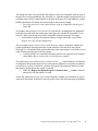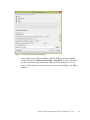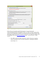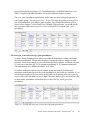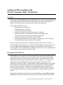
1
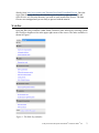
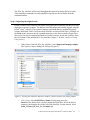
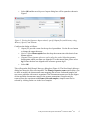
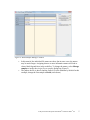
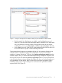
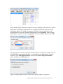
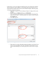
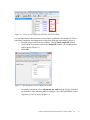
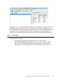
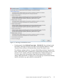
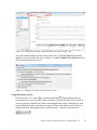
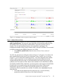
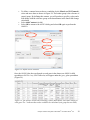
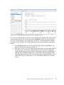
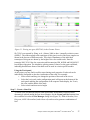
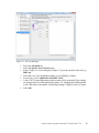
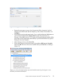
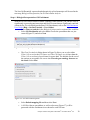
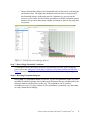
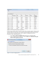
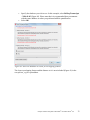
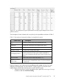
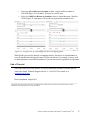
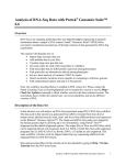
Analysis of RNA-Seq Data with
Partek® Genomics Suite® 6.6 Software
Overview
RNA-Seq is a high-throughput sequencing technology used to generate information about a
sample’s RNA content. Partek® Genomics Suite® offers convenient visualization and
analysis of the high volumes of data generated by RNA-Seq experiments.
This tutorial will illustrate how to:
• Import large next-gen data sets
• Add attribute data to your files
• Visualize large next-gen data sets
• Obtain read counts for each of the transcripts in a database
• Find transcripts that are differentially expressed among phenotypes
• Find genes that are alternatively spliced among phenotypes
• Set up a basic analysis of variance (ANOVA) model
• Detect nucleotide variations across samples or comparing to reference genome
• Find nonannotated regions and map it to the genome
Note: the workflow described below is enabled in Partek Genomics Suite version 6.6
software. Please fill out the form at www.partek.com/PartekSupport to request this version
or use the Help > Check for Updates command to check whether you have the latest
released version. The screenshots shown within this tutorial may vary across platforms and
across different versions of Partek Genomics Suite.
Description of the Data Set
In this tutorial, you will analyze an RNA-Seq experiment using the Partek Genomics Suite
software RNA-Seq workflow. The data used in this tutorial was generated from mRNA
extracted from four diverse human tissues (skeletal muscle, brain, heart, and liver) from
different donors and sequenced on the Illumina® Genome Analyzer™. The single-end
mRNA-Seq reads were mapped to the human genome (hg19), allowing up to two
mismatches, using Partek® Flow® alignment and the default alignment options. The output
files of Partek Flow are BAM files which can be imported directly into Partek Genomics
Suite 6.6 software. BAM or SAM files from other alignment programs like ELAND
(CASAVA), Bowtie, BWA, or TopHat are also supported. This same workflow will also
work for aligned reads from any sequencing platform in the (aligned) BAM or SAM file
formats.
Data and associated files for this tutorial can be downloaded by going to Help > On-line
Tutorials from the Partek Genomics Suite main menu. The data can also be downloaded
Analysis of RNA-Seq Data with Partek® Genomics Suite® 6.6
1
directly from: http://www.partek.com/Tutorials/NextGen/4TissueBamFiles.zip. Once the
zipped data directory has been downloaded to your local drive, right click the file and
select Extract All. Select the directory you wish to work in and select Extract. The data
files are now unzipped and you are ready to proceed with the tutorial.
Workflow
Open the RNA-Seq workflow within Partek Genomics Suite software by selecting it from
the Workflow drop-down list in the upper right corner of the screen. The entire workflow is
shown in Figure 1.
Figure 1: The RNA-Seq workflow
Analysis of RNA-Seq Data with Partek® Genomics Suite® 6.6
2
The RNA-Seq workflow will be used throughout this tutorial to analyze RNA-Seq data.
These and other commands for analyzing RNA-Seq data are also available from the
command toolbar.
Step 1- Importing the aligned reads
Partek Genomics Suite software can import next generation sequencing data that is already
aligned to a reference genome. The data used for this tutorial was already aligned using the
Partek® Flow® software. The sequence importer can handle the two standard alignment
formats .BAM and .SAM. Conversion from ELAND .txt files to BAM files is available via
the Tools menu. Also note that if a quantification project has been created in Partek Flow,
this project can also be imported and analyzed; in this scenario, invoke the workflow from
the very bottom of the standard RNA-Seq workflow (Figure 1: Related: Analyze a Partek
Flow project).
•
Under Import from the RNA-Seq workflow, select Import and manage samples.
The Sequence Import dialog box will open (Figure 2)
Figure 2: Viewing the Sequence Importer window. Choose the files you want to import
•
Files of type: Select BAM Files (*.bam) from the drop-down list.
Browse to the folder where you have stored the BAM files. Select the files to
import by checking the box to the left of the data files. For this tutorial, select
brain_fa, heart_fa, liver_fa, and muscle_fa
Analysis of RNA-Seq Data with Partek® Genomics Suite® 6.6
3
•
Select OK and the next Sequence Import dialog box will be opened as shown in
Figure 3
Figure 3: Viewing the Sequence Import wizard; specify Output file (and directory using
Browse), Species, and Genome
Configure the dialog as follows:
• Output file: provide a name for the top-level spreadsheet. Use the Browse button
to change the output directory
• Species: Select Homo sapiens from the drop-down menu since this data is from
human subjects
• Genome/Transcriptome reference used to align the reads: Select the genome
build against which your data was aligned to. For this tutorial data, please select
hg 19 since the data was aligned to the reference genome hg19
• Select OK
This will open the BAM Sample Manager dialog box (Figure 4). The Bam Sample Manager
dialog box shows the files to be imported. The Manage sequence names option allows you
to check or modify the chromosome name mapping (not an issue for human samples but
may cause problems with esoteric organisms if the chromosome names used by the aligner
do not match the chromosome names in the genome annotations). Samples may be
removed from the experiment with Remove selected samples; samples must first be
selected by clicking on the row in the list of samples.
Analysis of RNA-Seq Data with Partek® Genomics Suite® 6.6
4
Figure 4: BAM Sample Manager window
•
•
In this tutorial, the individual file names are short, but in some cases, the names
may be much longer. Assigning shorter or more informative names will lead to
clearer labels/legends later in the workflow, To change the names, select Manage
samples to invoke the Assign files to samples dialog box (Figure 5)
The path to the file is shown, and the Sample ID is the filename by default. In this
example, change the first sample to Brain (circled area)
Analysis of RNA-Seq Data with Partek® Genomics Suite® 6.6
5
Figure 5: Using the Assign files to samples dialog to give informative sample names
•
•
For this tutorial, the default names are suitable, so select Cancel to proceed.
However, if you have data from one sample which is split into two or more BAM
files, you can also use Manage samples to merge these reads into one sample.
Additionally, you may use Add samples or Remove selected samples if needed
Select Close to proceed. If the files are being imported for the first time, they will
be sorted in order to quickly visualize and analyze the data
The imported data will appear in a spreadsheet (Figure 6). Each sample is listed in a row
with the number of alignments displayed for each sample. You may wish to add the
samples to a separate experiment. To do so, select Import and manage samples from the
workflow again. There, you will see the BAM Sample Manager dialog box (Figure 4), but
this time there will be an additional Add new experiment button. If you press this button,
you will see the Sequence Import dialogue box (Figure 2), where you can add samples to a
new spreadsheet. For this tutorial, there is no need to create a new experiment, so press
Cancel on in the Sequence Import dialogue box and return to the spreadsheet with the
imported BAM files (Figure 6).
Analysis of RNA-Seq Data with Partek® Genomics Suite® 6.6
6
Figure 6: Viewing the imported data in a spreadsheet
Notice that the Sample ID names in column 1 are gray, denoting a text field, but we want to
change these such that the sample names are a categorical factor that can be used in the
downstream analysis. To change the properties of column 1, please right-click on the
column header to invoke the contextual menu and then select Properties. In the resulting
dialog (Figure 7), please set Type to categorical, Attribute to factor, and then select OK.
Figure 7: Setting column properties
The sample names in column 1 will now be black to denote a categorical variable. Next, we
will add attributes for grouping the data, i.e., into replicates or sample groups. From the
workflow, select Add sample attribute, then select the Add a categorical attribute
option, and then select OK (Figure 8)
Figure 8: Adding sample attributes to describe or group samples by categories
Analysis of RNA-Seq Data with Partek® Genomics Suite® 6.6
7
In this tutorial, we have four samples from different tissues, but to illustrate the statistical
analysis options later in the workflow, we will group the tissues into two groups: muscle
(muscle and heart samples) and NOT muscle (liver and brain samples). These two groups
will then be compared at a later step.
• In the Create categorical attribute dialog box (Figure 9), change Attribute name
to Tissue
• Rename Group_1 to Muscle and Group_2 to NOT muscle
• Select and drag the samples from the Unassigned box to the correct group. The
setup is shown in Figure 9. Additional groups can be added as required using the
New Group button
• Select OK to proceed
Figure 9: Create categorical attribute
•
When asked if you wish to add another categorical attribute, select No, and if you
wish to save the spreadsheet, select Yes. The attribute will now appear as a new
column with the heading Tissue and the groups Muscle and NOT muscle (Figure
10)
Analysis of RNA-Seq Data with Partek® Genomics Suite® 6.6
8
Figure 10: Tissue, a new categorical attribute, has been added
It is also important to ensure that the correct column is defined as the Sample ID. This is
particularly important when integration of data from different experiments is desired.
• From the Import section of the workflow, select Choose sample ID column
• Use the drop-down menu to select the Sample ID column; the samples names
will be shown (Figure 11)
• Select OK
Figure 11: Specifying the correct Sample ID column
•
For quality assessment, select Alignments per read from the QA/QC portion of
the workflow. After analyzing the four samples, a new child spreadsheet named
Alignment_Counts is created (Figure 12)
Analysis of RNA-Seq Data with Partek® Genomics Suite® 6.6
9
Figure 12: Alignment_Counts spreadsheet
In column 3, one can see that all imported aligned reads from Figure 6 align exactly once to
the human genome. This is dependent on the options used during the alignment process.
For other data and alignment options, one might observe more than one alignment per read.
In column 2, there are single-end reads with zero alignments per read reported because
BAM files also contain all the reads that were not aligned during the alignment process.
Step 2 – Visualization
Once imported, it is possible to visualize the mapped reads along with gene annotation
information and cytobands.
• Select the parent spreadsheet (MyRNASeqProject in this example)
• Select Plot Chromosome View in the Visualization section of the workflow.
Unless you have previously downloaded an annotation file (during another
experiment), you will be prompted to select an annotation source (Figure 13)
Analysis of RNA-Seq Data with Partek® Genomics Suite® 6.6
10
Figure 13: Selecting an annotation source
•
For this tutorial, select RefSeq Transcripts – 2014-01-03 (Note: the date beside
the RefSeq Transcripts tells the release date of the annotation database). Partek
Genomics Suite software will download the relevant file (subject to any
firewall/proxy settings) and save it to your default library location. You may also
notice a dialog flash as the cytoband file is automatically downloaded. The Partek
Genome Viewer window will open with chromosome 1 displayed (Figure 14).
You may choose other chromosomes from the drop-down menu (circled) to
change which chromosome is displayed. You may also type a search term directly
into the circled box (e.g. gene symbol or transcript ID).
Analysis of RNA-Seq Data with Partek® Genomics Suite® 6.6
11
Figure 14: Visualizing reads on a chromosome level in the Genome View
The panel on the left shows the ten tracks in the viewer. The New Track button allows
addition of a new track into the viewer (Figure 15), and the Remove Track button removes
the selected track from the viewer.
Figure 15: Adding a new track to the Genome Viewer
Using the Genome Viewer
In the Genome Viewer, select
for selection mode and
for navigation mode. In
navigation mode, to zoom in on a region of interest, left-click and draw a box to zoom in
on any region for a detailed view of the reads mapped to this region. Alternatively, in the
bottom right-hand corner of the browser, drag the slider left-to-right or click the plus (+)
button to zoom in. Drag right-to-left or click the minus (-) button to zoom back out.
Analysis of RNA-Seq Data with Partek® Genomics Suite® 6.6
12
It is also possible to zoom directly to a specific gene of interest using Partek Genome
Viewer. For example, type MYC into the search box at the top of the window, and the
viewer will show just the MYC gene in the RefSeq track and the aligned reads (Figure 16).
To return to the whole chromosome view, simply select
.
The following is a detailed description of each track in the default view.
RefSeq Transcripts (+)
The RefSeq Transcripts (+) track shows all genes encoded on the forward strand of
chromosome 1. This experiment uses RefSeqGene, which defines genomic sequences of
well-characterized genes, to be used as the reference annotation track. Mouse-over a
particular region in this track, and all genes within this region are shown in the information
bar (visible in the top right of Figure 14). Zoom into this track to see individual genes,
including alternative isoforms. Zooming in on one track automatically zooms all other
visible tracks, thus you can now see the reads that mapped to this particular gene across all
samples.
RefSeq Transcripts (-)
The RefSeq Transcripts (-) track shows all the genes encoded on the reverse strand of
chromosome 1.
Legend: Base Colors
This track indicates the color coding for individual bases. Although included in the default
view, the individual bases are only visible once zoomed into a region of interest.
Bam Profile (muscle_fa, brain_fa, heart_fa, and liver_fa)
These tracks show all the reads that mapped to chromosome one from the four tissue
samples. The y-axis numbers on the left side of the tracks indicate the raw read counts. The
aligned reads are shown in the Genome Viewer in each track with a different color for each
Bam Profile track.
Genome Sequence, Cytoband and Genomic Label
The Genome Sequence, Cytoband and Genomic Label tracks are shown at the bottom of the
panel. Genome Sequence will display the bases (different colors and labels) of the reference
genome specified when zoomed in sufficiently. The other two labels are helpful for
navigating about the chromosome.
Analysis of RNA-Seq Data with Partek® Genomics Suite® 6.6
13
Figure 16: Zooming to look at a gene of interest (MYC)
Step 3 - Analyze Known Genes
The next step in the workflow is to detect differentially expressed genes by performing
mRNA quantification. This function creates data tables at the transcript and gene levels
and identifies those transcripts that are differentially expressed or spliced across all
samples. The raw and normalized reads are also reported for each sample. The
normalization method used by Partek Genomics Suite is Reads Per Kilobase of exon model
per Million mapped reads (RPKM) (Mortazavi et al. 2008).
• Select mRNA quantification from the Analyze Known Genes section of
workflow
The RNA-Seq Quantification dialog box shown in Figure 17 will appear. Your choices for
these options depend on the aims of your experiment. In the Configure the test section
(Figure 17), you are asked about Strand-specificity. Your answer depends on the method
used for sample preparation as some methods preserve the strand information of the
original transcript and some do not. A directional mRNA-Seq sample prep protocol only
synthesizes the first strand of cDNA whereas other methods reverse transcribe the mRNA
into double-stranded cDNA. In the latter case, the sequencer reads sequences from both the
forward and reverse strands but does not discriminate between them. When strand
information is preserved, it is possible for paired-end sequences to come from a
combination of the forward and reverse strands. If in doubt, select Auto-detect from the
drop-down list.
• Select No from the Strand-specificity drop-down list, because the library
preparation method did not preserve the strand information
Analysis of RNA-Seq Data with Partek® Genomics Suite® 6.6
14
The dialog also asks if you would like the intronic reads to be compatible with the gene in
the gene-level result spreadsheets. By selecting Yes, reads that might correspond to new or
extended exons will be considered part of the gene in the gene-level spreadsheets, and the
RPKM calculation will include the intron length in the transcript length.
• For In the gene-level result report intronic reads as compatible with the gene?,
select No
You might want to Require strict paired-end compatibility, meaning that two alignments
from the same read must map to the same transcript to be considered compatible. If you
select No, then a paired-end read will be compatible with any transcript it overlaps.
• As the data set used for this tutorial consists of single-end reads, select No for
Require strict paired-end compatibility.
The next option Report results with no reads from any sample? determines whether the
results spreadsheets include transcripts or genes that have no reads from any sample.
Selecting Yes will include all the genes/transcripts in the transcriptome even if there are no
reads for that transcript/gene from any sample.
• As this tutorial is not concerned with genes that are not expressed in all samples,
select No for Report results with no reads from any sample?
The option Report unexplained regions with more than ___ reads determines if reads that
are mapped to the genome but not to any transcript are reported on a separate spreadsheet
(unexplained_regions). If checked, you must also specify the minimum number of reads
that must be present before the region is reported.
• Make sure Report unexplained regions with more than ___ reads is checked
and specify 5 as the number of reads
Lastly, the option Report exon-level results determines whether you would like to get the
exon-level expression. If checked, you will get the exon.reads and exon.rpkm spreadsheet.
Analysis of RNA-Seq Data with Partek® Genomics Suite® 6.6
15
Figure 17: RNA-Seq Quantification options
•
In this tutorial, you will use an mRNA database, RefSeq. Expand the mRNA
section and then select RefSeq Transcripts – 2014-01-03. If you would like to
get the exon-level results, please ensure that you check the Report exon-level
results. In this tutorial, we select to report exon-level results (Figure 18). OK to
continue
Analysis of RNA-Seq Data with Partek® Genomics Suite® 6.6
16
Figure 18: Specifying a transcriptome database
Reads will now be assigned to individual transcripts of a gene based on the
Expectation/Maximization (E/M) algorithm (Xing, et al. 2006). In Partek Genomics Suite
software, the E/M algorithm is modified to accept paired-end reads, junction aligned reads,
and multiple aligned reads if these are present in your data. For a detailed description of the
E/M algorithm, refer to the RNA-Seq white paper (Help > On-line Tutorials > White
Papers).
•
Select OK to perform the RNA-Seq analysis, which will generate a mapping
summary spreadsheet and several other spreadsheets containing the analyzed
results (Figure 19)
Analysis of RNA-Seq Data with Partek® Genomics Suite® 6.6
17
Figure 19: Viewing the list of results spreadsheets after detecting differential expression
and alternative splicing
The same dialog box that appears if you select Describe results will pop-up if you have not
previously turned this off. This dialog box explains the spreadsheets generated by mRNA
quantification.
The mapping_summary spreadsheet
The mapping_summary spreadsheet (Figure 20) is a summary of reads that have been
mapped to the intronic, exonic or intergenic regions. This is a QA/QC step to give you a
brief idea of how the reads are distributed across the transcriptome. You should expect the
results of replicates to resemble each other with respect to the distribution of reads.
Figure 20: Viewing the RNA-Seq_results.read.summary spreadsheet
The gene_reads and gene_rpkm spreadsheets
Partek Genomics Suite software presents the gene-level data both before (reads) and after
(RPKM) normalization. Samples are listed one per row with the normalized counts of the
reads mapped to the genes in columns. As shown in Figure 21, you can see that there are
19,969 columns representing 19,966 genes. If you see a different number of
columns/genes, this is because a different annotation database was selected in the RNA-Seq
Analysis of RNA-Seq Data with Partek® Genomics Suite® 6.6
18
Quantification dialog box (Figure 18). The normalization is by RPKM (Mortazavi, et al.
2008). Using different mRNA database will result in different number of genes.
The gene_rpkm spreadsheet is particularly useful when you have biological replicates in
your sample groups. You may go to View > Scatter Plot from the toolbar to create a PCA
plot and examine how your samples group together. For a detailed introduction of PCA,
please refer to Chapter 7 of the Partek User’s Manual. With replicates, you would also be
able to perform Differential expression analysis using ANOVA with the gene_rpkm
spreadsheet.
Figure 21: Viewing the RNA-Seq_result.gene.rpkm spreadsheet
The transcript_reads and transcript_rpkm spreadsheets
As above, Partek Genomics Suite software presents the transcript-level data both before
and after normalization. The normalized count of sequencing reads are mapped to each
transcript, listed as one sample per row with transcript IDs in columns. As shown in Figure
22, you can see that there are 39,542 columns representing 39,539 annotated transcripts.
The normalization is by RPKM (Mortazavi, et al. 2008).
If you have biological replicates in your sample groups and want to do differential
expression on the transcript level, this is the spreadsheet to you would use. Similarly, if you
have biological replicates in your sample groups and want to perform Alternative splicing
analysis, this is the spreadsheet to use as input. The same analysis (PCA and ANOVA) can
be done on this spreadsheet as described above in the RNA-Seq_result.gene.rpkm
spreadsheet.
Figure 22: Viewing the RNA-Seq_result.transcript.rpkm spreadsheet
Analysis of RNA-Seq Data with Partek® Genomics Suite® 6.6
19
The exon_reads and exon_rpkm spreadsheets
Further level of detail is to take a look at the exon-level data, presented as raw and
normalized (using RPKM), just like the gene-level and the transcript-level data. The
normalized count of sequencing reads are mapped to each exon, listed as one sample per
row with transcript IDs in columns. As shown in Figure 23, you can see that there are
244,532 columns representing 244,529 annotated exons.
If you have biological replicates in your sample groups and want to do differential
expression on the exon level, this is the spreadsheet to you would use. The same analysis
(PCA and ANOVA) can be done on this spreadsheet as described above in the RNASeq_result.gene.rpkm spreadsheet.
Figure 23: Viewing the RNA-Seq_result.exon.rpkm spreadsheet
The transcripts spreadsheet
The transcripts spreadsheet details the analysis results of RNA-Seq if there no replicates
(Figure 24 and Figure 25). Each row lists a separate transcript. A description of each
column can be found in Table 1.
Analysis of RNA-Seq Data with Partek® Genomics Suite® 6.6
20
Table 1: Column Descriptions in the transcripts spreadsheet
Column Label
Chromosome, Start, Stop
Strand, Transcript, Gene
chisq and p-value (DiffExpr)
chisq and p-value (AltSplice)
Transcript Length
Read counts (raw) of each
sample
Read counts (RPKM) of each
sample
Junction RPKM
Incompatible RPKM
Description
Genomic location of the transcript
Information about the transcript and gene symbol; + and indicate the transcript is transcribed from the forward or
reverse strand, respectively; transcript name is determined by
the transcriptome database selected (NCBI mRNA ID in this
case)
In the absence of replicates, differences in expression between
samples are detected using a log-likelihood test at the transcript
level. To sort by ascending p-value, right click the column
header and select Sort Ascending. This will show the most
significant differentially-expressed transcript at the top of the
spreadsheet
In the absence of replicates, splice-variants are detected using a
Pearson chi-square test at the gene level. Sorted by ascending
p-value shows genes with the greatest probability of expressing
different RNA isoforms between samples at the top of the
spreadsheet
Length of transcript in base pairs (bp)
Number of reads directly from the aligned data assigned to the
transcript for each sample
Raw read counts normalized by RPKM (Mortazavi, et al. 2008)
assigned to the transcript for each sample
If the aligner that was used to align this data supported junction
reads, these columns (one per sample) will show the
normalized RPKM reads assigned to junction reads for this
transcript
Paired reads only; normalized unique paired reads (RPKM)
that intersect with the transcript but are considered
incompatible because the mate is not found in the same
transcript
Figure 24: Viewing the first part of the RNA-Seq_result.transcripts spreadsheet
Analysis of RNA-Seq Data with Partek® Genomics Suite® 6.6
21
Figure 25: Viewing the second part of the RNA-Seq_result.transcripts spreadsheet
It is possible to derive basic information about differential and alternative splicing between
your samples if you don’t have replicates from the RNA-Seq_result.transcripts spreadsheet
using a simple chi-squared or log-likelihood tests since each sample is represented only
once and the null hypothesis is that the transcripts are evenly distributed across all samples.
However, the power of Partek Genomics Suite software resides in the implementation of a
mixed-model ANOVA that can handle unbalanced and incomplete datasets, nested designs,
numerical and categorical variables, any number of factors, and flexible linear contrasts
when you do have biological replicates.
Detecting differential expression using the Partek® ANOVA
During import, you created a categorical attribute called Tissue and assigned the 4 samples
to either the Muscle or NOT muscle groups. This step was to create replicates within a
group, albeit this grouping is somewhat artificial and is used in this dataset simply to
illustrate the ANOVA. Replicates are a prerequisite for analysis of differential expression
using the ANOVA test.
• Select Differential expression analysis from the Analyze Known Genes section
of the workflow. You have the choice of analyzing at either the Gene- or
Transcript-level. Select Gene-level analysis (Figure 26)
• Make sure the gene_rpkm spreadsheet is selected as the Spreadsheet
• Select OK to open the ANOVA dialog box
Analysis of RNA-Seq Data with Partek® Genomics Suite® 6.6
22
Figure 26: Differential expression analysis
•
Available factors are listed in the Experimental Factor(s) panel on the left. Move
Tissue to the ANOVA Factor(s) pane on the right as shown in Figure 27
Figure 27: The ANOVA dialog
If the ANOVA were now performed (without contrasts), a p-value for differential
expression would be calculated but would only indicate if there are differences within the
factor Tissue; it will not inform you which groups are different or give any information on
the magnitude of the change between groups (fold-change or ratio). To get this more
specific information, you need to define linear contrasts.
• Select the Contrast button (circled in Figure 27)
• For Select Factor/Interaction, Tissue will be the only factor available as it was
the only factor included in the ANOVA model in the previous step; if multiple
factors were included, they could be selected here (top red circle)
Analysis of RNA-Seq Data with Partek® Genomics Suite® 6.6
23
•
•
•
To define a contrast between the two candidate levels (Muscle and NOT muscle),
select and move them as shown in Figure 28. The bottom group is the reference or
control group. By defining this contrast, you will produce a specific p-value and a
fold change with the reference group as the denominator in the linear fold-change
calculation
Select Add Contrast (circled)
Select OK to return to the ANOVA dialog and select OK again to perform the
ANOVA
Figure 28: Define linear contrasts
Once the ANOVA has been performed on each gene in the dataset, an ANOVA child
spreadsheet ANOVA-1way (ANOVAResults) will appear under the gene_rpkm spreadsheet
(Figure 29).
Figure 29: The ANOVA results sheet showing p-value, Mean Ratio, and Fold Change for
each gene. The ? indicates that values could not be calculated (one group has no reads)
Analysis of RNA-Seq Data with Partek® Genomics Suite® 6.6
24
The format of the ANOVA spreadsheet is similar for all workflows. The description of
each column may be found in Table 2.
Table 2: Interpretation of ANOVA results
Column Label
Description
Column #
The column number in the gene_rpkm spreadsheet
Column ID & Gene Symbol
Gene Symbol based on the annotation file used
p-value (Tissue)
The overall p-value for the Tissue factor included in the ANOVA model
p-value (Muscle vs. NOT
muscle)
The specific p-value for the linear contrast of candidate levels within the factor
(in this example there are only two levels)
Mean Ratio
FoldChange and
FoldChange Description
The ratio of the mean values of RPKMs of the two groups selected in the
contrast where Group_2 is the denominator (reference); numbers less than one
imply down-regulation
Linear fold change (with 0 indicating NO change, negative numbers indicating
down-regulation, and positive numbers indicating up-regulation) for each
contrast defined and a text description
F(Tissue)
The F-statistic (essentially the ratio of signal-to-noise; high F-value = low pvalue) for each factor
SS(Tissue)
The sum of squares for each factor (rough estimate of variability within the
groups)
SS(Error) and F(Error)
Error is the variability in the data not explained by the factors included in the
ANOVA (noise). The F-value is always set to 1 (ratio of noise-to-noise)
Note that in this tutorial, the overall p-value for the factor (column 4) is the same as the pvalue for the linear contrast (column 5) as there are only two levels within factor. If we had
more than two groups, the overall p-value and the linear contrast p-values would most
likely differ. You can also see the ? symbol in the ratio/fold-change columns (6 and 7) for
several genes that also have a low p-value, resulting from zero reads in one of the groups,
thus ratios and fold-changes cannot be calculated.
For more detailed examples of setting up the ANOVA including multiple factors and linear
contrasts, please refer to the gene expression tutorials (Down’s Syndrome and Breast
Cancer) available from Help > On-line Tutorials.
The unexplained_regions spreadsheet
The contents of this sheet will be explained in more detail in Step 8.
Step 4 – Use the Genome Browser
•
Select the transcripts spreadsheet and then select Plot Chromosome View under
the Visualization tab to view the analyzed results in Partek (Figure 30)
Analysis of RNA-Seq Data with Partek® Genomics Suite® 6.6
25
Figure 30: Viewing the transcript results in the Genome Viewer
The viewer is almost identical to that seen after importing the aligned reads; the difference
is the inclusion of the Isoform Proportions track (highlighted in the Tracks list in Figure
30). Next, you are going to view a single gene, SLC25A3, to understand how the Partek
Genomics Viewer can help you visualize differential expression and alternative splicing
results.
• Type SLC25A3 in the Search bar at the top of the window and hit Enter. The
browser will browse to the gene (Figure 31)
• The muscle, brain, heart, liver, and genomic label tracks were described earlier in
the tutorial. Here, the focus is on the Isoform Proportion track to explain how
those color-coded tracks help to visualize differential expression and alternative
splicing. The reads that are mapped to a certain tissue and the proportion of the
transcript expressed in this tissue are colored the same. In this screenshot, brain is
colored red, heart is colored green, liver is colored blue, and muscle is colored
brown
Analysis of RNA-Seq Data with Partek® Genomics Suite® 6.6
26
Figure 31: Viewing one gene (SLC25A3) in the Genome Viewer
SLC25A3 was reported by Wang, et al., (Nature, 2008) to have “mutually exclusive exons
(MXEs)”. The reads mapped to the transcripts of this gene in each of the tissue samples are
shown in the browser as different tracks. The relative abundances of the individual
transcripts of this gene are shown by the height of the color coded tracks. Note the
transcript NM_213611 has low expression while transcripts NM_005888 and NM_002635
have higher expression. The alternative splicing pattern is shown, as the paper explained,
indicating that different forms of the third exon are used in a tissue-specific manner.
Using the Track panel
At this point, you may find it useful to start altering track properties. Each track can be
individually configured to alter the visualization of the reads. For example:
• Select a track and drag it to change the position of the track in the viewer
• Select the brain track, and a configuration panel will appear at the bottom of the
track panel enabling the configuration of the sequence reads display, the Y-axis,
the color, and the labels of the track
• Select a track and increase its height
Step 5 – Create a Gene List
To create a list of transcripts that are both significantly differentially expressed AND
alternatively-spliced among the four tissue samples, use the Create gene list function from
the workflow to invoke the List Manager dialog box (Figure 32). Each of the tabs (Venn
Diagram, ANOVA Streamlined, and Advanced) can be used to generate combinations of
lists.
Analysis of RNA-Seq Data with Partek® Genomics Suite® 6.6
27
Figure 32: The List Manager
•
•
•
•
•
•
•
Select the Advanced tab
Select the Specify New Criteria button
In the Configure Criteria dialog box (Figure 33), provide a name for the list (e.g.,
Diff Exp)
Select the transcripts spreadsheet and the p-value(DiffExp) column
Set Include p-values significant with FDR of 0.05
A list of 30,305 transcripts that pass this criteria will be generated. If the settings
are changed, this list will automatically update. Try changing the FDR threshold
to 0.01 and observe the number of transcripts change. Change it back 0.05 again.
Select OK
Analysis of RNA-Seq Data with Partek® Genomics Suite® 6.6
28
Figure 33: Configure Criteria dialog box
•
•
•
•
Repeat the same steps to create a list of transcripts likely alternatively spliced
using the same FDR cutoff and the AltSplice p-value column. Please name it as
Alt Splice
Select both lists in the right panel under Criteria while holding the Ctrl button on
your keyboard and then select Intersection from the left pane of the List
Manager. Select OK. A list of 17,279 genes will be generated that includes all the
genes that are both significantly differentially expressed and alternatively spliced
among the four tissue samples
Under Manage Criteria, select Save List
Please check the box for the intersection of spreadsheet Diff exp and Alt splice
and select OK. This list will now be available when you Close the List Manager
(Figure 34)
Figure 34: A list of the differentially expressed and alternatively spliced genes is now
available for downstream analysis
Analysis of RNA-Seq Data with Partek® Genomics Suite® 6.6
29
The list of differentially expressed and alternatively spliced transcripts will be used in the
next step, Biological Interpretation, for GO Enrichment Analysis.
Step 6 - Biological Interpretation: GO Enrichment
With the GO Enrichment feature in Partek Genomics Suite software, you can take a list of
significantly expressed genes/transcripts and find GO terms that are significantly enriched
within the list. For a detailed introduction of GO Enrichment, refer to the GO Enrichment
User Guide (Help > On-line Tutorials > User Guides).
• Select Gene set analysis in the Biological Interpretation section of the workflow
• Select GO Enrichment and select Next. Choose the spreadsheet that was just
created (Figure 35) and select Next
Figure 35: Selecting the spreadsheet for GO Enrichment
•
The Gene Set Analysis dialog shown in Figure 36 allows you to select either
Fisher’s Exact test or the Chi-Square test. The Chi-Square test is faster than the
Fisher’s Exact test but is less accurate for sparse data. The defaults for the rest of
the options are acceptable. Be sure to check Invoke gene ontology browser on
the result. Select Next
Figure 36: GO Enrichment options
•
•
Select Default mapping file and then select Next
A GO-Enrichment spreadsheet, as well as a browser (Figure 37), will be
generated with the enrichment score shown for each GO term
Analysis of RNA-Seq Data with Partek® Genomics Suite® 6.6
30
•
Browse through the results to find a functional group of interest by examining the
enrichment scores. The higher the enrichment score, the more overrepresented
this functional group is in the input gene list. Alternatively, you may use the
Interactive filter on the GO-Enrichment spreadsheet to identify functional groups
that have low p-values and perhaps a higher percentage of genes in the group that
are present
Figure 37: Viewing the Gene Ontology Browser
Step 7 - Detect Single Nucleotide Variations
To learn how to detect nucleotide differences and annotate SNP calls with overlapping
genes, refer to the Analysis of Nucleotide Variations in NGS Data with Partek Genomics
Suite 6.6 tutorial using Help > On-line Tutorials > Next-Generation Sequencing.
Step 8 - Detecting Unexplained Regions
During Step 3, a spreadsheet named unexplained_regions was generated (Figure 38). This
spreadsheet contains locations where reads map to the genome but are not annotated by the
transcript database (RefSeqGene, in this case). The spreadsheet can be sorted by
descending Average Coverage (column 6). This spreadsheet is potentially very interesting
as it may contain novel findings.
Analysis of RNA-Seq Data with Partek® Genomics Suite® 6.6
31
Figure 38: The unexplained_regions spreadsheet
Partek Genomics Suite software can look for genes that overlap the regions. It locates reads
not only outside of a known gene, but also takes exon/exon information from the database
and locate reads to the intron of a gene. This is helpful for finding potential novel
transcripts, exons, sequencing biases, etc.
• Go to Tools > Find Overlapping Genes option in the command toolbar
• In the resulting dialog box (Figure 39), select Add a new column with the gene
nearest to the region and then OK
Figure 39: Find Overlapping Genes
Analysis of RNA-Seq Data with Partek® Genomics Suite® 6.6
32
•
•
Specify the database you wish to use. In this example, select RefSeq Transcripts
– 2014-01-03 (Figure 40). Please note that it is recommended that you annotate
with the same database as when you performed mRNA quantification.
Select OK
Figure 40: Select the database to search for overlapping features
The closest overlapping feature and the distance to it is now included (Figure 41) in the
unexplained_regions spreadsheet.
Analysis of RNA-Seq Data with Partek® Genomics Suite® 6.6
33
Figure 41: The unexplained_regions spreadsheet showing regions mapped to the closest
genomic features
The description of each column in the unexplained peaks spreadsheet is shown in Table 3.
Table 3: Description of annotated columns in unexplained_regions
Column Label
Description
Chromosome, Start,
Stop
Genomic location of the region containing the reads
Sample ID
Sample that contains the reads mapped to this region
Length
Length of the region (in base pairs)
Average Coverage
Average read coverage in the region
Overlapping Features
Section of the nearest gene that overlaps with the region
(intron, starts before or after a gene, region contained in a
gene, gene contained within the region, region overlaps with a
gene)
Nearest Feature
Name of the nearest feature and strand (+ or -)
Distance to Nearest
Feature (bps)
Distance of the detected region to the closest gene. If the
detected region is mapped to the intron of a gene, the distance
is shown as 0
Right-clicking on a row header and selecting Browse to Location will show the reads
mapped to the chromosome. For this tutorial, a couple of genes are selected to show
regions that are located after a known gene or in the intron of a gene.
• With the unexplained_regions spreadsheet open, right-click on Average Coverage
(column 6) and select Sort Descending
Analysis of RNA-Seq Data with Partek® Genomics Suite® 6.6
34
•
•
Select row 45 and Browse to location to show a region within an intron of
UNC45B (Figure 42, left panel). This may be a novel exon
Select row 10482 and Browse to location to show a region that starts 1 bp after
CD82 (Figure 42, right panel). This peak may represent an extended exon
Figure 42: A region view of reads mapped to non-overlapping genes
While RefSeq was used to identify overlapping features, the choice of which database to
use will depend on the biological context of your experiment. For example, you may wish
to utilize promoter or microRNA databases if you are interested in regulation of expression.
End of Tutorial
This is the end of RNA-Seq tutorial. If you need additional assistance with this data set,
contact the Partek Technical Support staff at +1-314-878-2329 or email us at
[email protected].
Date last updated: August 2015
Copyright © 2015 by Partek Incorporated. All Rights Reserved. Reproduction of this material without express written
consent from Partek Incorporated is strictly prohibited.
Analysis of RNA-Seq Data with Partek® Genomics Suite® 6.6
35
References
Mortazavi, A., Williams, B.A., McCue, K., Schaeffer, L., & Wold, B. Mapping and quantifying
mammalian transcriptomes by RNA-Seq. Nature, 2008; 5: 621-8.
Wang, E.T., Sandberg, R., Luo, S., Khrebtukova, I., Zhang, L., Mayr, C., Kingsmore, S.F.,
Schroth, G.P., & Burge, C.B. Alternative isoform regulation in human tissue transcriptomes.
Nature, 2008; 456: 470-6.
Xing Y, Yu T, Wu YN, Roy M, Kim J, Lee C: An expectation-maximization algorithm for
probalisitic reconstructions of full-length isoforms from splice graphs. Nucleic Acids Res 2006,
34: 3150-3160.
Copyright © 2015 by Partek Incorporated. All Rights Reserved. Reproduction of this material without express written
consent from Partek Incorporated is strictly prohibited.
Analysis of RNA-Seq Data with Partek® Genomics Suite® 6.6
36