Download My title - Numerical Relativity Group at UBC

FD: Finite Difference Toolkit
Arman Akbarian
Department of Physics and Astronomy
Numerical Relativity Group
University of British Columbia
Vancouver, B. C.
March, 2014
Contents
1 Introduction
2
2 Overview of Finite Difference Method
2.1 Computing the FDA Expression . . . . . . . . . . . . . . . . . . . . . . . . . . . . . . . .
2.2 Iterative Schemes for Non-Linear PDEs . . . . . . . . . . . . . . . . . . . . . . . . . . . .
2.3 Testing Facilities: Convergence and IRE . . . . . . . . . . . . . . . . . . . . . . . . . . . .
3
4
6
9
3 Semantics of FD
3.1 Parsing a PDE: Fundamental Data Type .
3.2 Coordinates . . . . . . . . . . . . . . . .
3.3 Initializing FD, Make FD, Clean FD . . .
3.4 Grid Functions Set: grid functions . .
3.5 Known Functions . . . . . . . . . . . . . .
3.6 Valid Continuous Expression, VCE . . . .
3.7 Valid Discrete Expression, VDE . . . . . .
3.8 Conversion Between VDE and VCE . . .
.
.
.
.
.
.
.
.
.
.
.
.
.
.
.
.
.
.
.
.
.
.
.
.
.
.
.
.
.
.
.
.
.
.
.
.
.
.
.
.
4 Discretizing a PDE
4.1 Performing the Finite Differencing, Gen Sten . . .
4.2 Discretization Scheme, FD table . . . . . . . . . .
4.3 Changing the FDA Scheme: FDS, Update FD Table
4.4 Accessing the FD Results: Show FD . . . . . . . . .
4.5 Defining Manual Finite Difference Operators: FD .
.
.
.
.
.
.
.
.
.
.
.
.
.
.
.
.
.
.
.
.
.
.
.
.
. . .
. . .
. .
. . .
. . .
.
.
.
.
.
.
.
.
.
.
.
.
.
.
.
.
.
.
.
.
.
.
.
.
.
.
.
.
.
.
.
.
.
.
.
.
.
.
.
.
.
.
.
.
.
.
.
.
.
.
.
.
.
.
.
.
.
.
.
.
.
.
.
.
.
.
.
.
.
.
.
.
.
.
.
.
.
.
.
.
.
.
.
.
.
.
.
.
.
.
.
.
.
.
.
.
.
.
.
.
.
.
.
.
.
.
.
.
.
.
.
.
.
.
.
.
.
.
.
.
.
.
.
.
.
.
.
.
.
.
.
.
.
.
.
.
.
.
.
.
.
.
.
.
.
.
.
.
.
.
.
.
.
.
.
.
5 Posing a PDE & Boundary Conditions over a Discrete Domain
5.1 Discrete Domain Specifier: DDS . . . . . . . . . . . . . . . . . . . . . . . . . .
5.2 Imposing Outer Boundary Conditions . . . . . . . . . . . . . . . . . . . . . .
5.3 Periodic Boundary Condition: FD Periodic . . . . . . . . . . . . . . . . . . .
5.4 Implementing Ghost Cells for Odd and Even Functions: A FD Odd, A FD Even
.
.
.
.
.
.
.
.
.
.
.
.
.
.
.
.
.
.
.
.
.
.
.
.
.
.
.
.
.
.
.
.
.
.
.
.
.
.
.
.
.
.
.
.
.
.
.
.
.
.
.
.
.
.
.
.
.
.
.
.
.
.
.
.
.
.
.
.
.
.
.
.
.
.
.
.
.
.
.
.
.
.
.
.
.
.
.
.
.
.
.
.
.
.
.
.
.
.
.
.
.
.
.
.
.
.
.
.
.
.
14
14
15
15
15
16
17
17
18
.
.
.
.
.
18
18
19
20
21
23
.
.
.
.
23
24
25
26
27
6 Solving a PDEs
30
6.1 Creating Initializer Routines: Gen Eval Code . . . . . . . . . . . . . . . . . . . . . . . . . 30
6.2 Point-wise Evaluator Routines with DDS: A Gen Eval Code . . . . . . . . . . . . . . . . . . 31
1
6.3
6.4
6.5
6.6
6.7
Creating IRE Testing Routines: Gen Res Code . . . . . . . . . . .
Creating Piece-wise Residual Evaluator Routines: A Gen Res Code
Creating Solver Routine: A Gen Solve Code . . . . . . . . . . . . .
Communicating with Parallel Computing Infrastructure . . . . . .
Example: Crank-Nicolson Implementation of Wave Equation . . .
7 List of Abbreviations
1
.
.
.
.
.
.
.
.
.
.
.
.
.
.
.
.
.
.
.
.
.
.
.
.
.
.
.
.
.
.
.
.
.
.
.
.
.
.
.
.
.
.
.
.
.
.
.
.
.
.
.
.
.
.
.
.
.
.
.
.
.
.
.
.
.
32
32
32
33
34
35
Introduction
FD is a set of Maple [1, 2] routines and definitions designed to handle various tasks in applying finite
difference techniques in solving partial differential equations (PDEs). Particularly, it is developed to
provide a methodology and a syntactic language to solve time dependent or boundary value PDEs
arising in physics. Solving a PDE involves various complications, including finding the correct finite
difference approximation (FDA) to a specific accuracy, dealing with boundary points on the discretized
numerical domain, initialization, developing testing facilities for insuring accuracy, and finally creating
routines to solve the FDA equations over the numerical domain. FD is designed to simplify these steps
while providing full control over the entire process, allowing the user to focus on the underlying physical
phenomena. Specifically, FD is not created to be a “blackbox” PDE solver, rather it provides a mixed
level of automation and user controlled definitions.
FD is still under development and was originally designed to be used in the numerical relativity
research where the computational task to numerically solve the Einstein’s equations 1 , is rather challening.
Keeping that in mind, FD was developed to deal with PDEs and differential expressions that are lengthy
(in some case thousands or tens of thousands of expressions) and are usually machine generated to avoid
human error. Therefore, FD is written in the Maple language, which provides a powerful symbolic
manipulation envirounment and unifies the process of deriving the continuum form of the PDEs, and
applying finite difference methods to create a discretized form. Furthermore, FD is built to directly
parse a given differential expression2 in its canonical continuous form 3 in Maple. This eliminates the
need for having another high-level specification to define a PDE which can be a cumbersome task for
the user, especially if the PDEs are derived from tensorial equations – such as PDEs arising in general
relativity. This prevents potential human errors in transfering the equations from the symbolic calculation
enviroument to the target “PDE solver” envirounment. In addition, FD inherits all of the capabilities of
Maple language to deal with PDEs and algebraic expressions. In particular, the user can manage their
working enviroument using Maple’s built-in data and control structures and use PDEtools package to
implement various other tasks such as coordinate transformation and checking for the consistency of the
equations.4
After posing a PDE as a set of FDA equations over a discretized domain, these equations can be
solved using FD’s default point-wise Newton-Gauss-Sidel relaxation algorithm (see Sec. 2.2) – which is a
common method in solving nonlinear time dependent PDEs. FD generates Fortran subroutines (and C
wrappers) to perform the relaxation and may be used as a rapid prototyping tool to implement various
finite difference schemes to solve a PDE. It also provides a rapid development workflow to create routines
to evaluate the residual of the given FDA expression as a diagnostic tool.
FD is capable of dealing with the boundaries of the numerical domain by providing a syntax to
specifiy the PDE or boundary conditions differently at different parts of the discetized domain. This
allows the user to impose various boundary conditions such periodic boundary conditions, asymptotic
behaviour boundary conditions or inner boundary conditions. This, particularly, is achieved in FD by
implementing an equivalent method to the ghost cell technique used in finite difference methods, and
1 A set of 10 highly complex and non-linear coupled PDEs that govern the dynamices of the curved spacetime in strongly
gravitation objects like blackholes or neutrino stars.
2 PDE, written in the from: D(f ) = 0, where D is a differential operator and f is the unknown function, would be a
special case of a differential expression that is equal to zero.
3 An expression in which derivatives are presented using Maple’s diff operator. An example of such expression is:
diff(f(t,x),t,t) - diff(f(t,x),x,x)
4 We note that GRTensor [3] Maple package is avaiable for dealing with tensorial partial differential equations and tensor
manipulation.
2
can be used to create inner boundary conditions that arise from the symmetries in the system – such as
requesting particular functions to be even or odd in specific coordinate direction.
In FD’s envirounment, specifying the finite difference scheme by the user is as simple as merely
providing the order of accuracy and limitation on the allowed grid points in the Finite Difference Molecule
(FDM). FD has a simple internal algorithm to determine the number of points required to do “forward”,
“backward” and “centered” finite differencing of a given partial differential expression with the given
accuracy. It ensures that the generated stencil expression has accuracy that is equal to the user specified
value or better. The computed stencils are all stored in an internal table and are user accessible to be
monitored for their order of accuracy and form.
Finally, FD produces Fortran routines (and C wrappers) that are parallel-ready and can be used in
the framework of a high performance computing infrastructure. This is achieved by passing boundary
flags to the routines which specify if the boundaries of the grid are between CPUs or are real physical
boundaries. FD adopts PAMR’s [4] standard in this matter, but any other parallelization framework
should also have a similar method to deal with the inner CPU boundaries. We note that the Fortran
routines generated by FD use only the basic data types of Fortran language and creating wrappers to
communicate with them from a different language should be a straightforward task. By default, FD
generates the C language wrappers which is one of the most common languages in high performance
computing.
This user manual describes all of the features mentioned above and introduces the syntax of FD for
posing a PDE as a finite difference equation with the given boundary conditions. First, two algebraic
types are defined which are the fundamental objects that FD uses to identify a finite difference expression.
These types are the building blocks that FD uses to directly translate a PDE to a discretized equation
and eventually to Fortran routines. Then, a derived Maple table is introduced that specifies the PDE
and the boundary conditions over the discretized numerical domain. Finally, we present the utilities FD
provides to choose a finite difference scheme, compute the FDA equivalent of a given PDE and create
Fortran codes to solve it. We assume that the reader has a working knowledge of Maple programming
and is familiar with the basic concepts of finite difference methods. Some of these concepts are reviewed
in Sec. 2. An experienced user may skip this section, while those who are not are encouraged to consult
the references [1, 2, 5, 6].
2
Overview of Finite Difference Method
Finite difference methods are numerical techniques to express continuum differential expressions/equations as (approximate) algebraic expressions/equations. The resulting expression is known as the Finite
Difference Approximation (FDA). An FDA for a derivative term, such as df (x)/dx, at a given point x,
is a combination of the values of the function at certain points in the vicinity of x. For instance, values
at the points {f (x), f (x + ∆x), f (x + 2∆x)} (discretized values) can be used to approximate the first
derivative of the function as:
−3f (x) + 4f (x + ∆x) − f (x + 2∆x)
df (x)
≈
,
dx
2∆x
(1)
where ∆x is the step size of the discretization. This “scheme” is called forward finite differencing,
as the discrete values are extended in positive(forward) x direction. Similarly, one can use the points
{f (x), f (x − ∆x), f (x + ∆x)} to compute the second derivative of the function,
d2 f (x)
f (x − ∆x) − 2f (x) + f (x + ∆x)
≈
.
dx2
∆x2
(2)
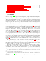
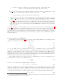
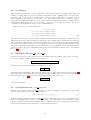
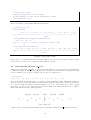
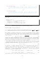
Here the point x is at the center, and thus the scheme is named centered finite differencing. The discretized points, (· · · , x − ∆x, x, x + ∆x, · · · ), construct a domain for an Ordinary Differential Equation
(ODE) or a Partial Differential Equation (PDE). The following diagram illustrates this concept of discretized numerical domain for a 1+1 (1 spatial, 1 time) dimensional spacetime:
3
fin+1
✉
✉
n
fi−1
fin
✉
✉
tn+1
n
fi+1
✉
✉
tn
✉
tn−1
fin−1
✉
✉
xi−1
xi
xi+1
A discretization method transforms a function from a continuum form to a discrete form symbolized
as:
f (t, x) → f (tn , xi ) ≡ fin .
(3)
Here, we denote the time indexing with the superscript n and the spatial indexing using the subscript
symbols (i, j, k). The grid structure, ∪xi × ∪tn , (and similarly in higher dimensions add yj and zk ) is
usually considered to be uniform:
tn = t0 + n∆t ≡ t0 + nht ,
(4)
xi = xmin + i∆x ≡ xmin + ihx ,
(5)
yj = ymin + j∆y ≡ ymin + jhy .
(6)
Using these symbols, a partial differential expression such as ∂x f (t, x) can be written as:
n
f n − fi−1
f (t, x + hx ) − f (t, x − hx )
∂f (t, x)
+ O(h2x ) = i+1
+ O(h2x ) ,
=
∂x
2hx
2hx
(7)
and the wording “approximation” is due to the neglection of the O(h2x ) term. Here the function O(h2x )
has explicit dependency of the from h2x on the step size, and represents the error of the approximation
(or equivalently can be interpretted as the “accuracy” of the FDA). Replacing all of the derivatives with
FDA expressions, a PDE becomes an algebraic equation for the discrete values of the function. For
example, consider performing the following FDA on the heat equation,
∂ 2 f (t, x)
∂f (t, x)
=0
+α
∂t
∂x2
→
n
f n − 2fin + fi−1
fin+1 − fin
+ α i+1
= 0,
ht
h2x
(8)
where in the discretized version of the equation, the unknown is the vector:
Fn+1 = fin+1 ,
(9)
and is to be solved numerically for a given Fn . Obviously knowing the values F1 , i.e the initial time
profile of the function f , the process of solving Fn+1 in terms of Fn means, by induction, finding the
entire solution on the time domain indexed by n.
2.1
Computing the FDA Expression
There is a systematic method to find the FDA of the l’th derivative of a function, dl f (x)/dxl . Consider
L points, in the vicinity of x as:
{x + q1 ∆x, x + q2 ∆x, · · · , x + qL ∆x} ,
(10)
where qi ’s are L distinct integers usually chosen in a minimalistic fashion such that x + qi ∆x is close to
x. For example, the forward and centered finite differencing in Eq. (1) and Eq. (2) are associated with:
{q1 , q2 , q3 }forward = {0, 1, 2} , {q1 , q2 , q3 }center = {−1, 0, 1} .
4
(11)
Using these L points, and L unknown coefficients {β1 , β2 , β3 , · · · , βL } one can create L Taylor expansions
upto truncation error O(∆xL ),
(L−1)
F (L−1) ,
(12)
(L−1)
F (L−1) ,
(13)
β1 f (x + q1 ∆x) = β1 F (0) + β1 q1 F (1) + β1 q12 F (2) + · · · + β1 q1l F (l) + · · · + β1 q1
β2 f (x + q2 ∆x) = β2 F (0) + β2 q2 F (1) + β2 q22 F (2) + · · · + β2 q2l F (l) + · · · + β2 q2
..
.
(L−1)
2 (2)
l
F + · · · + βL qL
F (l) + · · · + βL qL
βL f (x + qL ∆x) = βL F (0) + βL qL F (1) + βL qL
where we defined:
F (L−1) ,
dr f (x) (∆x)r
,
dxr
r!
F (r) =
(14)
(15)
and F (0) = f (x). Then we can find the coefficients {β1 , β2 , β3 , · · · , βL } such that summing over the
entire right hand sides of the equations, all of the F (r) terms have coefficients zero, except F (l) which
can be set to have coefficient 1. This process leads to the following set of L linear equations for βi ’s:
L
X
βm f (x + qm ∆x)
=
F (0)
X
βm + F (1)
m
m=1
+
···+ F
X
qm βm + F (2)
m
(l)
X
l
qm
βm
+ ··· + F
m
X
X
2
qm
βm
m
(L−1)
X
(L−1)
qm
βm = F (l)
m
βm
⇒
=0
m
X
1
qm
βm = 0
m
X
2
qm
βm = 0
m
X
l−1
qm
βm
..
.
=0
m
X
l
qm
βm = 1
m
X
l+1
qm
βm = 0
m
X
..
.
(L−1)
qm
βm = 0
m
For L distinct given qi ’s, this linear system has a unique solution vector which we denote by βi⋆ . Note
that the left hand side of the summation is a finite difference expression:
L
X
m=1
⋆
βm
f (x + qm ∆x) = F (l) =
L
l! X ⋆
dl f (x)
dl f (x) (∆x)l
=
⇒
β f (x + qm ∆x) ,
dxl
l!
dxl
(∆x)l m=1 m
(16)
and therefore we find the desired FDA expression for the l’th derivative using L neighbouring points. In
this calculation, clearly one should assume,
L ≥ l +1,
(17)
which simply indicates that finding the FDA of a l’th derivative term requires at least l + 1 points. The
truncation error in the Taylor expansions is O(∆xL ) and since the finite difference sum is divided by
∆xl in Eq. (16) the accuracy of the final finite difference expression is at least O ∆x(L−l) . However in
certain cases (for example in centered scheme) the finite difference expression can have higher accuracy
5
as the coefficient in the next leading O(∆xL ) term in the summation happens to simplify to zero. The
reader may verify this for the FDA given in Eq. (2)
This calculation is internally performed by FD as it encounters derivative terms in a PDE and returns
the FDA equivalent of them.5 There is a simple front-end function (mostly for demonstration purposes)
in FD:
Sten(diffexpr,[points])
which calls the internal FDA operator on the given differential expression, diffexpr, and computes the
stencil using the points, [points], (denoted by {qi } in the systematic derivation above). For example in
the following we demonstrate the computation of the forward and centered FDA in Eq. (1) and Eq. (2)
for the first and second derivatives respectively:
> Sten(diff(f(x),x),[0,1,2]);
-3 f(x) + 4 f(x + h) - f(x + 2 h)
1/2 --------------------------------h
> Sten(diff(f(x),x,x),[-1,0,1,2,3]);
11 f(x - h) - 20 f(x) + 4 f(x + 2 h) + 6 f(x + h) - f(x + 3 h)
1/12 -------------------------------------------------------------2
h
Example 1: Simple FDA of derivatives using FD
We emphasize that this procedure is soley for demonstration purposes, and acts only on a single derivative
term. In practice, FD uses a different procedure, Gen Sten, that performs the FDA operation according
to an FDA scheme specification provided by the user, and it performs on arbitrary length PDEs.
2.2
Iterative Schemes for Non-Linear PDEs
Solving a time dependent PDE for a function f (t, ~x) involves integrating the equation forward in time,
given the intial value f (0, ~x). In the discrete language of finite differencing, this process reduces to finding
n+1
n
the advanced time level value of the function, fijk
, for the given current value, fijk
. Starting with the
0
“intial data”, fijk
, the time integration can be performed by applying this process consecutively for Nt
time levels:
n=Nt
n=0
n=1
Initial Data fi,j,k
→ fi,j,k
→ . . . → fi,j,k
Final State
(18)
To demonstrate this update process, let’s revisit the 1-D heat equation, with a different discretization
scheme (known as leap-frog):
∂f (t, x)
∂ 2 f (t, x)
=0
+α
∂t
∂x2
→
n
f n − 2fin + fi−1
fin+1 − fin−1
+ α i+1
= 0.
2ht
h2x
(19)
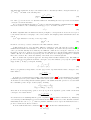
This finite difference equation (FDE), is a second order approximation to the PDE at the point (tn , xi ),
and it involves values of the function at that point, and the points in the vicinity of it. The FDE includes
the following points:
{(n + 1, i), (n − 1, i), (n, i − 1), (n, i), (n, i − 1)} .
(20)
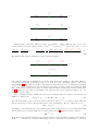
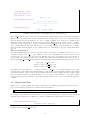
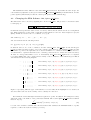
and the“unknown” in this set, as highlighted in (19), is fin+1 . This set of points is called the Finite
Difference Molecule (FDM) and is illustrated in the following diagram for the FDA of heat equation (19):
5 We
note that FD does not use any of Maple’s substituition/replacement procedures, rather it performs recursively to
parse a PDE and return FDA equivalents of its differential expressions.
6
fin+1
✈
n
fi−1
✈
✈
fin
✈
✈
tn+1
n
fi+1
✈
tn
✈
tn−1
fin−1
✈
✈
xi−1
xi
xi+1
FDM depends on the finite difference scheme. For example, consider a different (also second order
accurate) FDA of the heat equation at the point (tn+1/2 , xi ), where tn+1/2 denotes the point tn + ht /2:
!
n+1
n+1
n
n
fi+1
− 2fin+1 + fi−1
fi+1
− 2fin + fi−1
∂f (t, x)
1
∂ 2 f (t, x)
fin+1 − fin
= 0.
=0 →
+ α
+
+α
∂t
∂x2
ht
2
h2x
h2x
(21)
The FDM of this equation is illustrated in the following diagram:
n+1
fi−1
✈
fin+1
✈
n+1
fi+1
✈
tn+1
✈
tn
× tn+1/2
fin
✈
✈
xi−1
xi
xi+1
and again the unknown is highlighted both in the diagram and the equation. The main difference
between this discretization and the previus one is in the fact that, this FDM requires 2 time level,
whereas FDE (19) has 3 time levels. More importantly, in this scheme there are 3 unknowns in the FDA:
n+1
n+1
{fi−1
, fin+1 , fi+1
} and therefore there is an implicit dependency of advanced time level unknowns. This
type of FD schemes are known as implicit schemes. The FD schemes such as the leap-frog scheme used
in (19) – where the dependency of the FDM on the advanced time level is explicitly a single point – are
known as explicit schemes.
After converting a PDE to a FDE, the next step is solving this algebraic equation. We can write an
FDE in a compact form:
(22)
Lhi fin+1 , fin , · · · ≡ Lh Fn+1 , Fn , · · · = ~0 ,
where Lh is the FDA operator, the most advanced time level values, fin+1 , is considered as the unknown,
and the superscript h denotes the typical step size of the discretization. Here we defined the vector:
Fn+1 ≡ [fin+1 ] .
(23)
Depending on the PDE and the chosen FDA scheme, this equation can be solved numerically using
various methods. For a linear PDE and an explicit scheme, Eq. (22) is indeed a linear equation:
AFn+1 = b
(24)
where A is a diagonal matrix and b is a vector that depends on previous time level values of the function,
Fn , Fn−1 , · · · . In this case, solving the FDE simply reduces to inverting a diagonal matrix, i.e. inverting
7
the diagonal terms – which can be done in a single (trivial) matrix operation. But in general, if the PDE
is linear and FD scheme is implicit, the FDE reduces to the same linear euqation as (24), but the matrix
A is no longer diagonal. In even more general case, where the PDE is non-linear, and the FD scheme is
implicit, one needs to solve a non-linear algebraic equation for a vector of unknowns. Such systems are
perhpas the most interesting and are the subject of study with the FD toolkit.
In this scenario, one can solve the non-linear FDE using the multivariable iterative Netwon method:
n+1
Fn+1
− J−1 (Rl )
l+1 = Fl
(25)
in which the subsubscript l index’s the number of Newton method iterations, i.e. Fn+1
l+1 is the new
approximate solution after a single iteration, and Fn+1
is
the
old
solution.
In
recursive
Eq.
(25), J−1 is
l
h
n+1
the inverse of the Jacobian matrix of the FD operator L as a function of F
. More explicitly, it is
the multivariable derivative of the nonlinear FDA operator L:
Jji ≡
∂Lj
.
∂fin+1
(26)
Finally, in Eq. (25), l R denotes the “residual” of the FDE for the previous approximate solution generated from the Newton iteration:
Rl ≡ L Fn+1
.
(27)
l
Note that this iterative method requires an intial guess that is usually taken to be the previous time step
solution:
Fn+1
= Fn .
(28)
0
Here the logic is simple: if the PDE evolves the function slowly in time, Fn+1 is close to Fn and thus
Fn should be a good initial guess for it. Note that in this method, each time level update demonstrated
in (18) has another layer of Newton iteration presented in (25). This internal iteration usually converges
very quickly (in few steps).
So far, we have only provided a formal description of solving a non-linear FDE. Practically, the
numerical inversion of J is a non-trivial task. One can use the Gauss-Seidel or Jacobi methods to find
the inverse matrix iteratively, however, since this Jacobian is going to be used in the Newton iteration (25)
rather than performing two independet iterative schemes, one can simply find an approximate inverse
Jacobian by only taking the diagonal part of this matrix and use that in the Newton solver. 6 This
approach is called point-wise Newton Gauss-Seidel method and is equivalent to assuming that the only
unknown in FDE is fin+1 (fixing the rest of advanced time level values that occur in an implicit FDA
scheme) and solve for it using a single variable Newton method:
where:
[fin+1 ]l+1 = [fin+1 ]l − [Rii ]l /Jii
(29)
[Rii ]l = Li [fin+1 ]l
(30)
is the residual of the FDA equation at the point i and:
Jii =
∂Li fin+1 , fin , · · ·
∂fin+1
(31)
is the diagonal element of the Jacobian matrix. Note that there are two iterations involved here, one over
index i, the numerical grid, and one on the Newton iteration index l. It is ineffective to perform the l
iteration first, since a highly accurate solution to the point-wise Newton problem will become completely
n+1
disrupted as soon as the value of the next neighbouring point fi+1
is changed via the next Newton
iteration. Therefore, it is much more effective to perform the iterating over the numerical grid first. This
is known as a single point-wise Newton Gauss-Seidel relaxation sweep and if it converges, it usually only
takes few iteration. Performing this relaxation, for few times, a single time step evolution is complete
and the algorithm (18) can proceeed to the next step.
This algorithm is the first approach to solve a non-linear PDE and is the default (and at the moment
only) method that is built into FD toolkit for solving the PDEs. As we will discuss in detail, invoking
the procedure:
6 The
convergence of such method is guaranteed if the Jacobi matrix is diagnoally dominant, i.e.
8
P
i=j
|Aij | >
P
i6=j
|Aij |
A Gen Solve Code(DDS,{solve for var},input="d/c*",proc name="my proc")
will create a low level (Fortran) routine that performs the relaxation sweep. Having this routine, a PDE
can be solved by a driver routine that applies the relaxation as needed (depending on some stopping
criteria). Of course, solving a PDE involves several other steps, such as dealing with boundary points
where rather than FDA equivalent of PDE, a boundary condition needs to be imposed. This is done by
defining and passing the DDS variable which is a Maple data type to specify a PDE and its boundary
conditions over a discreized domain. It is the description of the DDS and other tools and objects that are
needed before applying this procedure that constitudes the majority of this documentation.
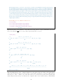
We note that a similar discussion to what we desribed about the time dependent PDEs also applies
to the boundary value problem PDE’s (elliptic PDEs). For example, consider the following second order
discretization of the Laplace equation:
fi+1,j − 2fi,j + fi−1,j
fi,j+1 − 2fi,j + fi,j−1
∂ 2 f (x, y) ∂ 2 f (x, y)
+
=0 →
+
= 0.
2
2
2
∂x
∂y
hx
h2y
(32)
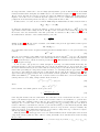
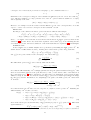
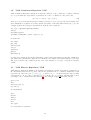
The finite difference molecule for this FDA is illustrated in the following diagram:
fi,j+1
✈
fi−1,j
✈
✈
fi,j
✈
✈
yj+1
fi+1,j
✈
yj
✈
yj−1
fi,j−1
✈
✈
xi−1
xi
xi+1
In this case, one needs to provide the discrete values of the function at the boundary points, and the
unknowns are all of the values in the interior points fij :
(BVP)
{f1,j fNx ,j fi,1 fi,Ny } → fi,j (unknown)
(33)
Again, a simple approach to solve this PDE is to use iterative schemes. For example, one can solve
the FDA equation (32) for the mid-point value fij , assuming the values at the neighbouring points are
fixed. Then performing this point-wise solver process over all of the interior points (a relaxation sweep)
iteratively will decrease the residual to the desired tolerance (if it converges). However we note that
relaxation schemes for boundary value problems (BVP) converge very slowly and other algorithms such
as multigrid [4] are essential to efficiently solve elliptic-type PDEs.
2.3
Testing Facilities: Convergence and IRE
Finding a solution to a PDE or an ODE can be a complex task. However, if the solution is given as a
discrete function, checking that it satifies the equation is somewhat a straightforward process. Consider
the equation:
L(f ) = 0 ,
(34)
where L is a differential operator and f is the unknown function. One can use an FDA scheme to
discretize the differential operator:
L → Lh
(35)
9
where h denotes the typical “size” of the discretization. Then for a given solution function, f˜, one can
evaluate the residual:
Rh = Lh (f˜)
(36)
to confirm if the function f˜ satisfies the discretized version of the equation. A solid testing facility for
a numerical solver is to independently develop this residual evaluator, which we refer as Independent
Residual Evaluator (IRE). Of course, the residual (36) will not be exactly zero since Lh is an approximation to L and perhaps f˜ is also a numerical solution to (34) that differes from the exact solution f .
However, one would expect if the solution f˜ is well resolved, is “close enough” to the exact solution,
and FDA operator Lh is a “good” approximation of L, then the norm of this residual should be orders
of magnitude smaller than the actual norm of the function f˜. A more rigorous definition of all these
concepts and how to validate the numerical solution using an IRE test will follow. However, before that
we momentarily dive into FD toolkit and how it provides a rapid workflow to creating IRE routines.
Consider the following ODE for a(x) on a given time t:
"
2 2 #
da(x) 1 − a(x)2
1
∂φ(t, x)
∂φ(t, x)
=0
(37)
+
−
− x
dx
2x
2
∂x
∂t
where φ(t, x) is a time dependent field which can have its own dynamical PDE. Here we want to evaluate
the left hand side of the equation for the given discrete solutions ai and φni and verify that it is zero
(numerically). The process involves creating an FDA of this ODE, evaluating the residual over the
numerical domain, summing up the point-wise residuals and returing a norm of it. FD toolkit provides
an almost fully automated mechanism to do so. For example, if we use FD’s default FDA scheme (second
order accurate and centered), the Maple code to generate the IRE Fortran routine in this case is:
> read "FD.mpl": Make_FD():
> grid_functions:={a,phi}:
> res_a := diff(a(x),x)/a(x) - (1 - a(x)^2)/(2*x) 1/2*x*(diff(phi(t,x),x)^2+diff(phi(t,x),t)^2):
> Gen_Res_Code(res_a,input="c",proc_name="ire_a");
Fortran Code is written to ire_a.f
C header is written to ire_a.h
C call is written to ire_a_call
Example 2: Creating testing (IRE) routines with FD is fully automated.
The steps in this examples are: loading the FD package, initializing the internal variables of FD, defining
symbols ’a’ and ’phi’ as grid functions, writing down the ODE, and passing the equation in its continuum
form to the procedure:
Gen Res Code(expr,input="c*/d",proc name="myproc");
This call creates 3 source code files:
• ire a.f: is the Fortran subroutine that evaluates the residual (37). This subroutine has the
following header:
subroutine ire_a(a,n_phi,nm1_phi,np1_phi,x,Nx,ht,hx,res)
and as you can see, it requires passing in the function a and 3 time levels of function φ, denoted by
n phi (current time), nm1 phi (retared time), and np1 phi (advanced time) since these values are
required to compute the time derivative expression in the residual (in centered scheme). The last
parameter res is a generic name, that always stores and returns the result of the computation (it
will correspond to the updated value of the dynamical function when solver routines are generated).
• ire a.h is the C header (wrapper) file that needs to be included in a C driver routine to use the
subroutine, the content of this file is:
10
void ire_a_(double *a,double *n_phi,double *nm1_phi, double *np1_phi,
double *x,int *Nx,double *ht,double *hx,double *res);
• ire a call: is a plain text file containing a typical C call of the routine. call files can be copied
to a C driver code. For example, here the content of the file is:
ire_a_(a,n_phi,nm1_phi,np1_phi,x,&Nx,&ht,&hx,res);
which as you can see, is a C call with the last parameter, again, labeled as res. After copying the
content of call to the driver code, the user needs to appropriatly change the name of the last
parameter to the allocated vector (pointer) or the single variable defined in the C driver to store the
result. 7 In this example, the result, res, is a number (a double precision floating point number)
containing the norm of the residual. FD also assumes that in the C driver, the user will define the
name of the allocated vectors and parameters for the PDE similar to what they are defined in the
Maple expression.
We will discuss this procedure and similar other code generator procedures in more details through Sec. 3
to Sec. 6. Following note is a mathematical discussion on the notion of convergence and independent
residual evaluators. Even though, these concepts are crucial to validate the consistency and accuracy of
the numerical solver, the following is somewhat independent of the FD toolkit and applies to any finite
difference method. This manual should be accessible without expertise in the mathematical discussion
in the following note.
···
Note on convergence and IRE tests
Consider that the solution in Eq.(34) is produced by solving a finite difference approximation for the
PDE. To preface this section, we first review our notation:
L(f ) = 0
(38)
S h (f h ) = 0
h
h
L (f ) = R
h
(39)
(40)
i.e. L is the PDE operator in continuum form, and f is the continuum solution, f h is the numerical
solution and S h is the solver FDA (the FDA of the original PDE that is used in the numerical solver).
Finally, Lh is another FDA to L that is different than S h , and due to this difference the RHS is nonzero
and symbolized by the residual Rh . Note that previously we used Lh to denote the FDA used in the
numerical solver, but here we are mostly interested in testing the solver using a different FDA operator
which is the main focus of this section and thus denoted by Lh .
If the numerical solution f h is convergent at the continuum limit – where the discretization size h
approaches zero– we denote the continuum limit by u:
∃u = lim f h
h→0
(41)
therefore one can assume the following Richardson expansion:
f h = u + ehf = u + e1 h + e2 h2 + · · ·
(42)
where the coefficients e1 , e2 are functions independent of h. As one might expect, the error in the
solution ehf depends on the accuracy of FDA S h that is used in the numerical solver. The first non-zero
coeffiecient ep that appears in the expansion defines the accuracy of the solution, and is the dominent
part of the error in the limit h → 0. For example, a second order convergent solution has the form:
f h = u + e 2 h2 + · · ·
(43)
7 Of course, a good strategy is to avoid naming any variables in the C driver code as res. The name res does not need
any modification in the Fortran routine or C header file.
11
and using this expansion it is easy to show that for the 3 consecutively refined convergent solutions: f h ,
f h/2 and f h/4 the limit of the following ratio:
lim Q =
h→0
||f h − f h/2 ||
= 4,
||f h/2 − f h/4 ||
(44)
is 4. Here ||.|| is some norm of a discretized functions. Measuring the factor Q is refered as standard
convergence test in the literature.
For a convergent numerical solution f h , it is not clear that the limiting continuum function u (41) is
indeed the solution to the continuum problem L(f ) = 0, i.e. we want to know if:
?
u=f.
(45)
To further emphasize this: the numerical solution f h might be convergent but we need some sort of proof
to show that it is in fact converging to the correct solution. One might speculate that this should be the
case if
1) S h approximates L correctly, or more rigorously:
lim S h = L
h→0
(46)
known as consistency condition condition for the finite difference scheme.
2) The method used to solve the finite difference equation is stable. We refer the reader to [7] for
mathematical definition and discussion on the notion of stability. In certain cases (for linear PDEs) it
can be proven that stability and consistency are sufficient conditions for convergence. However, to our
knowledege, there is no such proof for non-linear cases which most of the interesting physical systems
exhibit. We also note that from a practical point of view there is no simple prescription or condition
that can be checked off to ensure the stability of the method for non-linear systems.
Here we rather take a practical approach: the independent residual evaluation test. The IRE test
provides a stronger test than the standard convergence test, and validates (or rejects) the equality 45.
Suppose that f h is O(hp ) convergent, meaning:
f h = u + ehf
ehf = ep hp + o(hp )
(47)
where ep is a function, independent of h and o(hp ) is an h dependent function that converges to zero
faster than hp :
||o(hp )||
=0
(48)
lim
h→0
hp
Now suppose, as defined in the begining of this discussion in Eq. 40, Lh is another FDA of the original
continuum operator L (created with a different FD scheme than S h and is also created independently).
Lh is what we refer as independent residual evaluator. We assume that this operator is consistent with
the continuum operator L upto accuracy O(hq ), meaning:
Lh (g) = L(g) + ehL (g)
ehL (g) = hq EL (g) + oL (g; hq )
(49)
where EL is an h independent operator, and oL (.; hq ) is an h dependent operator with a norm that
converges to zero faster than hq :
||oL (g, hq )||
=0
(50)
lim
h→0
hq
Note that here we are assuming that the operator expansion (49) is possible for the function g. Intuitively,
one would expect this assumption to hold for functions that are well resolved over the discretized domain.
Particularly in the case of g = f h , this is a plausible assumtion, as we expect the numerical solver to
produce a well-resolved discrete solution.
Now the claim is that if the conditions (47) and (49) hold then the residual defined as:
Rh ≡ Lh (f h )
12
(51)
converges to zero if and only if f h is indeed converging to f , the contiuum solution, i.e.:
u=f
(52)
Furthermore the convergence behaviour of the residual is dominated by the two errors: the solution f h
error, which we assumed to be O(hp ) and the error of the Lh operator which we assumed to be O(hq )
and is explicitly of the form:
||Rh || = O(hp ) + O(hq ) = O(hmin(p,q) )
(53)
Therefore, for example if both the solution and the IRE are second order convergent then, one would
expect to observe a second order convergence in the residual Rh as well.
Linear case:
We first proof the claim for the linear operators L and Lh which is rather simple:
Lh (f h ) = Lh (u + ehf ) = Lh (u) + Lh (ehf ) = L(u) + ehL (u) + L(ehf ) + ehL (ehf )
= L(u) + hq EL (u) + hp L(ep ) + hq hp EL (eq ) + · · · = L(u) + O(hq ) + O(hp ) + · · ·
(54)
where · · · are higher order terms and we used the fact that L and Lh are linear operators, and from the
definition (49) ehL is also linear. Note that in the expansion of the term Lh (ehf ), we are assuming that the
error function ehf is also well resolved function on the mesh such that the expansion (49) is meaningful.
Nonlinear case:
In the nonliner case, a similar analysis can be performed by linearizing the FDA operator Lh . We
h
assume that Lh is differentiable around g, meaning there exist a linear operator DL
[g] such that:
h
Lh (g + q) = Lh (g) + DL
[g](q) + ohL [g](q)
(55)
and ohL [g] is an operator with a norm converging to zero faster than ||q||:
||ohL [g](q)||
=0
||q||
||q||→0
lim
(56)
h
The differential operator DL
[g] can be naively defined as the limit:
Lh (g + ǫq) − Lh (g)
ǫ→0
ǫ
h
DL
[g](q) ≡ lim
(57)
Note that the differentiability of Lh is simply guaranteed if all of the partial derivatives ∂Li (g)/∂g ĩ exist
where Li is the FDA equation at the point indexed by i and g ĩ is the discrete value of the function at
the point indexed by ĩ. 8 These derivatives obviously exist for normal FDA operators used in finite
h
difference methods. We also note that the abstract DL
[g] operator in a matrix representation is simply
j
the ∂Li (g)/∂g matrix. Furthermore, not surprisingly, it is equal to the FDA operator Lh itself, when
Lh is linear:
h
DL
[g](q) =
Lh (g + ǫ q) − Lh (g)
ǫLh (q)
=
= Lh (q)
ǫ
ǫ
h
h
⇒ DL
[g] = DL
= Lh
(58)
h
Note that in linear case, DL
indeed does not depend on g anymore, as the operator Lh . Assuming the
h
differentiability of L around u, we have:
h
Lh (f h ) = Lh (u + ehf ) = Lh (u) + DL
[u](ehf ) + ohL [u](ehf )
h
= L(u) + ehL (u) + DL
[u](ehf ) + ohL [u](ehf )
h
= L(u) + hq EL (u) + oL (u; hq ) + DL
[u](ep hp + o(hp )) + ohL [u](ep hp + o(hp ))
h
= L(u) + hq EL (u) + hp DL
[u](ep ) + o(hp ) + o(hp )
(59)
h
where in the last step we used the linearity of DL
[u] and the property of ohL [u] operator (56). This result
again translates to:
Lh (f h ) = L(u) + O(hp ) + O(hq ) = L(u) + O(hmin(p,q) )
(60)
8 Note
that here i and ĩ can be any of the discrete domain indecies, here we are simply using i as a symbol of discretization
13
and the residual Lh (f h ) will converge to zero, if and only if L(u) = 0, or u the continuum function that
the numerical solution f h is converging to, is indeed the underlying continuum solution f .
Now using this result we have a stronger test: The convergence of the IRE Lh (f h ) is only possible if
the solution is convergent and is converging to the corret solution. Therefore if one can create a solid IRE
operator Lh that is consistent with L, checking the convergence of the IRE will guarantee the accuracy
of the solution. Of course, one can ask: what if Lh also has an error in its implementation ? Here
the keyword independent development becomes crucial. If the independent residual is converging, it is
exteremely unlikely that S h and Lh that are developed completely independently both have an internal
error, and both of the errors agree, i.e both S h and Lh happen to be identical to an FDA for another
PDE that is not the original PDE. Often it is best to create the IRE operator Lh using an automated
process which is error-prone, this in part was the original motivation to develop FD and as it will be
discussed further, generating IRE routines is been fully automated in FD toolkit.
3
Semantics of FD
In this section, we describe some of the internal variables of FD and two derived algebraic data types
that FD uses to work with finite difference expressions.
3.1
Parsing a PDE: Fundamental Data Type
As mentioned in the introduction, FD is developed with the philosophy that user’s involvement in the
straighforward tasks should remain minimal. Consider the following PDE for f :
∂t f (t, x, z) + β(t, x, z)∂x f (t, x, z) + γ(x)∂z f (t, x, z) + a∂x2 f (t, x, z) + b∂z2 f (t, x, z) + g(x, z) = 0
(61)
The LHS written in canonical Maple form (without use of aliases) is:
PDE:=diff(f(t,x,z),t) + beta(t,x,z)*diff(f(t,x,z),x)+gamma(x)*diff(f(t,x,z),z)
+ a*diff(f(t,x,z),x,x)+b*diff(f(t,x,z),z,z) + g(x,z);
One can easily observe that this expression, by itself, contains enough information regarding the dimentionality of the problem, functions and their dependencies, parameters, and of course derivatives. By
looking at the expression, we can conclude that:
• f is a time dependent function, defined on a 2 dimenstional spatial domain labeled by (x, z).
• β is also time dependent with same spatial domain as f .
• g is a time independent function only defined on the (x, z) domain.
• γ has only 1 dimensional dependency on x coordinate.
• a and b are parameters (assuming that all dependencies are explicitly presented)
• the order and direction of derivatives of f are clear.
There is no need for further specification to pose this PDE to a computer, and the first step to reduce
potential human errors is to eliminate another syntactic language to write a PDE. Rather, FD uses
Maple’s powerful symbolic manipulation capabilities and has a built-in parser which allows directly
passing a PDE to its routines. This puts the entire complexity of the fundamental data type on the
expression, and frees the user from providing any further specification. As soon as an error-proof PDE is
written down, (which is easily possible as the working envirounment of FD is Maple with all its symbolic
tools) the task of identifying the parameters, functions, dimensionalities, derivatives, and required time
levels to perform FDA in time dimension is left to the software. This is one of the advantages of FD, over
previously developed software such as RNPL [8]. This also makes FD an efficient prototyping language,
particularly for developing testing facilities as we demonstrated in Example 2.
14
3.2
Coordinates
FD reserves the variables (t,x,y,z) for the name of the time and spatial coordinates that define the
domain of a PDE. They are protected variables after FD is loaded. Similarly, FD reserves the symbols (n,i,j,k) for indexing the corresponding coordinate points (t(n),x(i),y(j),z(k)). It uses
(ht,hx,hy,hz) as the name for the step-size of the discretization along these coordinates, respectively. The names (Nt,Nx,Ny,Nz) are reserved for the size of the discretized domain, and (xmin,xmax),
(ymin,ymax), (zmin,zmax) are reserved for flags to specify the inner CPU boundary points of the
coordinates (their applicable is in the context of parallelization).
This association can be demonestrated as:
t ↔ n ↔ ht ↔ N t
x ↔ i ↔ hx ↔ Nx ↔ (xmin, xmax)
y ↔ j ↔ hy ↔ Ny ↔ (ymin, ymax)
z ↔ k ↔ hz ↔ Nz ↔ (zmin, zmax)
(62)
and is built into FD. The coordinate names, and this association table are necessary to identify functions,
differential expressions, and perform finite differencing. For example, FD recognizes that an expression
such as f(x+hx,y-2*hy) should be discretized as f(i+1,j-2), or an expression such as f(x+hy) is invalid
and cannot be discretized, since hy is not an stepping size in x direction. Ultimately, this association table
allows FD to discretize a differential expression such as ∂x f (x, y) (in Maple notation: diff(f(x,y),x)),
directly to (f(i+1,j)-f(i-1,j))/(2*hx) without any need for further specification. (See the example
in Sec. 3.4).
3.3
Initializing FD, Make FD, Clean FD
As the reader may have noticed from the previous examples, FD is in a Maple script format, and can be
imported to a Maple worksheet/script by executing:
read("/your/fd/directory/FD.mpl");
FD’s internal variables are initialized by calling the procedure:
Make FD();
which has a short alias, MFD(), and creates the table for the coordinate association described in Eq. 62)
and initializes the default finite difference table that specifies the finite difference scheme. We will further
discuss this table in Sec 4.2. To clean the initialized variables, user can execute:
Clean FD();
or use the alias CFD().
3.4
Grid Functions Set: grid functions
FD uses a global variable named grid functions (of type set in Maple) as its reference for all of the
function names that are expected to be discretized as:
n
f (t, x, y, z) → f (tn , xi , yj , zk ) ≡ fi,j,k
.
(63)
In Maple language, if symbol f is in the grid functions, then the function f(t,x,y,z) (in its most
generic 1+3 dimenstional case) will be converted to f(n,i,j,k) during the process of discretization. The
following example demonstrates how FD uses the coordinate names, the coordinate association table,
and the symbols defined in grid functions to produce FDA expressions:
15
> read "FD.mpl": MFD():
> grid_functions:={f}:
> Gen_Sten(f(t,x,y,z));
f(n, i, j, k)
> Gen_Sten(diff(f(x,y),x));
f(i - 1, j) - f(i + 1, j)
-1/2 ------------------------hx
> Gen_Sten(x+g(y,z));
x(i) + g(y(j), z(k))
Example 3: Discretization of grid functions vs non-grid functions
Here, Gen Sten is the main routine that performs the finite differencing and will be discussed extensively.
However, user can easily guess its functionality from the example. As it can be seen, beside the names
that are included in the grid function set, the coordinate variables (t,x,y,z) are by definition grid
functions and are discretized as (t(n),x(i),y(j),z(k)). Furthermore, if a symbol with coordinate
dependency (such as g(y,z) above) is not included in the grid functions set, it will be considered
as an external function that user will provide to the Fortran routines. FD discretizes its coordinate
functions rather than the function. For example, here it is discretized as: g(y(j),z(k)) rather than
g(j,k).
Time Level Reduction:
We shall emphasize that the discrete expression f(n,i,j,k) will be eventualy (at the point of code
generation) replaced by: n f(i,j,k). This proceess is done internally, and is refered as time level
reduction (See Sec. ??). The time level n is usually refered as current time level, n-1 is refered as
retarded time level and n+1 is called advanced time level. When FD performs the time level reducion, it
uses the prefix np1 and nm1 in the names of the advance and retarded time levels functions respectively:
f(n,i,j,k) → n f(i,j,k)
f(n+1,i,j,k) → np1 f(i,j,k)
f(n-1,i,j,k) → nm1 f(i,j,k)
The higher time level f(n+2,i,...) will be renamed to np2 f(i,...) and the syntax for the other
cases should be clear. This replacement is simply because in time dependent finite difference algorithms
only a finite number of time levels are needed and stored in the memory during the time evolution. The
user can define the time levels in the C driver code according to this standard, or can define “alias”
pointers (that adopts these names) to the underlying data structure to be able to use the FD generated
routines.
3.5
Known Functions
FD has a set of “known” functions, which is basically a set of floating point functions that are known to
the low level language (Fortran here). These functions in FD are:
{ln,log,exp,sin,cos,tan,cot,tanh,coth,sinh,cosh,exp,sqrt,‘∧‘,‘*‘,‘+‘,‘-‘,‘/‘}
and during a discretization process, FD does not convert their arguments to a discrete version, rather it
discretizes the arguments accordingly. For example, sin(z)*f(x)+exp(y) will be discretized as:
> Gen_Sten(sin(z)*f(x)+exp(y));
sin(z(k)) f(i) + exp(y(j))
assuming that f is in grid functions.
16
3.6
Valid Continuous Expression, VCE
Valid Continuous Expression (VCE) is an algebraic function of the continuous coordinate variables,
(t, x, y, z), in which the dependencies of grid functions on the coordinates are only of the form:
f (t + lht , x + mhx , y + qhy , z + phz ) ,
(64)
where (l, m, q, p) are known integers (not variable), and (ht , hx , hy , hz ) are the associated stepsize variables. Furthermore, a VCE does not have explicit dependency on the discretiztion indices (n, i, j, k). For
example, if functions f and g are grid functions, then all of the exressions:
f(t,x,y) + (g(x+hx)-g(x-hx))/(2*hx)
r(x*y)
u(sin(x*y),g(z))
f(x+2*hx,y-3*hy)/hz + x*z^2 + g(z,x,t,y)
are VCE, and
f(t,x+hy)
g(x,y+2)
f(x(i),y(j))
cos(j)
f(u(x),y)
g(x*y)
diff(f(x),x)
are all invalid continuous expressions. Particulary, compare g(x*y) and r(x*y), former is not VCE, since
g is defined as a grid function, while later is a VCE as r is considered an external function. Note that
FD does not check for the consistency in the order of the variables, i. e. f(x,y) + f(y,x) is considered
a VCE.
3.7
Valid Discrete Expression, VDE
Valid Discrete Expression (VDE) is an expression in which the explicit dependencies of functions on
the discretization indecies (n,i,j,k) is only via the grid functions or coordinates. Furthermore, this
dependency is of the form: f (n + q, i + m, j + p, . . . ), where q, m, p, · · · are known integers, and f is either
a grid function or is one of the coordinates (t, x, y, z). In the case of coordinate, indexing must be done
according to the coordinate-index association (62). For example, for grid functions:={f,g}:
g(i+1,j-2)
x(i)
u(x(i),f(j,k),a)
f(j,k+2,i)
are all VDE and,
y(i)
x(i)+k
sin(i)
f(i*j)
u(i)
f(i,y(j))
are invalid discrete expression.
17
3.8
Conversion Between VDE and VCE
The definition of VDE and VCE allows a one-to-one mapping between these two types. FD provides two
functions for the conversion:
A:=DtoC(B::VDE);
B:=CtoD(A::VCE);
Even though VCE’s are not practically useful for numerical implementations, the conversion of a VDE
to VCE can be used for demonstration and testing purposes. For example, a finite difference expression
in VDE form, can be converted to a VCE, and then a taylor expansion of it can reveal its equivalent
continuum differential operator. The following demonstrates the process for Kreiss-Oliger dissipation
operator [7] that is commonly used in finite difference methods:
> read "FD.mpl": Make_FD():
> grid_functions:={f}:
> A:= -epsdis/(16*ht)*( 6*f(n,i) + f(n,i+2) + f(n,i-2)
-4*(f(n,i+1) + f(n,i-1))
):
> B:=DtoC(A):
> E:=convert(series(B,hx),polynom);
4
epsdis D[2, 2, 2, 2](f)(t, x) hx
E := -1/16 --------------------------------ht
Example 4: Conversion between VDE and VCE
which gives:
E=
4
−ǫ ∂ 4 f (t, x) h4x
)
(
16
∂x4
ht
(65)
Discretizing a PDE
In this section we discuss how to perform a finite differencing on a PDE using the facilities of FD, how
to choose a specific discretization scheme and and how to access the results of a lengthy finite difference
operation.
4.1
Performing the Finite Differencing, Gen Sten
The main routine that performs FDA is:
VDE/VCE::Gen Sten(expr)
(with an alias: GS) where the expr is an arbitrary mixed differential/algebraic Maple expression. As
mentioned before, this routine performs the discretization on the grid functions and coordinates, leaving
parameters and other functions unchanged ( the coordinate of the functions however will be discretized).
The result is by default a VDE type. To return a the finite difference expression in VCE form, the
optional input discretized should be disabled:
VCE::Gen Sten(expr,discretized=false)
Note: In the examples in the rest of this manual, we assume that the FD initialization is invoked and
f and g are grid functions:
18
> read "FD.mpl": MFD():
Warning, grid_functions is not assigned
FD table updated, see the content using SFDT() command
> grid_functions:={f,g}:
Here is an example of discretizing differential expressions:
> A:=diff(f(x,y),x,y):
> B:=Gen_Sten(A);
-f(i - 1, j - 1) + f(i - 1, j + 1) + f(i + 1, j - 1) - f(i + 1, j + 1)
B := -1/4 ---------------------------------------------------------------------hy hx
> Gen_Sten(diff(f(x),x)+g(y)+cos(f(x))+r(x)+z);
f(i - 1) - f(i + 1)
-1/2 ------------------- + g(j) + cos(f(i)) + r(x(i)) + z(k)
hx
> Gen_Sten(A,discretized=false);
-f(x - hx, y - hy) + f(x - hx, y + hy) + f(x + hx, y - hy) - f(x + hx, y + hy)
-1/4 -----------------------------------------------------------------------------hy hx
Example 5: Discretizing a PDE
As one can see, the default discretization scheme in FD is centered (and second order accurate). In the
next section, we describe how to change the finite difference scheme.
4.2
Discretization Scheme, FD table
FD uses an internal table, FD table, to perform the finite difference operations such as ones in Example
5. This table, simply is a list of the points that can be used for the n’th derivative computation for each
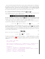
of the coordinates (t,x,y,z). For example, the x compoent of this table is:
> FD_table[x];
[[0], [-1, 0, 1], [-1, 0, 1], [-2, -1, 0, 1, 2], [-2, -1, 0, 1, 2], ...
where n’th element (counting from zero), is a list of points specifiying the finite differencing scheme for
the n’th derivative along x. The numbers present the list of neighbooring points to x(i) that are allowed
to be used for FDA. For instance, the third element, [-2,-1,0,1,2], presents the 5 points: centeral
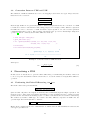
point x(i), 2 to left and 2 to right, that are allowed for FDA of the third derivatives in x coordinate.
This is demonstrated in the following diagram.
x(i-2)
×❡
...
❡
−2
x(i-1)
←
❡
−1
x(i)
↓
←
✉
x(i+1)
→
0
❡
1
x(i+2)
→
❡
...
×❡
2
[-2,-1,0,1,2]
Figure 1: Five points specifing the FDA scheme for the third derivatives in FD table in x direction.
19
FD initializes the finite difference table when Make FD() is invoked. By default, the table is upto the
5’th derivatives (adjustable by the global variable MAX DERIVATIVE NUMBER=5) in all dimensions, and the
points expand symmetrically around the central point (centered finite differencing).
4.3
Changing the FDA Scheme: FDS, Update FD Table
The FD scheme can be chosen by adjusting the content of FD table. FD provides a convenient routine
for this purpose:
Update FD Table(order::integer,fds::FDS);
in which the user specifies the desired order of accuracy, order, and the scheme via the second argument
fds. This argument is a table with a particular format which we refer as a Finite Difference Specifier
(FDS). A FDS is a table for the 4 coordinates, (t,x,y,z),
fds:=table( [ t=... , x=..., y=... , z=...] );
and each element has the following format:
X = [p_left,-1] or [-1,-1] or [-1,p_right]
in which X denotes one of the coordinates, and the values p left and p right are known integers.
p left specifies how many points to left of the central point is allowed, and similarly p right specifies
the number of points to the right that can be used in an FDA for coordinate X. If these values are set to
-1 it allows FD to expand in that direction to as many point as needed to achieve the desired accuracy.
At least one of the p-values must be set to -1. Particularly, the p left and p right need to be adjusted
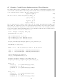
for creating FDAs that can be applied in the vicinity of the boundaries of the numerical grid. This is
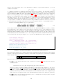
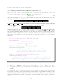
demonstrated in the following diagram:
...
❡ ❡ ❡ ❡ ✉
fds:=table([ t=[-1,-1],x=[-1,0],y=[-1,-1],z=[-1,-1] ]):
...
❡ ❡ ❡ ✉ ❡
fds:=table([ t=[-1,-1],x=[-1,1],y=[-1,-1],z=[-1,-1] ]):
...
❡ ❡ ✉ ❡ ❡
fds:=table([ t=[-1,-1],x=[-1,2],y=[-1,-1],z=[-1,-1] ]):
...
❡ ❡ ✉ ❡ ❡
...
fds:=table([ t=[-1,-1],x=[-1,-1],y=[-1,-1],z=[-1,-1] ]):
❡ ❡ ✉ ❡ ❡
...
fds:=table([ t=[-1,-1],x=[2,-1],y=[-1,-1],z=[-1,-1] ]):
❡ ✉ ❡ ❡ ❡
...
fds:=table([ t=[-1,-1],x=[1,-1],y=[-1,-1],z=[-1,-1] ]):
✉ ❡ ❡ ❡ ❡
...
fds:=table([ t=[-1,-1],x=[0,-1],y=[-1,-1],z=[-1,-1] ]):
Figure 2: Specifying different types of FD schemes: note the values in the highlighted color and how it
associates with each case at the vicinity of the boundary in x direction.
We remind the reader that higher derivatives require more points. In addition, increasing the accuracy
order also adds to the number of the points used in FDAs. The routine Update FD Table has a built-in
function P (n, m)
∂m
with O(hn ) accuracy → P (n, m)
(66)
∂X m
for each of the forward, backward and centered schemes that estimates the minimum number of points
required to achieve the desired accuracy (or better).
20
For example the following code updates the FD table use FD scheme forward in time, centered in
x, backward in y and asymetric backward in z, with 4’th order accuracy. The resulting FD table is
demonstrated by inspecting each element of it:
> fds:=table([t=[0,-1],x=[-1,-1],y=[-1,0],z=[-1,2]]):
> Update_FD_Table(4,fds):
FD table updated, see the content using SFDT() command
> FD_table[t];
[[0], [0, 1, 2, 3, 4], [0, 1, 2, 3, 4, 5, 6],...]
> FD_table[y];
[[0], [-4, -3, -2, -1, 0], [-6, -5, -4, -3, -2, -1, 0], ...]
> FD_table[z];
[[0], [-2, -1, 0, 1, 2], [-4, -3, -2, -1, 0, 1, 2], [-4, -3, -2, -1, 0, 1, 2],...]
Example 6: Changing the Finite Difference Scheme
We note that FD table can be updated manually by overwriting the elements, however this method
is error-prone, and higher derivatives in particular might not have a sufficient number of points to be
evaluated as a FDA. For example, in the following, we specify only 2 points for the second derivative in
time, and the Gen Sten procedure outputs an error as it is impossible to compute the FDA equivalent
of the input according to the FD table:
> FD_table[t]:=[[0],[0,1,2],[0,1]]:
> Gen_Sten(diff(f(t,x),t));
-f(n, i) + f(n + 1, i)
---------------------ht
> Gen_Sten(diff(f(t,x),t,t));
Error, (in Calc_Stencil_L) Failed to find FDA coefficients, check FD_table content!
Finally, we note that the entire content of FD table (rather lengthy sequence of integers!) can be viewed
using the procedure:
Show FD Table();
4.4
Accessing the FD Results: Show FD
If the Gen Sten procedure is used to perform finite differencing on a lengthy differential expression, the
resulting FDA is not human readible. To better present what Gen Sten has performed, the routine stores
the differential expressions it finds in the input and their FDA equivalent that it replaces them with, in
an internal table named FD results. The content of this table can be accessed using the procedure:
Show FD();
For example, consider the following finite differencing operation:
> A:=diff(y*f(x,y)*diff(sin(x*y)*g(x),x),x,y):
> B:=Gen_Sten(A):
memory used=11.4MB, alloc=5.4MB, time=0.59
> lprint(B);
1/2*(-f(i-1,j)+f(i+1,j))/hx*(cos(x(i)*y(j))*y(j)*g(i)-1/2*sin(x(i)*y(j))*(g(i-1)-g(i+1))
21
/hx)+1/4*y(j)*(f(i-1,j-1)-f(i-1,j+1)-f(i+1,j-1)+f(i+1,j+1))/hy/hx*(cos(x(i)*y(j))*y(j)*g
(i)-1/2*sin(x(i)*y(j))*(g(i-1)-g(i+1))/hx)+1/2*y(j)*(-f(i-1,j)+f(i+1,j))/hx*(-sin(x(i)*y
(j))*x(i)*y(j)*g(i)+cos(x(i)*y(j))*g(i)-1/2*cos(x(i)*y(j))*x(i)*(g(i-1)-g(i+1))/hx)+f(i,
j)*(-sin(x(i)*y(j))*y(j)^2*g(i)-cos(x(i)*y(j))*y(j)*(g(i-1)-g(i+1))/hx+sin(x(i)*y(j))*(g
(i-1)-2*g(i)+g(i+1))/hx^2)+1/2*y(j)*(-f(i,j-1)+f(i,j+1))/hy*(-sin(x(i)*y(j))*y(j)^2*g(i)
-cos(x(i)*y(j))*y(j)*(g(i-1)-g(i+1))/hx+sin(x(i)*y(j))*(g(i-1)-2*g(i)+g(i+1))/hx^2)+y(j)
*f(i,j)*(-cos(x(i)*y(j))*x(i)*y(j)^2*g(i)-2*sin(x(i)*y(j))*y(j)*g(i)-sin(x(i)*y(j))*x(i)
*y(j)*(-g(i-1)+g(i+1))/hx+cos(x(i)*y(j))*(-g(i-1)+g(i+1))/hx+cos(x(i)*y(j))*x(i)*(g(i-1)
-2*g(i)+g(i+1))/hx^2)
#
>
>
>
>
Checking if B is indeed an FDA for A:
E:=DtoC(B):
E:=convert(series(E,hx,4),polynom):
E:=convert(series(E,hy,4),polynom):
residual:=simplify(eval(A-E,hx=0,hy=0));
residual := 0
Expression A has several derivatives of the functions f and g that are replaced with FDA expressions.
Now by invoking Show FD() we can see what replacements have been done:
> Show_FD();
d
-f(i - 1, j) + f(i + 1, j)
{-- f(x, y) = [1/2 --------------------------, [[x, 2], [y, -1]]],
dx
hx
d
f(i, j - 1) - f(i, j + 1)
-- f(x, y) = [-1/2 -------------------------, [[y, 2], [x, -1]]],
dy
hy
d
-g(i - 1) + g(i + 1)
-- g(x) = [1/2 --------------------, [[x, 2]]],
dx
hx
2
d
g(i - 1) - 2 g(i) + g(i + 1)
--- g(x) = [----------------------------, [[x, 2]]],
2
2
dx
hx
d
g(j - 1) - g(j + 1)
d
-- g(y) = [-1/2 -------------------, [[y, 2]]], ----- f(x, y) = [
dy
hy
dy dx
-f(i - 1, j - 1) + f(i - 1, j + 1) + f(i + 1, j - 1) - f(i + 1, j + 1)
-1/4 ----------------------------------------------------------------------,
hy hx
[[x, 2], [y, 2]]] }
Here the numbers next to the coordinate variables x,y denotes the order of accuracy of the replacement,
and as expected they are all second order accurate. -1 represents exact FDA, i.e. there is no differentiation
with respect to that coordinate. Note that this accuracy is not what user specifies when updating FD
scheme (in previous section). It is indeed the computed value of the actual accuracy of FDA which
22
should be equal or higher to the user specified value.
4.5
Defining Manual Finite Difference Operators: FD
FD provides a way to define an arbitrary FDA operator. In principal, any finite difference operator can
be created from the shifting operator (See [7]) defined (in 1 dimension) as:
E(fi ) = fi+1
(67)
and its inverse is simply: E −1 (fi ) = fi−1 . The generalizaion of this operator is defined in the FD toolkit,
and is named FD with the following format:
VDE::FD(dexpr::VDE, [ [t shift] ,[x shift,y shift,z shift] ])
in which FD takes an input dexpr of type VDE, and returns a VDE that is shifted by the given integers
(t shift, x shift,y shift,z shift). If there is no time index dependency in the expression, the first
argument, [t shift], can be dropped and the routine accepts a shorter format:
FD(VDE,[x shift,y shift,z shift])
Similarly if z index k does not occur in the VDE, the routine accepts shorter list [x shift,y shift] and
so on. For example, the following demonstrates the definition of 3 manual FDA operators: 1) a forward
time derivative FDA (DT) that is equivalent to ∂t upto first order accuracy, 2) centered in x derivative
FDA (DXC), which is equivalent to ∂x upto second order accuracy, and 3) the time averaging operator
AVGT that is not an FDA. This operator is usually used in Crank-Nicolson method to create a implicit
FD scheme.
> DT := f -> ( FD(f,[[1],[0]]) - FD(f,[[0],[0]]) )/ht:
> df:= DT(f(n,i));
f(n + 1, i) - f(n, i)
df := --------------------ht
> DXC:= f -> ( FD(f,[1,0]) - FD(f,[-1,0]) ) /(2*hx):
> DXC(f(i)*x(i)^2*g(j)+y(j));
2
2
f(i + 1) x(i + 1) g(j) - f(i - 1) x(i - 1) g(j)
1/2 ------------------------------------------------hx
> AVGT := f -> ( FD(f,[[1],[0]]) + FD(f,[[0],[0]]) )/2:
> AVGT(Gen_Sten(diff(f(t,x),x)));
f(n + 1, i - 1) - f(n + 1, i + 1)
f(n, i - 1) - f(n, i + 1)
-1/4 --------------------------------- - 1/4 ------------------------hx
hx
Example 7: Defining manual dinite difference operators
5
Posing a PDE & Boundary Conditions over a Discrete Domain
In solving PDEs, it often occurs that some part of the discretized domain needs special treatment.
By its nature, boundary points require different equations than the original PDE. In adddition, if the
discretization scheme results in large finite difference molecules, the points next to the boundaries also
require special handling. For example consider 4’th order accurate FDA of the derivative of a function,
∂x f (x):
23
f(i - 2) - 8 f(i - 1) + 8 f(i + 1) - f(i + 2)
1/12 --------------------------------------------hx
This expression cannot be evaluated where i < 3 or i > Nx − 2, as the finite difference molecule
(-2,-1,0,1,2) require points that do not exist in the discretized domain at these limits. In this section,
we describe the methodology to create different equations for each part of the numerical domain, and
the facilities FD provides to impose boundary conditions and implement techniques such as ghost cells.
5.1
Discrete Domain Specifier: DDS
To specify each portion of the discrete domain, {i ∈ (1, Nx )}×{j ∈ (1, Ny )} · · · , FD uses a syntax similar
to RNPL [8], via a derived data type that we refer as Discrete Domain Specifier (DDS). A DDS is a list
of equations:
DDS = [ equation1, equation2, ...
]
where each equation specifies part of the discrete domain and has the following LHS and RHS:
each equation:
{ indexeq1, indexeq2, ...
} = expression
in which each expression can be a VDE, or a continuous PDE, and each indexeq describes the indexing
for one of the spatial dimensions:
each indexeq:
I = [start,NI-stop,step]
Here, the variable I denotes one of the indexing labels, (i,j,k), NI is the associated domain size
Nx,Ny,Nz, and step is a known integer that determines the stepping size. The indexeq symbolizes a
portion of the domain in which index I takes the values: (start,start+step,start+2*step,...) and
ends at value smaller or equal to NI-stop. The reader may notice that this is exactly equivalent to a for
loop structure. For example
{ i = [1,Nx,1] , j =[2,Ny-1,2] } = ...
is equivalent to (in Fortran syntax):
DO i=1,Nx,1
DO j=2,Ny-1,2
...
ENDDO
ENDDO
The following example clarifies this syntax, and demonstrates a DDS for heat equation where the boundary points are fixed to values T0 and T1 and interior points are specified by the heat equation.
HeatEq:= diff(f(t,x),t) - diff(f(t,x),x,x);
HeatDDS := [
{ i=[1,1,1]
} = f(n+1,i) - T0 + myzero*x(i)
{ i=[2,Nx-1,1] } = Gen_Sten(HeatEq)
{ i=[Nx,Nx,1]
} = f(n+1,i) - T1 +myzero*x(i)
];
,
,
Example 8: 1-D discrete domain specifier for the heat equation
24
The necessity of myzero*x(i) expression will become clear later when we use this DDS as an input to
FD’s solver routine generator.
Note that heat equation and its boundary conditions are simple and compact enough to be discretized
inside the DDS. For a more complex case, it is better to create the discrete version of the equations for
the boundaries seperaterly, and pass them into the DDS using human readable names. For example,
the following demonstrates a 2 dimensional DDS where each boundary uses a specific discrete equation
priorly created by the user:
mydds2d := [
# Interior points:
{ i=[2,Nx-1,1] ,
# Boundaries:
{ i=[1,1,1]
,
{ i=[Nx,Nx,1] ,
{ i=[1,Nx,1]
,
{ i=[1,Nx,1]
,
];
j = [2,Ny-1,1] } =
j = [1,Ny,1]
j=[1,Ny,1]
j=[1,1,1]
j=[Ny,Ny,1]
}
}
}
}
=
=
=
=
EQD_interior ,
EQD_left
EQD_right
EQD_bottom
EQD_top
,
,
,
Example 9: Two dimensional DDS
For a set of coupled PDEs, the user can create the FDAs and DDS’s using a Maple foor loop. Note that
FD will check for consistency of the LHS and RHS of each element of DDS as well as the consistency
between all the elements. It will raise errors if the finite difference expression on the RHS does not have
the same dimensionality as the LHS. However at the moment FD does not check if the finite difference
molecule on the RHS fits into the domain specified on the LHS. The user need to be careful with the
manual discretization of the equations, and to avoid out of range errors, it is best to use finite difference
specifiers (FDS) discussed in Sec 4.3.
5.2
Imposing Outer Boundary Conditions
The next step is to create the appropriate FDA expressions (the RHS expressions in the DDS) that are
compatible with specfic boundary conditions and also are created under consideration that there are
limitations on the allowed points in the vicinity of the boundary points. The case of fixing the value
of the function or Dirichlet boundary condition is quite simple and demonstrated in the example for
heat equation. Often other types of boundary conditions appear in physical systems. One of particular
interest is the “out-going” type or Neumann boundary condition. For a 1-D wave equation the out-going
boundary condition is given by:
∂t f (t, x) = −∂x f (t, x)
(68)
for the right side boundary i=Nx that corresponds to the approximate positive “infinity” of the numerical
domain x = +L∞ . The out-going boundary condition at the the left side of the numerical domain is
given by:
∂t f (t, x) = +∂x f (t, x)
(69)
for the point i=1 or x = −L∞ . To implement such boundary conditions, one needs to use FDA expressions that can be evaluated at the point of boundary that does not allow symmetric FD scheme.
As described in Sec. 4.3, this is achieved by changing the FDA scheme in FD using finite difference
specifiers (FDS). For example, the following demonstrates an implementation of a mixed boundary for
wave equation in which left boundary is fixed while the right boundary is outgoing. Note the change of
FDA scheme using the FDS: fds backwardx.
WaveEq := diff(f(t,x),t,t) - diff(f(t,x),x,x):
WaveEqBdy := diff(f(t,x),t) + diff(f(t,x),x):
WaveEqD := Gen_Sten(WaveEq):
25
fds_backwardx:=table([ t=[-1,-1],x=[-1,0],y=[-1,-1],z=[-1,-1] ]):
Update_FD_Table(2,fds_backwardx):
WaveEqBdyD := Gen_Sten(WaveEqBdy):
ddsWAVE:= [
i=[1,1,1]
i=[2,Nx-1,1]
i=[Nx,Nx,1]
];
= f(n+1,i) - myzero*x(i) ,
= WaveEqD,
= WaveEqBdyD
Example 10: Specifiying outgoing/mixed boundary condition for wave equation
5.3
Periodic Boundary Condition: FD Periodic
Another common boundary specficiation is peridoc boundary condition (PBC). FD provides a facility to
implement PBCs by making a VDE periodic. The procedure:
FD Periodic(exprd::VDE,{I=1/NI})
takes an input, exprd, of type VDE and creates a periodic version of it. This location is specified by the
second argument, in which I is one of the indeces (i,j,k) and the RHS is either 1 or NI where NI is
one of the associated grid size (Nx,Ny,Nz). For example i=1 denotes that a periodic version of VDE is
needed at the left boundary and i=Nx denotes the same for the right boundary point. The replacements
done on FDA is illustrated in the following graph:
F(i−1) (at i=1) replaced wtih F(i+Nx−2)
i=Nx
........
i=1
F(i+2) (at i=Nx) replaced with F(i−Nx+3)
The following example, demonstrates the effect of the FD Periodic procedure on a VDE:
> FD_table[x]:=[ [0], [-1,0,1] ,[-2,-1,0,1,2] ]:
> A:= Gen_Sten(diff(f(x),x,x));
f(i - 2) - 16 f(i - 1) + 30 f(i) - 16 f(i + 1) + f(i + 2)
A := -1/12 --------------------------------------------------------2
26
hx
> FD_Periodic(A,{i=1});
f(i - 3 + Nx) - 16 f(i - 2 + Nx) + 30 f(i) - 16 f(i + 1) + f(i + 2)
-1/12 ------------------------------------------------------------------2
hx
> FD_Periodic(A,{i=Nx});
f(i - 2) - 16 f(i - 1) + 30 f(i) - 16 f(i + 2 - Nx) + f(i + 3 - Nx)
-1/12 ------------------------------------------------------------------2
hx
Finally, using this procedure, the implementation of a periodic DDS for wave equation can be achieved
as following:
ddsWAVE_Periodic:= [
{ i=[1,1,1]
} = FD_Periodic(WaveEqD,{i=1}) ,
{ i=[2,Nx-1,1] } = WaveEqD,
{ i=[Nx,Nx,1]
} = FD_Periodic(WaveEqD,{i=Nx})
];
Example 11: Implementation of a periodic boundary condition
in which WaveEqD is the same as Example 10.
5.4
Implementing Ghost Cells for Odd and Even Functions: A FD Odd, A FD Even
The boundaries of the numerical domain often correspond to the spatial infinity. However, a different
coordinate system than cartesian coordinate can be chosen, particularly to impose a certain symmetry.
For example, one can work in a spherical coordinate and assume that the function’s spatial dependency
is only of the form:
p
f (t, x, y, z) = f (t, r) , r = x2 + y 2 + z 2 .
(70)
In this case, the domain of the PDE (and the function f ) is r ∈ (0, ∞). The point r = 0 is superficially a
boundary of the numerical domain in this coordinate system, while in fact there is no physical boundary.
These types of boundaries are often referred as inner boundaries and usually are treated by imposing a
specific behaviour for the functions derived from the underlying symmetry.
One common scenario that occurs in the point (or axis) of symmetry is that functions (depending
on what they represent: scalar, vector, compoent of a tensor etc) become even or odd. For example, a
scalar function with spherical symmetry, ψ(t, r), is an even function at r = 0, i.e:
ψ(t, −r) = ψ(t, r)
(71)
Note that here, −r is neither a physical location, nor is part of the numerical domain. However, one
can simply consider the function along the x axis (where r = |x|) and the refection symmetry x → −x
implies that the function is even in x. This means, equivalently, function is even in r if we consider an
extension of it to r < 0 that represents the value of the function at −x. More rigorously, the functions
at the limit of r → 0 take one of the two forms:
f (t, r) = C0 (t) + C2 (t)r2 + C4 (t)r4 + . . . → function is even
(72)
f (t, r) = C1 (t)r + C3 (t)r3 + C5 (t)r5 + . . . → function is odd
(73)
where the first case is for “scalar” functions and the second case is for “vector” functions.
27
This property of the functions at inner boundaries allows a discretization technique known as “ghost
cells” in finite difference method. For example, consider the second and first derivative of the function
with 4’th order accuracy:
# FD Updated to 4’th order before...
> A:=Gen_Sten(diff(f(x),x,x));
f(i - 2) - 16 f(i - 1) + 30 f(i) - 16 f(i + 1) + f(i + 2)
A := -1/12 --------------------------------------------------------2
hx
> B:=Gen_Sten(diff(f(x),x));
f(i - 2) - 8 f(i - 1) + 8 f(i + 1) - f(i + 2)
B := 1/12 --------------------------------------------hx
Obviously, these terms cannot be used at i = 1, the left boundary point, and also the point next to it
i = 2. However, if we impose the even or odd behaviour on the function, the values f(i-1) and f(i-2)
are known from the symmetry. For example, assuming that i is the point of symmetry, i.e the FDA
will be used at i=1, then for an even function: f(i-1) = f(i+1). This condition is illustrated in the
following diagram (a). Similarly, for an odd function we have: f(i-2) = -f(i+2).
Consider another example where f is odd, and the FDA will be used at i=2, the point next to the
inner boundary point. The out-of-bound term in the FDA in this case is only f(i-2) and from the
symmetry we must have: f(i-2) = -f(i). The following diagram (b) clarifies this condition:
Fi−1= Fi+1
=
(a):
F
i−2
F
F
i−1
i+1
F
i+2
i+3
i
F = −Fi
i−2
(b):
F
F
i−3 i−2
i−1
F
i
F
i+1
One standard method to implement this symmetry is to actually extend the numerical domain to
have extra points outside the physical domain. These points, namely ghost cells, are updated via the
symmetry, and allow FDA operations at the boundary point.
FD provides a tool equivalent to the ghost cell technique. One can directly manipulate the FDA
28
expression according to the symmetry such that the out of bound terms are replaced appropriately and
the FDA can be used at the boundary points. FD provides two procedures to perform this task:
A FD Even(exprd::VDE,coord,set of even funcs,symm loc,"forward/backward")
A FD Odd(exprd::VDE,coord,set of odd funcs,symm loc,"forward/backward")
where exprd is an FDA expression of type VDE, coord is the name of the coordinate which we are imposing the symmetry on (one of the (x,y,z)), the two variables set of even funcs and set of odd funcs
are of type set and include the name of the functions that are even and odd respectively. symm loc
is an integer that determines the location of the inner boundary relative to the point where FDA will
be evaluated. For example the diagram (a) above corresponds to: symm loc = 0 and the diagram (b)
can be imposed by setting: symm loc = -1. The last argument is of type string, and determines if the
replacement should be ”forward” – when the smaller index values are the out-of-bound ones and must be
replaced – or ”backward”, i.e the larger index values are the out-of-bound and require replacement with
indexed terms inside the physical domain. Normally, if the inner boundary is chosen to be the index
i = 1 or ( j = 1, k = 1 in higher dimensions), these procedures will only be use in ”forward” mode.
The following demonstrates the usage of these two procedures and their output:
> A:=Gen_Sten(diff(f(x),x,x));
f(i - 2) - 16 f(i - 1) + 30 f(i) - 16 f(i + 1) + f(i + 2)
A := -1/12 --------------------------------------------------------2
hx
# Diagram (a) above:
> A_FD_Even(A,x,{f},0,"forward");
2 f(i + 2) - 32 f(i + 1) + 30 f(i)
-1/12 ---------------------------------2
hx
# Diagram (b) above:
> A_FD_Even(A,x,{f},-1,"forward");
31 f(i) - 16 f(i - 1) - 16 f(i + 1) + f(i + 2)
-1/12 ---------------------------------------------2
hx
> B:= Gen_Sten(diff(f(x),x));
f(i - 2) - 8 f(i - 1) + 8 f(i + 1) - f(i + 2)
B := 1/12 --------------------------------------------hx
> A_FD_Odd(B,x,{f},0,"forward");
-2 f(i + 2) + 16 f(i + 1)
1/12 ------------------------hx
> A_FD_Even(B,x,{f},0,"forward");
0
Example 12: Imposing even and odd symmetry at inner boundary point
Note that in the last execution, the result is identical to zero since the first derivative of an even function
is zero at the point of symmetry. We also note that if the FDA involves several functions of mixed even
and odd type, both of the routines need to be applied consecutively to the FDA to achieve a proper
discretized version, usable at the inner boundary point.
29
6
Solving a PDEs
This section demonstrates how to incorporate all of FD’s procedures and structures to solve a PDE.
6.1
Creating Initializer Routines: Gen Eval Code
The first step is to create routines that initialize the function f (t = 0, x, y, z). If this initialization has an
explicit function form depending on the coordinate and can be evaluated on every point of the numerical
grid (x(i),y(j),z(k)) then it can be simply created using the procedure:
Gen Eval Code(expr,input="c*/d",proc name="my init proc");
where expr is either a continuous expression (setting input="c", this is the default setting) or it is a
VDE (by setting input="d"). The next option proc name is the name of the Fortran procedure we want
to create and it denotes both the name of the file (without the suffix .f) and the name of the procedure.
For example, consider the case where we want to set the inital profile of the wave package to a
Gaussian function:
(y − yc )2
(x − xc )2
(74)
−
f (t = 0, x, y) = A exp −
δx2
δy2
the following FD code performs the desired task:
> read "../FD.mpl": MFD():
Warning, grid_functions is not assigned
FD table updated, see the content using SFDT() command
> grid_functions:={f}:
> init_f:=A*exp( -(x-xc)^2/delx^2 - (y-yc)^2/dely^2 ):
> Gen_Eval_Code(init_f,input="c",proc_name="init_to_gauss");
Fortran Code is written to init_to_gauss.f
C header is written to init_to_gauss.h
C call is written to init_to_gauss_call
Example 13: Creating Initializer Fortran routines
Similar to the very first example of creating IRE routines, all of FD’s code generator routines create 3
files, X.f, X.h and X call, where the Fortran file X.f is the body of the Fortran procedure that performs
the desired task. All of the procedures generated by FD have a last argument named res. For examle
the routine created by the execution above, init to gauss.f has the following header:
subroutine init_to_gauss(x,y,Nx,Ny,A,delx,dely,xc,yc, res)
in which the highlighted res is the pointer to the vector that stores the returned value of the procedure.
In this case it is the function. Therefore user should pass in the pointer that stores f at inital time in
the driver code. The header file .h is a wrapper that can be included in a C driver program to use this
routine. In the example above, the content of the file, init to gauss.h is:
void init_to_gauss_(double *x,double *y,int *Nx,int *Ny,double *A,double *delx,
double *dely,double *xc,double *yc,double *res);
and finally the X call files are typicall C calls that can be copied to the C driver and after changing the
last argument res to the appropriate pointer, can be used to call the Fortran routine. In the example
above, the content of init to gauss call is:
init_to_gauss_(x,y,&Nx,&Ny,&A,&delx,&dely,&xc,&yc,res);
30
We note that if the expression that is passed to the procedure contains derivatives, (or FDA expressions in discrete form) then this procedure only evaluates/initializes the expression at the points where
the evaluation is possible i. e. allowed by the size of the finite difference molecule (FDM). This usually
results in a Fortran routine that ignores the evaluation of the function on the boundary points (and
perhaps in its vicinity depending on how large the resulting FDM is). If the evaluation is required at
the boundary points, then the procedure described in the next section should be used.
6.2
Point-wise Evaluator Routines with DDS: A Gen Eval Code
If the initialization is needed to vary at different portions of the discrete domain, the Fortran routine
can be generated using the “evaluator” routine generator:
A Gen Eval Code(dds:DDS,input="c*/d",proc name="my eval proc");
where the only difference between this procedure and Gen Eval Code is in the first argument, where this
procedure accepts DDS type to allow specific calculations at different parts of the domain. This procedure
can also be used to evaluate a specific function that depends on the primary dynamical fields and their
derivatives. It can also be used to evaluate the point-wise residuals of PDEs if needed.
For example, consider the problem where we want to evaluate the function f that is the laplacian of
the function φ in cylenderical coordinate with axial symmetry:
f (ρ, z) = ∇2 φ =
∂ρ φ
1
∂ρ (ρ∂ρ φ(ρ, z)) + ∂z2 φ(ρ, z) = ∂ρ2 φ +
+ ∂z2 φ
ρ
ρ
(75)
Note that we would like to evaluate this laplacian value on the axis ρ = 0 (which is an inner boundary)
as well as the interior points. To do so, we need to deal with the irregular term ρ1 and also impose an
inner boundary condition at ρ = 0. As discussed previously, these types of inner boundary conditions
are dealt by looking into the behaviour of the function at the limit of approaching the boundary, here:
ρ → 0. We know that the function φ is a scalar and its first derivative ∂ρ φ approaches zero on the axis
as O(ρ). Using the L’Hospital’s rule:
∂2φ
∂ρ φ
(76)
=
lim
ρ→0 ρ
∂ρ2
Therefore, two versions of the expression are used to evaluate f :
(
∂ φ
∂ρ2 φ + ρρ + ∂z2 φ
if ρ 6= 0
2
f =∇ φ=
(77)
2∂ρ2 φ + ∂z2 φ
if ρ = 0
In addition, the evaluation of the derivative as an FDA at ρ = requires implementation of boundary
condition as described in Sec. 5.4. Here the inner boundary condition is created using the fact that φ
is an even function in ρ. The following example demonstrates all of the steps described to achieve this
evaluation:
read "../FD.mpl": CFD(): MFD():
grid_functions:={phi}:
Laplace_Interiour:= diff(phi(x,z),x,x) + diff(phi(x,z),x)/x + diff(phi(x,z),z,z):
Laplace_Boundary_D:= Gen_Sten(2*diff(phi(x,z),x,x) + diff(phi(x,z),z,z)):
dds_2Dlaplace:= [
{ i=[2,Nx-1,1] , k=[2,Nz-1,1] } = Gen_Sten(Laplace_Interiour),
{ i=[1,1,1], k = [2,Nz-1,1] } = A_FD_Even(Laplace_Boundary_D,x,{phi},0,"forward"),
{ i=[Nx,Nx,1] , k=[1,Nz,1] } = myzero*x(i)*z(k),
{ i=[1,Nx,1] , k =[1,1,1] } = myzero*x(i)*z(k),
{ i=[1,Nx,1] , k =[Nz,Nz,1] } = myzero*x(i)*z(k)
]:
31
A_Gen_Eval_Code(dds_2Dlaplace,input="c",proc_name="eval_laplace");
Fortran Code is written to eval_laplace.f
C header is written to eval_laplace.h
C call is written to eval_laplace_call
Example 14: Point-wise Evaluator Routine Generator Using a DDS
6.3
Creating IRE Testing Routines: Gen Res Code
If the function that needs to be evaluated is indeed a residual, i.e. expected to be zero in the continuum
limit, then often the user is interested in monitoring the l2 -norm of this residual. FD provides a procedure
that creates a Fortran routine for such an evaluation:
Gen Res Code(expr,input="c*/d",proc name="my res proc");
where expr can be a PDE residual in a continuous form or a VDE. The only difference between this
procedure and Gen Eval Code is that the Fortran routine generated here will perform a l2 -norm (root
mean square to be specific) on the function and returns a single real number. This routine can be used as
a fast prototyping tool to create Independent Residual Evaluator routines. The following demonstrates
an example of creating IRE for wave equation:
read "../FD.mpl": Clean_FD(): Make_FD():
grid_functions := {f}:
WaveEq := diff(f(t,x),t,t) = diff(f(t,x),x,x):
Gen_Res_Code(lhs(WaveEq)-rhs(WaveEq),input="c",proc_name="ire_wave");
Example 15: Fast Prototyping IRE Routines
6.4
Creating Piece-wise Residual Evaluator Routines: A Gen Res Code
Similar to the generalization of Gen Eval Code to A Gen Eval Code such that the procedure accepts a
DDS such that the function can be evaluated on each portion of the discret domian, here A Gen Res Code
extends the capability of previous procedure Gen Res Code to evaluate the l2 -norm of the residual that
is specified by a DDS:
A Gen Res Code(dds:DDS,input="d/c*",proc name="my res proc");
This procedure is perhaps most useful to evaluate the norm of the residual of the PDE under study.
The returned norm of the residual can be compared to a threshold value to determine if the PDE is
numerically solved after applying the solver routine (or after certain number of iterations of the solver
routines are applied). Note that this routine can also be used as an IRE generator. Example 14 can
be used to demonstrate the use of this procedure, the difference is that the Fortran routine created by
this procedure will return the l2 -norm of the laplace equation, and therefore can be useful if we are
monitoring the norm of the residual and convergence of our numerical solver.
6.5
Creating Solver Routine: A Gen Solve Code
As we discussed in Sec. 2.2, for a given FDA of a PDE written in canonical form:
P DE = L(f ) = 0 = Lh (f h )
32
(78)
n+1
the solving process involves finding the unknowns fijk (for a boundary value problem) or fijk
for initial
n
value problem using fijk . As introduced in Sec. 2.2, a standard approach for a nonlinear system is
to use Newton-Gauss-Seidel iterative method. FD provides a procedure that generates routines which
implement single iteration of this method:
A Gen Solve Code(dds:DDS,{solve for var},input="d/c*",proc name="my solver proc");
where the first argument is of type DDS, and the second argment is a set of unknowns for which the FDA
must be solved. At the moment this set must contain only a single term, such as f(n+1,i,j,k) as the
unknown. The created Fortran routine performs a single iteration of Newton-Gauss-Seidel and returns
the “updated” function in the last argument, namely res which shall be adjusted by the user. This
completes all the necessary tools to create a set of solver routines for a PDE, and in the next section we
put together all of the features of FD discussed to demonstrate an implementation of a solver system
for 1-D wave equation using an implicit scheme. This example also demonstrates the use of this solver
procedure.
Note on myzero Expression
As it has been seen at several points in this document, the user needs to implement constant functions
or residual equations by adding a trivial VDE such as myzero*x(i)*y(j). This is due to the fact that
FD uses VDE’s to figure out the dimensionality and dependencies of the PDEs, therefore if a single
expression such as a constant number is given to FD’s discretization routines, it has no way of finding
the dimensionality of the problem. In particular, the common scenaro that the use of myzero is essential
is when in the equation that needs to be solved the solution simplifies to a single constant or zero. For
instance, in Example 10 we are imposing fixed boundary condition f = 0 at x = 0, therefore the residual
of the equation (LHS of equatio in canonical form: L(f ) = 0) is simply: f . However, the implementation
of this residual has to be f − myzero ∗ x, since if f is passed in as the residual, the solver VDE simplifies
to 0, which has no valid dependency on any discrete index, {i,j,k,n}, to be understood by FD.
6.6
Communicating with Parallel Computing Infrastructure
Here we present a simple communication method with a parallelization infrastructure (FD adopts
PAMR’s [4] standard). To achieve this goal a vector of integer flags, phys bdy is passed to the solver/evaluator routines in which the value 1 denotes that the boundary is a real physical boundary, therefore
the boundary condition should be imposed, and the value 0 denotes that it is a boundary between CPUs
and usually no calculation is required as the parallel frameworks often implement between CPU ghost
cells for the distributed subdomains. These flags are invoked by setting the variable b to their associated names xmin,xmax,... as noted in table .(62) The following example demonstrates a DDS that
implements boundary flags:
ddsfWave := [
{ i=[2,Nx-1,1]
{ i=[1,1,1]
{ i=[Nx,Nx,1]
{ i=[1,Nx,1]
{ i=[1,Nx,1]
];
,
,
,
,
,
j=[2,Ny-1,1]
j=[1,Ny,1]
j=[1,Ny,1]
j=[1,1,1]
j=[Ny,Ny,1]
,
,
,
,
b=xmin
b=xmax
b=ymin
b=ymax
}
}
}
}
}
=
=
=
=
=
PDEWave_D,
f(n+1,i,j)
f(n+1,i,j)
f(n+1,i,j)
f(n+1,i,j)
-
myzero*x(i)*y(j),
myzero*x(i)*y(j),
myzero*x(i)*y(j),
myzero*x(i)*y(j)
We encourage the reader to look into the Fortran files that are created using this type of DDS to inspect
how the phys bdy flags are positioned in the file.
The tutorial: FD/tutorials/wave2d pamr fixed boundary in the distribution package is an implementation of a parallel 2 dimenstional wave equation solver.
33
6.7
Example: Crank-Nicolson Implementation of Wave Equation
We complete this section by combining all of the tools we discussed to a single Maple script that creates
a solver routine, residual evaluator and an independent residual evaluator as well as an initializer routine
for the 1 dimensional wave equation. The wave equation is given by:
∂t2 f (t, x) = ∂x2 f (t, x) ,
(79)
and can be reduced to a first order system by defining ft as:
ft (t, x) ≡ ∂t f (t, x)
⇒
(80)
∂t f (t, x) = ft (t, x)
(81)
∂x2 f (t, x)
(82)
∂t ft (t, x) =
Here we assume periodic boundary conditions Note that the example, first implements an IRE for the
system using the original form of the wave equation and FD’s default second order leap-frog scheme.
After that, the FD scheme is updated to forwards in time, and by virtue of time averaging we achieve
second order accuracy. It also demonstrate how to create initializer routines as well as residual evaluator
routines to measure how accurate the PDE is solved.
read "../FD.mpl": Clean_FD(); Make_FD();
grid_functions := {f,f_t};
eq1 := diff(f(t,x),t) = f_t(t,x);
eq2 := diff(f_t(t,x),t) = diff(f(t,x),x,x);
eq3 := diff(f(t,x),t,t) = diff(f(t,x),x,x);
Gen_Res_Code(lhs(eq3)-rhs(eq3),input="c",proc_name="ire_f");
FD_table[t] := [[0],[0,1]];
AVGT := a -> (
eq1_D :=
eq2_D :=
FD( a,[ [1],[0] ]) + FD( a,[ [0],[0] ]) )/2;
Gen_Sten(lhs(eq1)) - AVGT(Gen_Sten(rhs(eq1)));
Gen_Sten(lhs(eq2)) - AVGT(Gen_Sten(rhs(eq2)));
init_f:=A*exp(-(x-x0)^2/delx^2);
init_f_t:=idsignum*diff(init_f,x);
Gen_Eval_Code(init_f,input="c",proc_name="init_f");
Gen_Eval_Code(init_f_t,input="c",proc_name="init_f_t");
dss_f:= [
{ i=[1,1,1]
} = FD_Periodic(eq1_D,{i=1}) ,
{ i=[2,Nx-1,1] } = eq1_D,
{ i=[Nx,Nx,1]
} = FD_Periodic(eq1_D,{i=Nx})
];
dss_f_t:= [
{ i=[1,1,1]
} = FD_Periodic(eq2_D,{i=1}) ,
{ i=[2,Nx-1,1] } = eq2_D,
{ i=[Nx,Nx,1]
} = FD_Periodic(eq2_D,{i=Nx})
34
];
A_Gen_Res_Code(dss_f,input="d",proc_name="res_f",is_periodic=true);
A_Gen_Res_Code(dss_f_t,input="d",proc_name="res_f_t",is_periodic=true);
A_Gen_Solve_Code(dss_f,{f(n+1,i)},input="d",proc_name="u_f",is_periodic=true);
A_Gen_Solve_Code(dss_f_t,{f_t(n+1,i)},input="d",proc_name="u_f_t",is_periodic=true);
Example 15: Implementation of Crank-Nicolson Scheme to Solve 1D Wave Eq. (79)
Note that several other complete examples are included in FD’s distribution package in the directory
tutorials, including: 2D wave equation in parallel, non-linear mixed boundary 1D wave equation, heat
equation, and 2D wave equation in cylenderical coordinate with axial symmetry. All of the examples in
this manual are also included in the distribution under examples directory.
Also see: http://laplace.phas.ubc.ca/People/arman/FD doc/tutorials.html for detailed tutorials on how to use FD.
7
List of Abbreviations
BVE: Boundary Value Problem
DDS: Discrete Domain Specifier
FD: Finite Difference, also the name of the toolkit
FDA: Finite Difference Approximation
FDE: Finite Difference Equation
FDM: Finite Difference Molecule
FDS: Finite Difference Specifier
IVE: Initial Value Problem
LHS: Left Hand Side
ODE: Ordinary Differential Equation
PBC: Periodic Boundary Condition PDE: Partial Differential Equation
RHS: Right Hand Side
VCE: Valid Continuous Expression
VDE: Valid Discrete Expression
References
[1] M. B. Monagan, K. O. Geddes, K. M. Heal, G. Labahn, S. M. Vorkoetter, J. McCarron, and P. DeMarco. Maple Introductory Programming Guide. Maplesoft, (2005).
[2] L. Bernardin, P. Chin, P. DeMarco, K. O. Geddes, D. E. G. Hare, K. M. Heal, G. Labahn, J. P.
May, J. McCarron, M. B. Monagan, D. Ohashi, and S. M. Vorkoetter. Maple Programming Guide.
Maplesoft, (2011).
[3] P. Musgrave, D. Pollney, and K. Lake. GRTensor II, http://grtensor.phy.queensu.ca/, (1994).
[4] Frans Pretorius. PAMR Reference Manual, http://bh0.phas.ubc.ca/Doc/PAMR ref.pdf, (2002).
[5] A. R. Mitchell and D. F. Griffiths. The Finite Difference Method in Partial Differential Equations.
New York: Wiley, (1980).
[6] H. Kreiss Gustatsson, B. and J. Oliger. Time-Dependent Problems and Difference Methods. New
York: Wiley, (1995).
[7] H.-O. Kreiss and J. Oliger. Methods for the approximate solution of time dependent problems. (1973).
35
[8] R. L. Marsa and M. Choptuik. RNPL Reference Manual,
http://laplace.physics.ubc.ca/People/matt/Rnpl/index.html, (1995).
36