1
ADAS701: Autostructure
The code is a full implementation of the program AUTOSTRUCTURE developed by N. R.
Badnell. The entire capability of the original program for arbitrary structure, Auger rate and
Radiative rate calculation has been retained. However input driver file selection, driver
templates, output selection and output routing have been enabled within the ADAS
framework to simplify the production of two types of data, namely dielectronic recombination
rates and data for doubly excited state (satellite line) models.
Background theory:
AUTOSTRUCTURE [1] is a general program for the calculation of atomic and ionic energy
levels, radiative and autoionization rates, and photoionization cross sections in LS or
intermediate coupling using non-relativistic (IC) or semi-relativistic (ICR) wavefunctions. It
is, in effect, a superset of SUPERSTRUCTURE [2] on which it was initially based.
The nuclear charge and the level of accuracy desired determines whether LS, IC or ICR
coupling should be chosen. The configurations to be chosen include those for which data is
wanted plus, optionally, additional configurations to improve accuracy - a configuration
interaction (CI) expansion. This defines a unique angular algebra problem. The CI expansion
is related closely to the choice of radial functions. The better the choice of radial functions,
the smaller the CI expansion required to obtain a given level of accuracy which in turn leads
to a smaller computational problem. Each (nl) radial function is calculated in a model
potential - Thomas-Fermi (TF) or Slater-Type-Orbital (STO). Both contain scaling
parameters. These scaling paramters can be optimized automatically by minimizing a
weighted sum of term energies chosen by the user.
The LS, IC or ICR Hamiltonian is diagonalized to obtain e-energies and e-vectors with
which to construct the rates. In the case of autoionization, the target N-electron and (N+1)electron Hamiltonians are automatically diagonalized separately. The continuum orbitals are
(TF or STO) distorted waves, their energy being uniquely determined by energy conservation
for a given autoionizing state and continuum. (Integrals of) the continuum orbitals are
efficiently and accurately interpolated from a small (~10) basis set which spans the range of
possible energies (zero to the highest core excitation energy). Entire Rydberg series can be
efficiently looped over for user supplied representative n (and l-range) for the nl Rydberg
orbital. There is no limit on the size of n. The program seamlessly and accurately moves
through n=2-1000, say. It does so by using suitably normalized zero-energy continuum
orbitals in place of explicit high-nl bound orbitals, along with numerical techniques adopted
from scattering theory. The two are identical in the limit: n tends to infinity. While this
correspondence is the root of the (approximate) n-3 scaling of autoionization rates used by
many codes, no such scaling is done here. The full Hamiltonians are diagonalized for each n,
so tracking the variation in CI mixing along a series and the opening-up of new high-lying
autoionizing channels.
The data calculated here, in part or in total, can be post-processed to generate dielectronic
rate coefficient data in ADAS data format adf09 and data for doubly excited state population
and satellite line emission modelling in ADAS specific ion file data format adf04.
[1] N. R. Badnell, J.Phys.B19, 3827 (1986)
[2] W. Eissner, M. Jones and H. Nussbaumer, CPC8, 270 (1974)
Setting up the driver data set
Configuration Input: If the first four characters of the first line are S.S. then configurations
are read in fixed-format Eissner notation (detailed below in an appendix) followed by an
orbital redefinition line, exactly as in SUPERSTRUCTURE. If the first four characters of the
first line are A.S. then the NAMELIST SALGEB is read first then free-format orbital
definitions and configuration occupation numbers follow.
ADAS User manual
Chap8-01
17 March 2003
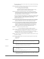
Example 1.
(Cr).
S.S.
123456789 46518519 46517519 56518 46517518 4651751C 4651851B 56517
4651B51C
10 20 21 30 31 32 40 41 42 43 50 51 52 53 54
Notes
The configurations and (optional) orbital (re-) definition are as in SUPERSTRUCTURE (because
of S.S. tag). However, nothing is read from line 2 in columns 1-10, while columns 73-80 should be
left blank. See the Appendix for an explanation of how to specify new, or read existing,
configuration lists.
Namelists:
SALGEB:
RUN = ' ', default. Allows calculation of energies (LS or IC), radiative rates (if RAD
is set) and autoionization rates (if continuum present - see optional input
below).
= 'PI', will calculate (non-resonant) photo-ionization as well if continuum
orbitals are present.
= 'DR','RR','RE','DI','REDA' or 'YES'. All expect one or more Rydberg orbitals to
be defined (via the orbital definition list - see optional input below) and will
read the optional namelist DRR to define the nl values of the Rydberg series
to be run over. 'DR' calculates energies, radiative and autoionization rates.
'RR' calculates non-resonant radiative recombination in addition. In both
these cases, if no radiation is specified, E1 will be switched on.
'RE','DI','REDA' are all equivalent and differ from 'DR' only via 'NO'
radiation being a valid option.
RAD = 'E1' or 'YES' for electric dipole radiation. (Default for RUN='DR' etc.)
= 'NO' for no radiative data. (Default for RUN=' ')
= 'E2' or 'M1' for electric quadrupole and magnetic dipole radiative transitions,
in addition to electric dipole.
CUP = 'LS' for LS-coupling. (Default)
= 'IC' for intermediate coupling.
= 'ICR' for IC using semi-relativistic wavefunctions.
KORB1 and KORB2 or KCOR1 and KCOR2 denote closed shells (use one or the
other) e.g. KORB1=1 KORB2=3 denotes a Ne-like core (assuming standard
order).
MSTART=0 (default) does nothing.
=1 writes the angular algebra to file RESTART
=4 reads the angular algebra from RESTART. This is useful for iso-electronic
runs in cases when the angular algebra takes a significant time to compute.
(=2,3 restarts an incomplete calculation of RESTART.)
KUTSS controls valence-valence two-body fine-structure interactions.
=-1 None. (Default)
=-9 All.
|KUTSS| .gt. 1 includes the interactions for the first |KUTSS| configurations, KUTSS
positive neglects the interaction between distinct configurations.
KUTSO controls the evaluation of the generalized spin-orbit parameter.
= 0 All.
< 0; include interactions between the first -KUTSO configurations and within a
configuration for the remainder. (Default=-1)
ADAS User manual
Chap8-01
17 March 2003
> 0; include interactions within a configuration for the first KUTSO
configurations and neglect all for the remainder.
KUTOO controls the evaluation of the two-body non-fine-structure interactions viz.
contact spin-spin, two-body Darwin and orbit-orbit (only available in IC).
= 0 or -1 neglected. (Default)
else all included.
NAST= The number of distinct SLp terms (listed following if .gt. 0 as 2S+1 L p)
generated from the configuration list, can be used with care in IC. If .eq. 0 all
possible terms are generated (default).
KCUT= 0 all configurations are treated as spectroscopic (default).
> 0 configuration numbers greater than KCUT are treated as correlation, terms
are only generated from them if they also exist in the spectroscopic list.
Correlation terms are ignored when forming the energy functional during
optimization and no transition probabilities (autoionization or radiative) are
calculated for them.
If the first four characters of line 1 are A.S. then two new variables must be
defined:
MXVORB is the number of distinct valence orbitals required to describe the
configurations.
MXCONF is the number of configurations.
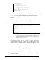
Example 2.
(Cr again).
A.S. The rest of the first line can be used as a header e.g. Cr 7S-7P
&SALGEB RUN=' ' RAD='YES' CUP='LS' MXVORB=7 MXCONF=8
KORB1=1 KORB2=5 NAST=2 KUTSS=-1 KUTSO=-1 KUTOO=-1 &END
3 2 4 0 4 1 4 2 4 3 5 0 5 1
4 0 1 1 0 0 0
4 1 0 1 0 0 0
5 0 1 0 0 0 0
4 1 1 0 0 0 0
4 1 0 0 0 0 1
4 0 1 0 0 1 0
5 1 0 0 0 0 0
4 0 0 0 0 1 1
7 0 0
7 1 1
Notes
1. The alternative (new) way of inputting configurations.
2. Using the configurations of the first example would have been time consuming without the use
of NAST as they contain hundreds of terms.
3. The NAMELIST specification must start in column 2 or greater (at least with many
FORTRAN77 compilers).
SMINIM:
NZION = Nuclear charge. This must be set.
.gt. 0 radial functions are calculated in TFDA potential.
.lt. 0 radial functions are calculated in Hartree potential evaluated with SlaterType-Orbitals. (Preferred)
By default, nl-dependent operation is assumed and the orbitals are Schmidt
orthogonalised. Even if the orbitals happen to be orthogonal there is little
overhead to the nl-dependent operation and it is not worth the hassle
switching it off.
.eq. 0 stops the code after computation of the angular algebra. Useful for restart.
INCLUD .eq. 0 no variational procedure. (Default)
.gt. 0 include the lowest INCLUD terms in the energy-sum to be minimised.
.lt. 0 include -INCLUD terms in energy sum, the T-index labels and weighting
factors follow next (before the lambdas, see below).
ADAS User manual
Chap8-01
17 March 2003
Note: the T-index is required, not the I-index. This is output on the term energy
list from a trial run.
NLAM is the number of (lambda) scaling parameters. Both TFDA and STO Hartree
potentials contain a radial scaling parameter.
= 0 all lambda's equal unity. (Default)
If NLAM is less than the number of orbitals then the last scaling
parameter read will be used for the remaining orbitals.
NVAR is the number of variational parameters. This decoupling of NVAR and
NLAM greatly simplifies the variational operation. NVAR orbital numbers
will be read and their scaling parameters varied. (The variation only takes
place when INCLUD is set non-zero.) Default=0.
Note: The scaling/variational parameters are normally positive numbers around
1. This gives a "physical" orbital. Pseudo-orbitals are generated with negative
lambdas. The default is a screened hydrogenic potential of charge
|lambda*NZION|. However, if
ORTHOG='LPS' then Laguerre pseudo-states are generated for that nl. The lambda is
then the scaling parameter associated with the Laguerre orbital, with the Z
dependence factored out so that |1.0| is usual. Only specify if needed.
MCFMX: Case of STO Hartree/X potentials. MCFMX configuration numbers are
read, one for each orbital. The Hartree potential, for each orbital, uses the
occupation numbers from the specified configuration. If the number of
orbitals is .gt. MCFMX the last configuration is used for the remaining
orbitals. Default=0, and an average of all configurations is used.
MEXPOT = 0 (default) the STO potential is Hartree.
= 1 a local exchange term is added to the Hartree potential.
PRINT='FORM' (default) gives detailed formatted output (to file olg) for a structure
run. Energy/Rate files for DR/RE run are formatted (ols, oic, opls, opic).
='UNFORM', limited writes to file olg and the Energy/Rate files for DR/RE are
unformatted (olsu, oicu) but opls & opic are still formatted.
RADOUT='YES' produces a radial file (radout) suitable for R-matrix STG1 S.S. style.
='NO' doesn't. (Default)
RAD='BF' only produces radiative rates between autoionizing and true bound states
(useful for DR).
=' ' Default, all.
Example 3.
(Cr still).
&SMINIM NZION=24 INCLUD=-1 NLAM=12 NVAR=2 PRINT='FORM' RADOUT='NO'
&END
6 1.0
1.4361 1.1326 1.0754 1.0816 1.0636 1.0878 0.9223 0.9446 -0.4324 0.0000
1.0000 1.0000
11 12
Note:
Example 4.
The 5s and 5p orbitals (11 and 12) are being optimised on term number 6 of the term table, which
wasn't the lowest in energy hence INCLUD=-1. Note also that the 4d is a scaled hydrogenic orbital
and the 4f orbital is not being used, its lambda value is irrelevant.
(Si11+).
S.S.
123456789 11522 11512513 11523
21512 21513
21514 21515 21516
10 20 21 30 31 32
&SALGEB RAD='E1' CUP='IC' KUTSS=-1 KUTSO=-1 KUTOO=-1 &END
&SMINIM NZION=-14 PRINT='FORM' MCFMX=6 &END
6 2 2 6 7 8
Note
ADAS User manual
The orbital must appear in the configuration specified for its generation. Thus, if any other
configuration besides 6 had been specified for orbital 4 (the 3s) an error would have resulted. No
scaling parameters were specified so they would be taken to be unity, which is a much better
approximation than for TFDA.
Chap8-01
17 March 2003
Supplementary input (required for subsequent processing by ADAS702 and ADAS703):
The orbital (re-) definition list is used to "tag" orbitals for special attention if their principal
quantum numbers are as follows:
n=90-99: A continuum orbital. If continuum orbitals are present then SR.RADCON is
entered for their generation and a namelist SRADCON is read to control it.
SRADCON:
MENG is the number of interpolation energies. MENG energies (in Rydbergs) follow
and the continuum orbitals are calculated at those energies.
.lt. 0, only the range need be specified and the -MENG interpolation energies
will be chosen internally.
NREL, there is no interpolation of the bound-continuum relativistic integrals. They
are calculated at a single energy. The NREL'th interpolation energy is used.
Defaults to (MENG+1)/2 if not specified.
Example 5.
(LMM transitions in Si11+).
S.S. A short TITLE (8 chars.) may be set in SALGEB, or a longer one here.
123456789 24 14515 14516 25 15516 26
12518 12519 1251A 1251B 1251C
13518 13519 1351A 1351B 1351C
12514 12515 12516
13514 13515 13516
10 20 21 30 31 32
900901902903904
&SALGEB RUN=' ' RAD='E1' CUP='IC' KCOR1=1 KCOR2=1 TITLE='2-3,3' &END
&SMINIM NZION=-14 PRINT='UNFORM' MCFMX=8 &END
17 17 20 1 2 3 0 7
&SRADCON MENG=-10 &END
2.0000
15.0000
Note: Ten interpolation energies are used, between 2.0 and 15.0 Rydbergs. All of the continuum orbitals will
be generated using the Hartree potential with occupation numbers given by configuration 7. The
requirement that the orbital belong to the configuration is relaxed for continuum orbitals, the
configuration merely has to a contain a continuum orbital.
For RUN=' ', as here, the continuum orbital angular momenta are those specified on
the orbital definition line. Thus we have ks, kp, kd, kf and kg continua.
For RUN.ne.' ' the continuum angular momenta are "matched" to that of the valence
orbital (defined by n=80-89, see next section) but those with n=99 are
NEVER redefined. This is important for inner-shell transitions which may
have an autoionization pathway that is independent of the Rydberg orbital.
Note: it makes no sense (and could cause problems here) to define two
continuum orbitals n=90-98 with the same angular momentum.
n=80-89: A valence/Rydberg orbital that will be redefined in DR/RE operation. If RUN.ne.'
' the namelist DRR is read to define the nl-values that AUTOSTRUCTURE will loop-over for
these orbitals.
DRR:
NMIN, NMAX: Loop the valence orbital over n=NMIN to NMAX incrementing n by
1.
JND = 0, default.
.gt. 0, then JND additional n-values are read following the namelist. AS inserts
an additional n-value between each input value to aid interpolation and
numerical integration over n in the post-processing routines.
NRAD =50, default. In DR runs the radiation from high-n is negligible and the effect
of the Rydberg orbital on the core is small. So, for n.gt.NRAD no new
radiative rates are calculated. The default value is sufficient for most cases.
LMIN, LMAX: Loop the valence orbital over l=LMIN to LMAX incrementing l by 1.
If no valid LMIN & LMAX are set then the loop over n is done using the
ADAS User manual
Chap8-01
17 March 2003
angular momenta specified in the orbital definition. This enables l-mixing
along a Rydberg series to be investigated.
LCON is the number of continuum orbitals used with n=90-98. This is not used if
there is no loop over valence l. As noted above, the continuum orbitals (n=9098, only) must have their angular momenta kept synchronised with that of
the valence orbital. Let lc denoted the continuum angular momenta and lv the
valence angular momentum. Then the internal assignement is lc=lv-(LCON1)/2, lv-(LCON-1)/2 +1, ...... , lv+LCON/2. Generally, LCON should be set
(and the appropriate orbitals and configurations defined) to 2*LAMAX+1
where LAMAX is the largest target multipole transition required. Thus,
LCON=3 for dipole, and =5 for quadrupole core transitions as well.
Example 6.
(Si11+ DR via 2s-2p core transition).
S.S.
123456789 12515 13515
12517 12518 12519
13517 13518 13519
22 12513 23
10 20 21
801
900901902
&SALGEB RUN='DR' RAD='E1' CUP='IC' TITLE='2-2,n' KCOR1=1 KCOR2=1 &END
&DRR NMIN=8 NMAX=15 JND=14 LMIN=0 LMAX=13 LCON=3 &END
16
20
25
35
45
55
70 100 140 200 300 450 700 999
&SMINIM NZION=-14 PRINT='UNFORM' MCFMX=7 &END
3 1 2 0 1 0 3
&SRADCON MENG=-7 &END
0.00 2.50
Notes
1. The angular momenta of the valence and continuum orbitals in the orbital redefinition list is
arbitrary, although in the case of the continuum they should be distinct. The choice of n=80 is
arbitrary, any value between 80 and 89 would suffice. Similarly, for the continuum any value
between 90 and 98 would suffice (but NOT 99).
2. Only outer electron radiation into the core is specified. Outer electron radiation into higher states
will be added-in (hydrogenically) during post-processing.
Example 7.
(Si11+ DR via an inner-shell transition, 1-3).
S.S.
123456789 11512514517 11512515517 11512516517
11513514517 11513515517 11513516517
21512518 21512519 2151251A 2151251B 2151251C
21513518 21513519 2151351A 2151351B 2151351C
11522518 11522519 1152251A 1152251B 1152251C
11512513518 11512513519 1151251351A 1151251351B 1151251351C
11523518 11523519 1152351A 1152351B 1152351C
2151751D 2151751E 2151751F
2151751G
21514518 21515518 21516518
21514519 21515519 21516519
2151451A 2151551A 2151651A
2151451B 2151551B 2151651B
2151451C 2151551C 2151651C
21513514 21513515 21513516 21513517
21512514 21512515 21512516 21512517
10 20 21 30 31 32802900901902903904990991992 X
993
&SALGEB RUN='DR' RAD='E1' CUP='IC' TITLE='1-3,n'
KORB1=0 KORB2=0 &END
&DRR NMIN=4 NMAX=10 JND=0 LMIN=0 LMAX=2 LCON=5 &END
&SMINIM NZION=-14 PRINT='UNFORM' MCFMX=8
&END
7 7 12 1 2 3 1 7
&SRADCON MENG=-15 &END
0.0000 200.0000
Notes
1. The D, E, F and G continuum orbital angular momenta do not get redefined.
2. We allow for quadrupole transitions (LCON=5).
3. It is safest to define only those continuum orbitals that are used in the configuration list.
4. The target + continuum configurations 1s22s, 1s22p, 1s2s2p, 1s2s2, 1s2p2, 1s23s, 1s23p, 1s23d
+e- should have the same continuum expansion attached to them. If the 1s2s2 had orbitals
8,9,A,B,C attached but the 1s2p2 8,A,C only, say, then there would be no mixing between the 1s2s2
and 1s2p2 1S terms for the 1s2s2 9 and B configurations. This will cause the post processor some
problems.
5. The orbital definition list was extended to a second line using a non-blank character in column
63. The orbital definition list is formatted (T16,15(I2,A1)). Hence the continuation mark is two
spaces past the last (15th) orbital.
Example 8.
(Si11+ LMn with l-mixing within the complex).
S.S.
ADAS User manual
Chap8-01
17 March 2003
123456789 14517
14518
14519
1451A
1251B
1351B
12514
13514
15517 16517
15518 16518
15519 16519
1551A 1651A
1251C 1251D 1251E 1251F 1251G
1351C 1351D 1351E 1351F 1351G
12515 12516 12517 12518 12519 1251A
13515 13516 13517 13518 13519 1351A
10 20 21 30 31 32800801802803900901902903904 X
905
&SALGEB RUN='DR' RAD='E1' CUP='IC' KCOR1=1 KCOR2=1 TITLE='2-3,n' &END
&DRR NMIN=4 NMAX=9 JND=0 LMIN=0 LMAX=-5 &END
&SMINIM NZION=14 PRINT='UNFORM' MCFMX=0 &END
&SRADCON MENG=-15 &END
00.0000
25.0000
Note
Only l-mixing for 0,1,2,3 is investigated here. Also we cannot start with n .le. 3 the maximum lmixing investigated. Thus the lowest few n must be run separately. LCON is not required.
n=70-79: An orbital to be replaced in SR.RADWIN. If there exists an orbital tagged for
replacement SR.RADWIN is entered and a namelist is read.
SRADWIN
KEY=-9, default.
If the input file (radwin) is in Opacity Project format (approx. the old IMPACT
format) nothing need be entered here. See code for details of alternative
formats i.e. different KEY values.
Example 9.
(Cr yet again).
A.S.
Cr MCHF
&SALGEB RUN=' ' RAD='E1' CUP='LS' MXVORB=7 MXCONF=8
KCOR1=1 KCOR2=-5 NAST=2 &END
71 0 72 0 72 1 73 0 73 1 73 2 74 0 74 1 74 2 74 3 75 0 75 1
4 0 1 1 0 0 0
4 1 0 1 0 0 0
5 0 1 0 0 0 0
4 1 1 0 0 0 0
4 1 0 0 0 0 1
4 0 1 0 0 1 0
5 1 0 0 0 0 0
4 0 0 0 0 1 1
5 0 0
5 1 1
&SMINIM NZION=24 PRINT='FORM' &END
&SRADWIN &END
Notes
1. The use of negative KCOR2 to read ALL nl definitions (as we must if we want to replace the
core orbitals as well as the valence) but valence occupation numbers only for the configurations.
2. All of the orbitals are tagged for replacement so SMINIM requires little input. Although the use
of 71 0 72 0 is suggestive of 1s and 2s replacement (and helpful) it should be noted that the 1st
orbital (71 0) will be replaced by the first s-orbital in the file radwin. We could have written 72 0
71 0 and the same result would be obtained, if somewhat confusing - the 1s orbital (assuming it was
infront of the 2s on radwin) would be in 72 0.
Appendix: Eissner configurations are defined by occupation numbers and orbital numbers.
Each occupation/orbital-number pair is separated from the next by a '5'. Each configuration
is separated from the next by a blank. They do not have to fill the line, but a new line of
configurations must start with column 11. Unless redefined after the configuration list (see
example 1, where the "redefinition" is actually a specification of the default) the orbital
numbers (actually alphanumerics) are associated with nl pairs as follows:
0
=
l
n=1
n=2
n=3
n=4
n=5
1
2
4
7
B
.
.
l
3
5
8
C
l
9
3
=
l
A
E
.
2
=
6
D
.
1
=
4
=
l
F
.
.
etc.
The horizontals of the triangle of numbers are of constant n and the upward (positive
gradient) diagonals are of constant l. After 9 the numbers become UPPER CASE letters and
eventually lower case letters (you shouldn't need them!). E.G. the configuration 2s 2p2 3d is
rendered as 12523516 .
ADAS User manual
Chap8-01
17 March 2003
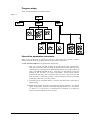
Program steps:
These are summarised in the schematic below.
Figure 7.1
0$,1
$/*(%
=(52
0,1,0
$/*(%
$/*(%
'HWHUPLQH 1RQUHODWLYLVWLF
DQJXODU
DOO WHUPV
DOJHEUD
RI
DQG
FRQILJXUDWLRQV VWUXFWXUH
UDGLDWLYH
DOJHEUD
$/*(%
5HODWLYLVWLF
DOJHEUD
UHFRXSOLQJ
5$',$/
%RXQG
RUELWDO
JHQHUDWLRQ
5$'&21
&RQWLQXXP
RUELWDO
JHQHUDWLRQ
5$':,1
)HHG LQ
DQ\
H[WHUQDO
RUELWDOV
',$*21
'HWHUPLQH
QRQUHODWLY
VWUXFWXUH
HOHYHOV
HYHFWRUV
UDGLDWLYH DXWRLRQ UDWHV
',$*)6
'HWHUPLQH
UHODWLYLVWLF
VWUXFWXUH
HOHYHOV
HYHFWRUV
UDGLDWLYH DXWRLRQ UDWHV
Interactive parameter comments:
Move to the sub-directory in which you wish text output from this program to appear.
Initiate ADAS701 from the program selection menus in the usual manner.
The file selection window has the appearance shown below
1. Data root a) shows the full pathway to the appropriate data sub-directories.
Click the Central Data button to insert the default central ADAS pathway to the
correct data type. The appropriate ADAS data format for input to this program is
adf27 (‘AUTOSTRUCTURE drivers’). Click the User Data button to insert the
pathway to your own data. User Data is the default. Central ADAS contains
samples from which the user can build his/her own driver. Note that your data
must be held in a similar file structure to central ADAS, but with your identifier
replacing the first adas, to use this facility.
2. The Data root can be edited directly. Click the Edit Path Name button first to
permit editing.
Available sub-directories are shown in the large file display window b). Scroll bars
appear if the number of entries exceed the file display window size. The practice
in ADAS is to store drivers in sub-directories according to iso-electronic
sequence of the recombining ion (eg. /belike).
ADAS User manual
Chap8-01
17 March 2003
ADAS701 INPUT
Data Root
/disk2/adas/adas/adf27/
Edit Path Name
User data
Central data
a)
helike/ne8ic_sat.dat
c)
QHLFBVDWGDW
'DWD )LOH
b)
Cancel
Browse Comments
Done
3. Click on a name to select it. The selected name appears in the smaller selection
window c) above the file display window. Then its sub-directories in turn are
displayed in the file display window. The individual data files all have the
termination .dat. The purpose of the driver data set is indicated by the pattern of
the file name as
/<ion><coupling>{<prt-trans>}{-<n-shell>}{_<task>}.dat
where
<ion> denotes the recombining ion (eg. ‘o4’ for O+4)
<coupling> denotes the coupling scheme (‘ls’ for LS-coupling,
‘ic’
for intermediate coupling)
<prt-trans> denotes the parent n-n’ shell transition (eg. ‘23’).
This
name portion does not appear for task ‘sat’ below ‘
<n-shell> denotes the outer n-shells treated, which may be a single
shell (as eg. ’3’) or all n-shells (as eg. ‘n’)
This name portion does not appear for tasks ‘.str’
and ‘.sat’ below.
<task> denotes the objective (‘str’ for the baseline structure
calculation, ‘sat’ for satellite line data preparation) If
the field is blank then the main Auger and radiative rate
calculations for dielectronic rates take place.
Thus ‘o4ls23_str.dat’ is a driver for the n=2-3 parent transition related LS-coupled
term structure calculation used to establish the resonance positions. ‘o4ls233.dat’ and ‘o4ls23-n.dat’ are for the dielectronic rate calculations with only the
n=3 outer electron present and for all outer n-shells respectively. ‘o4ls_sat.dat’
is for the preparation of Auger/radiative data for satellite line modelling.
4. Once a data file is selected, the set of buttons at the bottom of the main window
become active.
5. Clicking on the Browse Comments button displays any information stored with
the selected data file. It is important to use this facility to find out what is
broadly available in the data set. The possibility of browsing the comments
appears in the subsequent main window also.
6. Clicking the Done button moves you forward to the next window. Clicking the
Cancel button takes you back to the previous window
There is no processing options window
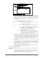
The output options window appearance is shown below. Note that there is no graphical output in
this case
7. The full pathway to the driver data set to be used is shown for information at the
top of the window and at a) the Browse comments button is available. A title for
the run may also be entered in the text widget just below.
ADAS User manual
Chap8-01
17 March 2003
$'$6 287387 237,216
'DWD )LOH 1DPH GLVNDGDVDGDVDGIKHOLNHQHLFBVDWGDW
%URZVH FRPPHQWV
7LWOH IRU 5XQ
GHPRQVWUDWLRQ
D
'LUHFWRU\ IRU $8726758&785( ILOH RXWSXW
KRPHPRJDGDVDXWRV
E
6HOHFW W\SH RI UXQ 6WUXFWXUH
6DWHOOLWH
5DWHV
:ULWH WKH IROORZLQJ RXWSXW ILOHV UDGZLQ
ROJ
ROJ
UDGZLQ
ROV
ROV
UDGRXW
UDGRXW
7(506
RLF
RLF
7(506
ROVX
ROVX
/(9(/6 /(9(/6
RLFX
RLFX
RSOV
RSOV
5(67$57
5(67$57
RSLF
RSLF
7H[W RXWSXW
)LOH 1DPH &DQFHO
5HSODFH
F
G
'HIDXOW ILOH QDPH
SDSHUW[W
5XQ 1RZ
H
5XQ LQ %DWFK
I
8. The sub-window at b) allows selection of which output files from ADAS701 are
to be kept and the names to be assigned to them. Up to twelve output files are
available in principle. The default file names are shown and their contents are
as follow:
olg
detailed (diagnostic) output.
ols
energies & radiative and autoionisation rates between terms
(formatted).
oic
energies & radiative and autoionisation rates between levels
(formatted).
olsu energies & radiative and autoionisation rates between terms (unformatted).
oicu energies & radiative and autoionisation rates between levels (unformatted).
RESTART
restart file
.
radwin
input file of externally prepared radial orbitals.
radout
output file of internally calculated radial orbitals.
TERMS
term labelling.
LEVELS
level labelling.
opls LS-coupling photo-ionisation cross-sections.
opic intermediate coupling photo-ionisation cross-sections.
9. The pathway to the directory where you wish to place the saved files in entered
at b). The default is to the sub-directory ‘/…/<user>/adas/autos’ . This is a
sub-directory like the usual /pass sub-directory but is dedicated to ADAS7 series.
The output may be quite substantial and exceed small workstation capacities.
The text widget is editable, so an alternative path may be substituted for the
default.
10. At c) , the button for the type of run is clicked. This matches the driver data set
names ‘str’, ‘sat’ and ‘’ described above. According to your choice, various of
the temporary output files are selected for saving. The text widgets are editable
and you can replace default names by names of your choice. Warnings may be
issued below the file names if a file already exists and will be over-written. This
is simply a warning for the user to take action before proceeding if desired.
There is no further protection. Note that the same standard names are always
used by default and so the user must rename if he wishes to keep data.
ADAS User manual
Chap8-01
17 March 2003
Deselected output files will be eliminated in a clean-up after the code has
completed. For dielectronic rate production, it is usual to do the calculation in a
number of stages (cf. the drivers o4ls23-3.dat and o4ls23-n.dat). The Auger &
radiative rate coefficient files ,‘ols’ - for LS coupling or ‘oic’ for intermediate
coupling, should be renamed for each stage successively as ‘o1’, ‘o2’, etc. This
is the responsibility of the user. Note that both formatted (eg. ‘oic’) and
unformatted (eg. ‘oicu’) forms of the files can be produced. For large runs it is
much more economical to use the unformatted forms and they are similarly
renamed (eg. ‘o1u’).
11. At d) the Text Output button activates writing to a text output file. The file
name may be entered in the editable File name box when Text Output is on. The
default file name ‘paper.txt’ may be set by pressing the button Default file name.
A ‘pop-up’ window issues a warning if the file already exists and the Replace
button has not been activated.
12. At the base of the graph window, buttons are available for selection of
foreground execution (Run Now), or batch submission (Run in Batch). Click
Cancel to return to the input driver selection window without execution.
Notes:
1. The code can use substantial computer resources in complex ion cases. It has been
compiled with dimensions set for medium-sized cases compatible with average
workstation capacity. Abnormal termination of the code may result from exceeding these
dimensions. Failure diagnostic information and recommendations are given at the end of
the olg file. Please notify ADAS support if re-dimensioning is required.
2. The code requires IDL version 4 or later. If this is not available on your machine, ADAS
support (University of Strathclyde) has some capacity for executing tasks on your behalf.
ADAS User manual
Chap8-01
17 March 2003