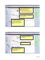
1
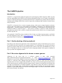
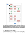
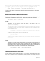
X-MATE user manual Version 1.0 September 2010 Contact: [email protected] Institute for Molecular Bioscience The University of Queensland St Lucia, QLD, 4072 Page 1 of 41 License: This software is copyright 2010 by the Queensland Centre for Medical Genomics. All rights reserved. This License is limited to, and you may use the Software solely for, your own internal and non-commercial use for academic and research purposes. Without limiting the foregoing, you may not use the Software as part of, or in any way in connection with the production, marketing, sale or support of any commercial product or service or for any governmental purposes. For commercial or governmental use, please contact [email protected]. In any work or product derived from the use of this Software, proper attribution of the authors as the source of the software or data must be made. The following URL should be cited: http://grimmond.imb.uq.edu.au/X-MATE/ This package is distributed in the hope that it will be useful, but WITHOUT ANY WARRANTY; without even the implied warranty of MERCHANTABILITY or FITNESS FOR A PARTICULAR PURPOSE. Applied Biosystems Software components distributed with this package carry their own license agreements, located at the following URLs: MaToGff: http://solidsoftwaretools.com/gf/project/matogff/ GffToSam: http://solidsoftwaretools.com/gf/project/sam/ Mapreads: http://solidsoftwaretools.com/gf/project/mapreads/ We thank and acknowledge the contributions of the developers of the above packages, as well as Applied Biosystems for making the packages available with the X-MATE system. Page 2 of 41 X-MATE user manual ...........................................................................................................................1 License: ................................................................................................................................................................................2 List of Figures.........................................................................................................................................4 The X-MATE pipeline ...........................................................................................................................5 Introduction.......................................................................................................................................................................5 Part 1: Quality checking of the tag (optional) .....................................................................................................5 Part 2: Recursive alignment to the human or mouse genome.....................................................................5 Part 3: Multi-‐mapping tag rescue (optional).......................................................................................................6 Part 4: Creation of visualization and SAM files ..................................................................................................7 Availability .........................................................................................................................................................................7 Requirements....................................................................................................................................................................7 Installation instructions (X-‐MATE) .........................................................................................................................8 Installation Instructions (SamConverter) ............................................................................................................9 Testing and Configuration .............................................................................................................. 10 Testing X-‐MATE (mapreads)................................................................................................................................... 10 Testing X-‐MATE (ISAS Colors)................................................................................................................................ 11 Testing X-‐MATE (ISAS Bases) ................................................................................................................................. 13 Configuration file.......................................................................................................................................................... 13 Configuration options................................................................................................................................................. 14 Selecting appropriate parameters ........................................................................................................................ 19 How to map to the genome and junctions simultaneously ........................................................................ 22 How to use X-‐MATE to perform non-‐recursive mapping ........................................................................... 22 X-MATE Functionality and Output Files ..................................................................................... 22 Log File.............................................................................................................................................................................. 22 Checking the finished run......................................................................................................................................... 24 Description of output files........................................................................................................................................ 25 Re-‐entering the X-‐MATE pipeline ......................................................................................................................... 26 Modifying the pipeline to work with other queues ....................................................................................... 27 Optimizing performance on your cluster .......................................................................................................... 27 Creating SAM files .............................................................................................................................. 28 Scripts .................................................................................................................................................... 29 Master script: X-‐MATE.pl .......................................................................................................................................... 29 Modules ............................................................................................................................................................................ 30 Post-X-MATE scripts ......................................................................................................................... 30 Filtering wiggle plots .................................................................................................................................................. 30 Assessing the specificity of mapping ................................................................................................................... 30 Checking the mapping statistics ............................................................................................................................ 31 Cleaning up after a mapping run ........................................................................................................................... 31 Writing SAM Converter configuration files....................................................................................................... 31 Assigning tags or coverage counts to gene models ....................................................................................... 32 Junction libraries ............................................................................................................................... 39 Description of the available junction libraries ................................................................................................ 39 How to create your own junction libraries ....................................................................................................... 40 How to make ISAS junction libraries ................................................................................................................... 40 A note on ISAS performance........................................................................................................... 41 Page 3 of 41 Supplimentary figure 4 .................................................................................................................... 41 List of Figures Figure 1. The X-MATE recursive mapping pipeline. The pipeline consists of 4 major components. (1) The optional tag quality module filters tags based on the quality values for each basecall. (2) The alignment module attempts to align tags first to the genome, and then to a library of known exon-junction sequences (if mapping RNA-Seq data). If a tag fails to align, then the tag is truncated, and the process is repeated. (3) The optional tag rescue module uses information derived from both single-mapping and multi-mapping tags to uniquely place multi-mapping tags. (4) Finally, UCSC genome browser compatible wiggle plots and BED files are generated. A final optional step creates SAM files. ........................ 6 Figure 2. Effect of length and mismatches on the specificity of mapping tags. For each length and mismatch combination, the proportion of tags that map uniquely within the human genome is indicated by the green line. The blue line indicates the proportion of tags that map to exons, and shows a steep decline at 25.3 and 23.5, indicating a drop in specificity at this length. The total number of tags mapping at a given length and ................................... 19 Figure 3. How alternate mapping strategies affect the yield of mappable tags and the computational run time. In all graphs, red lines represent Strategy 1 (2nt interations, 50nt30nt), blue lines represent Strategy 2 (5nt interations, 50nt-25nt), and green lines represent Strategy 3 (10nt iterations, 50nt-30nt). In all scenarios, 5 mismatches were allowed for tag lengths ranging from 50nt to 40nt, 3 mismatches were allowed for tag lengths ranging from 39nt to 30nt, and 1 mismatch was allowed for tag lengths ranging from 29nt to 25nt. Scenario One is a fragment library with a mode insert size of 54nt; Scenario Two is the same library with the insert size shifted to 39nt. Together, these graphs show that there is more benefit for a recursive strategy when the library insert size is smaller than ideal....... 21 Figure 4. Quality profile for a recursive mapping run on approximately 10 000 000 base space reads (Illumina GAII, SRA accession ERR000099, mapped using ISAS). Each line represents a mapping run for a single recursive iteration (N.M, N = read length, M = mismatches). Although the tags are mapped at progressively shorter lengths, the quality values are reported for the complete (un-truncated) length of every tag. Tags that map at shorter lengths contain on average lower quality bases towards their 5’ end. ..................... 41 Page 4 of 41 The X-MATE pipeline Introduction X-MATE is a computational pipeline designed for the rapid mapping of DNA fragment or RNA-seq data from the Applied Biosystems SOLiD system. Built and production tested to run on modest computational resources, X-MATE generates tag count and genome-browser visualization of genomic and exon-junction matching results (Wiggle, BED), and a variety of output files (including SAM) suitable for further tertiary analysis software. X-MATE is a framework for a recursive mapping strategy, where tags are mapped against a reference genome, and if not mapped (at a certain number of mismatches), truncated by a user-defined length and mapped again. Recursive mapping is optional, but recommended. A diagrammatic representation of the X-MATE workflow is shown in Figure 1. The recursive workflow is similar for both stranded and unstranded (eg genomic) data, with the exception that optional junction libraries may be mapped against for RNA-Seq data sets. Also optionally, X-MATE has been extended to allow for the use of other mapping engines, specifically the rapid alignment system, ISAS (www.imagenix.com). The following sections describe each of the parts of the X-MATE workflow as shown in Figure 1. Part 1: Quality checking of the tag (optional) Depending on the downstream applications of the matched data the quality of individual tags may need to be assessed before their inclusion in the mapping pipeline. To accommodate this, we have provided an optional tag quality module that assesses the tags by the number of basecalls with PHRED scores of less than 10. Tags that pass the QC are fed into the recursive alignment module. If this option is disabled, all tags are passed to the alignment module. Part 2: Recursive alignment to the human or mouse genome Alignment of the short tags to a reference genome is done using mapreads (http://solidsoftwaretools.com/gf/project/mapreads/), or ISAS (http://www.imagenix.com). Both algorithms are specifically designed for the rapid mapping of data from the Applied Biosystems SOLiD system (ie. color-space data), although base-space (fastq file format for ISAS and fasta format for mapreads) data sets can be mapped using X-MATE also. Tags are first matched against all chromosomes of the reference genome, and then optionally against a library of known exon-junctions for RNAseq data sets (hg18, hg19 and mm9 are currently supported). Tags that fail to map to the genome or junctions are chopped to user-defined lengths, and the genomic mapping is restarted. In this way, tags that have adaptor sequence, or poor quality ends are recovered at their longest length. The number of mismatches between the reference and tag is user defined. Page 5 of 41 Figure 1. The X-MATE recursive mapping pipeline. The pipeline consists of 4 major components. (1) The optional tag quality module filters tags based on the quality values for each basecall. (2) The alignment module attempts to align tags first to the genome, and then to a library of known exon-junction sequences (if mapping RNA-Seq data). If a tag fails to align, then the tag is truncated, and the process is repeated. (3) The optional tag rescue module uses information derived from both single-mapping and multi-mapping tags to uniquely place multi-mapping tags. (4) Finally, UCSC genome browser compatible wiggle plots and BED files are generated. A final optional step creates SAM files. Part 3: Multi-mapping tag rescue (optional) For most downstream applications, tags are only informative if they can be placed uniquely within a genome. Tags that align to multiple places within a genome make up a sizeable proportion of transcriptome derived tags, primarily from the inherent redundancy of the genome, but also from CpG Page 6 of 41 islands and genome wide repeat elements. Strategies to rescue ambiguous sequences have recently been applied to high-throughput sequencing data, and we have refined our previously published algorithm to work efficiently with large data sets. For every multi-mapping tag, the algorithm considers all tags that map near to each of the possible locations of the tag (within a user-specified window) to determine the most likely mapping position of the tag. Where a tag cannot be unambiguously assigned, a fractional weighting to the relevant positions is assigned. In practice, between 40-60% of multi-mapping tags can be assigned a single position with ≥60% likelihood, depending on the relative sequence coverage. The recommended window size for shotgun sequencing is 10 (Cloonan, et al., 2008 Nat Methods 5, 613-619.), though for disparate data types currently available this can vary. For instance, Cap Analysis of Gene Expression (CAGE) tags are rescued using a window of 100nt, a size previously shown to optimize mammalian promoter detection (Carninci, et al., 2006, Nat Genet, 38, 626-635). Part 4: Creation of visualization and SAM files UCSC genome browser compatible wiggle plots for genome mapped data, and BED files for exonjunction mapped data are generated automatically from the collated results. The wiggle plots are strandspecific or un-stranded (depending on experiment requirement), single-nucleotide resolution coverage plots, and directly represent the number of times an individual nucleotide has been seen in the sequencing data. BED files depict hits to junction sequences, and graphically display exon combinatorics. In addition, plots containing only start sites of tags are included to facilitate tag-counting applications. Optionally, SAM (Sequence Alignment Format) files can also be created using the SAMConverter package released with X-MATE (see section Creating SAM files for a description on how to install and use this module). Availability All source code, documentation, and associated files described in this manual are freely available for download from http://grimmond.imb.uq.edu.au/X-MATE/. Requirements This pipeline is written predominantly in perl (with some optional python, Java and C++ thrown in for good measure), and requires that you have version 5.8.8 of perl or later, python 2.4 or later, Java 1.5 or later and a recent version of g++. It is designed to run in a unix environment, with a PBS queue manager (although PBS is not required for SAM conversion and ISAS mapping runs). The scripts can be modified to work with an LSF or SGE manager. It is not recommended to run this pipeline on a system without access to a cluster due to the large computational requirements of mapping to mammalian genomes – however, the scripts could potentially be modified to do this. Required perl modules are (available in CPAN). • Parallel-ForkManager • Path-Class • Object-InsideOut • Devel-StackTrace • Class-Data-Inheritable The alignment section of this pipeline is dependant upon the mapreads tool. This tool and its installation instructions are available from: http://solidsoftwaretools.com/gf/project/mapreads/ (requires registration, which is free). Page 7 of 41 Optionally, in place of mapreads, the alignment software ISAS can be used, and can be licensed from: http://www.imagenix.com/ Finally, you will need a genome against which to map. The program expects one file per chromosome, with the filename format as “[chromosome_name].fa”. Genomes can be downloaded from the UCSC genome browser website at: http://hgdownload.cse.ucsc.edu/downloads.html Installation instructions (X-MATE) The instructions given below in courier font are examples of the commands needed to carry out the installation. X-MATE source is downloaded as a single gzipped tar file. 1. Move the tarball to the destination directory, navigate to your chosen directory and decompress XMATE. mv X-MATE.tar.gz /home/software/ cd /home/software/ tar –xzf X-MATE.tar.gz cd X-MATE/ 2. Create the Makefile by running the command: perl Makefile.PL If you do not have administrator privileges on your system and you would like to install X-MATE in your home directory, you can optionally choose to do this by providing the argument INSTALL_BASE=[full path], eg: perl Makefile.PL INSTALL_BASE=[full path] 3. If the Makefile has been written successfully (there should be a file called Makefile in the source directory), then to run the installation run the following commands: make make install All required perl modules should now be installed in your system’s default perl library location, or in the location specified by INSTALL_BASE above. If the above INSTALL_BASE option is chosen you may also be required to add the path of the installation directory to @INC using the command: export PERL5LIB=${PERL5LIB}:/[full path]/X-MATE/lib/ Where [full path] should be replaced with the path of the X-MATE directory. This command can be added to the ~/.bash_profile or ~/.profile files (depending on the shell) for automatic loading, or it can be added to the default profile for all users. Page 8 of 41 Installation Instructions (SamConverter) The SamConverter utility is a Java application with dependencies on the Applied BioSystem utilities GffToSam and some Java libraries. Specifically the SamConverter utility relies on the following software: • GffToSam o Binary available at http://solidsoftwaretools.com/gf/project/sam/ (requires registration), or, o Source code distributed with X-MATE for compilation if required (see below) Three java archive libraries distributed with X-MATE: • com.apldbio.aga.common.jar (courtesy Life Technologies) • MaToGff.jar (courtesy Life Technologies) • SamConverter.jar (Developed by QCMG) As well as these java library archives (freely available from Apache.org and also distributed with XMATE) • commons-io-1.4.jar (http://commons.apache.org/io/) • commons-lang-2.2.jar (http://commons.apache.org/lang/) • commons-logging-1.1.jar (http://commons.apache.org/logging/) Within the X-MATE distribution is a directory called ‘SamConverter’ it contains a directory ‘jar’ and the jar file samConverter.jar. Also in the SamConverter directory is stored the source code for GffToSam.cpp and a Makefile. To install, follow these instructions: 1. First build the GffToSam utility and install it somewhere onto your $PATH (this may require administration privileges, depending on where you would like to install it. cd SamConverter make cp –p GffToSam /home/software/ 2. Next add the Java archive files to your Java $CLASSPATH, assuming that they reside in the directory [/path/to/jars/], you can enter the following commands: $CLASSPATH=$CLASSPATH:/path/to/jars/commons-io-1.4.jar $CLASSPATH=$CLASSPATH:/path/to/jars/commons-lang-2.2.jar $CLASSPATH=$CLASSPATH:/path/to/jars/commons-logging-1.1.jar $CLASSPATH=$CLASSPATH:/path/to/jars/com.apldbio.aga.common.jar $CLASSPATH=$CLASSPATH:/path/to/jars/MaToGff.jar The SamConverter utility is now ready to be used. Page 9 of 41 Testing and Configuration Testing X-MATE (mapreads) To ensure that your downloads are functioning correctly, please download the testing data (xmate.test.rna.500K.tar.gz) and testing results (test_xmate_rna_colors_mapreads_results.tar.gz) available from: http://grimmond.imb.uq.edu.au/X-MATE/ Please also download the hg19 version of the human genome, available from: http://hgdownload.cse.ucsc.edu/ The testing data includes: • test_xmate_rna_colors_mapreads.conf (the Mapreads test configuration file) • test_xmate_rna_colors_isas.conf (the ISAS test configuration file, see next section). • test_500K_tags_50mers.csfasta (the SOLiD testing data) The testing results folder includes the wiggle plots, start files, collated files and junction BED files that were generated from the testing data on our system: • test_500K_tags_50mers.expect.junc.BED (junction BED file for UCSC genome browser) • test_500K_tags_50mers.unexpect.junc.BED (antisense matches to junctions) • test_500K_tags_50mers.geno.30.3.0.collated (all genomic matches for 30nt tags) • test_500K_tags_50mers.geno.35.3.0.collated (all genomic matches for 35nt tags) • test_500K_tags_50mers.geno.40.5.0.collated (all genomic matches for 40nt tags) • test_500K_tags_50mers.geno.45.5.0.collated (all genomic matches for 45nt tags) • test_500K_tags_50mers.geno.50.5.0.collated (all genomic matches for 50nt tags) • test_500K_tags_50mers.junc.30.3.0.collated (all genomic matches for 30nt tags) • test_500K_tags_50mers.junc.35.3.0.collated (all genomic matches for 35nt tags) • test_500K_tags_50mers.junc.40.5.0.collated (all genomic matches for 40nt tags) • test_500K_tags_50mers.junc.45.5.0.collated (all genomic matches for 45nt tags) • test_500K_tags_50mers.junc.50.5.0.collated (all genomic matches for 50nt tags) • test_500K_tags_50mers.start.negative (wiggle plot of tag start sites for the –ve strand) • test_500K_tags_50mers.wiggle.negative (wiggle plot for the –ve strand) • test_500K_tags_50mers.start.positive (wiggle plot of tag start sites for the +ve strand) • test_500K_tags_50mers.start.negative (wiggle plot for the +ve strand) Edit the configuration file so that it refers to the appropriate directories that you have set up on your system. See the “Configuration Options” section for more details on what each of the parameters does. Run the script, use the following command: nohup perl [path]/XMate.pl –c test_xmate_500K.conf & Page 10 of 41 Where [path] is the full path to X-MATE.pl. eg. nohup perl /data/XMate.pl –c test_xmate_500K.conf & Testing will run X-MATE on the SOLiD test data in approximately 3 hours (using 3 Blades, each with 16GB of RAM and 2 Dual-Core AMD Opteron(tm) Processor 2218 (4 cores), running RedHat Linux 2.6.18-92.1.17.el5 x86_64). Once the run has completed, the results should be compared to those provided in the test_xmate_rna_colours_mapreads_results folder. Additionally, you can check the matching stats using the script provided with X-MATE and the following command: perl [path]/check_matching_stats_XMATE.pl –p [path to results] The output of this script should look like this (assuming you mapped to hg19) Checking directory: output/ Checking genome and junction matches... File: output/test_500K_tags_50mers.geno.30.3.0.collated File: output/test_500K_tags_50mers.geno.35.3.0.collated File: output/test_500K_tags_50mers.geno.40.5.0.collated File: output/test_500K_tags_50mers.geno.45.5.0.collated File: output/test_500K_tags_50mers.geno.50.5.0.collated File: output/test_500K_tags_50mers.junc.30.3.0.collated File: output/test_500K_tags_50mers.junc.35.3.0.collated File: output/test_500K_tags_50mers.junc.40.5.0.collated File: output/test_500K_tags_50mers.junc.45.5.0.collated File: output/test_500K_tags_50mers.junc.50.5.0.collated 50 mers: 107698 45 mers: 26733 40 mers: 28452 35 mers: 8730 30 mers: 26204 Total GB matched: 0.008817635 To clean up the X-MATE output directory, you can run this command: perl [path]/clean_up_XMATE_output_directories –p [pathToResults] This will delete some working files not necessary for standard X-MATE use. More advanced users may want to keep some of these files, so please check if you need them first (see section “Description of output files” for more information). Testing X-MATE (ISAS Colors) If you have ISAS installed, you can also run the following tests to check that X-MATE is working properly with your ISAS installation. Note that first you will need to build the reference sequence indexes for ISAS by following the instructions in the ISAS user manual, as well as the junction libraries for ISAS following the instructions in section “Error! Reference source not found.”. Once these are Page 11 of 41 created, you can use the same test data set as for the mapreads testing (above), but use the configuration file: • test_xmate_rna_colors_isas.conf Edit the configuration values in the [Standard Parameters] section to direct X-MATE to the correct locations for files and output directories. Run the X-Mate.pl script as follows: nohup perl XMate.pl –c test_isas_500K.conf & Once the process has completed, download the ISAS colors testing results (test_xmate_rna_colors_isas_results.tar.gz) available at: http://grimmond.imb.uq.edu.au/X-MATE/ Compare the output with data in the test_xmate_rna_colors_isas_results folder. Note that although this is the same data set as the mapreads tests, and both mapreads and ISAS (at a filter level of 0 – see the ISAS documentation) guarantee to find all alignments within a mismatch range, the results will differ slightly due to the minor differences in mapping strategy. Running the script check_matching_stats_XMATE.pl on this directory will produce the output: Checking directory: test500K/ Checking genome and junction matches... File: test500K/test_500K_tags_50mers.geno.mers25.collated File: test500K/test_500K_tags_50mers.geno.mers35.collated File: test500K/test_500K_tags_50mers.geno.mers40.collated File: test500K/test_500K_tags_50mers.geno.mers45.collated File: test500K/test_500K_tags_50mers.geno.mers50.collated File: test500K/test_500K_tags_50mers.junc.mers25.collated File: test500K/test_500K_tags_50mers.junc.mers35.collated File: test500K/test_500K_tags_50mers.junc.mers40.collated File: test500K/test_500K_tags_50mers.junc.mers45.collated File: test500K/test_500K_tags_50mers.junc.mers50.collated 50 mers: 105548 45 mers: 24632 40 mers: 24800 35 mers: 24322 25 mers: 34300 Total GB matched: 0.00908661 Mapping using ISAS should take about 2 hours on a standard blade. The majority of this time will be parsing and collating the mapped results (ISAS is many times faster than mapreads for mapping but many of the processes in X-MATE are bound by input/ output performance). Page 12 of 41 Testing X-MATE (ISAS Bases) If you have ISAS bases installed, you can use the test X-MATE using the data file xmate.test.dna.500K.tar.gz available at http://grimmond.imb.uq.edu.au/X-MATE/ Once unzipped, this package includes the following files: • • test_xmate_dna_bases_isas.conf (the ISASbases test configuration file) test_dna_500K.fastq (illumina DNA testing data) Modify the configuration file to correctly point X-MATE to the required locations of the ISASbases binary, the output directory and input fastq file. You will also need to create ISASbases indices following the instructions in the ISAS user manual, and point X-MATE to these indices in the configuration file. Once this is complete, launch X-MATE. If the run completes successfully, download the results package (test_xmate_dna_bases_isas_results.tar.gz) and compare your results with those in the results folder. You can also run the script check_matching_stats_XMATE.pl, the output should be equivalent to: Checking directory: . Checking genome and junction matches... File: ./test_isas_dna_500K.geno.mers25.collated File: ./test_isas_dna_500K.geno.mers30.collated File: ./test_isas_dna_500K.geno.mers35.collated File: ./test_isas_dna_500K.geno.mers40.collated File: ./test_isas_dna_500K.geno.mers45.collated 45 mers: 423327 40 mers: 12300 35 mers: 11781 30 mers: 1242 25 mers: 4436 Total GB matched: 0.02010221 Configuration file The configuration file is a text file containing all the required parameters to run X-MATE. Example configuration files are available in src/ folder in the X-MATE distribution. There are eight example configurations, corresponding with the following types of X-MATE runs: Configuration file xmate_dna_colours_mapreads.conf xmate_dna_bases_mapreads.conf xmate_dna_colours_isas.conf Run Type DNA DNA DNA Mapping Engine Mapreads Mapreads ISAS Encoding colorspace basespace colorspace Page 13 of 41 xmate_dna_bases_isas.conf xmate_rna_colours_mapreads.conf xmate_rna_bases_mapreads.conf xmate_rna_colours_isas.conf xmate_rna_bases_isas.conf DNA RNA RNA RNA RNA ISAS Mapreads Mapreads ISAS ISAS basespace colorspace basespace colorspace basespace These configuration files should serve as a starting point for any mapping run. Parameters can be modified in these as required. The following configuration parameters are available in X-MATE: Configuration options [Standard Parameters] exp_name = test_500K_tags_50mers [required] Set the experiment name with this parameter. output_dir = /data/mapping/output [required] Specify the directory where X-MATE will write all output files. raw_csfasta = /data/unmappedData/test.csfasta [required] Specify the location of the raw csfasta file raw_qual=/data/raw/tag20000.qual The full path of the file containing the quality values. expect_strand = + This defines the strandedness of the data. For example, libraries made with the SREK protocol or other direct ligation protocols will have tags that are sequenced in the sense (+) strand relative to the expressed gene. Libraries made with the SQRL protocol will have tags that are sequenced in the antisense (-) relative to the expressed gene. For genomic data, set the strand to ‘0’. raw_tag_length = 35 This parameter defines the longest length of the tags contained in the csfasta file. [genome mapping] – use this section if mapping using Mapreads mask = 11111111111111111111111111111111111 This setting allows you to ignore particular bases in the tag when computing the number of mismatches. 1 = consider this base, 0 = do not consider this base. The length of the mask should equal the length of the longest tags. max_multimatch = 10 Page 14 of 41 Defines the maximum number of positions to be reported for multi-mapping tags. The higher this number, the more disk space is required to store the data, and the slower the program will run. Recommended size for most applications is 10. For interrogating repeat sequences (such as retrotransposable elements) this value may need to be set higher. recursive_maps = = = = = 50.5.0 45.5.0 40.5.0 35.3.0 30.3.0 These parameters define the lengths at which matching will occur recursively, the number of mismatches permissible between the tag and the reference sequence, and whether or not to treat valid adjacent errors as a single mismatch. These are comma separated parameters, with the format of [length].[mismatches].[valid_adjacent]. [length] defines the length of the tag to match at, [mismatches] defines the number of mismatches allowed, and [valid_adjacent] is set to 1 if valid-adjacent errors are to be treated as a single mismatch, or 0 if they are not. In the above example, the recursive mapping will match at lengths 50, 45, 40, 35, and 30. For lengths 50-40, there will be 5 mismatches allowed, whereas for lengths 35 and 30 will allow only 3 mismatches. Valid-adjacent errors are not treated as a single mismatch. For a discussion on selecting optimal parameters for analysis see the section “Selecting appropriate parameters”. genomes =/data/matching/hg19_fasta/chr1.fa =/data/matching/hg19_fasta/chr10.fa =/data/matching/hg19_fasta/chr11.fa =/data/matching/hg19_fasta/chr12.fa =/data/matching/hg19_fasta/chr13.fa =/data/matching/hg19_fasta/chr14.fa =/data/matching/hg19_fasta/chr15.fa =/data/matching/hg19_fasta/chr16.fa =/data/matching/hg19_fasta/chr17.fa =/data/matching/hg19_fasta/chr18.fa =/data/matching/hg19_fasta/chr19.fa =/data/matching/hg19_fasta/chr2.fa =/data/matching/hg19_fasta/chr20.fa =/data/matching/hg19_fasta/chr21.fa =/data/matching/hg19_fasta/chr22.fa =/data/matching/hg19_fasta/chr3.fa =/data/matching/hg19_fasta/chr4.fa =/data/matching/hg19_fasta/chr5.fa =/data/matching/hg19_fasta/chr6.fa =/data/matching/hg19_fasta/chr7.fa =/data/matching/hg19_fasta/chr8.fa =/data/matching/hg19_fasta/chr9.fa =/data/matching/hg19_fasta/chrM.fa =/data/matching/hg19_fasta/chrX.fa =/data/matching/hg19_fasta/chrY.fa = (etc) Defines a list of reference sequences (typically chromosomes or unassembled contigs) to map against. These should be in a standard single sequence fasta format. There is no requirement for the header line to contain any particular string. Only the filename and the chromosome name will be used in the pipeline. Page 15 of 41 mapreads = /data/matching/mapreads Specifies the location of the mapreads binary optionally used as the mapping engine. schema_dir = /data/matching/schemas/ The location of the directory containing mapping schemas. NOTE: Mapping schemas must be available to do the mapping at the specified length and number of mismatches, or else the pipeline will fail. In the above example, the schemas required are: schema_50_5 schema_45_5 schema_40_5 schema_35_3 schema_30_3 Mapping schemas are available from http://solidsoftwaretools.com/. [genome ISAS] – use this section if mapping using ISAS. isas = /data/isas/ISAScolorsNewCPU The location of the ISAS binary to use. Replace with ‘ISASbasesNewCPU’ if mapping in base space global = = = = = 50,5 45,5 40,5 35,3 25,2 List of recursive maps (N,M) where N = length of tag, and M = number of mismatches. Note that ISASColorsNewCPU application will not allow for a global mismatch amount between 26 and 34 (hence 30,3) is an invalid parameter in this case. See the ISAS documentation for more information. chrName_index = /data/isas/hg19_25chr/reference/renamed_chromosomes.txt Full path to the file containing the list of chromosomes, their ‘index’ number as interpreted by ISAS, and their actual name. This file is used to decode the chromosome number to a chromosome name in the mapping results. And example of this file is: chr1.fa chr10.fa chr11.fa chr12.fa chr13.fa chr14.fa chr15.fa chr16.fa chr1.fa chr10.fa chr11.fa chr12.fa chr13.fa chr14.fa chr15.fa chr16.fa Page 16 of 41 chr17.fa chr18.fa chr19.fa chr2.fa chr20.fa chr21.fa chr22.fa chrM.fa chrX.fa chrY.fa chr3.fa chr4.fa chr5.fa chr6.fa chr7.fa chr8.fa chr9.fa chr17.fa chr18.fa chr19.fa chr2.fa chr20.fa chr21.fa chr22.fa chr23.fa chr24.fa chr25.fa chr3.fa chr4.fa chr5.fa chr6.fa chr7.fa chr8.fa chr9.fa database = /data/isas/hg19_25chr The name of the reference database (reference genome index) to map against. This is a directory containing all the ISAS binary files. chr = 1,25 The chromosomes to map against (N,M), where N = first chromosome index, and M = last chromosome index (inclusive). mode = 2 The ISAS ‘mode’ to use. Available modes are: 0, 1, 2, 2VA, 02, 012, 02VA, 012VA, 3, 3VA, 4, 4VA and 5. VA = Valid Adjacent. For more information please see the description in the ISAS user manual. X-MATE typically runs best using a combination of mode 2 or 2VA, with global = N,M (as mentioned above). This way you can specify a full global mismatch amount for the length of the tag. limit = 5 The maximum number of alignment positions to report for multimapping tags. filter = 0 ISAS filter level (range between 0 and 10). The lower the filter level the more exhaustive the search. A filter level of 0 (default) is exhaustive, while a filter level of 10 is extremely fast. Please see ISAS documentation for more information. verbose = 1 Output format for ISAS. Please use verbose = 1 (normal output). Changing this may affect the downstream collation of results. [junction mapping] Page 17 of 41 junction_library = /data/matching/junctions/hg_junctions.40.fa.cat = /data/matching/junctions/hg_junctions.35.fa.cat = /data/matching/junctions/hg_junctions.30.fa.cat junction_index = /data/matching/junctions/hg_junctions.40.fa.index = /data/matching/junctions/hg_junctions.35.fa.index = /data/matching/junctions/hg_junctions.30.fa.index These parameters define the junction libraries and their associated index files that are used in XMATE. The ability to specify the length of the junction library used for each of the different lengths of the tag means that you can have complete control over the stringency of the junction matching. In this example, by using the 40mer libraries (40nt from the donor exon, concatenated with 40nt from the acceptor exon) with the 50-40mer tag lengths we are requiring a minimum on 10nt of the tag to overlap the exon-exon boundary. For the 35-30mer tag lengths we are requiring an overlap of 5nt. For obvious reasons, the number of nucleotides overlapping should be greater than the number of mismatches allowed in the tag. For every tag length specified in the recursive_maps option, there are two files required, the junction_[length] file asks for the concatenated junction library, and the junction_[length]_index file asks for the file that decodes the concatenated fasta. Junction libraries for human and mouse genomes can be downloaded from: http://grimmond.imb.uq.edu.au/X-MATE/ [options] quality_check = false This parameter allows you to turn on or off the quality checking of tags module. Acceptable values are “true” or “false”. True = run quality check, False = do not run quality check. run_rescue = true This parameter allows you to turn on or off the rescue of multi-mapping tags module. Acceptable values are “true” or “false”. True = run multi-map rescue, false = do not run multi-map rescue. rescue_program=/data/matching/MuMRescueLite.py This parameter defines the location of the script to be run to rescue multi-map tag rescue. rescue_window=10 This parameter defines the window size used for multi-map tag rescue. The recommended setting for shotgun sequencing data is 10, whereas the recommended setting for CAGE and other disparate data sets is 100. map_junction = true Set this to ‘true’ when you are mapping RNASeq data sets and would like to map to junction libraries. Set this to false for genomic mapping, or if you’d prefer not to map against junctions. map_ISAS = false Page 18 of 41 Set this to ‘true’ when you are using ISAS as the mapping engine, otherwise set if to false and mapreads will be used (default). base_space = false (default) Both Mapreads and ISAS have the functionality to map base space encoded sequencing runs. We have extended this functionality into X-MATE. If your data is encoded in base space, set this parameter to true. Note that for mapreads, the valid input file format is FASTA, and for ISAS it is FASTQ. For color space always use CSFASTA format. The default for X-MATE is to map in color space. Selecting appropriate parameters Understanding the two major parameters (the number of mismatches allowed for at every tag length, and the number of nucleotides chopped at each iteration), as well as the smallest mappable size for the genome, is critical to maximizing the efficiency and accuracy of the recursive mapping strategy. How many mismatches to allow at each length is critical to both the speed and accuracy of tag mapping. The more mismatches allowed, the slower the program will run, however a low number of mismatches may fail to capture mappable tags with sequencing artifacts. Additionally, large numbers of mismatches relative to the tag length will create spurious matching events, and increase the level of noise in your results. For RNAseq data, ideally, the proportion of tags mapping to exons should be relatively constant, regardless of the length, and studying this for your genome of interest will provide guidelines as to what levels of mismatching is acceptable for your system. For mouse and human genomes (and presumably, other mammalian genomes), we recommend using 3 mismatches for lengths from 30-39nt, 5 mismatches for lengths ≥40nt. If additional matching data is required, 25nt matches can be used, but caution should be used when interpreting the results. Either allow only a single mismatch to ensure specificity of mapping, or filter the final wiggle plots (eg. only look at nucleotide positions that are covered by more than 4 tags) to an extent which removes the noise in this mapping (see Figure 2). Figure 2. Effect of length and mismatches on the specificity of mapping tags. For each length and mismatch combination, the proportion of tags that map uniquely within the human genome is indicated by the green line. The blue line indicates the proportion of tags that map to exons, and shows a steep decline at 25.3 and 23.5, indicating a drop in specificity at this length. The total number of tags mapping at a given length and Page 19 of 41 mismatch combination (orange line) and the total number of multi-mapping tags (red line) are also shown, indicating a sharp increase in the number of mapping tags at 25.5. The highest specificity for tags mapping to exons is achieved when mapping with zero mismatches (50.0, 45.0, 40.0, 35.0, 30.0 and 25.0), however these mapping strategies also produce the lowest number of overall uniquely mapped tags. To minimize the computational time used for this approach, the number of nucleotides to be clipped at each iteration should be greater than or equal to the number of mismatches allowed at any iteration. We typically remove 5nt at a time for SOLiD sequencing data for two reasons. First, the sequencing chemistry of SOLiD is performed with five different primers, and the number of cycles will determine the length of the tag (in multiples of five). For example, to generate a 50mer sequence, the data of ten cycles from each of the five primers is added together. Typically, each cycle has roughly the same error profile as the corresponding cycles from other primers (ie. the third cycle on primer one will have the same error rate as the third cycle on primer 5), and the error rate increases as the cycle number increases (see figure 3). This means that typically, error rates jump in multiples of 5nt, so excluding 5nt at a time will minimize the effect of sequencing error on the mapping results. Obviously, this consideration does not apply for non-SOLiD data sets. Secondly, as every iteration takes CPU time, the more iterations that are done the higher the cost of the additional mapping tags. Larger iterations decrease the run time, but they also decrease the sensitivity of the strategy to detect tags that lie across exon-junctions. Figure 3 shows the effect of alternate mapping strategies on the computational time and the proportion of mappable tags based on two different scenarios (an ideally sized mRNA library, and a smaller than ideal mRNA library). Page 20 of 41 Figure 3. How alternate mapping strategies affect the yield of mappable tags and the computational run time. In all graphs, red lines represent Strategy 1 (2nt iterations, 50nt-30nt), blue lines represent Strategy 2 (5nt iterations, 50nt-25nt), and green lines represent Strategy 3 (10nt iterations, 50nt-30nt). In all scenarios, 5 mismatches were allowed for tag lengths ranging from 50nt to 40nt, 3 mismatches were allowed for tag lengths ranging from 39nt to 30nt, and 1 mismatch was allowed for tag lengths ranging from 29nt to 25nt. Scenario One is a fragment library with a mode insert size of 54nt; Scenario Two is the same library with the insert size shifted to 39nt. Together, these graphs show that there is more benefit for a recursive strategy when the library insert size is smaller than ideal. The efficiency of the recursive strategy is largely dependant on the median insert size of the RNA fragments. If all fragments are longer than the read length of the tag, then the recursive strategy would only additionally map the 5’ end of novel splice junctions, and those with poor quality 3’ ends. Depending on the individual sample and sequencing run, this may or may not yield sufficient additional mapping tags to justify the additional computational time. In contrast, assuming perfect adaptor identification and an ideal sized fragment library, a vector clipping method would use less than 40% of the CPU time than the recursive method, for the same yield of Page 21 of 41 mapping tags. Unfortunately, even under the best circumstances, adaptor identification is not perfect, and there are additional technical challenges for adaptor identification in color-space. Typically, adaptor identification and chopping will yield (under the least stringent conditions), approximately 60% of the tags that will map under a recursive method. On top of this, the SOLiD system can use “Internal Adaptor Blockers” which prevent the ligation of sequencing probes to that region. This causes a drop in accurate base calling (which is not just based on the quality of base calls), and under these circumstances, successful adaptor identification can drop to just over 20%. Whilst these blockers were an optional reagent in SOLiD V2 chemistry, they are now premixed (and therefore not optional) on the V3 and V4 plates. Ideally, neither a recursive method nor an adaptor identification method would be required at all, if we could ensure that the RNA fragment size was always going to be larger than the read size. For microRNA populations, where the mode size is approximately 22nt, this is simply not possible. Due to technical limitations on the maximum insert size possible in an emulsion PCR (ePCR), and the strong amplification bias of small fragments in ePCR, this is not always achievable for fragmented RNA libraries either, even those that have been size selected prior to ePCR. The primary motivation behind the recursive mapping method was to maximize the number of mapping tags from every sequencing run. The cost of sequencing reagents is considerably more than the cost of server time, so gaining additional depth (between about 1.6 and 3 times the tags mapping at the longest length) represents good value for money. In this respect, it is up to the individual user to decide whether or not to apply a recursive mapping strategy in their analysis. How to map to the genome and junctions simultaneously X-MATE has the flexibility to other approaches to junction matching. In some circumstances, one may wish to consider matches to the junction library at the same time as matches to the genome. This can be done by renaming the junction library against which you wish to map to follow the chromosome naming convention (see “Configuration options”). We will sometimes use “chrJ” as the chromosome name (and therefore “chrJ.fa” as the filename). If you choose to do this, simply configure X-MATE to not map against junctions using the map_junction = false optional parameter. How to use X-MATE to perform non-recursive mapping Although designed for recursive mapping, X-MATE can also map at a single tag length if preferred. This will speed up the analysis in situations where maximum sequencing depth is not required. To do this, simply adjust the recursive_maps option to the length of tags desired. eg. recursive_maps=50.5.0 X-MATE Functionality and Output Files Log File test_500K_tags_50mers.log Page 22 of 41 This is an example of the output log file for the test_500K_tags_50mers experiment. Each status output includes two lines, the first line is system time and the second is what the system doing at that time. Fri Sep 3 [PROCESS]: Fri Sep 3 [PROCESS]: Fri Sep 3 [PROCESS]: Fri Sep 3 [PROCESS]: Fri Sep 3 [PROCESS]: Fri Sep 3 [PROCESS]: Fri Sep 3 [PROCESS]: Fri Sep 3 [PROCESS]: Fri Sep 3 [PROCESS]: Fri Sep 3 [PROCESS]: Fri Sep 3 [PROCESS]: Fri Sep 3 [PROCESS]: Fri Sep 3 [PROCESS]: Fri Sep 3 [PROCESS]: Fri Sep 3 [PROCESS]: Fri Sep 3 [PROCESS]: Fri Sep 3 [PROCESS]: Fri Sep 3 [PROCESS]: Fri Sep 3 [PROCESS]: Fri Sep 3 [PROCESS]: Fri Sep 3 [PROCESS]: Fri Sep 3 [PROCESS]: Fri Sep 3 [PROCESS]: 11:42:39 2010 welcome to our X-MATE 11:42:39 2010 genome mapping -- mers50 12:31:41 2010 collating genome tags -- mers50 12:32:33 2010 junction mapping -- mers50 12:39:33 2010 collating junction tags -- mers50 12:39:35 2010 chopping tag from mers50 to mers45 12:39:36 2010 genome mapping -- mers45 13:49:38 2010 collating genome tags -- mers45 13:50:19 2010 junction mapping -- mers45 14:00:19 2010 collating junction tags -- mers45 14:00:21 2010 chopping tag from mers45 to mers40 14:00:22 2010 genome mapping -- mers40 15:51:23 2010 collating genome tags -- mers40 15:52:03 2010 junction mapping -- mers40 16:05:03 2010 collating junction tags -- mers40 16:05:04 2010 chopping tag from mers40 to mers35 16:05:05 2010 genome mapping -- mers35 16:39:07 2010 collating genome tags -- mers35 16:39:41 2010 junction mapping -- mers35 16:43:41 2010 collating junction tags -- mers35 16:43:42 2010 chopping tag from mers35 to mers30 16:43:43 2010 genome mapping -- mers30 17:26:44 2010 collating genome tags -- mers30 Page 23 of 41 Fri Sep 3 [PROCESS]: Fri Sep 3 [PROCESS]: Fri Sep 3 [SUCCESS]: Fri Sep 3 [PROCESS]: Fri Sep 3 [SUCCESS]: Fri Sep 3 [PROCESS]: Fri Sep 3 [PROCESS]: Fri Sep 3 [PROCESS]: Fri Sep 3 [PROCESS]: Fri Sep 3 [SUCCESS]: 17:27:18 2010 junction mapping -- mers30 17:31:18 2010 collating junction tags -- mers30 17:31:19 2010 recursive mapping is done, collated files are created 17:31:19 2010 Collecting Junction mapping data and creating BED file 17:31:26 2010 Created junction BED file 17:31:28 2010 creating wiggle plot 17:31:29 2010 creating start plot 17:31:29 2010 creating wiggle plot 17:31:30 2010 creating start plot 17:31:31 2010 All done, enjoy the data! Checking the finished run Misconfigured config files or interruptions to the server or queue can cause X-MATE to die prematurely, however there is some error catching code that can help you to work out what has gone wrong. The steps you should go through to ensure that the run has finished successfully are listed below. 1. Check the log file. Look for [WARNING] or [DIED] messages that will describe what has gone wrong. eg. grep WARNING test_500K_tags_50mers.log | more 2. Check the nohup.out file in the directory where you ran X-MATE from. A clean nohup.out file should contain only messages that look like: found file /data/XMATEv1.1/test_results/hg18_junctions_20.test_500K_tags_50mers.genomic.non_mat ched.ma.25.2.adj_valid.success sleeped 80 * 60 seconds which simply indicate that the mapping jobs have been found. Other messages will indicate errors in the pipeline. 3. Check that the mapping was completed successfully for each chromosome. The mapreads output (see “Description of output files”) should be at least the same file size as the original csfasta input. A smaller file represents a failed mapreads run for that chromosome. These mappings can be regenerated by submitting the appropriate shell script (*.sh) to the queue manager, and then restarting the pipeline. Page 24 of 41 4. Check that the final visualization files are present (see next section for a description of the final output files). The “expect” junction BED file should be much larger than the “unexpect” BED file. The positive and negative files for both “starts” and “wiggle” should be roughly the same size. The final size of the files will depend on the size of the run being analyzed, but for a single slide of SOLiD data you might expect the file sizes to be in the order of 100-300MB. 5. Finally, check that the files upload into the UCSC genome browser without errors. To minimize file size, the wiggle plots and bed tracks can be gzipped. Sometimes the wiggle/starts files are too large to upload even when gzipped, and you may need to apply a post-pipeline filter to the results (see “Post X-MATE scripts”). Description of output files X-MATE produces a large number of files in the specified output directory, most of which are temporary working files and can be deleted. Unless the total storage space on your cluster is an issue, it is probably best to wait until the pipeline has finished before deleting files. This allows you to re-enter the mapping pipeline at different points, without needing to start the mapping process from scratch. This can save significant amounts of time in the event of a power outage or similar computational catastrophe. This section takes you through the inputs and outputs generated by running X-MATE on the test data, the contents of the output files generated from each of the modules, and whether or not these should be stored or deleted. <expName>.log Log file for the run. This file should be kept as a record of the mapping run, and inspected to investigate any problems which may have occurred during the run <expName>.mers<N>.csfasta The csfasta file for each recursive run. One of these will exist for each recursive mapping strategy. <expName>.mers<N>.nonMatch All tags from the recursive run immediately longer than N that did not align. For example, all unmatched tags from the mapping of test500K.mers50.csfasta will be written to test500K.mers45.nonMatch. This file will then become test500K.mers45.csfasta. <expName>.geno.N.N.N.collated Collated mapping results for all chromosomes for the specified recursive genomic mapping run (N.N.N). These files should be kept. <expName>.junc.N.N.N.collated Collated mapping results for all chromosomes for the specified recursive junction mapping run (N.N.N). These files should be kept. <expName>.junc.N.N.N.collated.SIM Single mapping (SIM) collated mapping results for all chromosomes for the specified recursive junction mapping run (N.N.N). chrN.<expName>.ma.N.N.N Matching file for the specified chromosome at the specified recursive length. These files are Page 25 of 41 collated into the geno.N.N.N.collated file, and can be deleted. junctionLibraryName.<expName>.ma.N.N.N Matching file for the specified junction library at the specified recursive length. These files are collated into the junc.N.N.N.collated file, and can be deleted. chrN.<expName>.SIM Single match file (all unique mappers) for the genomic run for the specified chromosome. These files can be deleted once the run has completed. chrN.<expName>.for_wig.[negative|positive].wiggle Working file for wiggle plot generation for the specified chromosome. These files are collated into the wiggle files (for negative and positive strand respectively). chrN.<expName>.for_wig.[negative|positive].start Working file for wiggle plot generation for the specified chromosome. These files are collated into the start files (for negative and positive strand respectively). <expName>.start.positive This file contains the start position of all mapped tags mapping on the sense (positive) strand. This file should be kept. <expName>.start.negative This file contains the start position of all mapped tags mapping on the antisense (negative) strand. This file should be kept. <expName>.wiggle.positive This file contains the tag count at each nucleotide mapping on the sense (positive) strand. This file should be kept <expName>.wiggle.negative This file contains the tag count at each nucleotide mapping on the antisense (negative) strand. This file should be kept. <expName>.expect.junc.BED This is a BED file of all tags mapped to junctions on the expect strand (eg the strand in the same sense as the library generation protocol). This file should be kept. <expName>.unexpect.junc.BED This is a BED file of all tags mapped to junctions on the unexpected strand (eg the strand in the opposite sense as the library generation protocol). This file should be kept. Large amount of data in this file is indicative of library generation problems. Re-entering the X-MATE pipeline There may be some occasions where you might wish to regenerate the wiggles or BED tracks from the collated files. For example, you may have initially generated the wiggles without multi-mapping rescue, Page 26 of 41 but now you wish to generate them with rescue turned on. Rather than remapping, you can simply modify your config file (eg. rescue=true) and reenter the pipeline at the rescue stage using the command: nohup ./restart_at_rescue.pl –c test_500K_tags_50mers.conf & To make use of this feature, you must keep the collated files, and the junction ID files (see “Description of output files”). Modifying the pipeline to work with other queues In order to make this program compatible with other queue managers, you can specify the required qsub command in the configuration file [options] section. Simply specify the start of the command, eg: qsub_command = "qsub -l s_rt=48:00:00" For SGE Alternatively, you can modify the source code directly. QCMG/BaseClass/Mapping.pm. The module to look at is Till Bayer (from the MPI for Evolutionary Biology in Germany) has kindly provided instructions on modifying this script to work on SGE systems. In addition to the above configuration value, you can change line 208 to: $comm="qsub -l s_rt=48:00:00 -o $mysh.out -e $mysh.err $mysh > $mysh.id"; In addition to modifying the lines above, line 206 which reads: print OUT $comm; should be changed to include the “#$/bin/sh” line, and a newline after the actual command needs to be inserted. For LSF Xuanzhong Li (from the Children's Hospital Boston, USA) has kindly provided instructions on modifying this script to work on LSF systems. Any instances of the “qsub” command need to be replaced with the “bsub” command. All other parameters appear to work fine for both PBS and LSF queue managers. For example, you could use the qsub_command option like: qsub_command = “bsub –l walltime=24:00:00” Optimizing performance on your cluster The entire X-MATE pipeline (including mapreads) is very I/O intensive, and depending on the cluster setup, users may find that it needs to be modified for optimal performance. For example, those people Page 27 of 41 using NFS filesystems may find that NFS will timeout if too much is asked of it. For these systems, an inefficient but necessary throttle may be to request two or more CPUs per mapping job in the configuration file: qsub_command = “qsub -l walltime=48:00:00,ncpus=2” Creating SAM files SAM (Sequence Alignment / Map) files are now largely the default file format for mapped data storage and interchange. SAM files can be created from X-MATE runs using the samConverter.jar java archive file distributed with X-MATE. For installation instructions, please see the section “Installation instructions (Sam Converter)”. The SamConverter will create entries in SAM format for both genomic mapping tags, as well as junction tags. To run the SamConverter, you will need to first create a configuration file (see the script write_sam_conversion_config.pl). Below is an example of a SamConversion configuration file, there are no optional parameters. ################################################################# # SAM Conversion configuration file for X-MATE # # automatically generated using write_sam_configuration_file.pl # ################################################################# [inputs] genomes = = = = = = = = = = = = = = = = = = = = = = = = = = = = = = /data/matching/hg19_fasta/chr1.fa /data/matching/hg19_fasta/chr2.fa /data/matching/hg19_fasta/chr3.fa /data/matching/hg19_fasta/chr4.fa /data/matching/hg19_fasta/chr5.fa /data/matching/hg19_fasta/chr6.fa /data/matching/hg19_fasta/chr7.fa /data/matching/hg19_fasta/chr8.fa /data/matching/hg19_fasta/chr9.fa /data/matching/hg19_fasta/chr10.fa /data/matching/hg19_fasta/chr11.fa /data/matching/hg19_fasta/chr12.fa /data/matching/hg19_fasta/chr13.fa /data/matching/hg19_fasta/chr14.fa /data/matching/hg19_fasta/chr15.fa /data/matching/hg19_fasta/chr16.fa /data/matching/hg19_fasta/chr17.fa /data/matching/hg19_fasta/chr18.fa /data/matching/hg19_fasta/chr19.fa /data/matching/hg19_fasta/chr20.fa /data/matching/hg19_fasta/chr21.fa /data/matching/hg19_fasta/chr22.fa /data/matching/hg19_fasta/chrX.fa /data/matching/hg19_fasta/chrY.fa /data/matching/hg19_fasta/chrM.fa /data/xmate/junction_libraries/hg19_junctions_45.fa.cat /data/xmate/junction_libraries/hg19_junctions_40.fa.cat /data/xmate/junction_libraries/hg19_junctions_35.fa.cat /data/xmate/junction_libraries/hg19_junctions_30.fa.cat /data/xmate/junction_libraries/hg19_junctions_25.fa.cat collated_file = /data/mapping/output/test_500K_tags_50mers.geno.30.3.0.collated = /data/mapping/output/test_500K_tags_50mers.geno.35.3.0.collated = /data/mapping/output/test_500K_tags_50mers.geno.40.5.0.collated = /data/mapping/output/test_500K_tags_50mers.geno.45.5.0.collated = /data/mapping/output/test_500K_tags_50mers.geno.50.5.0.collated = /data/mapping/output/test_500K_tags_50mers.junc.30.3.0.collated Page 28 of 41 = = = = /data/mapping/output/test_500K_tags_50mers.junc.35.3.0.collated /data/mapping/output/test_500K_tags_50mers.junc.40.5.0.collated /data/mapping/output/test_500K_tags_50mers.junc.45.5.0.collated /data/mapping/output/test_500K_tags_50mers.junc.50.5.0.collated QV_files = /data/dwood/test/xmate/test_data/test_500K_tags_50mers.QV.qual exp_name = test_500K_tags_50mers output_dir = /data/dwood/test/xmate/test_data/samoutput/ ParallelNumber = 4 MaxTagLength = 50 MultiSAM = false [junctions] NameOfJunction = = = = = hg19_junctions_45 hg19_junctions_40 hg19_junctions_35 hg19_junctions_30 hg19_junctions_25 IndexOfJunction = /data/xmate/junction_libraries/hg19_junctions_45.fa.index = /data/xmate/junction_libraries/hg19_junctions_40.fa.index = /data/xmate/junction_libraries/hg19_junctions_35.fa.index = /data/xmate/junction_libraries/hg19_junctions_30.fa.index = /data/xmate/junction_libraries/hg19_junctions_25.fa.index [SAM tools] GffToSam = /usr/local/bin/GffToSam TempDir = /data/scratch/ # end of configuration file Make sure the paths in the configuration file point to the required files on your system, and then type the following command: nohup java –jar samConverter.jar [configurationFileLocation] & SAM conversion is backwards compatible with older RNA-MATE mapping runs. All you need are the original reference genome files, junction libraries and the original csfasta and quality files. You can specify the number of parallel threads to run at once with the configuration parameter: ParallelNumber = N Once you have a SAM file, you can then use samtools (http://samtools.sourceforge.net/) to create BAM files (Binary alignment / Map) files. These are the default input format for most next gen sequence software. Scripts Master script: X-MATE.pl This script will call the required modules in order. There is only one user-defined parameter for this script, which allows you to specify a configuration file containing all the required parameters for the entire mapping pipeline. To run this script, use the following command: nohup [path]/X-MATE.pl –c [configuration file] & Page 29 of 41 where [path] is the full path to X-MATE.pl, and [configuration file] is the name (and full path, if not in the current working directory) of the configuration file. For all other scripts, please see the PerlDoc commenting in the script, you can do this by typing: perldoc <scriptName> Modules For module descriptions, please use the embedded PerlDoc, by typing: perldoc <ModuleName.pm> Post-X-MATE scripts Filtering wiggle plots This script is for filtering and reducing the size of the wiggle plots (bedGraphs) to be uploaded into the UCSC genome browser. Usage: ./filter_bedGraphs.pl REQUIRED: -f name of file to be filtered -m minimum number of tags to report For example, to remove the data from all nucleotides where there isn’t at least 5 tags covering them, use the command: ./filter_bedGraphs.pl –f test_500K_tags_50mers.negative.wiggle –m 5 Assessing the specificity of mapping In order to examine the specificity of the mapping by the directionality of the library, this script can be used to examine the junction BED files generated by X-MATE. The “sense” strand matches will be your “expected” strand BED file, and the “antisense” matches will be your “unexpected” strand BED file. Usage: ./assess_junctions_for_directionality.pl REQUIRED: -s name of BED file containing sense matches -a name of BED file containing antisense matches -o name of outfile Page 30 of 41 For example, to assess the output of the test data set, use the command: ./assess_junctions_for_directionality.pl –s test_500K_tags_50mers.expect.junction.BED –a test_500K_tags_50mers.unexpect.junction.BED –o test.output Ideally, more than 99.5% of tags should be in the expected strand. A lower value indicates a problem with the mapping parameters used or (less likely) a problem with the cDNA library generation. Checking the mapping statistics We have provided a script to count the mapping statistics and calculate the coverage, check_mapping_stats_XMATE.pl: USAGE perl check_matching_stats_XMATE.pl -p full path of the directory to be checked This script can be run after each mapping run, and is a good means to check the quality of either the sequencing run, or the mapping strategy. Cleaning up after a mapping run If you would like to remove many of the unnecessary files after a mapping run, simply run the script clean_up_XMATE_output_directories.pl: USAGE perl clean_up_XMATE_output_directories.pl -p full path of the directory to be cleaned Writing SAM Converter configuration files You can rapidly produce a configuration file for the samConverter utility using this script. Simply provide the location of the mapping run’s output directory and some other relevant parameters (such as the location of the configuration file and the quality file – required for SAM conversion), and let the script write the new configuration file: USAGE perl write_sam_conversion_config.pl -x xmateMappingOutputDirectory -o samOutputDirectory -c originalXmateConfigFile -q qualityFile -l tagLength -t tmpDirLocation [-p numThreads] (default 1) [-multiSAMFile] (default single SAM file) Page 31 of 41 [-g gffToSamLocation] (default $PATH location of GffToSam) Assigning tags or coverage counts to gene models This script has been deprecated, as more extensive tools for manipulation of genomic regions are available from the GALAXY website at http://main.g2.bx.psu.edu/. Local copies of Galaxy can be installed and used, useful to avoid excessive internet usage through the transfer of large files. Downloading and installation guides are available from http://g2.trac.bx.psu.edu/wiki/HowToInstall. The following is a tutorial on how to assign tags to genes using Galaxy. In this step, particular care needs to be taken to ensure that different RNAseq protocols are processed with the strand of capture in mind. For example, serial-ligation approaches will generate sequences from the sense strand, relative to the annotated gene, whereas the random-primed strand-specific protocols will generate tags mapping to the anti-sense strand. Assigning tags to the wrong strand of gene models will result in relatively low numbers of tags assigned to the gene models, and subsequently very low correlations between array data and sequence data. 1. Select “Get Data”, then “UCSC Main table browser” 2. Select gene model. eg. RefSeq genes 3. Select “BED” format, and ensure that “Send output to Galaxy” is checked. 4. Click “get output” Page 32 of 41 5. Select appropriate parameters for your experiment. 6. Click “send query to Galaxy” 8. Select + and – strand data. eg. c6==‘-’ will select all genes on the negative strand and c6==’+’ will select all genes on the positive strand 7. Separate the gene model data by strand. Under the “Tools” menu, click “Filter and Sort” and then “Filter”. Page 33 of 41 10. Select “Coding Exons + UTR Exons”. 11. Select your stranded Gene BED. 12. Press “Execute” 9. Extract exons from the BED files. Click “Extract Features”, then “Gene BED to Exon/Intron/ Codon BED expander”. 14. Select “interval” and the file to upload. eg. “test_500K_ tags_50mers.negative.starts” 15. Select the Genome eg. hg18 16. Press “Execute” 13. Upload your “starts” data. Click “Get Data” then “Upload File”. Page 34 of 41 18. Select your data, and your negative strand exons. CAUTION: Make sure your strand selection is appropriate. 19. Press “Execute”. Repeat for the other strand. 17. Join the stranded exon BED to your stranded data. Click “Operate on Genomic Intervals” then “Join”. 21. Select Join results for both strands. 22. Press “Execute” 20. Concatenate the results of both strands. Click “Concatenate”. Page 35 of 41 24. Select the concatenated results, and group by ID (column 8). Select the “Add new Operation” button. 25. Select “Sum” on column 4 26. Press “Execute” 23. Sum all tags that hit exons within the same Refseq ID. Click “Join, Subtract, and Group” then click “Group”. 27. Download the gene counts to your computer. Select the results. eg. “11:Group on data 10”. 28. Press “Save” Page 36 of 41 All these steps can be automated into what Galaxy calls a “Workflow”. This is particularly useful if you have multiple data sets to analyze. To create a workflow from the steps generated above, follow the steps below. 1. Press “Options” 2. Press “Construct Workflow from current history” 3. Press “Create Workflow” Page 37 of 41 4. Your workflow is now available under the “Workflows” menu, and you simply upload your data sets and run the workflow. Page 38 of 41 Junction libraries Description of the available junction libraries Each available exon-junction library contains two components. The first is the concatenated fasta file of the exon junction sequences, and the second is the index file that details the genomic coordinates of the exonic sequences. In both available sets, the genomic coordinates form the unique ID of the junction, and are defined as: [chromosome]_[first base of intron]_[last base of intron]_[strand] Note: All junction sequences are provided in the sense orientation (ie. 5’ to 3’) and all coordinates are zero based. This means that hits to these libraries should be predominantly on the one strand, and which strand will depend on the laboratory based library preparation method used. For the packaged “junction_libraries” different lengths of the donor and acceptor sequences are provided to allow full customization of matching stringency (the number in the file name represents the number of nucleotides from the donor and acceptor – eg. hg19.junctions.25.fa.cat contains 25nt form the donor and 25nt from the acceptor). In this case, exon sequences were defined from UCSC known genes, Refseq, Ensembl, Aceview, GeneID, GenScan, and N-Scan. The file list for this junction set is as follows: hg_19_junction_libraries.tar.gz hg19.junctions.25.fa.cat hg19.junctions.25.fa.index hg19.junctions.30.fa.cat hg19.junctions.30.fa.index hg19.junctions.35.fa.cat hg19.junctions.35.fa.index hg19.junctions.40.fa.cat hg19.junctions.40.fa.index hg19.junctions.45.fa.cat hg19.junctions.45.fa.index hg19.junctions.50.fa.cat hg19.junctions.50.fa.index hg19.junctions.55.fa.cat hg19.junctions.55.fa.index hg19.junctions.60.fa.cat hg19.junctions.60.fa.index hg19.junctions.65.fa.cat hg19.junctions.65.fa.index mm9_junction_libraries.tar.gz mm9.junctions.25.fa.cat mm9.junctions.25.fa.index mm9.junctions.30.fa.cat mm9.junctions.30.fa.index mm9.junctions.35.fa.cat mm9.junctions.35.fa.index mm9.junctions.40.fa.cat Page 39 of 41 mm9.junctions.40.fa.index mm9.junctions.45.fa.cat mm9.junctions.45.fa.index mm9.junctions.50.fa.cat mm9.junctions.50.fa.index mm9.junctions.55.fa.cat mm9.junctions.55.fa.index mm9.junctions.60.fa.cat mm9.junctions.60.fa.index mm9.junctions.65.fa.cat mm9.junctions.65.fa.index How to create your own junction libraries To create custom exon-junction libraries, you need the coordinates and sequences of your exons junctions. For some species, you may be able to download these from the UCSC genome browser “Tables” pages at http://genome.ucsc.edu/cgi-bin/hgTables?command=start. X-MATE makes no requirement for the minimum or maximum number of nucleotides required on the donor or acceptor side of the junction, and there is no requirement to keep these lengths the same. However, it may be beneficial for your own analysis to ensure that these are symmetrical, so that when performing an analysis you can be sure of the minimum overlap of a tag on the junction sequence. ie. If you require a minimum of 10nt in a 50nt tag to cross an exon-junction, then the donor and acceptor sequences should be 40nt long. Once the sequences and coordinates have been assembled (ensuring that the unique IDs are in the same format as the provided above), there are two scripts provided to format the libraries the way X-MATE is expecting them. The first script is concatenate_sequences.pl, and is used to convert the multi-fasta format into a single concatenated fasta format. eg ./concatenate_sequences.pl -f [fasta file] -o [output file] -h [header] The second is make_index.pl, and this script creates the index file required for decoding the matches to the concatenated junction files. eg ./make_index.pl <[fasta_file] >[output file] How to make ISAS junction libraries Junction libraries for ISAS can be created from the packaged fasta format junction libraries available for download from: http://grimmond.imb.uq.edu.au/X-MATE/ For each junction length that you would like to map against, you must build the ISAS indexes. This can be done by following the instructions in your ISAS manual. Once built, the junction libraries are treated as a different ‘Database’ within ISAS (eg a different genome to map against). Because of this they must be preceeded with a ‘chr’. For example the junction library containing 20 bases from the donor exon and 20 bases from the acceptor exon should be called “chr20.fa”. This can then be indexed using the ISAS chr=20,20 command, to create an index file 20-20-[N]a.bin. Once all junction libraries are created and Page 40 of 41 indexed in ISAS you can include the path to these in your configuration file (see Configuration Options) for more details. A note on ISAS performance During our testing, on our system, we found ISAS to map between 3 and 50 times faster than mapreads depending on the parameters chosen (data not shown). In particular, the ISAS parameter ‘filter=N’ has a considerable influence on performance. Set to 0, ISAS will map exhaustively using a non-heuristic approach, this guarantees to find all alignments for a tag using a certain mismatch threshold. Set to 10 (maximum) ISAS will use a statistical approach to filter out of the mapping step any reads likely to multimap, thereby increasing overall mapping speed, however at a slight cost to mapping specificity and sensitivity. Supplementary figure 4 Figure 4. Quality profile for a recursive mapping run on approximately 10 000 000 base space reads (Illumina GAII, SRA accession ERR000099, mapped using ISAS). Each line represents a mapping run for a single recursive iteration (N.M, N = read length, M = mismatches). Although the tags are mapped at progressively shorter lengths, the quality values are reported for the complete (un-truncated) length of every tag. Tags that map at shorter lengths contain on average lower quality bases towards their 5’ end. Page 41 of 41