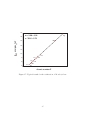
1
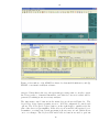
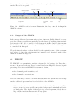
X-Ray Fluorescence (XRF) spectrometry for
materials analysis and “discovering” the atomic
number
Asma Khalid, Aleena Tasneem Khan and Muhammad Sabieh Anwar
LUMS School of Science and Engineering
June 28, 2011
X-Rays were discovered in 1895 by the German scientist, Wilhelm Conrad Roentgen. This discovery opened doors for the development of X-Ray Fluorescence
(XRF) spectroscopy which has now become a powerful and versatile technique for
the analysis and characterization of materials. It distinguishes different elements
present in a sample according to the characteristic X-ray energies emitted by them
and helps in determining their respective concentrations.
In this experiment we will use XRF spectroscopy to analyze a sample’s elemental
composition. From the characteristic X-ray energies, we will also verify Moseley’s
Law which is a proof of the existence of a fundamental quantity, the atomic number.
The atomic number increases in regular steps with an increase in the characteristic
X-ray energy. We will use this realtionship to find the Rydberg’s energy constant
and screening coefficient for Kα X-rays.
KEYWORDS:
X-Ray Fluorescence (XRF) · Characteristic X-Rays · Bremsstrahlung Radiations
· Moseley’s Law · Atomic number ·Screening coefficient · Rydberg’s energy·
APPROXIMATE PERFORMANCE TIME: 3 Week
1
Objectives
In this experiment we will,
1. differentiate between characteristic X-rays and Bremsstrahlung radiations,
2. use characteristic X-rays to identify elements,
1
3. acquire a spectrum, calibrate it and use it for qualitative (element identification) as well as quantitative (elemental concentration) analysis,and finally,
4. verify Moseley’s law and the validity of an atomic number.
References and Essential Reading
[1] http://www.dentallearning.org/course/AdvancedRadiography/
DoctorSpiller/x-ray_characteristics.htm
[2] http://hyperphysics.phy-astr.gsu.edu/hbase/quantum/xtube.html
[3] http://www.niton.com/portable-xrf-technology/how-xrf-works.
aspx?sflang=en
[4] http://www.sprawls.org/ppmi2/XRAYPRO/#BREMSSTRAHLUNG
[5] http://www.microsemi.com/micnotes/701.pdf
[6] http://www.byui.edu/physics/Thesis/Francom_Brian2008.pdf
[7] http://users.skynet.be/xray_corner/xtb/chap011.html
[8] H. Holbrow, N. Lloyd, C. Amato, E. Galvez, M. Elizabeth Parks, “Modern
Introductory Physics”, Springer New York Dordrecht Heidelberg London, pp.
536-542, (2010).
[9] S.B. Gudennavar, N.M. Badiger, S.R. Thontadarya and B. Hanumanaiah,
“Verification of Bohr’s Frequency condition and Moseley’s Law: An Undergraduate laboratory Experiment”, American Journal of Physics, 71, pp. 822825, (2003).
[10] P.J. Ouseph, K.H. Hoskins, “Moseley’s Law”, American Journal of Physics,
50, pp. 276-277, (1992).
[11] C.W.S. Conover and J. Dudek, “An undergraduate experiment on X-Ray
spectra and Moseleys Law using a Scanning Electron Microscope”, American
Journal of Physics, 64, pp. 335-338, (1996).
[12] Mini-X User’s Manual, Amptek Inc. (http://compassweb.ts.infn.it/
rich1/Stefano/Amptek_SW/Mini-X/Mini-X)
[13] X-ray detector (http://www.amptek.com/pdf/xr100cr.pdf)
[14] Digital Pulse Processor, Amptek Inc. (http://www.amptek.com/pdf/dp4.
pdf)
[15] Amptek Experimenter’s XRF Kit Quick Start Guide, Amptek Inc.
[16] http://www.dengeteknik.com.tr/veri/dosyalar/
metal-chip-nonferrous.pdf
2
[17] Amptek ADMCA: Display and Acquisition Software (http://www.amptek.
com/admca.html)
[18] Quantitative Analysis Software for X-ray Fluorescence (http://www.amptek.
com/pdf/fp.pdf)
[19] XRS-FP Quick Start Guide for Experienced Users, version 3.3.0, Amptek Inc.
[20] XRS-FP Software Guide, version 4.0.4, Amptek Inc. (http://
crossroadsscientific.com/Documents/XRS-FP\%20Software\%20Guide\
%20v404.pdf)
[21] Amptek K and L Emission Line Lookup Chart (http://www.amptek.com/
pdf/xraychrt.pdf)
[22] R.M. Rousseau, “The Quest for a Fundamental Algorithm in X-ray Fluorescence Analysis and Calibration”, The Open Spectroscopy Journal, 3, pp.
31-42, (2009).
2
Theoretical introduction
X-rays are part of the electromagnetic spectrum with energies ranging from 0.1 to
100 keV.
2.1
Production of X-rays
X-rays are produced by one of the three following mechanisms,
1. deceleration of high velocity electrons in the vicinity of a target nucleus,
2. atomic transitions between discrete energy levels, and
3. the radioactive decay of some atomic nuclei.
Each mechanism leads to a typical spectra of X-ray radiation.
2.1.1
X-ray tube
An X-ray tube is a device commonly used for the generation of X-rays by bombarding highly accelerated thermal electrons on a heavy metal target. It produces
X-rays incorporating the first two mechanisms.
A schematic for producing X-rays is shown in Figure 1.
1. A voltage is applied to the cathode which heats up the high resistance wire
filament. Electrons in the filament become excited and tend to boil off the
surface.
3
Cathode
Acclerated electrons
hitting the target anode
Heavy metallic target
Glass housing
Anode
Heated filament emits
electrons
Emiited X-rays
(Bremsstrahlung + characteristic
X-rays )
Figure 1: A simplified picture of an X-ray tube illustrating process of generating
X-rays.
2. A high voltage (in kilo volts) is applied across the gap between the filament
on the cathode and the heavy metal target acting as the anode of the system
which causes the thermal electrons to be attracted to the positively charged
anode. Due to high voltage, the electrons speed across the gap with tremendous velocity and finally hit the tungsten target so hard that they explode
into a shower of high energy photons. These photons are the X-rays.
The energy of the X-rays is controlled by the high voltage (measured in kilo volts,
kV) applied across the cathode and anode, while the intensity of the beam depends
on the number of electrons emitting off the filament. This number depends on the
temperature of the heating element which in turns depends on the current flowing
(in micro amperes, µA) through the filament. Increasing the X-ray tube voltage
results in both a higher X-ray intensity and a higher energy distribution. However,
increasing the X-ray tube current at a constant X-ray tube voltage increases the
X-ray intensity without affecting the energy distribution [1, 2].
2.2
Atomic processes involved in X-ray production
The production of X-rays by two different atomic processes, the X-ray fluorescence
and the bremsstrahlung radiation is discussed below.
2.2.1
X-ray fluorescence
X-ray fluorescence is the emission of characteristic or secondary X-rays from a
material that has been excited by bombarding with high energy electrons, or other
X-ray or γ-ray photons. If the incident particle has enough energy, it can knock
out an orbital electron out of the inner shell of the target atom. To fill the vacancy,
one of the electrons from the higher shells then jumps to the inner shell, emitting
4
in the process, a photon with energy equal to the difference in binding energy of
the two shells. The process is illustrated in Figure 2 (a).
The X-ray fluorescence produces an emission spectrum of X-rays at discrete energies. These emission spectral lines depend on the target element and hence are
called characteristic or fluorescent X-rays. We can use these spectra to identify the
elements by comparing the peak’s energy with the element’s binding energy [3].
Q 1. XRF can yield results only for elements with Z > 16 in air. Explain why
the lighter elements cannot be analyzed?
2.2.2
Bremsstrahlung radiation
Bremsstrahlung is a German word for braking radiation. Accelerating charges give
off electromagnetic radiation. In an X-ray tube, depicted in Figure 1, electrons
travel from cathode with high speed towards the anode and penetrate the anode
material. When these electrons pass in close proximity to the strong electric field
of the nucleus, they get deflected and are decelerated by the attractive force from
the nucleus, hence radiating X-rays, that are called braking or bremsstrahlung
radiation. The production of these X-rays is illustrated in Figure 2 (b).
This gives off a continuous distribution of radiation which becomes more intense
and shifts toward higher frequencies when the energy of the bombarding electrons
or the tube voltage (kV) is increased [4].
The bremsstrahlung spectrum can be described as follows.
An electrostatic field exists around the nucleus in which electrons experience the
braking force. The nuclear field can be imagined as a target with the actual
nucleus located in the center, as shown in Figure 3 (a). An electron striking
anywhere within the target experiences a braking force and produces an X-ray
photon. Now, the electrons striking closest to the center are subjected to the
greatest force and lose the most energy to produce the highest energy photons while
the electrons hitting the outer zones experience a weaker force and produce lower
energy photons. The outer zones capture more electrons and create more photons.
For this extremely simplified model, an X-ray energy spectrum is predicted to be
like the one shown in Figure 3 (a).
Q 2. Discuss the bremsstrahlung curve and its shape. From Figure 3 (b),
discuss the ideal and the experimentally obtained bremsstrahlung curves and comment on the reason for deviation from the ideal behavior.
The high-energy end of the bremsstrahlung spectrum is determined by the tube
voltage (kV) which establishes the energy of the electrons as they reach the anode.
Higher the tube voltage, greater would be the number and energies of electrons
striking the inner zones of nuclear force resulting in higher energy X-ray photons.
Q 3. In the spectra of Figure 4, distinguish between characteristic X-rays and
bremsstrahlung radiation. Why is the Figure (b) more spread out along the energy
5
(a)
Incident Primary X-ray
beam
Fluorescent
L X-ray
K
L
M
Ejected electron
Fluorescence
K X-ray
(b)
Scaterred electron
Incident electron
Bremstrahlung photon
Figure 2: X-ray emission through (a) fluorescence and (b) bremsstrahlung radiation. (a) illustrates the characteristic emission of K and L X-rays as a result
of electronic transition from L to K and M to L shells respectively, (b) shows a
decelerating electron emitting bremsstrahlung X-rays.
6
(a)
Counts / number of photons
Electrostatic field regions
around the nucleus
Energy (keV)
(b)
Counts
Ideal Bremsstrahlung curve
Experimentally
obtained curve
Corresponds to the
maximum voltage
set for the tube
0
0
Energy (keV)
Figure 3: (a) A model for bremsstrahlung production and the associated X-ray
photon energy spectrum, (b) an ideal bremsstrahlung curve shown as dashed line
compared to the experimentally obtained solid curve.
scale as compared to (a)?
The tube voltage also influences the production of characteristic radiation. No
characteristic radiation will be produced if the voltage is insufficient to overcome
the binding energy of the K-shell electrons corresponding to a threshhold voltage
as shown in Figure 4 (a) and (b).
2.3
Detection of fluorescent X-rays
The detection of X-rays is based on various methods. The most commonly known
methods in the past were photographic plates, Geiger counters and scintillators but
from 1970 onwards, semiconductor detectors have been developed and used, using
silicon or germanium as the detection elements. These detectors detect individual
X-ray photons that are reacting with the detector material. Each individual photon
is detected and then, over time, accumulated measurements make an accurate
picture of the radiation coming from the source.
7
Counts
29
22
14
6
(a)
5.61
11.32
17.03
22.75 keV
5.61
11.32
17.03
22.75
Counts
21
15
10
4
(b)
28.46 keV
Figure 4: Mini-X, X-ray tube output Spectrum with Ag as target anode (a) at
15 kV and 2 µA. Clearly the tube voltage is insufficient to overcome the binding
energy K-shell electrons and produce Ag Kα X-rays; (b) at 30 kV and 2 µA, the
spectrum shows a triangular bremsstrahlung continuous spectrum along with a
distinguished characteristic X-ray peak of silver near 22 keV
A PIN diode detector is today the most commonly used solid state X-ray detector.
It consists of an intrinsic semiconductor region sandwiched between a p-type and
n-type material, as shown in Figure 5. The X-ray photon enters the intrinsic region
and causes an avalanche multiplication of charges and the reverse bias field sweeps
the charges out of the region, resulting in a detectable and measurable current.
The mechanism of current production is illustrated in Figure 5. Each X-ray photon
absorbed in the detector creates an electron-hole pair. The ejected electron will
8
-
+
h
e
Characteristic
X-ray photon
I
P
N
Figure 5: A PIN diode detector. The characteristic photon produces a single
electron hole pair, if the electron produced has got enough energy, the charge keeps
on multiplying by collisions; e and h represent electrons and holes respectively.
possess an amount of kinetic energy equal to the difference between energies of
the incident photon and the band gap of the detecting material. This electron will
collide with other atoms and will cause further ejection of charge carriers in the
detector, producing an avalanche of charges. The migration of the electron and
holes takes place under the influence of a voltage maintained between the p- and ntype faces of the detector, which constitutes a pulse of current. The pulses created
are then amplified, recorded, and analyzed to determine the energy, number and
identification of the elements.
The sensitivity of these detectors is increased by operating them at low temperatures which suppresses the random formation of charge carriers by thermal vibration [5].
2.4
Energy dispersive X-Ray fluorescence (EDXRF)
A schematic representation of an EDXRF spectrometer setup is shown in Figure
6. The setup of EDXRF instrumentation is quite simple, consisting of four basic
components,
• excitation source,
• sample,
• detector, and
• data collection and analyzing system.
The EDXRF spectrometer helps plotting the relative abundances (in terms of
intensities) of characteristic X-rays versus their energy. The characteristic X-rays
generated strikes the detector element (in this case Silicon), creating an electron
9
Si detector and
preamplifier
X-ray tube
Multi channel
analyzer
Sample
Analysis
software
Element identification
and concentration information
Figure 6: The schematic of an EDXRF Spectrometer. The X-rays from the source
irradiate the sample, characteristic X-rays are detected by the Si detector, the multi
channel analyzer separates different elemental peaks and the analysis software gives
the final list of elements and their concentrations.
hole pair, which produces a charge pulse proportional to the energy of the X-ray.
This charged pulse is converted to a voltage pulse by a charge sensitive preamplifier.
A multi channel analyzer (MCA), is then used to analyze these pulses and sort
them according to their voltages. This data is then sent to the computer interface,
where it is displayed as the spectrum of the X-ray irradiated sample. The spectrum
is further processed to identify elements and quantitatively analyzed to find the
respective concentrations in a sample [6].
Q 4. What is a wave dispersive X-ray fluorescence spectrometer? What is the
difference between EDXRF and WDXRF and advantages of using one over the
other [7]?
2.5
Moseley’s Law
The power of XRF analysis was first realized by Henry Moseley in 1912, seventeen
years after Wilhelm Roentgen had discovered the X-ray.
2.5.1
A little bit of history: How atoms got their atomic numbers
Mendeleev’s periodic table of the elements was a significant advance in chemistry,
reflecting the similarities in the chemical properties of the elements and their periodic recurrence with an increase in the atomic mass. For over 40 years, the atomic
mass was a useful guide for scientists, but it provided no explanation for the periodicity of properties of the elements. During the early decades of the twentieth
10
century dramatic advances in physics revealed the structure of atoms and uncovered the physical basis of the periodic table. The atomic number was explained as
the number that specifies the position of an atom in the periodic table and is the
number of positive charges in the atomic nucleus.
The basis was laid in 1911 when Rutherford discovered the atom’s nuclear core after
which Bohr in 1913 showed that the nuclear charge Ze determines the scale of the
energy states of an atom. In the same year, Moseley measured the wavelengths of
X-rays emitted by many different kinds of atoms and showed that each chemical
element is uniquely identified by its nuclear charge. In other words, the nuclear
charge number Z specifies the position of an element in the periodic table and is,
therefore, the same as the atomic number which is the serial number of the element
in the periodic table. Hence the properties of X-ray line spectra were the basis of
Moseley’s discovery, and this is how elements got their atomic numbers !
2.5.2
X-ray line spectra
In 1905, a decade after Roentgen discovered X-rays, the British physicist Charles
Barkla found that a target struck by a beam of high energy X-rays (primary/incident
beam) emitted secondary X-rays distinctly different in behavior from those in the
incident beam. He discovered that the secondary X-rays emitted by a target are
unique to the chemical element the target is made of, so he called them characteristic X-rays, and pointed out that they could be used to identify the target
material.
Barkla had, infact, discovered a new means of chemical analysis. From his measurements of the absorption of X-rays Barkla found that an anode emits two distinctly
different types of characteristic X-rays, a more penetrating type (shorter wavelengths, higher energy) that he called K radiation or K X-rays, and a more easily
absorbed type (longer wavelengths, lower energy) that he called L radiation. These
emissions are called X-ray lines because they are analogous to the spectral lines in
the visible light spectra of atoms and are a unique fingerprint of the emitter atom
[8].
2.5.3
Mathematical formulation of Moseley’s law
Moseley studied X-ray line spectra and discovered a simple relationship that allowed him to predict the frequencies (energies) of X-rays for any element and to
see that the charge of the atomic nucleus is the property that gives an atom its
identity. Moseley after studying the X-ray line spectra in detail found that the
most intense short wavelength line in the characteristic X-ray spectrum from a
particular target element, called the Kα line, varied smoothly with that element’s
atomic number Z.
From Bohrs theory of atomic structure, something you have already studied in
11
your Modern Physics class, the energy of an electron in its orbit n is given by,
R∞ Z 2
,
n2
RE∞ Z 2
= −
,
n2
En = −hc
(1)
where h is Planck’s constant, c is the velocity of light, R∞ = 1.097 × 10⁷ m−1 is
the Rydberg constant for an infinitely heavy nucleus, RE∞ = hcR∞ = 13.06 eV is
Rydberg energy , Z is the nuclear charge, and n is the principal quantum number
used to designate energy levels.
The emission of radiation from the atom, according to Bohr, is due to the transition
of the atom from an initial higher energy state Ei to a final lower energy state Ef ,
and the frequency ν of the emitted radiation is given by the condition,
Ei − Ef = hν.
Now, a Kα X-ray emission is due to transfer of an L-shell (n = 2) electron to the
K-shell (n = 1), where a vacancy has been created by irradiating the atom with
incident X-rays prior to the transition. Hence the energy of the Kα photon is,
using (1),
(
EKα = −RE∞ Z
=
2
)
1
1
−
,
22 12
3RE∞ Z 2
,
4
(2)
which shows that the energy of characteristic Kα X-rays is proportional to square of
the nuclear charge. In the X-ray notation, the subscript α refers to the transitions
of electrons from L to K shell. A Kβ X-ray is emitted when electron jumps from
an M (n = 3) to the K shell.
Moseley, who was studying Kα X-ray spectra at the same time as Bohr, used
this expression, but modified Z to Z − 1 to fit to his experimental data. Thus,
Moseley’s relationship was,
EKα =
3RE∞ (Z − 1)2
.
4
(3)
The above equation is usually referred to as Moseleys law [9].
2.5.4
Effective nuclear charge and the screening effect
Moseley used Z − 1 instead of Z in (3) which is attributed to the fact that the
electron is not only attracted to the nuclear charge +Ze but is also repelled by
other electrons. Within a few years, this very idea had become commonplace in
12
the understanding of the multielectron atom, the true nuclear charge Z could be
replaced by an effective charge given by
Zef f = Z − ζ,
(4)
where ζ was called the screening constant [10, 11]: neighboring electrons “screen”
or “shield” the nuclear attraction. Thus, (3) could be modified to state that the
energy of an electron in a multi electron atom could be given approximately by,
EKα =
2
3RE∞ Zef
f
.
4
(5)
Q 5. Explain what does the screening factor indicate? Is there a way to determine this factor experimentally?
3
Description of equipment
Amptek’s XRF kit available and setup in our laboratory, is a package designed to
help the user quickly begin doing elemental analysis via X-ray fluorescence. Once
this kit is assembled and the software configured and calibrated, one can begin
doing simple analyses.
3.1
Amptek’s Hardware Components
The XRF kit includes,
• XR100 CR detector with Si-PIN diode,
• Mini-X USB controlled X-ray tube,
• PX4 digital pulse processor,
• XRF mounting plate,
• stainless steel SS-316 test sample.
3.2
Mini-X, X-ray tube
The X-ray source tube contains an electrically heated filament that generates electrons which are accelerated from the filament to the target Ag anode, by application of a high voltage. When these high velocity electrons are decelerated or
absorbed by the nuclei of the target atoms, bremsstrahlung or characteristic Ag
X-ray photons of high energy are produced. The Mini-X X-ray tube is fit with a
beryllium window, since beryllium is transparent to X-rays [12].
13
3.3
XR-100 CR, Si detector
This is a solid state silicon detector with a beryllium window. The window is
brittle and can be damaged beyond repair by mishandling. Make sure that
this window is not touched with anything at all, neither it is dropped or mishandled. The detector requires a very low operating temperature and therefore has a
thermoelectric cooling system. Touching the detector with bare hands will disrupt
this cooling system and damage it irreparably [13]. Always wear gloves while
handling the detector and be very careful during moving or positioning
the detector.
3.4
PX4: processor and analyzer
The Amptek PX4 [14] is an interface between Amptek’s XR100 detector and a
personal computer providing data acquisition and control, through analysis softwares. The PX4 is a component in the complete signal processing chain of the XRF
instrumentation system. It consists of a digital pulse processor (DP4), integrated
multichannel analyzer (MCA) and power supply.
The input to the PX4 is the preamplifier output from the Si detector. The PX4
digitizes the preamplifier output, applies real-time digital processing to the signal,
detects the peak amplitude digitally, bins these values in its histogram memory
and finally generates an energy spectrum. The spectrum is then transmitted over
the PX4’s serial interface to the user’s computer.
The digital pulse processor DP4 and MCA inside the PX4 unit have six main
function blocks to implement these functions, as shown in Figure 7. A detailed
description of MCA is described next.
DP4
|
Analog to
digital
convertor
Digital
shaper
Histogram
logic
Pulse
selection
logic
Power
supply
Figure 7: Block diagram of the PX4.
14
V
Analog
prefilter
|
Input from
detector &
preamplifer
MCA
Microcontroller
& interface
Computer
3.4.1
Multi channel analyzer and channel calibration
The characteristic X-rays are the main factor in realizing an XRF measurement
and it is essential to be able to accurately measure their energies. This can only be
achieved after a calibration of the detector and MCA has been performed. Once an
X-ray impinges on the detector, the detector sends an electrical pulse to the MCA.
The MCA will place each X-ray in its appropriate channel depending on the X-rays
energy. The data recorded is an array of numbers, each number representing the
total count of X-rays for that energy (intensity). The number placement in the
array represents the channel number, in ascending order as shown in Figure 8.
A calibration is a process in which specific energy values are assigned to the correct
channel in the MCA. This is done by sending X-rays of known energy values to
the MCA. Once the the channels where the X-rays were sorted are identified,
known energy values can be assigned to those channels. Since it is not practical
to assign energy values to each channel manually, the calibration process consists
of identifying two channels with known energy values separated by a large energy
and then applying a curve fitting technique to those data points. Through linear
approximation in this method, all the channels in the MCA can be indirectly
calibrated [6].
Si detector
Multi channel analyzer
0
9
8
1
1
2
5
7
0
(a)
Channels
Energy calibrated channels
1
2
3
4 ..............
1keV
......................
10keV .....
......
1024
40keV
Energy (keV)
A + Bx
Known element 2
Known element 1
(b)
Channel number
Figure 8: (a) Multi-channel analyzer (MCA) histogram memory representation.
The small boxes represent channels. The numbers represent a count of X-rays for
a specific energy, (b) linear calibration curve converting number of channels to
energy scale using two known X-ray peak enrgies
15
3.5
Radiation shield
Radiation safety is very important. The X-ray tube represents a personnel hazard
if it is not shielded properly. The shielding must prevent accidental personnel
exposure but must permit easy access to the samples. In addition the material
in the shield should not produce its own X-rays, since these would interfere with
measurements in the detector. The enclosure around the tube and detector must
stop primary and scattered radiation.
A cubical shield was designed with 0.25 inches brass as the inner walls of the cube
and 0.125 inches aluminum for the outer walls. Any backscattered X-rays absorbed
in the brass can produces Cu and Zn lines, which can be stopped easily by the
aluminum walls. The aluminum X-rays have a very short distance in air and hence
protect the experimenter and do not contaminate the measurement [15].
Q 6. How does the Si detector measures the energy of the X-ray photon?
3.6
Standard materials used in the experiment
We will use three kinds of standard reference samples in our experiment.
3.6.1
Stainless steel (SS-316)
The composition of the stainless steel alloy is given in the following table.
Cr
Mn
Fe
Ni
Cu M o
18.45 1.63 65.19 12.18 0.17 2.38
Table 1: Elemental composition (wt %age) of Amptek’s stainless steel standard
sample [12].
3.6.2
Chromium copper alloy (IARM-158B)
The composition of the chromium copper alloy is given in the following table.
Cr
Ag
Al
Fe
Mn
Ni
Pb
Si
Sn
0.85 0.01 0.002 0.09 0.019 0.32 0.01 0.02 0.01
Zn
Cu
As
C
Co
P
S
Sb
O
0.014 98.5 0.001 0.002 0.002 0.005 0.003 0.002 0.005
Table 2: Elemental composition (wt %age) of chromium copper standard sample,
obtained from Brammer [16].
16
3.6.3
Silicon brass alloy (31X-WSB7)
The composition of the silicon brass alloy is given in the following table.
Si
Zn
Cu
Al
Pb
Fe
Mn
Ni
4.25 7.581 72.74 3.87 0.025 1.95 03.39 3.03
P
Sb
Sn
As
Bi
Cd
Co
Cr
0.188 0.636 1.93 0.103 0.190 0.007 0.012 0.014
Table 3: Elemental composition (wt %age) of Si-brass standard sample, obtained
from Brammer [16].
4
Softwares for data analysis
In this experiment, the data will be acquired and analyzed using two kinds of
softwares, ADMCA 2.0 and XRS-FP.
4.1
ADMCA 2.0
The ADMCA program [17] is the main display and acquisition software. It is a
Windows software package that provides data acquisition, display, and control for
Amptek’s signal processor PX4.
4.1.1
Features
• It provides full control of all hardware features available in the connected
hardware (PX4 and detector),
• live display of the spectrum. Capable of displaying and calibrating up to
8142 channels of the MCA.
• Its spectral analysis features include
– energy calibration,
– setting up regions of interest (ROI), and
– computing ROI information (centroid, net peak area, FWHM).
• It also possesses an active link to the XRF-FP Quantitative Analysis Software
Package.
The ADMCA software performs the spectrometer calibration. The spectrometer
calibration refers primarily to the adjustment of the electronics (analog amplifier,
ADC and MCA) so that all peaks across a spectrum are located at their appropriate
17
(a)
(b)
Figure 9: Screenshots of (a) ADMCA software for elemental identification, and (b)
XRS-FP concentration analysis software.
energies. Unless this is the case, the spectrum processing cannot correctly convert
the X-ray peaks to elemental intensities, and therefore incorrect values will be
generated, resulting in incorrect assay analyses.
The important control buttons in the menu bar are shown in Figure 10. The
Acquisition Setup button permits access to all PX4 configuration controls and
options. The Gain Quick Adjust button on the right helps to quickly scale the
gain of the detector’s preamplifier. If the delta mode is enabled, the spectra do not
accumulate over time but a fresh spectrum is shown every second, which allows
one to see changes. The Def ine ROI and Calibrate buttons are used to perform
18
the energy calibration. Once a spectrum has been acquired, the data can be saved
and the file can be reopened.
Start/stop acquisition
Define ROI
Calibrate
Display
configuration
Acquisition setup
to configure PX4
Link to XRS-FP
software
Enable delta
mode
Auto tune
Gain quick
adjust
Figure 10: ADMCA window’s menu illustrating the key controls in Ampteks
ADMCA software.
4.1.2
Output of the ADMCA
In the energy calibrated spectrum with regions of interest (ROIs) defined for every
peak, the software searches automatically via the library (containing characteristic
peak energies of Kα , Kβ , Lα and Lβ for all elements from H to Fm) for the contents
of each channel that lies within the specified ROIs, which are then added together
to form the Peak Integral.
The peak integral values are then divided by the acquisition time of the spectrum
in seconds to produce the peak intensity in counts/second. A typical output of the
ADMCA is shown in Figure 11.
4.2
XRS-FP
The XRF-FP is a quantitative analysis software [18, 19] package for X-ray fluorescence. It processes the raw X-ray spectral data from Amptek’s detector, signal
processing electronics and ADMCA spectrum to obtain,
• the elemental peak intensities, and
• the elemental concentrations.
There are three major steps to an XRF analysis, after the system has been setup
and the calibrated spectrum has been loaded from the ADMCA.
1. Subtracts the detector’s response to recover the incident X-ray peaks. This
step corrects for escape peaks, sum peaks, background continuum and background peaks. The output of this step is a processed spectrum, ideally showing only the incident characteristic X-ray peaks.
19
(a)
(b)
Figure 11: (a) Output from ADMCA: Region of interest defined for the six selected
green peaks, (b) ROI detail, showing the initial and final positions for the each
peak, the centroids and the elements whose X-ray line exists at that centroid value.
2. Deconvolve the peaks to determine the intensity of the X-rays interacting in
the detector. The output of this step is a table of the intensities for each
peak to be analyzed.
3. Account for attenuation and matrix effects to determine the concentrations
of the elements in the sample. The output of this step is a table of concentrations, which is the final result of the analysis.
20
XRS-FP does the spectrum processing, requiring as input the parameters which
describe the spectrometer itself (e.g., the type, area, and thickness of the detector,
the distance between the tube and the sample, etc.) and parameters which control
the processing.
Figure 9 (b) captures a screenshot of XRS-FP window. Most of the parameters are found in the Setup menu item and are self explanatory. The parameters describing the detector are in Setup Detector menu. Some of the parameters for the X-ray source are in the Setup Source menu and others are in the
M easurement Conditions T able, which include the filter thickness, tube voltage
(kV) and tube current (µA).
Some columns of the Element T able are inputs while some columns of this table are
outputs (e.g. intensity, an output of spectrum processing). The Specimen Component T able
is used to select which elements will be analyzed. The Element T able is used to select which X-ray line is the basis of the analysis. The T hickness Inf ormation T able
is used to define the sample. The functions and processing of XRS-FP are explained
in the next sections.
Q 7. What are sum peaks, escape peaks and background peaks [20]? Why its
important to remove these peaks?
4.2.1
Spectrum processing in XRS-FP
An XRF spectrum consists of characteristic peaks superimposed on a background
(bremsstrahlung radiation and detector effects). It is the job of spectrum processing to effectively remove the signal (net peak intensity) from the noise (the
background peaks).
An additional complication is caused by peak overlap (the matrix effect). The
matrix effect is the absorption or enhancement of specific elemental X-ray peaks
by other elements present in the specimen. This effect hinders the simple method of
integration of regions around a peak to calculate the accurate elemental intensity.
To correct for the matrix effects, the XRS-FP software uses an empirical analysis
methods, called the FP calibration method which implicitly calibrate out the peak
overlaps and other spectrum artifacts to arrive at the true composition of elements
of a sample.
A brief introduction to the spectrum processing steps in place here.
• Element identification:
The element identification is required prior to extracting intensities. It is
implicit in this description that with every element there is a specified element that will be used for the final analysis. Using the Amptek ADMCA
application, the user can automatically mark peaks (ROIs) for analysis. If
the appropriate element library is loaded into ADMCA the software will associate the marked peaks with elements. The corresponding elements can
then be manually imported into the XRF-FP element table.
21
• Spectrum smoothing:
Smoothing of the spectrum is the first step in spectral processing. This operation typically performs a Gaussian smooth of each channel in the spectrum,
for the specified number of times.
• Si escape peak removal:
Escape peaks arise when internal fluorescence occurs, inside the detector
material (Si) and a fraction of a parent characteristic X-ray gets lost as SiKα escape photons, with an energy of 1.75 keV. Hence every feature in the
spectrum will have an associated escape feature at an energy lower by 1.75
keV. The software removes the escape peaks from the spectrum, and adds
the equivalent original X-ray event at the parent peaks energy.
• Sum peak removal:
Sum peaks arise because two incoming X-rays may arrive at the pulse processor within a time frame that is less than the minimum time interval required
by the detector to discriminate two events. This results in peaks that have
energies with the sum of the two incoming X-ray events. This correction is
not as accurate as the escape peak removal, and may leave some residual
sum peaks in the spectrum.
• Background removal:
The software uses the automatic background method to remove the background, which distinguishes fast-changing regions of the spectrum (peaks)
from slowly changing regions (background). The background curvature arises
primarily from bremsstrahlung X-ray continuum from an X-ray tube whose
shape depends on the anode atomic number and incident electron-beam energy.
• Deconvolution for Intensity extraction:
When the preliminary spectrum processing is complete, the net peak intensities must then be calculated.
Deconvolution is the process of assigning areas to the peaks of interest and
fitting the spectrum to a sum of separate peaks to calculate the net peak
intensities for the elements of the sample material. The Gaussian deconvolution method corrects for peak overlaps by synthesizing peaks for all the
expected lines (specified in the element identification step) in the region of
the analyte peaks, so that a complete peak fitting occurs for both the analyte
and the overlapping lines.
Gaussian method uses nonlinear fitting to give greater flexibility to the peak
deconvolution by allowing the peak ratios, widths and positions to change
in order to better fit the acquired spectrum. Gaussian peak profiles can be
adjusted in position, width and shape, which helps when there are changes
in the spectra from matrix effects, or changes in the X-ray spectrometer
performance (gain, offset and detector resolution).
22
4.2.2
Concentration analysis in XRS-FP software
Once the spectrum processing functions extract the peak intensities of all the
elements, the final step for the concentration analysis is carried out. The concentrations are calculated using the fundamental parameters (FP) function for the
quantitative analysis [19, 20]. This module solves a set of non-linear equations
which relate the intensity of the X-ray peaks to the concentration of the elements
in the sample. These equations include terms due to attenuation and enhancement (matrix effects) in the sample, attenuation in windows and air, tube spectra,
scattering of X-rays and thickness of filters used in the tube. For the XRS-FP
concentration analysis, one can choose either,
1. standard less method, or
2. FP calibration method.
In a standard less analysis, all of the parameters describing the X-ray tube spectra,
filtering, attenuation in air, attenuation in Be windows, attenuation and enhancement in the sample are computed from physical models based on the data the user
has entered into the software. It is simple to use standard less analysis but the
parameters are only approximate. This is due to approximations inherent in the
physical models and in the data entered by the user.
The FP calibration method, on the other hand, provides correction parameters
using either a single standard (reference sample containing known concentrations
of elements) or multiple standards (pure elemental standards). FP calibration is
strongly recommended and will lead to much more accurate analysis results. A
single type standard, i.e. a single material containing known elemental concentrations can be used with convenience. For example, one can use a stainless steel
SS-316 and then obtain very accurate analyses of other steel alloys or pure elements
containing at least one of the components of steel [19, 20].
The spectrum processing and concentration analysis carried out with the aid of
the two softwares ADMCA and XRS-FP, is conceptually illustrated in the Figure
12.
5
Experiment 1: Elemental analysis
In the first experiment, we will learn how to analyze a material sample to find its
constituent elements and determine their relative concentrations. We will start off
by obtaining the spectral data of a stainless steel sample (SS-316).
We have already seen in Section 2 that each element has a set of characteristic
X-ray peaks, unique in their energy. Therefore the peak energies can be used as a
fingerprint for element identification.
23
channel
to energy
Raw spectrum conversion
background and
escape & sum peaks
Processed
Energy calibrated removal
spectrum
spectrum
channel
Energy (keV)
Deconvolution
of peaks
Table of intensities
Matrix effect
correction by
standardless or
FP calibration
Table of conc.
Figure 12: Spectrum processing and concentration analysis steps carried out by the
ADMCA and XRS-FP softwares. The first two steps are performed by ADMCA
and the remaining ones by XRS-FP software.
5.1
Apparatus
We will use the Amptek’s XRF components listed below:
• X-ray tube (Mini-X),
• detector (XR-100 CR),
• digital pulse processor (PX4),
• ADMCA 2.0 software,
• XRS-FP software,
• base plate,
• sample mount,
• radiation shield.
24
5.2
Procedure
The assembly of the apparatus and its various components is shown in Figure
13. One should make sure that the PX4, X-ray tube and the detector are all
connected with the computer interface. The equipment manuals [12, 13, 15] should
be consulted for proper procedures and precautions.
Never switch the X-ray source ON without the shielding in place. Do
not expose yourself to direct or reflected X-rays. Do not touch the
X-ray tube when it is switched ON.
Do not touch the Be window of the detector. Be very careful while placing and mounting the detector, any sudden movement or the slightest
mechanical shock can damage the detector.
(a)
Base plate
9 V DC
Radiation
shield
9V AC/DC
adapter
110/220 VAC
Mini-X
Colimator and filter
X-ray tube
USB
HASP
plug
X-Ray
Radiation
Hazard
Sample mount
Sample
PX4
XR100 Si PIN
detector
USB
Digital pulse
processor
5 V DC
(b)
Brass-aluminum
shield
Sample
ADMCA software
Mini-X software
XRS-FP software
5V AC/DC
adapter
110/220 VAC
Mini-X
XR100
Figure 13: (a) Diagram of EDXRF spctrometer components connected to computer for spectral data acquisition and concentration analysis, (b) X-ray tube and
Si detector mounted on the base plate to irradiate the sample material. The
brass-aluminum box positioned to shield the experimenter from incident as well as
reflected X-rays.
25
Computer
5.3
Acquiring a spectrum in ADMCA
The stainless steel standard sample, SS-316 is mounted in the sample holder as
shown in Figure 14. The PX4 is switched on by pressing and holding the P ower
Sample holder
Shielding
base plate
Figure 14: Stainless steel sample mounted on the sample holder.
button on the front panel of the device for 3 seconds until the beep sound is heard
twice. Next, the ADMCA software is launched and from the DPP Dialog Box, the
option Connect to P X4 is selected. This will start the acquisition mode. Next the
X-ray tube is switched on using the following three steps:
1. The green safety interlock is plugged in carefully at the back of the tube as
shown in Figure 15(a). Next the adapter is plugged into the AC mains.
2. The Mini-X controller is launched by clicking on the Mini-X icon in the
taskbar and the Switchonthetube option is selected.
3. A voltage 30 kV and a current 30 µA is set and then the X-ray tube is
switched on by selecting the HV ON button on the software window, as
shown in Figure 15(b). A beep beep sound is heard a blinking red LED can
be seen at the rear end of the tube, which indicates that the tube is emitting
X-rays.
The Start acquisition tab is pressed and the spectrum is observed as it appears
on the ADMCA window. As soon as 100 counts are exceeded (the y-axis of the
spectrum is observed to keep track), the X-ray tube is switched off by using the
HV OF F control on the software window and then removing the power cable so
that the high voltage inside the tube is completely turned off.
The spectrum must be saved now in the ADMCA folder with the name steel.mca
and the spectrum window must remain open for the entire steps and subsequent
procedures described below.
Q 8. On the spectrum steel.mca identify the characteristic peaks. Use the
X-ray Chart [21] to identify peaks of Fe, Cr, and Mo.
Now, after obtaining spectrum with its peaks identified, the spectrum is showing intensity (counts) versus channels, which really is of no use to us. So this
26
(a)
(b)
30
30
30
30.0
30.0
Figure 15: (a) Safety plug inserted to complete the circuit for high voltage production in the tube, (b) USB controlled Mini-X’s software window to send the final
command to allow the X-ray emission.
spectrum should be calibrated to obtain graph between intensity (counts) and energy. This vital step of transforming channels to energy, called calibration, can be
subsequently used for qualitative and quantitative analysis.
5.4
Spectrum calibration in ADMCA with a standard sample
The ADMCA software is calibrated using SS-316, whose elemental composition
and concentration are provided in Table 1.
To start off, a few characteristic peaks need to be identified and given as reference
peaks to ADMCA for calibration. During calibration, care should be taken that
the reference peaks are such that a wide energy range is covered. For accurate
calibration, at least two peaks from the spectrum should be identified.
Two elements, Fe (at 6.40 keV) and Mo (at 17.48 keV) are chosen as reference
27
peaks. Fe is easy to identify as this will have the most intense peak in the spectrum,
having the highest concentration in steel. The peak of Mo is chosen as it lies in
higher energy range and is easily distinguishable, although of lower intensity, from
the rest of the spectrum.
Now the following steps are performed to complete the calibration.
• From the ADMCA window, the Def ine ROI command is selected which
opens another small window (an ROI is a group of channels around a peak).
To define an ROI, the cursor is first placed at the left and then at then at
the right edge of the peak, both values at the opposite ends will be displayed
under the start and end columns of the small ROI window. The Add button
is clicked to store the first ROI.
• The above step is done twice and ROIs are defined and stored for both Fe
and Mo peaks. The selected peaks will turn green.
• Next the toolbar button Calibrate is clicked to open the Calibration dialog
box.
• The dialog box is moved such that both peaks are visible and then cursor is
clicked on to the first peak. The peak should be highlighted in blue color and
the P eak Inf ormation section on the right-hand information panel should
be filled in.
• The Centroid button is then clicked on the dialog box. This will enter the
centroid value of the peak into the Channel memory. Then the energy value
of that peak is entered into the Value box (e.g., 6.4 for Fe) and then the Add
button is clicked. This procedure is illustrated in Figure 16.
• Now the cursor is clicked on to the second peak and its Centroid and energy
value (e.g. 17.48 for Mo), is also entered and added. The information for the
two peaks will then be shown in the box.
• In the U nits box the energy units (keV) are selected.
• Click OK.
• On the ADMCA window, the Enable calibration option is checked. This
command will convert the horizontal axis from channel to energy, hence we
finally see the intensity versus energy spectrum for the sample.
• Next the calibrated spectrum is saved with the name calibsteel.mca so that
we can use this calibration for element identification of unknown samples.
The V iew menu is opened andthe P ref erences option is selected, the file
path and file name are specified and the box checked for loading this calibrated spectrum every time, the ADMCA is run [17].
Our software and hardware has now been calibrated with the energy scale. We
can now use the software for qualitative analysis of any unknown spectrum.
28
Figure 16: The ADMCA display window showing the calibration dialog box.
5.5
Standardless quantitative analysis with XRS-FP
Before starting this section, students are strongly encouraged to refer to the XRSFP guide [19, 20] to have a detailed information of these parameters and their
effects on the analysis.
After successful calibration of the spectrum and qualitative analysis, we now move
onto quantitative analysis (calculating the elemental concentration by extracting
net intensities) of the sample, as discussed in Section 4.2.2. For this purpose,
the XRS-FP software is needed. The HASP plug available with the XRF unit, is
connected to the USB port of the computer and F P is launched from the taskbar
or the ADMCA window.
1. A yellow box appears with the version information. The box is clicked anywhere and another grey box appears. The Expert mode is selected and the
main screen pops up as shown in Figure 9 (b). The commands and controls
of the software have already been described in Section 4.2.
2. A new file is opened from the F ile menu and saved as steelanalysis.tf r.
3. The calibrated spectrum for the SS-316 sample is loaded into the XRS-FP
software from the Acquire menu.
4. Next from the XRS-FP Set up menu, we need to set all the parameters
defining the detector and X-ray tube types, the thickness of the detector’s
window, the filters used in the X-ray tube, the geometry in which the sample,
tube and detector are mounted. This information can be taken from XRF
maunals [15, 17].
29
5. The desired quantization mode (standardless or FP method) is selected from
the Quant option available under the Setup menu.
6. The sample’s geometry is defined in the T hickness Inf ormation T able.
Bulk mode is selected and the N ormalize option is checked to 100 in order
to get weight percentages of elements on a scale of 100.
7. The voltage and current values used for the X-ray tube are entered into the
M easuring & P rocessing conditions table.
After loading the spectrum into the XRS software and substituting all parameters
and selecting the standardless mode from the Quant menu, there remain three
major steps in a standardless quantitative analysis.
1. Element identification
Known samples: Elements present in the standard sample provided in
Tables 1, 2 and 3 are manually input to the Specimen Component T able
using the Insert key from the key board.
Unknown samples: Elements are identified from ADMCA by selecting
ROIs for all peaks. The ROI detail will provide the list of elements.
2. Spectrum processing: All the spectrum processing steps discussed in Section 4.2.1 are performed one by one by running the P rocess All command
in the XRS-FP window. The spectrum in ADMCA would now be a processed spectrum, with background and noise clearly removed from it. In the
Element T able of the XRS-FP window, the intensities against each elemental
line an be seen.
3. Concentration extraction: Finally the P rocess Analyze command is run,
which converts the intensities of each element into concentrations, using all of
the parameters input by the user to calculate and correct for the attenuation
and enhancement (matrix effects) in the sample from physical models and
mathematical equations [22].
5.6
Fundamental parameter quantitative analysis with XRSFP
It is simple to use the standardless analysis but the attenuation and enhancement
coefficients and hence the concentrations are only approximate due to approximations inherent in the physical models and in the data entered by the user.
With the FP analysis method, the correction parameters can be calibrated using either a single standard or multiple standards. Calibration is strongly recommended
and will lead to much more accurate analysis results. A single standard containing
multiple elements is convenient to use. In this Section, the SS-316 sample and
its calibrated spectrum calibsteel.mca already acquired and saved in the above
sections will be used and referred to.
30
5.6.1
FP analysis for stainless steel
After loading the calibsteel.mca spectrum into a new file of XRS-FP, saved as
F P calib.tf r and inputting all the parameters in the Setup menu, T hickness Inf ormation
and M easuring & P rocessing conditions tables, there are five steps (two additions to the standard less mode) that are followed for FP calibrated concentration
analysis.
1. Element identification: The known elements of SS-316 are entered to the
Specimen Component T able.
2. Initial estimates of concentrations: Against each element, the known
concentration values for each element from Table 1 are entered in the Specimen Component T able.
3. Spectrum processing: All spectrum processing steps are run to extract
intensities.
4. Calibration coefficients calculation: The Calibrate F P command is
run, which iteratively proceed and finally calculates the best estimates of
the calibration coefficients (or the sensitivity factors) for each element of the
stainless steel sample. The coefficients are displayed in the Element T able
against each element. Save this file again to save the calibration coefficients
into the F P calib.tf r file.
5. Concentration: Finally the P rocess and Analyze commands are run to
calculate the most precise set of concentrations for each of the elements of
the SS-316 sample, using the calibration coefficients and net peak intensities.
The resulting table of concentrations and coefficients achieved at the end of the
analysis is like the one shown in Table 4.
Component
Mn
Mo
Cu
Ni
Fe
Cr
Intensity
(c/s)
98.64
58.43
31.75
230.55
2162.29
1078.80
Line
Kα
Kα
Kα
Kα
Kα
Kα
Concentration
(wt %)
1.63
2.38
0.17
12.18
65.19
18.45
U ncertainty
(wt %)
0.16
0.31
0.03
0.79
1.38
0.55
Calib. coef f icient
7464.6
8165.6
38757.7
4586.4
5304.3
6856.5
Table 4: The concentration analysis of steel SS-316 completed through the XRS-FP
software. The relative intesnities and calibration coefficients are also listed.
5.6.2
FP analysis for unknown samples
The advantage of running the FP calibrated analysis is that now we are able to
find the precise concentration values for any unknown sample, containing any one
31
or some or all elements of the SS-316 in any weight percentage. Since we have
successfully calibrated the responses (calibration coefficients) of the elements of
steel i.e., Mn, Cr, Fe, Ni, Cu, Mo, we can use these response factors for any of
these elements whether they are present in a pure sample material or with other
elements in any sample and composition.
The analysis for an unknown sample, with any elements of steel, is outlined in
following steps.
1. The sample is mounted on the sample holder, while keeping the geometry of
the setup exactly the same as before.
2. The spectrum is acquired in ADMCA and ROIs are defined to get information
of the elements present in it.
3. The F P calib.tf r file, with a list of calibration coefficients, is loaded in the
XRS-FP software and the new spectrum loaded in to that file.
4. The spectrum processing steps are performed.
5. The Analyze command is run to find the concentrations.
Q 9. Obtain a spectrum of the Cu film provided and using the ADMCA and
XRS-FP softwares, perform the complete concentration analysis for the metal.
Q 10. Run a complete ADMCA and XRS-FP standard analysis for the Chromium
alloy IARM-158B as done for steel in Sections 5.4 and 5.6.1. Find the calibration
coefficients for all the elements of the alloy and their concentrations.
6
Experiment 2: Verification of Moseley’s law
In this experiment, Moseley’s Law is verified. The screening constant ζ for Kα
X-rays is also calculated.
6.1
Apparatus and Setup
1. X-ray Generator (Mini-X ),
2. Si X Ray Detector (XR100 ),
3. Digital Pulse Processor (DP4),
4. X-ray Shield,
5. Samples:
• stainless steel SS-316,
32
• chromium copper (IARM 158B),
• silicon brass (31X WSB7).
Always use gloves when handling these samples. Never touch them with bare
hands as this will contaminate the samples. Make sure the samples are placed in
the desiccator after use each time.
6.2
Procedure
• The apparatus is assembled as shown in Figures 13 (a) and (b).
• All the standard samples SS-316, IARM-158B and 31XWSB7 are used one
by one to have enough elements for the verification of the Moseley’s law.
• The sample is placed inside the shielding box with the flat surface facing the
source and detector.
• The spectrum will already be energy calibrated. (By initially setting the
preferences in ADMCA to load the calibsteel.mca file).
• The new spectra are saved.
Make sure you save all your spectra on the network drive.
6.2.1
Data analysis
1. The characteristic peaks of various elements are located in the sample. The
ROIs are used to look at the details. The spectrum can also be deconvoluted
in the XRS-FP software to distinguish between peaks.
2. A graph is plotted between the atomic number and the square root of peak
energies obtained from the ADMCA peak information. (MATLAB can be
used for data plotting.)
3. The slope and intercept of the plot are obtained and the uncertainties in the
values of both slope and intercept are also calculated.
The results of one such analysis is shown in Table 5. When we performed the
experiment, the energy of characteristic lines for each element were plotted against
their atomic numbers, yielding Figure 17.
Moseley’s law (3) is expressed as,
EKα =
3RE∞ (Z − ζ)2
,
4
33
Element Atomic number(Z)
Cr
24
Mn
25
Fe
26
Co
27
Ni
28
Cu
29
Zn
30
Ge
32
Mo
42
Ag
47
√
Kα enrgies (keV) Kα enrgies ( eV)
5.39
73.42
5.91
76.88
6.39
79.94
7.03
82.40
7.46
86.60
8.02
89.55
8.89
94.29
9.89
99.45
17.47
132.17
22.17
148.89
Table 5: The atomic number of elements and their corresponding characteristic
line energies obtained from standard samples SS-316, IARM-158B and 31XWSB7.
Taking square root of both sides, the equation becomes,
√
√
√
3RE∞
3RE∞
EKα =
Z−
ζ,
4
4
√
which resembles the equation of a straight line y = mx+c, with slope m =
√
and intercept c = − 3R4E∞ ζ.
3RE∞
4
Substituting the values of slope and intercept for this graph, and calculating uncertainties, we arrive at the values of Rydberg’s energy and scattering factor,
RE∞ = 14.33 ± 0.28 eV,
ζ = 1.60 ± 0.33 eV.
Q 11. Plot the graph of your values and discuss your results. Does your result
verify Moseley’s Law?
Q 12. Use your graph to calculate the value of the Rydberg’s constant and
scattering factor. How close is your value to the theoretical value of RE∞ = 13.60
eV?
Q 13.
Calculate the uncertainty in your calculated value of R∞ and ζ.
34
150
K energies eV
140
m = 3.28 + 0.02
c =-5.26 + 0.76
Ag
Mo
130
120
110
100
Ge
Cu
90
Co
80
70
20
Cr
Zn
Ni
Mn
Fe
25
30
35
40
45
50
Atomic number Z
Figure 17: Typical result for the verification of Moseley’s law.
35