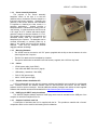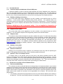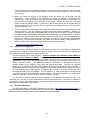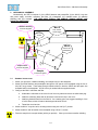
1
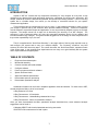
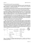
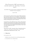
Amptek Experimenter's XRF Kit
Quick Start Guide
Characteristic
X-ray
Characteristic
X-rays
produced
EX-ra y =EK - EL
P rimary X-ray
M
L
K
Photoelectron
Collimator
and filter
Mini-X
X-ray Tube
Sample
Fe K⎯
Fe K⎯
Cr K⎯
Energy Spectrum
Measured
Ni K⎯
Mo K⎯
Counts
Mo K⎯
Ni K
XR100-SDD
Detector
0
5
10
15
20
25
30
Energy (keV)
Analysis
Results
Analysis Software
Processes Spectrum
Amptek, Inc
14 DeAngelo Dr, Bedford MA 01730
+1(781) 275 2242, www.amptek.com
Quick Start Guide – Introduction
INTRODUCTION
Amptek’s “XRF Kit” contains the key components necessary for X-ray analysis: an X-ray tube, a high
resolution X-ray detector with signal processing electronics, a baseplate to hold the tube, detectector, and
sample, software to control the tube and acquire data, and spectrum processing software. It is not a turn-key
system but is a flexible design, from which you can develop a customized solution for your specific
measurement application.
This kit requires two key components from you, the user: (1) the hardware necessary to hold or mount
your sample in position and (2) the enclosure which provides radiation shielding. These two components
must be tailored to a particular sample and application, so are not provided by Amptek, but they are critically
important. The sample mount has a major role in determining the accuracy of an XRF analyzer. The
enclosure is vital to personnel safety: the X-ray tube generates hazardous levels of X-ray radiation and
includes hazardous high voltages. This guide includes suggestions on the design of these components but
they are the responsibility of you, the user.
The kit is supplied with a “Quick Start Summary”, a two page outline of the key step required to set up
and configure your system and to carry out a sample analysis. The “Summary” contains a very brief
summary of each of the eleven key steps. The current document, the “Quick Start Guide”, expands on each
of the eleven steps. It also suggest some experiments one can carry out to gain familiarity with the system
and to explore different analysis options.
TABLE OF CONTENTS
1.
Equipment list and description
2.
Mechanical assembly
3.
Connect modules and install software
4.
Configure software
5.
Power up system and launch software
6.
System functional check
7.
Adjust and calibrate spectrometer
8.
Demonstrate spectrum processing
9.
Demonstrate quantitative analysis
Additional information can be found in Amptek’s application notes and tutorials. For those new to XRF,
several tutorials are likely to be of most interest:
X-Ray Emission Line Chart
X-Ray Fluorescence - A Description
X-Ray Fluorescence - Understanding characteristic X-rays
X-Ray Fluorescence - Advice for quantitative analysis
Once you have demonstrated the basic quantitative analysis described here, some advanced analysis
suggestions can be found in
Calibrating XRS-FP with chemical standards and using auto-mode
XRS-FP thin film measurement for lead in paint
1
Quick Start Guide – Introduction
WARNINGS AND PRECAUTIONS
These warnings and precautions MUST be read prior to installation and first operation. Serious
hazards exist in this equipment, some which are potentially LIFE THREATENING. Only qualified and
experience personnal should operate, maintain, or repair this system.
THE MINI-X GENERATES X-RAY RADIATION DURING NORMAL OPERATION AND PRESENTS
A SAFETY HAZARD. It must be used with radiation shielding (not supplied by Amptek) and
operated by qualified personnel. YOU ARE RESPONSIBLE FOR RADIATION SAFETY WITH THIS
SYSTEM.
The entire area around an X-ray system may represent a radiation hazard. Shielding, monitoring,
and safety interlocks are necessary for safe operation.
HIGH VOLTAGES ARE PRESENT IN THE MINI-X, THE XR100, AND THE PX4.
The Mini-X voltage is at a level which is potentially life threatening.
THE DETECTOR AND X-RAY TUBE BOTH CONTAIN THIN, FRAGILE BE WINDOWS. If the
windows are damaged, the units will be destroyed and cannot be repaired. Do not touch the
windows!
DO NOT DROP OR CAUSE MECHANICAL SHOCK TO THE XR100. Components inside the AXR
are mechanically fragile and may be damaged if the unit is dropped.
□
DO NOT REMOVE the red protective cap from the AXR detector until data are to be taken. The
detector window is made from thin beryllium (0.001 in / 25 µm thick) which is extremely brittle and
can shatter very easily. Do not have any object come in contact with the window. Do not touch the
window because the oil from your fingers will cause it to oxidize. The window cannot be repaired. If
the window shatters, the detector assembly must be replaced. Keep the red protective cover
nearby at all times and cover the detector when the instrument is not in use.
BERYLLIUM WINDOWS DAMAGED BY IMPROPER HANDLING WILL NOT BE COVERED BY
THE WARRANTY.
□
RADIATION DAMAGE to the detector will occur if it is exposed to a high flux environment.
Synchrotron Radiation Beams should be modified with attenuators before they are allowed to strike
the detector or the fluorescence target. Damage to the detector will be permanent if the flux from an
X-Ray Tube, a strong nuclear radiation source, or an accelerator is not attenuated.
A RADIATION DAMAGED DETECTOR WILL NOT BE COVERED UNDER WARRANTY.
□
No operator serviceable part are inside the XR100, the PX4, or the Mini-X. Refer servicing to
Amptek, Inc. To prevent electrical, shock do not remove covers.
□
For the latest information about this analyzer, including firmware upgrades, application software
upgrades, application information, and product information, go to
http://www.amptek.com/mcasoft.html
2
XRF KIT – GETTING STARTED
1
EQUIPMENT
Amptek’s “XRF Kit” is a package designed to help a user to quickly begin doing elemental analysis via
X-ray fluorescence. It includes hardware and software supplied by Amptek, which must be supplemented by
some components from the user. Once this kit is assembled and the software configured and calibrated, one
can begin doing simple analyses. This kit is general pupose, so is not tailored to a particular application, but
can be the starting point for a customized system.
1.1
AMPTEK COMPONENTS
Several Amptek supplied components are considered part of the kits. These are shown in Figure 1-1
and discussed in the sections below.
BNC Cable
Mini-X
X-ray Tube
5V AC/DC
9V AC/DC
USB Cable
LEMO Power
Cable
Mini-USB
Cable
Filter Kit
Collimator
Parts
Amptek
Installation CD
XR100
Detector & Preamp
Screws &
Washers
XR100
Spacer
PX4
Signal Processor
Baseplate
Figure 1-1. Photograph of Amptek components
1.1.1
XR100 X-ray detector and preamplifier
The XR100 includes the X-ray detector and
its preamplifier. As shown on the right, the
detector is a small diode mounted behind the Be
window on the front of the 1.5” extender.
There are several different detector
configurations sold by Amptek, optimized for
different applications. For general purpose use,
we suggest a 13 mm2 x 500 μm Si-PIN with a
multilayer collimator and a 1 mil Be window. For
options, go to www.amptek.com/xrselect.html or
contact Amptek, Inc.
Accessories can be fabricated by the
customer for use with the detector. These include
an external collimator, a shield (to minimize higher
energy radiation penetrating the sides of the
detector hybrid), or a filter. Dimensions are at
www.amptek.com/xrmech.html.
1-1
XRF KIT – GETTING STARTED
1.1.2
PX4 digital pulse processor and power supply
The PX4 interfaces between the XR100
detector/preamp and a personal computer with
data acquisition, control, and analysis software.
The PX4 includes three major components: (1) a
shaping amplifier, based on a state of the art, high
performance, low power digital pulse processor,
(2) a multichannel analyzer, and (3) power
supplies. It replaces both the separate shaping
amplifier, power supply, and MCA used in older
systems.
A photograph of the PX4 is shown on the
right. The PX4 is configured via software, using
Amptek’s ADMCA program. For further details on
the PX4, refer to the PX4 User’s Guide, on
Amptek’s Installation CD.
1.1.3
Mini-X X-ray tube and controller
The Mini-X (shown at top right) is a selfcontained, packaged, miniature X-ray tube
system, which includes the X-ray tube, the power
supply, the control electronics and the USB
communication to the computer. It features a 40
kV/100 µA power supply, a W or Ag transmission
target, and a Be end window. For further details,
refer to the Mini-X User’s Manual, on Amptek’s
Installation CD.
It is provided with a collimator and filters to
facilitate its use in XRF. As shown to the right, a
brass collimator (with aluminum insert) is retained
by a brass cover that screws into the Mini-X. An
aluminum insert absorbs characteristics X-rays
emitted by the brass. The collimator is 15 mm
long with a 2 mm diameter hole. A brass safety
plug is also provided which, when installed,
reduces the flux from an operating tube to less
than 2.5 mrem/hr. The units is shipped with the
brass safety plug installed, so the user must
unscrew the cover, remove the safety plug, and
install the collimator before use.
The user may fabricate custom collimators to
optimize beam geometry. A beam filter (which is
suggested) may be mounted inside the cover.
Amptek supplies a kit with several different
optional filters. We suggest a 10 mil (250 μm) Al
filter as a starting point but you should optimize
this filter for your application.
1-2
XRF KIT – GETTING STARTED
1.1.4
Sensor assembly baseplate
The purpose of the sensor assembly
baseplate, shown on the right, is to hold the
radiation source, the detector, and the sample in a
fixed and well known geometry. Optimizing the
geometry of the source, detector, and collimators
is important to obtaining the best results in a
particular applications.
Amptek provides a
baseplate which is intended as a starting point for
user tailoring. It holds the detector and source at
a 45° angle, for 67.5° incident and scatter angles,
and with a sample to detector distance of 1.6 cm.
The sample holder (supplied by the customer and
discussed below) must be mounted to the
baseplate by the customer. The baseplate can be
mounted horizontally or vertically (either up or
down), if the sample and its mount are properly
attached.
Note that the baseplate provides
negligible radiation shielding!!
1.1.5
Mounting Hardware
o
The XR100 must be mounted on a 0.375” spacer (supplied with the kit) so that the detector is at the
same height as the X-ray tube.
o
The Mini-X is attached to the baseplate by a bracket.
o
The spacer and bracket are attached used 4-40 screws, supplied, with a 3/32 hex key head.
1.1.6
Cables
□
XR100 power cable (6 pin LEMO)
□
Coax cable with BNC connectors (signal)
□
USB cables (1 standard, 1 Mini-USB)
□
PX4 +5 VDC power supply
□
Mini-X +9VDC power supply
1.1.7
Amptek software installation CD
A CD is shipped with the unit with all necessary software and detailed user manuals for each Amptek
item. Software includes the ADMCA software used for data acquisition and control, and the XRS-FP
software used for spectrum analysis. Several additional software packages and utilities are also supplied.
Software and manuals can also be downloaded from http://www.amptek.com/mcasoft.html.
1.1.8
HASP plug for XR-FP analysis software
The XRS-FP analysis software requires a HASP plug which must be inserted into the USB port of the
computer on which the analysis will be run.
1.1.9
Sample of stainless steel 316
A small piece of stainless steel 316 is supplied with the kit. This provides a material with a “known”
composition which can be used for initial testing and for calibration.
1-3
XRF KIT – GETTING STARTED
CUSTOMER SUPPLIED
1.2
1.2.1
Personal computer with Windows XP and 3 USB ports
A personal computer is used to control the data acquisition and control hardware and to analyze the
data. Any typical PC will function. It must run Windows XP or a 32-bit version of Vista. The 64-bit version of
Vista is not compatible with the USB drivers. It also requires at least 3 USB ports (one to communicate with
the PX4, one to communicate with the Mini-X, and one for the security plug of the analysis software).
1.2.2
Radiation shielding and enclosure
The section below offers some suggestions, but this is tailored to the particular items you will be
measuring. It must provide radiation shielding during normal operation. The materials used in its
construction should not be detected, since this would interfere with the measurement. The enclosure should
be easy to open, to put in samples, and should include an interlock so that the tube cannot be accidentally
energized.
Radiation shielding is vital to personnel safety. It is not supplied by Amptek but is
the responsibility of the customer!
1.2.3
Sample mount or holder
The section below offers some suggestions, but this is tailored to the particular items you will be
measuring. You must hold the samples in a fixed geometry relative to the tube and detector.
1.2.4
Samples to test
The customer must provide the samples to test and to calibrate the system. For initial setup and gaining
some experience, we recommend procuring metal alloys, of known composition, which are large enough to
cover the full beam area, flat, uniform, and thick enough to fully stop the beam. This will reduce many
difficulties which arise from thin materials, inhomogeneities, light elements, etc. Flat metal pieces can be
procured from many sources. For calibration, the best reference materials can be procured from NIST
(www.nist.gov/srm) but these are relatively expensive. Other supplies provide many additional and less
expensive reference materials.
1.2.5
Radiation survey meter
Used to verify your shielding.
1.2.6
Optional: oscilloscope
Although it is not required for setup or operation, an oscilloscope can be very useful for optimizing the
system, for debugging and trouble-shooting, and for visualizing system performance.
1.2.7
Optional:
55
Fe or 109Cd isotopic source
An isotopic source is not required, since the X-ray tube is the primary excitation source for XRF.
However, an isotopic source is often useful in debugging and trouble-shooting and as a reference. They are
convenient, if available. The 55Fe is useful because it is typically used to test XRF spectrometers and is the
reference used at Amptek so permits comparison with factory performance. The 109Cd is useful because it is
commonly used in XRF, since the Ag X-rays provide a good energy for measurements.
1.3
SUGGESTIONS FOR THE ENCLOSURE AND SAMPLE MOUNT
1.3.1
Enclosure and Shielding
The enclosure around the tube and detector must stop primary and scattered radiation, must minimize
scattering into the detector (which will interfere with a measurement), must permit the user to easily introduce
samples into the measurement chamber, and must ensure that the beam is off when the sample is changed.
Design of the enclosure is important to the customization of the system to a particular application and to user
safety, and for these reasons, the enclosure is the responsibility of the customer. We would offer some
general advice:
1. It is necessary to stop both the primary beam from the X-ray tube and also radiation which scatters in
all directions. The user must carefully measure for backscatter, even through small apertures. The
1-4
XRF KIT – GETTING STARTED
user must also check for radiation penetrating a benchtop or other components which one may
sometimes assume are a shield. Make extensive use of a radiation survey meter to verify the safety
of your setup!
2. When the X-rays are stopped in the shielding, some will scatter into the detector and any
characteristic X-rays produced in the shielding may reach the detector, contaminating the
measurement. Lead, for example, stops the beam but produces characteristic X-rays which will
likely interfere with measurement of elements in the sample. Amptek has found that 0.25” brass
usually provides an effective shield. It produces Cu and Zn lines, which can be stopped easily by
lining the brass with 0.125” Al, which does not contaminate the measurement (the Al X-rays have a
very short distance in air).
3. The user must open the shielding in order to place the sample in front of the tube and detector. This
raises two issues. First, the shielding must have some easy access mechanism. Second, it is
critical that the user only open this shielding when the X-ray tube is turned off. The Mini-X includes
an audible “beeper” and a flashing LED which indicate that X-rays are being produced. In addition,
the Mini-X includes an interlock which should be connected to the access. When the access port is
opened, the interlock is opened, turning off the beam. The Mini-X is shipped with a jumper across
this interlock. The interlock is described in more detail in the Mini-X manual. Further information on
radiation safety requirements for analytical X-ray instruments can be found at
http://www.crcpd.org/SSRCRs/hpart.PDF
1.3.2
Sample mount suggestions
To obtain accurate, quantitative results, it is vital that the geometry of the tube, detector, and sample be
unchanged from calibration to sample and from sample to sample. Even minor changes in the geometry can
have a surprisingly large impact on the measurement result.
The most important rule for XRF analysis is: Unknown samples and calibration samples MUST be
measured under identical conditions. X-ray fluorescence analysis is, as is the vast majority of other
analytical methods, a comparative analytical technique: one measures the intensity (count rates) of the
characteristic X-ray peaks of different elements; the concentration of the elements is deduced from the
directly measured intensity. The relationships between concentration of elements and measured
intensity depend on the conditions under which the spectra were taken. Therefore, the unknown
sample must be measured under the same conditions as the reference standards used to calibrate. A
comparative technique is only valid if the conditions are sufficiently similar to permit comparison. This is
the most important rule for XRF analysis. Violations of this rule lead to the most common and to the
most egregious XRF errors and mistakes. The first implication is: make certain that the same geometry
is used for calibration as for measuring unknown samples. The second implication is: use the same
equipment settings for calibration and for measuring unknown samples.
It is also useful to keep the sample as close as possible to the detector and to the X-ray tube. This
maximizes the count rate, for quick measurements, and minimizes attenuation in air, which is important at
low energies. Design of the sample mount is important in optimizing the system to a particular application
and thus is the responsibility of the customer.
1.3.3
Mechanical Drawings
The fabrication drawing of the MP-1 baseplate can be seen at http://www.amptek.com/mp1.html. It
includes some general purpose mounting holes, to which the sample holder and enclosure can be attached.
Additional holes or mounting hardware can be added by the user, as needed.
1-5
Quick Start Guide – Mechanical Assembly
2
MECHANICAL ASSEMBLY
Mechanically, the XRF kit consists of (1) the XR100 detector and preamplifier, (2) the Mini-X X-ray tube
with power supply, controller, collimator, and filter, (3) a baseplate, (4) a sample holder, (5) radiation
shielding, and (6) a sample. THE USER MUST SUPPLY THE SAMPLE, SAMPLE MOUNT, AND
RADIATION SHIELDING.!!
Radiation Shielding
Customer Supplied
Mini-X
X-ray Tube &
Power Supply
Collimator
& Filter
X-ray
Radiation
Hazard
XR100
Detector and
Preamplifier
Sample Fixture
Customer Supplied
Sample
Customer Supplied
2.1
ASSEMBLY INSTRUCTIONS
1. Mount your enclosure, radiation shielding, and sample mount to the baseplate.
2. Mount the XR100 detector and preamplifier through the 3/8” spacer to the baseplate using the four 440 (0.85” long) screws. These pass through clearance holes in both the XR100 and the space into
threaded holes in the baseplate. A 3/32 hex key is needed with the supplied screws.
3. Configure the Mini-X collimator and filter
a. Unthread the collimator cover at the front of the X-ray tube and remove the solid brass plug.
b. Install the collimator (brass with an aluminum insert and a hole) in the cover.
c.
Install any desired filters from the filter kit. As a starting point, we suggest installing 2 of the
10 mil Al filters, which will reduce the background below 20 keV.
d. Thread the cover back on.
4. Mount the Mini-X X-ray tube to its mounting bracket using two 4-40 (0.5”) screws
5. Mount the Mini-X and its bracket to the baseplate using 4-40 (0.5”) screws.
6. Place the sample in the sample holder (which you provide). Close your enclosure and/or shielding.
2-1
Quick Start Guide – Electrical Interconnects
3
3.1
ELECTRICAL INTERCONNECT AND SOFTWARE INSTALLATION
ASSEMBLY PROCEDURE
XR100
Mini-X
X-ray tube
Power
(6 pin LEMO)
9V AC/DC
Adapter
Signal
(BNC)
USB
PX4
Digital Pulse Processor
and Power Supply
USB
Computer
5V AC/DC
Adapter
Figure 1. Block diagram of electrical interconnects at the end of this procedure.
3.1.1 Connect PX4 and Install ADMCA Software and Drivers
1. Plug the 5VDC converter (round plug) into a 110/220 VAC outlet and into the back of the PX4.
2. Connect the USB cable from the back of the PX4 to the PC.
Figure 2. Photograph of PX4, showing front (left) and rear (right).
3. Turn on the PC and launch Windows (as an administrator). Insert Amptek’s installation CD.
4. Power on the PX4 by pressing the ON/OFF button (front panel) and holding it for about 3 seconds.
The PX4 should beep twice and the green button will be lit (it may blink….this is okay).
5. The “Found New Hardware Wizard” (shown below) should automatically appear when the PX4 is
connected and powered on for the first time.
6. Select “No, not this time” and click “Next>”.
7. Select “Install from a list or specific location (Advanced)” and click Next>.
3-1
Quick Start Guide – Electrical Interconnects
8. Select “Search for the best driver in these locations.” Then check the box “Include this location in the
search:” Select “Browse” and navigate to the \USB_driver\Win2K_XP folder of the Amptek
Installation CD. Click Next>. Note that the driver is actually called “Amptek DP4”.
9. Once the driver has been installed you will see the “Completing the Found New Hardware Wizard”
screen below. Click Finish.
10. Now that the USB driver is installed, browse to the Amptek Installation CD and copy the ADMCA
directory to the local computer, to C:\PROGRAM FILES\AMPTEK\ADMCA. Note that ADMCA cannot
be run from the CD; it must be installed on a local drive.
11. Browse to the ADMCA directory, right click on the Admca.exe file and select Create Shortcut. This
shortcut can then be dragged to the desktop. Launch the ADMCA software.
12. When ADMCA is loaded, a “Starting ADMCA” box appears. For now, click “Cancel”. Later, after the
system is completely connected and configured, you will connect to the PX4.
3.1.2 Install XRS-FP Analysis Software
13. Install the HASP into a USB port.
14. Locate the “Quantitative Analysis (XRF-FP)” folder on the Amptek Installation CD. Run “Setup.exe”.
and follow the directions. The ADMCA program must be running when the FP software is installed.
15. After FP is installed, close the ADMCA software.
3-2
Quick Start Guide – Electrical Interconnects
3.1.3
16.
17.
18.
19.
20.
Install Mini-X Software and Drivers
Note: Do not plug in the Mini-X until you have first installed the Application Software. This process
will also copy the USB drivers to your computer so that USB driver installation is easier.
Locate the Mini-X folder on the Amptek Installation CD. Run the “Mini-X Setup.exe” file.
When the dialog opens click “Next,” then click “Install,” then click “Finish.”
Another Wizard will open. Click “Next,” then click “Finish”. The application software is now installed.
Plug the 9VDC converter (rectangular) into a 110/220 VAC outlet and into the back of the Mini-X.
Connect the mini-USB cable from the back of the Mini-X to the PC.
Figure 3. Sketch of Mini-X connectors on the back of the unit.
21. When a new Mini-X is connected, Windows will prompt for the drivers to be installed. Select “Install
from a list or specific location (Advanced)” and then click Next.
22. Select “Don’t Search. I will select the driver to install” and then click Next.
23. Select Mini-X Controller A then click Next.
24. Click "Continue Anyway" to install the drivers. Repeat for Controller B.
Note: Steps 20 through 23 must be performed for every unique Mini-X (i.e. different serial number)
that is connected to the computer. The Mini-X USB interface contains two internal controllers, A and
B. This means that two USB drivers must be installed for each Mini-X. Perform the steps below for
both Mini-X Controller A and Mini-X Controller B.
3-3
Quick Start Guide – Electrical Interconnects
3.2
3.3
3.4
SAFETY NOTES
□
There are two screws which connect the metal backplate of the Mini-X to the cylindrical X-ray
tube in front. This provides the electrical return path (ground) for the X-ray tube’s high voltage
power supply. This connection is critical to safe operation!! If these screws are removed, then
the tube will float to potentially lethal voltages and represents a threat to personnel.
□
The back of the Mini-X includes an “Interlock” connector. The two pins of this connector must be
shorted together for the Mini-X to operate. The 9 VDC power to the HV power supply passes
through this connector, so if this is opened, the tube shuts down. For safe operation, this should
be connected to a switch which is integral to the radiation shield, such that the switch is opened
when the shield is opened.
□
THIS INTERLOCK CONNECTION SHOULD BE ATTACHED TO YOUR ENCLOSURE, FOR
PERSONNEL SAFETY. IT IS YOUR RESPONSIBILITY TO MAKE THIS CONNECTION.
REFER TO THE MINI-X MANUAL FOR MORE INFORMATION ON THE INTERLOCK.
□
The Mini-X includes a flashing red light and a beeper, both of which operate whenever the X-ray
tube is energized. These are important to warn operators of the radiation hazard.
GROUNDING NOTES
□
It is important, for safety, that the system be connected to earth ground. The AC/DC power supplies
are floating, with no ground connection. The ground connection could be made through the USB
connectors to the computer, which is then grounded.
□
We strongly recommend a separate ground connection. The back of the PX4 contains a ground
banana jack which may be used, or a wire can be connected to one of the threaded holes on the
baseplate. The most common cause of an ungrounded computer is a laptop which uses a floating
charger. If there are only two leads into the charger or the computer, it is not grounded. In this case,
a separate ground connection is necessary.
□
We have found some laptops which have particularly noisy charging circuits: they periodically inject
large current pulses into ground. This can interfere with the sensitive electronics in the XR100 and
PX4. If this is observed, we recommend floating the laptop charger and then making an alternate
single point ground connection.
□
If this sytem must be used in an environment with strong electromagnetic signals, then interference
may be an issue. The baseplate essentially ties all of the grounds together via a low impedance path,
so a single connection from any point on the baseplate to ground is usually best.
AUXILIARY CONNECTIONS
The connections described above are necessary for system operation. There are several auxiliary
connectors, which are not required for operation but which can be useful for debugging, for understanding
the system, and for accessing extra features.
3-4
Quick Start Guide – Electrical Interconnects
□
Analog Out: On the back of the PX4 is a BNC marked “Analog Out”. This can be connected to an
oscilloscope, where one can directly view the pulses. One can view the shaped pulses, or the fast
pulses used for pile-up rejection and measuring the input count rate, or the direct output of the ADC.
In ADMCA, under “Acquisition Setup”, the “Misc” tab permit one to select between them. The
ADMCA software includes an oscilloscope mode where one can see these pulses on a PC, but
connecting this to an oscilloscope provides a much better display.
□
Aux: On the back of the PX4 is a BNC marked “Aux”. This can display one of several digital signals,
selected from the “Misc” tab. The most useful is probably “ICR”, which indicates that a pulse was
detected in the fast channel. This can be used to trigger a scope or sent to a counter.
□
Digital I/O: On the back of the PX4 is a 16 pin D which contains a variety of signals. These are
documented in detail in the PX4 Manual. This includes a GATE signal, used to gate acquistion with
external hardware. It includes eight single channel analyzers, SCAs. Each SCA can be assigned a
lower and upper level, through software, and produces a logic pulse when an X-ray interacts with
energy between these levels. These can be connected to external hardware to read the count rate of
these channels directly. This also includes RS232 lines, for serial connection.
3-5
Quick Start Guide – Configure Software
4
CONFIGURE SOFTWARE
Each package of the software has its own configuration menus. Tailoring these settings is an important
part of tuning your system for your particular application. Because there are so many parameters, spread
over the software packages, it is often difficult for the novice to get started. We therefore provide an “XRF
Wizard”. This will provide a configuration which should work for simple analyses and will serve as a starting
point for more complicated analyses.
The Wizard’s first step is to find the all of the files needed by software, the executiables, .INI files, .CFG
files, etc. This is simple if you used the default directories suggested by the setup and installation utilities.
Some people choose not to use the defaults, or have multiple versions of the various files, in which case the
Wizard needs to locate the correct versions. The next step is to enter the critical data on the system – which
detector is used? what is the geometry? and so on. From these, the Wizard will select default options for all
of the different configuration parameters. Finally, the Wizard lets you view the parameters, and then
downloads them into the PX4 hardware and writes them into the .INI and other files.
4.1
USING THE WIZARD
1) Verify that the ADMCA, Mini-X, and XRS-FP software packages are all closed and that the PX4 has
been turned on.
2) Click on the “XRFWizard” icon or the .EXE in the
ADMCA directory. The screen shown to the right
appears. To select an item, click on the arrow.
When you have completed a step, the dot will turn
red. All steps must be completed to prepare a
configuration.
3) Click the “Find XRF Application Files” arrow. Some
users choose not to install the applications in the recommended
directories, or they install different copies in different locations. In
this step, the Wizard searches for the correct versions of the software
and for the setup and .ini files.
4) If you used the default directories during installation, then use the top
button, “Search in default locations”, on the page at right.
5) In the next page, shown below, make sure all three selections are
checked, then click “Default Search”. It will list in the three boxes the
paths to the files which were found.
6) Click Next. It shows the files and locations. Then click “Finish”. This
takes you back to the top menu.
7) If you chose not to install in default directories, then you will need to
use the “Advanced” selection, and in the next screen you must tell
the software in which directories to search. There are four steps on
this screen. In step one, check all three software packages.
In step two, you will define the scope of the search. If you choose
“Everywhere”, it searches throughout your hard drive, which can be
quite time-consuming. If you choose “Program Files”, then it will
search through the C:/PROGRAM FILES/ directory and
subdirectories. Alternately, you can click on the “Directory” button
beside each software package to tell the Wizard where to search for
that software.
4-1
Quick Start Guide – Configure Software
After you have defined the scope, click on “Search from specific locations”. The software will display
all copies it finds of the three software packages (some users have multiple copies installed).
Double-click on the copy you wish to use, for each of the three packages, then click “Next”
8) Click “Detector Properties”. It asks if you have an Amptek
detector. If you are using this kit, you are using an Amptek
detector, so say “Yes”. It will display a list of the most
common Amptek detectors. Along with your detector,
Amptek provided a data sheet, showing an 55Fe spectrum
(a sample is shown to the right) At the bottom of this sheet
is text which states the type of detector shipped and the
thickness of the Be window (circled in the sample below).
Select the Amptek detector and window, then click “Next”.
[Note: If you are not using a detector from Amptek, you will
need to use the “Setup Detector” menu in XRS-FP. The
detector vendor will provide you the data needed].
9) Next, select which of the three signal processing
electronics options you purchased (an X-123 with SiPIN
or CdTe, an X-123SDD for a drift detector, or a PX4 for
either).
If the PX4 is turned on, as we strongly
recommend, you can click “AutoDetect” and it will find the
hardware and its status. Click “Next” and return to the
main menu.
10) Click “Setup Source”. The menu shown to the right
appears. The standard XRF Kit from Amptek is supplied
with a Mini-X X-ray tube, with either an Ag or W anode.
Amptek also sells the Eclipse 4 small X-ray tube. You
may select one of these options, or else choose a 57Co or
109
Cd isotopic source. If you have a different tube or
source, use the “Setup Source” menu within XRS-FP
rather than this Wizard to configure the system.
11) Click “Next”. If you selected a tube, then the screen on the
left below appears to let you enter information on any filter
you plan to use with your tube. The Mini-X is shipped with
a filter kit. If you will make your filter from this, click “YESAmptek Filters”. The screen on the right below appears,
showing the different filters in the click. Enter the correct
number for the filters you will use, e.g. 2 layers of 254 μm
(10 mil) Al. We recommend 2 layers of 10 mil Al to start.
Click “Next” and enter the voltage and current you plan to
use for the tube. Click “Next”.
4-2
Data sheet
Key parameters
Quick Start Guide – Configure Software
12) Back at the main menu, click “Setup Geometry”. The
first question is “Do you have Amptek’s standard
baseplate?” This is shipped with the XRF Kit, so if
you will use this, select “Yes”. The software will
display the sensor head geometry and the default
geometric quantities needed by the analysis
software. If you are using your own sensor head,
use the picture to enter the appropriate values. Click
“Next”
13) You should now have the screen displayed on the
left below, where the first four buttons are green. Click “XRF Configuration Summary”.
14) The screen on the right above appears. This gives you the chance to view the configuration settings
and then to save them. Click “Save Old Settings and Install New Settings”. An .HTML file is opened
which contains all of the parameters. There is a table of detector parameters for XRS-FP, a table of
settings for the PX4, and so on. The software then writes new values into the appropriate files (a .INI
file and a .TFR file for FP, a Wizard.CFG file for PX4) and into the PX4 hardware. Then click Finish.
4-3
Quick Start Guide – Configure Software
4.2
SUGGESTIONS FOR ADVANCED SETUP
For the novice user taking his or her first
spectrum, we recommend using the defaults set by
the Wizard for your first analyses. However, you will
certainly want to tweak these values later, to optimize
the system. If you obtained a nonstandard system,
then you may need to set non-default values.
ADMCA controls the parameters used by the
digital processor: the gain, the peaking time, the high
voltage bias on the detector, the acquisition time, etc.
Within ADMCA, click on the “Acquisition Setup”
button and you will see the page displayed on the
right. The tabs permit you to access related sets of
parameters. Of most importance:
MCA: This tab lets you set the acquisition time (e.g.
60 sec), along with the number of channels in the
spectrum and the LLD on the spectrum.
Shaping: This tab lets you set the peaking time. In
general, short peaking times permit one to operate at
high count rates but degrade energy resolution. This
tab also lets you set the baseline restorer parameters
(which stabilize the spectrum) and the fast threshold,
used for counting the incoming counts and in the
pile-up rejection logic.
Gain and Pole-Zero: The gain is quite important. It can be set using buttons at the right of the toolbar or
here. The other parameters on this page do not often need adjusting.
Power: This permits one to set the HV bias and also the detector temperature. You get the best
performance if the detector is cold, but if the detector temperature changes, then the gain of the system will
change. Set the detector temperature so that, under the warmest ambient conditions you expect, the
temperature is regulated.
Misc: This tab should not be needed under normal conditions. It controls the AUX outputs (on the back of
the units) and has an “Oscilloscope” mode where pulse shapes are displayed on the computer.
4-4
Quick Start Guide – Configure Software
XRS-FP does the spectrum processing and so contains all the parameters needed for this. It has
parameters which describe the spectrometer itself (e.g. the type, area, and thickness of the detector, the
distance between the tube and the sample, etc) and parameters which control the processing (how to
smooth the spectrum, if sum peaks are removed, what peak shape model to use, etc). Parameters
describing the spectrometer usually have a single, correct value – there is only one right value for the
detector thickness, shaping time, etc. However, the process parameters do not have unique values.
Instead, they can be adjusted to provide the best results for your application.
The screen below shows the main screen. Most of the parameters are found in the “Setup” menu item
and are pretty obvious. The parameters describing the detector are in “Setup Detector”, for instance. Most
of the parameters for the X-ray source are in the “Setup Source” menu, but some are in the “Measurement
Conditions Table”, e.g the filter thickness and beam kV and uA. Some processing parameters are found in
“Setup Processing” but others are found in the “Element Table” below. Some columns of the “Element
Table” are inputs (e.g. the intensity method, where one can choose a Gaussian deconvolution or other
options) while some columns of this table are outputs (e.g. Intensity, an output of spectrum processing).
As is described later in this guide, some key parameters must be entered into XRS-FP and not by the
Wizard: the parameters relating to the sample. The “Specimen Component Table” is used to select which
elements will be analyzed. The “Element Table” is used to select which X-ray line is the basis of the
analysis. The “Thickness Information Table” is used to define the layers of the sample: Is it a thick,
homogeneous, bulk sample, or a thin but homogeneous sample, or are there coatings on a substrate?
This is a very brief introduction to the configuration parameters in the software! These parameters are
described in the manuals and user’s guides supplied with the software. We also provide an application note
which has background information on XRF spectra and spectral analysis software. Our suggestion is that,
after you have successfully walked through this manual and carried out simple analyses, you refer to these
manuals and empirically adjust parameters to optimize the system.
4-5
Quick Start Guide – Power On and Launch Software
5
5.1
POWER ON AND LAUNCH SOFTWARE
START UP PROCEDURE
1. Press the power on button on the front of the PX4 and hold it on until the PX4 beeps twice (the
second beep takes about 3 sec). If you only hear one beep, then turn the PX4 off and try again.
Waiting for the second beep loads the last configuration.
2. Double click the “ADMCA” icon on the desktop. When the “start box” appears, select “PX4”, then
click the “Connect” button.
Figure 5-1. ADMCA Start up screen.
3. After the software has connected to the PX4, it will look as in Figure 5-2. Specifically, there will be a
green USB logo on the bottom right. It will show the PX4 serial number at the top right, with
appropriate status and configuration data as well.
PX4 S/N
PX4 Status
USB Logo
Figure 5-2. ADMCA screen after connecting to the PX4.
5-1
Quick Start Guide – Power On and Launch Software
4. Double click the “Mini-X” icon on the desktop. The screen shown below will appear. Click the “Start
Mini-X” button at the top.
Figure 5-3. Mini-X Start up screen.
5. Once the software has connected to the Mini-X, it will appear as in Figure 5-4 The serial number will
appear at the top, and the “HV On” and “HV Off” buttons are available. If the safety interlock is open,
then this will be shown in the screen.
Figure 5-4. Mini-X screen after connecting to hardware.
5-2
Quick Start Guide – Power On and Launch Software
5.2
ADMCA SOFTWARE
The software is described in detail in the manuals supplied on the installation CD and also in the “Help”
menu. The documentation in the “Help menu is the best reference for the ADMCA software. There are a
few key buttons, which are most often used.
Start/Stop
Acquisition
Acquisition Setup Button
Click here to configure PX4
Define ROI
Enable Delta
Mode
Calibrate
Display
Configuration
Auto
Tune
Gain Quick
Adjust
Figure 5-5. Drawing illustrating the key controls in Amptek’s ADMCA software.
The buttons across the top shown here are the most important for the steps discussed here. The
“Acquisition Setup” button permits access to all PX4 configuration controls and options. The “Gain Quick
Adjust” buttons, on the right, let one quickly scale the gain. It is convenient to enable “delta mode” during
initial set-up and check-out; in this mode, the spectra do not accumulate over time but a fresh spectrum is
shown every second. This permits one to quickly see changes. We strongly recommend using “Tune
Fast/Slow Thresholds” once all parameters are set.
“Start/Stop Acquisition” is clearly important The “Define ROI” and “Calibrate” buttons are used to
perform an energy calibration. Once a spectrum is acquired, the data can be saved and the file reopened
using the WindowsTM standard Save/Open button.
5-3
Quick Start Guide –Functional Check
6
SYSTEM FUNCTIONAL CHECK
At this point, the system has been complete assembled, configured, and powered up. It is now time to
turn on the X-ray tube and acquire a spectrum from the detector. The goal in this step is verifying that it
functions at all and verifying the safety of the radiation shielding. In the next step, we will tune the
configuration and verify the performance.
6.1
1.
2.
3.
4.
5.
6.
6.2
CHECK X-RAY TUBE AND SHIELDING
Verify that the shielding is installed. Verify that a sample is in the sample mount.
Turn on the radiation survey meter and check it. Use the battery test, and if possible, use a known
source to stimulate the survey meter.
Verify that the tube is set to 15 kV and 15 uA. This is starting at a low level for safety sake.
In the Mini-X software, click “HV On”, then select “Yes” on the box that appears in a couple seconds.
The Mini-X should begin beeping, a red light on the unit will flash, and a symbol will flash on screen.
Use the survey meter to verify that the shielding is effective. Scan all the way around the assembly,
checking particularly for scattered radiation.
CHECK THAT THE X-RAYS ARE DETECTED
1. In the ADMCA software, start an acquisition by pressing the space bar or clicking the “Start” button on
the toolbar.
2. A spectrum should begin appearing. The figure below shows the spectrum from steel, after a minute.
Your spectrum won’t look just like this but there should be a spectrum accumulating. The green bar
at right will show the time and total counts accumulating. A small green box at the lower right shows
that the USB connection is good.
3. If you see the counts accumulating, distributed along the horizontal axis, the system is working
properly. If no counts are seen or if there is only a “blob” at the left end of the horizontal axis, or if the
green USB signal keeps turning red and you drop connection, refer to the trouble-shooting guide.
6.3
RADIATION SAFETY CHECK.
1. Increase Mini-X HV setting to 40 kVp (maximum). Use the survey meter to verify that the higher
energy radiation is stopped by the shielding.
2. Increase Mini-X current to 100 uA (maximum). Use the survey meter to verify that the higher energy
radiation is stopped by the shielding. Check in all directions.
6-1
Quick Start Guide –Functional Check
SPECTOMETER OPERATIONAL CHECK.
6.4
The goal of this next step is to make sure that the gain, energy resolution, and Mini-X bias voltage are
all in reasonable ranges. You want to make sure that the spectrum “makes sense”. It is simplest to use the
major X-ray line in your sample and then scale from this. For those unfamiliar with checking these
parameters, the next steps describe a simple check which was performed with stainless steel 316.
Sample Spectrometer Check
Figure 1. Spectra taken from a stainless steel sample Data were taken at 30 kVp and 30 uA.. The plots
show the same spectrum, but the one on the left (right) is in a linear (logarithmic) scale. The highest peak is
the Fe Kα peak at 6.4 keV. The isolated peak in the middle of the spectrum is the Mo Kα peak at 17.44 keV.
These two are very convenient for calibration and scaling.
1.
With the shielding in place, set the Mini-X to 30 kVp and 30 uA. Turn on the HV, clear the data in
ADMCA, and acquire a spectrum.. To acquire the spectrum, the “Start/Stop” button was clicked,
then the “Delete data and reset time” button was clicked (you can also use keyboard shortcuts:
press the spacebar to start acquisition, and press “A” to clear dat and time). After a minute or so,
click the “Start/Stop” button to stop.
2.
Place the cursor on the largest peak (the one with the most counts). Note: T to go between linear
and log scales, use the “Display”, “Scale” menu. In the example above, the Fe peak (6.4 keV) is
about channel 359. The horizontal axis extends to channel 2048, or almost 5x the Fe peak, thus
approximately 40 keV, which is the full scale energy. This is a reasonable starting point.
3.
Use the “right arrow” key at bottom right to zoom in at the cursor location (which should be the Fe
peak). The plots above show the zoomed display around the Fe peak. Each peak is well
separated, with a deep valley between the peaks. This indicates good energy resolution, i.e. low
noise. A poor energy resolution is indicative of an improper configuration.
6-2
Quick Start Guide –Functional Check
4.
6.5
On the toolbar, click on the “Full Horizontal Range” button to zoom out fully. Place the cursor at the
upper end (along the horizontal axis) of the “bump” seen in the middle of the spectrum (log scale is
needed to see this). This bump arises from the brehamstrahlung continuum emitted by the tube,
backscattered from the target. The upper end is at channel 1550, which is around 28 keV. This is
consistent with an HV setting of 30 kVp.
EQUIPMENT FAMILIARIZATION
If you are unfamiliar with the spectrometer and the software controls, this is a convenient time to gain
familiarity. The following steps will show how to carry out the most common functions. Note: If you hold the
mouse over one of the toolbar buttons in ADMCA, a label appears with the name of the box. If you open
Help Topics, the software manual is available and will explain these functions in more detail.
1. With the radiation shielding in place, turn on the tube. Click the “Delta” button on the toolbar. This
enables “delta” mode, in which the data do not accumulate over time. Every second, a spectrum is
acquired and shown, then a new spectrum is shown the next second. This mode is convenient to use
while you are setting up the equipment, since it makes it easy to see changes.
2. Click the “Increment gain by delta” button, at the far right of the toolbar. The spectrum should “scale
right” as the gain is increased. Click the “decrement gain” button to shift the spectrum to the left.
3. Click the “increment gain” button several times. If the gain increases enough, you should start to see
a large tail of counts at the lowest channels. These are noise counts. When the gain increases
enough, the noise starts to exceed the threshold and so these counts appear. Turn off the tube,
using the Mini-X software, and click the “Tune Fast/Slow Thresholds” button. The thresholds are
automatically adjusted above the noise. In the “information pane” on the right, verify that the count
rate is under 5 per second.
4. Turn the Mini-X back on, at a low current. In the Info pane, verify that the Dead Time is low (<10%).
The pane shows “Counts” and “Input Counts”. The “Counts” value shows the number of counts which
are processed in the main channel. Due to pulse dead times, some pulses will be not be recorded,
so the “Input Counts” should be a little higher than “Counts”.
5. Take a spectrum with a sharp peak, such as the copper spectrum above. Stop acquisition and turn off
the tube. Click the “AutoScale Vertical” button on the toolbar; this will adjust the vertical scale so the
peak counts are near the top. Using the mouse, click somewhere near the peak. Press “L” to toggle
between linear, logarithmic, and square root vertical scales (in the “Select” pane at the bottom of the
screen, towards the right, the software displays which scale has been chosen). The linear scale
makes the major peaks clearest, while the log scale makes the spectral background clearest.
6. “Regions of interest”, or ROIs are important for analysis. An ROI is a group of channels around a
peak. To define an ROI, first click near a peak to be analyzed. Then zoom in by clicking the “>”
arrow located towards the lower right of the “Select” Pane. Next, click the “Edit ROI” button on the
toolbar. Place the cursor over one edge of the ROI, depress the mouse button, and keeping the
button depressed, drag the cursor across the peak, and the release the mouse button. The figure
below shows an ROI defined around the Fe Kα peak in the spectrum above.
6-3
Quick Start Guide –Functional Check
7. In the “Info” pane to the right, there is a section called “Peak Information”. This has important data
regarding the peak defined by this ROI. This includes the centroid and the width (specified as full
width at half maximum). Since the energy scale has not been calibrated, these will appear in units
of “channels”. Also shown are the “net area” which is the number of counts after a simple
background removal, and the net rate, the net area divided by the measurement time. Select the
“Full Horizontal Range” button on the toolbar to see the whole spectrum again.
8. Click the “Display Settings” button to see the PX4 hardware settings. Click the “Acquisition Setup”
button, which will bring up a box with many tabs. This permits access to all of the hardware settings
for the PX4. These can be used to optimize settings for the very best performance.
9. Close this box and restart data acquisition in delta mode. In the Mini-X software, increase the high
voltage setting. The upper end of the continuum should move up in energy. Increase the current,
and verify that the count rate scales proportionally.
6-4
Quick Start Guide –Adjust and Calibrate
7
7.1
ADJUST AND CALIBRATE SPECTROMETER
ADJUST SPECTROMETER
The configuration selected by the Wizard was chosen to be a good starting point for most analyses but
can almost certainly be optimized. In this step, we will suggest the most important adjustments.
1. The most important parameter to adjust is the gain. The gain should be set so that the highest
energies to be analyzed appear near the upper end of the energy scale. In the default settings used
here, the upper end of the spectrum should be around 40 keV. If the highest line to be analyzed is
Zn, at 9.57 keV, increase the gain to give 12 keV full scale. This is the optimum combination of
resolution and dynamic range. Use the “Increment gain” or “Decrement” gain buttons on the toolbar
to obtain the desired energy range.
2. The Wizard sets the peaking time to obtain the optimum energy resolution, which usually implies a
long peaking time and therefore low count rates. In many applications, one needs high count rates.
Use the “Acquisition Setup” button and the “Shaping” tab to adjust the peaking time. At very high
count rates, it may be useful to reduce the “Detector Reset Lockout Period” on the “Gain and Pole
Zero” tab.
3. Once all the other parameters have been set, we strongly recommend tuning the thresholds using the
“Tune Fast/Slow Thresholds” button on the toolbar. Note that tube should be turned off before this is
set. Note: while the system is being configured, it is possible to have the system triggering on noise
counts. If the fast channel is triggering on noise, and pile-up rejection (PUR) is enabled, all counts
will be vetoed. It may prove useful to disable PUR while parameters are being adjusted, and then to
enable it again before starting data acquisition.
7.2
CALIBRATE SPECTROMETER ENERGY SCALE
Once the spectrometer is adjusted, the energy scale must be calibrated. The PX4 is a pulse height
analyzer, where the height of each pulse is proportional to the deposited energy. The proportionality
depends on the gain and on many parameters, so each system must be calibrated. One needs to acquire a
spectrum with a few peaks at definite energies, and then the software performs a linear regression.
1. Turn off the Mini-X and install a sample with known composition. Calibration requires at least two
peaks, preferrable well separated in energy. It is best to acquire at least 50,000 counts in each
photopeak (net area). One can use a single sample with several peaks or can take several spectrum
from single element standards or radioisotopes.
2. Define regions of interest around the peaks of known energy. The sample below is of steel, with the
Fe and Mo peaks selected.
Figure 7-1. Screen captures showing the calibration process.
7-1
Quick Start Guide –Adjust and Calibrate
3. Click the “Calibrate” button. The box shown on the right will appear.
4. Place the mouse over a particular peak and click anywhere with the region of interest. In the
“Calibrate” box, click “centroid” and the peak’s centroid is entered into the channel box. Click the
“Value” box and enter the known energy. For reference, Amptek’s website has a table of the main
characteristics X-rays lines (http://www.amptek.com/xray_chart.html)
5. Once the channel and value are entered for a peak, click “Add”.
6. Repeat for all of the peaks to be used. At a minimum, two peaks are required. Always use the
“linear” option with these detectors.
7. Once data has been entered for all of the peaks, click the units box and enter “keV”.
8. Click “OK”. Then click the “Enable Calibration” button on the toolbar.
9. Verify that the calibration is reasonable and that the centroids are accurate. Click in the ROIs and
compare the centroid to the known, accurate value.
10. Save the file.
11. If you have either an 55Fe source or sample with significant Mn, measure the spectrum until you have
several thousand counts in the peak channel. Define the ROI around the Mn peak and check that the
energy resolution is appropriate for your detector (it will vary with operating conditions).
7-2
Quick Start Guide –Spectrum Processing
8
DEMONSTRATE SPECTRUM PROCESSING
Figure 8-1 shows two spectra, one taken from a pure Cu sample and one from a pure Zn. sample. The
plot on the left shows the data on a linear scale, while the plot on the right shows the same data on a log
scale. The main peaks, Kα and Kβ photopeaks from the Cu and Zn, are clear in both. But the log plot shows
that there are many other features in the spectrum: some peaks which are the same for both, some peaks
which vary between the two, and a broad continuum. Due mostly to the physics of the radiation interactions,
the response of the system is somewhat complicated. To obtain accurate results and to detect elements
present at a low concentration, software must process the spectrum, essentially unraveling the detector
response to recover the incident photopeaks. The output of this step is a processed spectrum, ideally
showing only the incident photopeaks. In this section, we will step through how to process a sample
spectrum. For background on what corrections are being made and why, refer to the background
information at the end of this text.
Figure 8-1. Spectra of pure Cu and pure Zn, shown in linear scale (left) and log scale (right).
1. Turn off the Mini-X HV, install a sample of known composition (stainless steel is good), close the
shielding, turn on the HV, and take a spectrum. You can use the file taken previously with the
stainless steel 316.
2. Save this spectrum to a file, then open the file again in ADMCA. Make sure that it has been
calibrated, in keV.
3. Click the “FP” button to launch analysis software. Answer “Yes” to start FP, click anywhere on the
yellow box that appears, then click “Expert Mode” in the gray box. The FP main screen appears.
Figure 8-2. Main screen of FP software.
8-1
Quick Start Guide –Spectrum Processing
4. It is useful to verify the configuration of the
XRS-FP software. Use the “Setup” menu
to access the parameters, arranged in
many pop-ups. In particular, in the “MCA”
section, check the number of channels
(2048) and the Range (40 keV). In the
“Processing” section, make sure the “Auto
Adjust Spectrum Gain” box is not checked.
5. In FP, click “Load”, “Spectrum”. FP loads
the file which has been opened in ADMCA
(not the live spectrum). ADMCA and FP
work together in the next stages. FP
processes the spectrum, then displays in
ADMCA the results of the processing.
After the spectrum is loaded, make sure
that the energy calibration is correct. If it is
not correct or does not load properly,
double check the initial calibration in
ADMCA and the XRS-FP setup for the
MCA and that the “Auto Adjust” check box
is not checked.
6. Click “Process”, “Spectrum”, “Smooth”.
Observe the result of smoothing in
ADMCA. In smoothing, a filter is applied to
reduces
fluctuations
from
counting
statistics and improve the ability of the
software to distinguish background.
ADMCA will display both the raw and
processed spectra, as shown to the right.
8-2
Quick Start Guide –Spectrum Processing
7. Click “Process”,
Peaks”.
“Spectrum”,
“Escape
Observe the result in ADMCA. When the
incident X-rays interact in the detector, the
excited Si atoms emit characteristic X-rays
at 1.75 keV. Some of these will escape
the detector’s active volume, leaving a
“shadow” peak with lower energy. The
software removes these shadow peaks
and puts them back into the main peaks.
The plot on the right shows escape peaks
in a stainless steel sample in red, and
shows both the raw (black) and processed
(blue) spectrum.
8. Click “Process”, “Spectrum”, “Sum Peaks”.
Observe the result in ADMCA.
X-rays interact in the detector at random
times. Occasionally, two occur so closely
in time that they look like a single X-ray,
with energy equal to the sum of the two Xrays. This is only important at high count
rates. The software removes these and
corrects the main peaks. The plot on the
right shows the uncorrected spectrum in
black and the correction in red.
9. Click “Process”, “Spectrum”, “Background”.
Observe the result in ADMCA.
There are several physical mechanisms
leading to a broad continuum underlying
the peaks.
The software uses a
proprietary low pass filter to estimate this
background and then it is subtracted. The
plot on the right shows the raw spectrum
(black), the estimated background (blue),
and the resulting spectrum (red).
10. One must now enter into FP those elements which are to be analyzed. FP does not find the elements
in the spectrum but analyzes those which the user chooses. Click in the “Specimen Component
Table”. To add an element, click “Insert”, then type in symbol. To delete an element, select that row
and click “Delete” In the example, Cr, Mn, Fe, Ni, and Mo were used.
8-3
Quick Start Guide –Spectrum Processing
11. Click “Process”, “Spectrum”, “Deconvolve”. It will take many seconds, during which the software is
crunching and plots are displayed. When it is done, it will show in ADMCA the results of a Gaussian
fit to the peaks selected in the Component Table. The plot below shows such peaks in red. The blue
trace shows the processed spectrum, before deconvolution, while the black trace shows the raw
spectrum. The “Element Table” will show the intensity of each line. This is the count rate in each
photopeak which results from the deconvolution.
In normal practice, one can click the the “Process” “All” button and the software will do all of these steps
automatically, in sequence. More specifically, the “Measurement and Processing Conditions” table at the
bottom of the main screen defines the processing steps and parameters which are followed during automatic
processing. We have done them step by step to show what occurs during processing.
8-4
Quick Start Guide –Quantitative Analysis
9
DEMONSTRATE QUANTITATIVE ANALYSIS
The result of spectrum processing is a table listing the relative intensities of the photopeaks for the
selected element. The next step is quantitative analysis, using the intensities to compute the concentrations
of the elements.
It is not a one-to-one correlation, due to the physics of the X-ray interactions. In the first place, some of
the X-rays emitted from the sample will not be detected. Low energy X-rays will be stopped in the Be
window or in the air between the sample and the detector. High energy X-rays may pass through without
interacting. So the intensities must be corrected for this. In the second place, the characteristic X-rays
emitted by the elements in the sample interact with other atoms in the sample. For example, in steel the Fe
Kα X-rays (6.4 keV) are just above the Cr K edge. So the Cr in the sample absorbs Fe Kα X-rays, emitting
additional characteristic X-rays. These are called matrix effects. The quantitative analysis software must
correct for these factors.
The simplest analysis, which we use in this section, is “standardless”. It used mathematical models of
the system, computed from first principles, to determine the correction factors. It further assumes “bulk”
samples, which are uniform and very thick.
1. Click “Process”, “analyze”. FP now uses the intensities and applies corrections for matrix effects and
attenuations.
2. The result is shown as “Concentration” in the “Specimen Component Table”.
3. Print the report, then save the file. Enter a name for the sample, e.g. “Steel.TFR”. The .TFR is an
ASCII file.
Congratulations! At this point, you have setup and configured a system capable of measuring characteristic
X-rays emitted from a sample, processing the spectrum, and yielding a quantitative measurement of the
concentration of elements in the sample.
What should you do next? Depending your level of experience and goals, we would suggest either
1) Optimize the configuration. This may involve chaning beam filtering, energy, flux, or changing detector
peaking time or gain, or adjusting the parameters used for spectrum processing. Section 11 has some
general advice.
2) Go to more advanced analyses, requiring calibration of the parameters with known samples, using
multiple layers, and so on. Section 12 provides some information on these analyses.
3) Carry out additional tests to gain familiarity with the system. Section 13 suggests some experiments
which can be used.
9-1