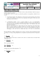
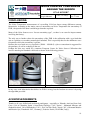
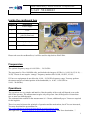
1
NOISE SOURCES COMPARITION AROUND THE EUROPE Sergio Mariotti RAPPORTO INTERNO IRA N° 439 / 2010 Noise source calibration with a travelling amplifier Background: The overall uncertainty in Noise Figure measurements is dominated by the uncertainty in the amount of noise generated by the noise source (Excess Noise Ratio ENR and uncertainty of the ENR). For more than 30 years the most accurate noise generators in the market had an uncertainty +/- 0.12 dB. Leading brands were: Noise/Com , HP/Agilent, Micronetics. In 2003 work between INAF-IRA and Uni. Rome Tor Vergata (UTV) reduced the uncertainty to +/-0.06 dB at frequencies up to 26.5 GHz. A theoretical study between INAF-IRA and UTV showed that the uncertainty cannot be less than 0.055 dB. Note that an uncertainty of the ENR of +/- 0.055dB becomes an uncertainty of §0.09 dB on the noise figure i.e. §7K at ambient temperature. In 2004 Agilent offered a very accurate noise generator ( +/-0.06 dB up to 18 GHz). Comparison of the most accurate noise sources around the Europe: the comparison of the most accurate noise generators cannot further improve the intrinsic accuracy. But a comparison campaign will reveal if each laboratory is inside or outside the uncertainty boundaries. Measurements closer to the overall mean build trust for that particular noise generator and test system. Conversely measurements far from the mean indicate that corrective action (such re-calibration) may be necessary. Organisation of the job: each contributing Institute /Laboratory have performed the measurement of a travelling LNA using their own noise source and related instruments. The measurement has being performed in the most accurate and precise way at room temperature for simplicity in this phase of the test programme. Each Institute has sent the data file to INAF-IRA for the comparison. The project is started in July 2009 and finished in September 2010. PARTNERS INAF-IRA (Italy) CAY (Spain) Uni Canarbia (Spain) Uni. Manchester (U. K.) Astron (Netherlands) Fraunhofer IAF (Germany) others labs in the future? Contact Name S. Mariotti, F. Perini J.D. Gallego, E. Artal , J.L. Cano M. Missous, S. Arshad E. Wan Der Waal H. Massler, B. Aja NOISE SOURCES COMPARISON AROUND THE EUROPE FINAL REPORT Author: Revised by: Date: Sergio Mariotti A. Orfei, J.D. Gallego Oct. 9th 2010 NOISE SOURCES COMPARISON AROUND THE EUROPE FINAL REPORT INTRODUCTION It’s well known that the correct way to furnish an experimental measure is to provide both the observed value and its associated uncertainty. For the low noise amplifiers, the improvement of the technology and the cryogenic cooling has produced a decreasing of the input Noise Temperature down to few times the theoretical quantum limit hQ/k , while the associated uncertainty isn’t affected by any reduction. It isn’t rare a case we quote the noise temperature of an LNA as Te = 10 +/-20 K. The causes that generates and propagates the Uncertainty are well described and discussed in [1] and [2]. Here’s a summary of that causes and typical values for the travelling LNA (described later) measured by a typical mod. 346C Noise Source [3] Uncertainty related to the LNA Noise Figure [strongly dependent on U(ENR)] Uncertainty related to Instrument Noise Figure Uncertainty related to LNA Gain Measurement Uncertainty related to ENR [ dB ] 0.20 0.004 0.01 0.15 Overall (RSS) Uncertainty on Noise Figure (1 V) 0.25 In this case, the NF of the LNA is NF = 1.7 dB +/-0.25 dB or 139 +/-26 K ( 1V). It’s evident that the strongest cause of U(Te) is the U(ENR). The most obvious questions is how the U(ENR) can be reduced? Before to answer, it’s necessary give the answer to another question: What is the minimum theoretical limit of U(ENR) ? The answer may be found in [4] and in [5], and may be summarised as follow: ENR is determined by the help of a radiometric chain. At the input a relays switch sequentially three arms of the chain, the cold standard, the hot standard and the unknown noise source. U(ENR) is the resultant propagation of many causes of uncertainty but the most significant are: The uncertainty of the temperature of the cold noise source U(Tcold) The uncertainty of the spar of the arms of radiometric chain used for comparison U(sij) . 1 NOISE SOURCES COMPARISON AROUND THE EUROPE FINAL REPORT Author: Revised by: Date: Sergio Mariotti A. Orfei, J.D. Gallego Oct. 9th 2010 Given the most accurate data values obtainable from a commercial Network Analyzer and a Standard Cold Load, both operated by a very skilled operator, a Noise Generator may be calibrated with U(ENR) = +/-0.055 dB (1 V) at 18 GHz. For more than 20 years, the most accurate Noise Generators sold by hp/Agilent, the mod. HP346, had U(ENR) quoted +/-0.15 dB (1 V). In the hp/Agilent documents, for the mod. HP346 has been wrote that: the vector method to reduce the U(ENR) was known but not applied [6] the uncertainty was quoted at 1 V instead the more common adopted value 2 V [7]. In Year 2003, a join workgroup of INAF-Institute of Radioastronomy and University of Tor Vergata has lowered the uncertainty of their own Noise Generators by application of the most accurate vector method known [5]. The estimated uncertainty reached was: U(ENR) = +/-0.055 dB (1 V) at 18 GHz. 1 In house Noise Source calibration with secondary standard In year 2004 Agilent started to sell a more accurate Noise Generator, the model series SNS N400x, the related Uncertainty was quoted: U(ENR) = +/-0.06dB (1V) . Despite of the uncertainty has been strongly reduced and the theoretical limit has been almost reached, the value of 0.055 dB cannot be considered a “small” value. Note that realistically, a U(ENR)= 0.055 dB once propagated, produces a U(NF) = 0.09 dB ( +/-7 K at 1 V or +/-14K at 2 V) [3] . What action can be taken in order to further improve the uncertainty? As suggested by [8] and [9] the only possible action is a comparison. The inter-laboratory comparison by itself doesn’t further reduces the uncertainty but it enhances the differences and should suggest some corrective actions, especially for the values farther from the mean. 2 NOISE SOURCES COMPARISON AROUND THE EUROPE FINAL REPORT Author: Revised by: Date: Sergio Mariotti A. Orfei, J.D. Gallego Oct. 9th 2010 COMPARISON The inter-laboratory comparison is not a re-calibration. By itself doesn’t change the ENR of the compared Noise Sources. The differences in readings occurring at each laboratory will not be cleared. Only once this document has been read, each laboratory will have the freedom to apply corrections to ENR. In any case, each correction should be applied with great precaution and cautiousness. The canonical way to do a comparison is a comparison of a travelling standard. An Input Noise Temperature Standard ( an LNA with a standard Noise Temperature) doesn’t exist. Te of LNA is every time dependent on ambient temperature , bias supply and even on the reflection coefficient of the source. But if the travelling LNA will be measured at known ambient temperature, biased by a very stable power supply and close on well matched load , its Te can be considerate stable enough around the travel. The comparison is more accurate as smaller is Te of the LNA. So a cryogenic comparison, in principle, should be preferred to a room temperature comparison [10]. But practically speaking, a balancing of the Pros & Cons must be done: Cryo comparison Man power required Accuracy Sensitivity to how the setup is arranged Sensitivity to U(ENR) Easy to do Probability to find candidate laboratories LNA week (s) ( - ) best ( + ) more ( - ) less ( + ) less ( - ) less ( - ) Room temperature LNA comparison hours ( + ) high (…) less ( + ) more ( - ) more ( + ) more ( + ) Due to that reasons, a room temperature comparison has been preferred. Frequencies: Often the frequency boundaries comes at 18 GHz, 26.5 GHz, 40 GHz, 50 GHz, 67 GHz … The best seller Noise Generators covers the very popular bandwidth 10 MHz-18 GHz. Of course, higher frequencies are also very important for radio astronomy. It has been chosen a frequency range 16…26.5 GHz for the following reasons: x The high end of the bandwidth (say 18 or 26.5GHz) is probably affected by greater uncertainty or errors than the low end of the bandwidth . A comparison is probably more meaningful at the high end of the bandwidth. x 16…26.5GHz has been chosen because step over the 18 GHz boundary. In this way, even the laboratories that are arranged up to 18 GHz may takes advantage of the comparison. 3 NOISE SOURCES COMPARISON AROUND THE EUROPE FINAL REPORT Author: Revised by: Date: Sergio Mariotti A. Orfei, J.D. Gallego Oct. 9th 2010 Reflection coefficient and impedance matching: The LNA has been impedance matched as well as possible, but it cannot be regarded as a well matched device. As higher is the product of the reflection coefficient ( UNS * ULNA) as higher is the ripple of the Te curve over frequency. Two measurements are requested to the laboratories, one placing a selected low VSWR, ferrite circulator in front of the LNA and the other one without that circulator. All the measurements made with the circulator will be compared all together, as well as the measurements performed without the circulator. Comparing the two obtained measurement traces, it’s possible distinguish if the ripple is mainly due to mismatch errors or due to ENR differences. Drift: Since a drift on gain and noise temperature may occur during the measurement session , a measurement of the “thru” is requested both at the beginning and at the ending of the measurement session. If an important drift will be seen , the Te data file will be corrected. Room temperature: The handling of the Noise Source and LNA as well as the solar light coming trough a window, as well as the vicinity of an heater or air conditioning changes the physical temperature of the LNA and consequently it’s Te. For this reason a proper shield form heat/cold sources is required , as well a period of time long enough to reach the thermal equilibrium ( 5 minutes). Aging check: At INAF-IRA the LNA has been measured both at the beginning and one year later at the end of the campaign. Differences on Te was smaller than +/- 2 K except for frequencies greater than 26.3 GHz where the difference was slowly increasing with the frequency up to 10K . 4 NOISE SOURCES COMPARISON AROUND THE EUROPE FINAL REPORT Author: Revised by: Date: Sergio Mariotti A. Orfei, J.D. Gallego Oct. 9th 2010 DATA PROCESSING The data files coming from each one laboratory have been analyzed. Not all data set are organized on the requested way. Some data are 50 MHz spaced while other are 100 MHz spaced. One data set is 500 MHz spaced. This difference has involved a small complication on the processing but does not affects the comparison. Most data set contains Noise Temperature and Insertion Gain while two data set contains NF (dB) only. This small lack does not affect the comparison. Some data set do not include the “initial” and “final” zero traces. It has been assumed that the drift was negligible. Where possible , the drift has been evaluated. For all data set both the Noise and Gain drifts were negligible. Since the data set have been collected at different physical temperatures, a correction has been applied in order to normalize the actual Noise Temperature. The experimental found law 'Te 0.5K / qC has been applied. 'Tamb Two families of Cartesian graphic have been plotted: the case without input isolator (NO_CIRCULATOR) and the case with the isolator in front of the LNA (YES_CIRCULATOR). As it may be seen , the spread is very large. Also it’s difficult to understand the whole traces. A selective analysis is much more indicative. Three kind of analysis has been performed: x The effect of the mismatch loss is analyzed and discussed. x the actual Noise Temperature trace is compared to the mean value (calculated at every frequency along the points coming from each Noise Generator). x Traces performing similar behaviour has been looked for , grouped, analyzed and discussed. What kind of mean? The most known method to estimate the mean value of a number of samples is the calculation of the arithmetic average, accomplished by +/- the standard deviation. An alternative method, widely used at NIST, is the computation of the median accomplished by +/- the MAD [11] . For uniformly and normal distributed samples, the average and median are coincident, as well as the standard deviation and the MAD. But in the case that few samples fall far outside the distribution law, the median better filters away the farther samples. Even the MAD, rather than the standard deviation, better filters the rare and farther samples. So the median method is more robust than the average one. 5 NOISE SOURCES COMPARISON AROUND THE EUROPE FINAL REPORT Author: Revised by: Date: Sergio Mariotti A. Orfei, J.D. Gallego Oct. 9th 2010 RESULTS Impedance Mismatch effects A mismatch error should generates a ripple on the frequency domain representation of the trace. The mismatch error is as large as the trace NO_CIRCULATOR shows more ripple than the trace YES_CIRCULATOR. The mismatch effect has been summarized on the next table: ORGANISATION NOISE GENERATOR Uni Cantabria Uni Cantabria INAF-IRA INAF-IRA Uni Manchester Yebes Yebes Yebes Astron Astron Fraunhofer IAF Fraunhofer IAF HP 346C K01 HP 346C K01+10 dB HP 346C +10 dB HP 346A SNS N4002 HP 346C+10dB NC 346KA+10dB SNS N4002 HP 346A SNS N4000 SNS N4000 SNS N4002 Mismatch error (difference on the ripple) strong absent absent n/a small absent absent small n/a n/a n/a absent Freq. range 16-26.5 16-26.5 16-26.5 16-18 16-26.5 16-26.5 16-26.5 16-26.5 16-18 16-18 16-18 16-26.5 6 NOISE SOURCES COMPARISON AROUND THE EUROPE FINAL REPORT Author: Revised by: Date: Sergio Mariotti A. Orfei, J.D. Gallego Oct. 9th 2010 Charts Noise Temp. of the same LNA measured by different labs. (NO_input_circulator) IRA 346C+10dB IRA 346A U.Cantabria 346CK01 U.Cantabria 346CK01+10dB U. Manchester N4002A Yebes 346C+10dB Yebes 346KA+10dB Yebes SNS N4002 ASTRON 346A ASTRON SNS N4000A Fraunhofer IAF SNS N4002A Fraunhofer IAF SNS N4000A Noise Temperature (Te) [ K ] 240 220 200 180 160 140 120 100 15 17 19 21 23 25 27 Frequency [ GHz ] 2 Noise Temperature of same LNA measured by different labs ( NO_input_circulator) Noise Temp. of the same LNA measured by different labs. (YES_input_circulator) Noise Temperature (Te) [ K ] 280 IRA 346C+10dB IRA 346A U.Cantabria 346CK01 U.Cantabria 346CK01+10dB U. Manchester N4002A Yebes 346C+10dB Yebes 346KA+10dB Yebes SNS N4002 ASTRON 346A ASTRON SNS N4000A Fraunhofer IAF SNS N4002A Fraunhofer IAF SNS N4000A 260 240 220 200 180 160 140 15 17 19 21 23 25 27 Frequency [ GHz ] 3 Noise Temperature of same LNA measured by different labs ( YES_input_circulator) 7 NOISE SOURCES COMPARISON AROUND THE EUROPE FINAL REPORT Author: Revised by: Date: Sergio Mariotti A. Orfei, J.D. Gallego Oct. 9th 2010 Noise Temp. of the same LNA measured by different labs. (YES_input_circulator, 16...18 GHz only) Noise Temperature (Te) [ K ] 280 IRA 346C+10dB IRA 346A U.Cantabria 346CK01 U.Cantabria 346CK01+10dB U. Manchester N4002A Yebes 346C+10dB Yebes 346KA+10dB Yebes SNS N4002 ASTRON 346A ASTRON SNS N4000A Fraunhofer IAF SNS N4002A Fraunhofer IAF SNS N4000A 260 240 220 200 180 160 140 16.0 16.5 17.0 17.5 18.0 Frequency [ GHz ] 4 Noise Temperature of same LNA measured by different labs ( YES_input_circulator, 16...18 GHz only) Even if the different colours may help the trace identification, the whole traces are not the best way to compare different measures because is confusing. A good way to compare each measurement is a plot of every measurement compared with the “mean” of the measurements. As discussed before, the median value, rather the average , better describe the “most probable mean”. 8 NOISE SOURCES COMPARISON AROUND THE EUROPE FINAL REPORT 240 Author: Revised by: Date: Sergio Mariotti A. Orfei, J.D. Gallego Oct. 9th 2010 NO_circ_avg_cor Te YES_circ_avg_cor Te 220 MEDIAN+/-MAD NO_circ_ 200 MEDIAN+/-MAD YES_circ 180 160 140 120 100 16 18 20 22 24 26 24 26 5 INAF-IRA , HP 346C+10 dB attenuator 240 NO_circ_avg_cor Te YES_circ_avg_cor Te 220 MEDIAN+/-MAD NO_circ_ MEDIAN+/-MAD YES_circ 200 180 160 140 120 100 16 18 20 22 6 INAF-IRA , HP346A 9 NOISE SOURCES COMPARISON AROUND THE EUROPE FINAL REPORT 240 Author: Revised by: Date: Sergio Mariotti A. Orfei, J.D. Gallego Oct. 9th 2010 NO_circ_avg_cor Te YES_circ_avg_cor Te 220 MEDIAN+/-MAD NO_circ_ MEDIAN+/-MAD YES_circ 200 180 160 140 120 100 16 18 20 22 24 26 24 26 7 University of Cantabria, HP346CK01 240 NO_circ_avg_cor Te YES_circ_avg_cor Te 220 MEDIAN+/-MAD NO_circ_ MEDIAN+/-MAD YES_circ 200 180 160 140 120 100 16 18 20 22 8 University of Cantabria, HP346CK01+10dB Attenuator 10 NOISE SOURCES COMPARISON AROUND THE EUROPE FINAL REPORT 240 Author: Revised by: Date: Sergio Mariotti A. Orfei, J.D. Gallego Oct. 9th 2010 NO_circ_avg_cor Te YES_circ_avg_cor Te 220 MEDIAN+/-MAD NO_circ_ MEDIAN+/-MAD YES_circ 200 180 160 140 120 100 16 18 20 22 24 26 24 26 9 University of Manchester, SNS N4002A 240 NO_circ_avg_cor Te YES_circ_avg_cor Te 220 MEDIAN+/-MAD NO_circ_ MEDIAN+/-MAD NO_circ_ 200 180 160 140 120 100 16 18 20 22 10 Centro Astronomico de Yebes , HP346C+10dB Attenuator 11 NOISE SOURCES COMPARISON AROUND THE EUROPE FINAL REPORT 240 Author: Revised by: Date: Sergio Mariotti A. Orfei, J.D. Gallego Oct. 9th 2010 NO_circ_avg_cor Te YES_circ_avg Te 220 MEDIAN+/-MAD NO_circ_ MEDIAN+/-MAD YES_circ 200 180 160 140 120 100 16 18 20 22 24 26 24 26 11 Centro Astronomico de Yebes, NC346KA+10dB Attenuator NO_circ_avg_cor Te YES_circ_avg_cor Te 240 MEDIAN+/-MAD NO_circ_ 220 MEDIAN+/-MAD YES_circ 200 180 160 140 120 100 16 18 20 22 12 Centro Astronomico de Yebes, SNS N4002A 12 NOISE SOURCES COMPARISON AROUND THE EUROPE FINAL REPORT 240 Author: Revised by: Date: Sergio Mariotti A. Orfei, J.D. Gallego Oct. 9th 2010 NO_circ_avg_cor Te YES_circ_avg_cor Te 220 MEDIAN+/-MAD NO_circ_ MEDIAN+/-MAD YES_circ 200 180 160 140 120 100 16 18 20 22 24 26 24 26 13 Astron, HP346A 240 NO_circ_avg_cor Te YES_circ_avg_cor Te 220 MEDIAN+/-MAD NO_circ_ MEDIAN+/-MAD YES_circ 200 180 160 140 120 100 16 18 20 22 14 Astron, SNS N4000A 13 NOISE SOURCES COMPARISON AROUND THE EUROPE FINAL REPORT 240 Author: Revised by: Date: Sergio Mariotti A. Orfei, J.D. Gallego Oct. 9th 2010 NO_circ_avg_cor Te YES_circ_avg_cor Te 220 MEDIAN+/-MAD NO_circ_ MEDIAN+/-MAD YES_circ 200 180 160 140 120 100 16 18 20 22 24 26 24 26 15 Fraunhofer IAF, SNS N4002A 240 NO_circ_avg_cor Te YES_circ_avg_cor Te 220 MEDIAN+/-MAD NO_circ_ MEDIAN+/-MAD YES_circ 200 180 160 140 120 100 16 18 20 22 16 Fraunhofer IAF, SNS N4000 14 NOISE SOURCES COMPARISON AROUND THE EUROPE FINAL REPORT Author: Revised by: Date: Sergio Mariotti A. Orfei, J.D. Gallego Oct. 9th 2010 Trace behaviour, similarities and noise generators summary In the following table the behaviour of the compared noise generators and the uncertainty labelled by the factory are summarized ORGANISATION Uni Cantabria Uni Cantabria INAF-IRA INAF-IRA Uni Manchester Yebes Yebes Yebes Astron Astron Fraunhofer IAF Fraunhofer IAF INAF-IRA INAF-IRA NOISE GENERATOR HP 346C K01 (1) HP 346C K01+10dB HP 346C +10 dB HP 346A SNS N4002 HP 346C+10dB NC 346KA+10dB (3) SNS N4002 HP 346A SNS N4000 SNS N4000 SNS N4002 HP 346C +10 dB HP 346 Date 20/07/2009 20/07/2009 03/09/2009 17/08/2009 30/10/2009 30/11/2009 30/11/2009 30/11/2009 20/04/2010 20/04/2010 25/05/2010 25/05/2010 08/06/2010 08/06/2010 Freq. range 16-26.5 16-26.5 16-26.5 16-18 16-26.5 16-26.5 16-26.5 16-26.5 16-18 16-18 16-18 16-26.5 16-26.5 16-18 Similar behaviour Uncertainty u(ENR) +/- 0.12 +/- 0.12 Ŷ CM +/- 0.06 (2) Ŷ CM +/- 0.12 +/- 0.06 ż +/- 0.12 Ŷ CM +/- 0.12 +/- 0.06 ż CM +/- 0.12 +/- 0.06 CM +/- 0.06 +/- 0.06 ż Repeatibility check Repeatibility check Where: (1) (2) (3) Ŷ ż CM K01 stands for 1GHz…50GHz 2.4mm coax connector. Uncertainty reduced by in-house calibration KA stands for 10MHz…40GHz 2.92mm coax connector. the behaviour of the traces is similar among themselves the behaviour of the traces is similar among themselves the trace is closer to median value It has been looked for the most similar curves. In the following two graphics are plotted le closest curves because the number of similar families of curves is two. 15 NOISE SOURCES COMPARISON AROUND THE EUROPE FINAL REPORT Author: Revised by: Date: Sergio Mariotti A. Orfei, J.D. Gallego Oct. 9th 2010 As it may be seen in the following charts, the measurements performed by laboratories that involves the mod. NC346C + 10 dB attenuator are closer among themselves. Also measurements performed by laboratories that involves the SNS N4002 are among themselves. But the two families are different among themselves. It may be suspected that the differences may be imputed to differences in the original calibration procedures at Agilent factory. 250 IRA_346C+10dB 240 Uni_Cantabria 346CK01+10dB 230 Yebes_346C+10dB 220 AVG selected over 346C's 210 200 190 180 170 160 150 16 18 20 22 24 26 17 Measurements performed with Noise Generators mod. 346C+10 dB Attenuator by different labs 250 U_Manchester_SNS N4002A 240 Yebes_SNS_N4002A Fraunhofer_IAF_SNS_N4002 230 AVG selected over SNS_N4002A's 220 210 200 190 180 170 160 150 16 18 20 22 24 26 18 Measurements performed with Noise Generators SNS_N4002A by different labs 16 NOISE SOURCES COMPARISON AROUND THE EUROPE FINAL REPORT Author: Revised by: Date: Sergio Mariotti A. Orfei, J.D. Gallego Oct. 9th 2010 ENR TABLE CORRECTION For laboratories like to correct their ENR table in order to reduce the distance from the average or median, a method is described. It’s important to write in an explicit way that this operation is conceptually a mistake for two reasons: x A metrological mistake. The calibration of a Noise Source by the knowledge of Te of LNA is same as the calibration of a pocket rule by comparing to the length of a table desk (while the right way is the contraire). x A mathematical mistake. It isn’t a rigorous method, it’s just s an approximation. The reason is because for a rigorous calculation it should be necessary to know and take into account for the noise temperature of the Noise Figure Meter ( the Calibration data), while those data are unknown. However since the LNA gain is high enough, the Noise Temperature of the Noise Figure Meter is strongly masked, so accepting a small error, the Noise contribution of the noise figure analyzer may be neglected. In any case, even if it’s an approximation the method is converging, so the error will be reduced and there is no risk of overcorrection. But if the difference of ENR is suspected to be very large, a corrective action is perhaps better than do nothing. So, if the preceding simplification is accepted, the actual measured Noise Temperature is: Th Y Tc (1) Y 1 The similar equation form may be written for the value we would read, the corrected Noise Temperature ( T c e ) T c h Y Tc T ce (2) Y 1 Te Now , let perform the ratio, T ce Te Th Y Tc T c h Y Tc (3) Solving for the corrected hot temperature T c h , T ch Th Y Tc Y Tc (4) Te T ce 17 NOISE SOURCES COMPARISON AROUND THE EUROPE FINAL REPORT Author: Revised by: Date: Sergio Mariotti A. Orfei, J.D. Gallego Oct. 9th 2010 Finally the new, corrected ENR value is: ENR c 10 log( T c h To ) To (5) Or , if the operator prefers the advantages of the small correction for Tc z To , even if formally different by the ENR definition, we get: ENR c T c h Tc 10 log( ) 290 (5 bis) Where: Te = Input Noise Temperature of the LNA ( the actual Noise Temperature) Th = Hot Noise Temperature generated by the Noise Generator (the actual value) To = 290 K, The standard temperature Y = The Y factor . T c e = Input Noise Temperature of the LNA ( the wanted value) T c h = Hot Noise Temperature generated by the Noise Generator (the wanted value) ENR = The Excess Noise Ratio (the actual value) ENR c = The Excess Noise Ratio (the wanted value) Note that the variables Te and T c e should not only be considered alone, but also their ratio Te T ce has a physical meaning. The knowledge of the variable Y is required but probably was not recorded at the time of measurement. It doesn’t matter because the Y factor may be calculated offline by solving the (1) for Y and combining the (5) or the (5bis) Th To To 10 Y ENR 10 Te To To 10 Te Tc (6) ENR 10 (7) In order to help users, who want correct their ENR table, a MS Excel file is provided. The user should input, frequency by frequency, the actual ENR, the actual Te and the spreadsheet will calculate the ENR corrected that produce the median Te. 18 NOISE SOURCES COMPARISON AROUND THE EUROPE FINAL REPORT Author: Revised by: Date: Sergio Mariotti A. Orfei, J.D. Gallego Oct. 9th 2010 CONCLUSIONS: The Noise Temperature measurement of a travelling LNA has shown strong differences among laboratories. Assuming as the major cause of uncertainty on Noise Temperature the uncertainty of ENR , the spread of the data is much larger than the expected. Many of the Noise Sources were “lowest uncertainty type”, so there is no room for improvements involving the factory. The only way to further reduce the uncertainty of the ENR is the calibration with a cryo-load that acts as a primary or secondary metrological standard. This is especially thru for the millimetre wave frequencies where the uncertainty is greater. Because the cryo loads are very expensive (50000 – 100000 €) a join or consortium is suggested for the purchase, as well as a sharing in the use. Perhaps the best way would be a common European Centre for Noise Source Calibration that involve metrological standard cold-loads as shown in the following pictures. Noise/Com Cold Load Maury Microwave Cold Load In any case, each laboratories that believe its ENR is wrong, has the freedom to correct it by using the algorithm provided. ACKNOWLEDGEMENTS Thanks to all very skilled and motivated participants , especially to Eduardo Artal and Juan Luis Cano ( Uni of Cantabria, Spain ), Juan Daniel Gallego ( CAY, Spain ) , Mohamed Missous and Shahzad Arshad ( Uni of Manchester, U.K. ), Eric Van Der Waal ( Astron , NL ), Hermann Massler and Beatriz Aja ( Fraunhofer IAF , Germany ), Federico Perini ( INAF-IRA, Italy ). 19 NOISE SOURCES COMPARISON AROUND THE EUROPE FINAL REPORT Author: Revised by: Date: Sergio Mariotti A. Orfei, J.D. Gallego Oct. 9th 2010 BIBLIOGRAPHY [1] N. Kuhn; Curing a Subtle but Significant Cause of Noise Figure Error , Microwave Journal,; June 1984 [2] AN-57-2 , Noise Figure Measurement Accuracy – The Y Factor , hp/Agilent Technologies year 2001 [3] http://contact.tm.agilent.com/data/static/eng/tmo/Notes/interactive/an-NFUCal/uncert.xls [4] W.C. Daywitt; ;Radiometer equation and analysis of systematic errors for the NIST automated radiometers , NIST Technical Note 1327, march 1989 [5] M. De Dominicis; Strumentazione e Metodologie per la Modellistica di Rumore di Dispositivi Attivi ad Alta Frequenza , PhD Thesis Uni. “Tor Vergata” , February 2004 ( in Italian) [6] AN-57-1, Fundamentals of RF and Microwave Noise Figure Measurements , hp/Agilent Technologies , July 1983 [7] Noise Sources 10MHz to 26.5GHz , Hewlett Packard Technical Data , Jan. 1989 [8] http://www.arftg.org/s_parameter_meas.html [9] J. Randa, and others; International Comparison of Thermal Noise-Temperature Measurements at 2, 4, and 12 GHz e , IEEE T.I.M. APRIL 1999 [10] J.D. Gallego, J.L. Cano , Estimation of Uncertainty in Noise Measurements Using Monte Carlo Analysis: , Radionet FP7 Workshop Meeting, June 2009 http://www.radionet-eu.org/fp7wiki/lib/exe/fetch.php?media=na:engineering:ew:gallego_final.pdf [11] http://en.wikipedia.org/wiki/Median_absolute_deviation 20 Inter laboratory Noise Source Comparition User Manual July 2009 Inside the cardboard box Quantity Description 1 Power supply 1 LNA 2 1 Ka Band ferrite circulators with 50 Ohm load. Digital thermometer 1 paper tape 1 This manual Please take care the cardboard box; it will be used for ship back to INAF-IRA. Frequencies The optimal frequency range is 16.00 GHz … 26.50 GHz The steps must be 50 or 100 MHz wide, and includes the integers of GHz (i.e. 16.00, 16.05, 16.10, … 26.50). Please do not acquire “strange” frequency numbers like 16.000, 16.0525, 16.105… If Your own equipments do not allow the 16.00…26.50 GHz frequency range, You may perform the measurement in a limited portion of the bandwidth (i.e. 16.00…18.00 GHz or 18.00…24.00GHz). Operations The operations are very simple and intuitive. But the quality of the result will depend even on the skill of the operator. The measurement require only one person. One skilled person is better than two or more non skilled people. The estimated time needed for the measurement is 1-3 hours, additionally up to 3 hours are required for the logistics. There is no need to known the principle of operation and the motivations, but if You are interested , You may download the presentation on: http://www.radionet-eu.org/fp7wiki/doku.php?id=na:engineering:ew:1stew then right click on Practical aspects on noise figure measurements and “Save destination…”. 1 Inter laboratory Noise Source Comparition User Manual July 2009 The procedure 1. Turn on the Noise Figure Meter (NFM). Set LO power ( if required) and the central frequency (i.e. 22 GHz). Connect the Noise Source and let it chopping (switching ON/OFF quickly). 2. Open the cardboard box, put the power supply, LNA, thermometer and ferrite circulators on the table. Connect LNA to Power Supply, then Power Supply to the mains. The mains must be grounded properly. 3. Wait the warm-up time, typically 30 min for hp8970A/B (mode 1.1), Eaton/Maury, and Agilent NFA If You are using hp8971B (mode 1.5) , at least 2 hours of warm-up are needed. 4. The temperature of environment and the room should be as constant as possible, keep away from direct sunlight, far from air conditioner air flow etc etc. Also, the LNA should be far from the heated air flow coming out from the NFM and or other equipments. 5. Visual check of all coaxial connectors. They must be clean, free or dust, burrs, also check visually the integrity of coaxial cables. Pay attention when connect the circulators, they are expensive devices. Be gently with the connectors. If a circulator drops into the floor or has been mechanically shocked, please write it into the email report. 6. Calibrate the NFM. Use the ferrite circulator S/N 006 as front-end of Your NFM. The calibration plane is now at the input of the ferrite circulator (see Fig. 1). Set an adequate averaging ( not too long time, please!). Wait at least 5 minutes and check the calibration. Redo the calibration once again if far from 0 K. Record the file as initial.* 7. Insert the LNA by gently screwing the K connectors as usual (see Fig. 1). Put the thermometer sensor as close as possible to the end part of the Noise Source body (OUT connector side). Use the paper tape to firmly connect the sensor (see Fig. 2). Paper tape is more thermal isolator than other tapes, also it can be peeled away quickly. note: even in the case You are using an interseries coaxial transition ( i.e. 7mm to SMA or N to SMA) the thermometer sensor should be placed closer as possible to the end part of the Noise Source body. 8. Wait 5 minutes for the thermalizzation. (Your finger has been heated the LNA ! ) 2 Inter laboratory Noise Source Comparition User Manual July 2009 9. If You are using hp8970 or hp8971 or Maury/Eaton NFM : Read the temperature on the digital thermometer, convert in K if necessary, put it into the NFM ( for hp8970 type 6.0 SF) and writes to me by email. If You are using the new Agilent NFA, read both the digital thermometer and the actual Cold Temperature of NFA and writes to me by email both. 10. Perform the measurement (without ferrite circulator at the input of LNA). Record the file as no_circulator.* 11. Disconnect the Noise Source, insert the ferrite circulator s/n 004 (see Fig. 3). 12. wait 5 minutes, check once again the cold temperature, and if necessary set once again into NFA. 13. Perform the measurement (with ferrite circulator at the input of LNA). Record the file as circulator.* 14. disconnect the LNA and connect the Noise Source to NFM. 15. Wait 5 minutes and perform the 4th and last measurement. This is a 0K check in order to know the drift during the procedure. Record the file as final.* 16. The measurement is finished. Put the LNA, ferrite circulators and all the materials into the cardboard box , and ship back . 17. Send an email to [email protected] containing the following: 1 - The four text files. 2 - The value of Cold Temperature. 3 - Type of conversion (SSB or DSB ?) 4 - A brief description of the setup including the equipment p/n. 5 - Name and contact of the person that really have made the measurement. 6 - The tracking number of the shipment. 7 - Some additional in formations if necessary or needed. Fig. 1 Screwing the coax connector Fig. 2 The thermometer sensor is installed 3 Inter laboratory Noise Source Comparition User Manual July 2009 Fig. 3 The ferrite circulator in front of the LNA Expected Results Once all partner will have performed the measurements, the data will be collected and plotted together on the same graphic, The plot will be sent to all partners. Postal address: Mr. Sergio Mariotti INAF-IRA Radiotelescopio di Medicina v. Fiorentina 3508/B I – 40059 MEDICINA (BO) ITALY Email: [email protected] INAF - Ist. di Radioastronomia www.ira.inaf.it Phone +39 051 6399356 , +39 051 6965829 Mobile +39 328 6248631 , Fax +39 051 6965810 4