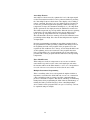
1
Remote Programming
for the Agilent 86140 series
of Optical Spectrum
Analyzers
Product Note 86140-1
Introduction
This programming guide is provided as an introduction to remote
programming of the Agilent 86140-series optical spectrum analyzers
using a personal computer or workstation. While this guide shows
examples written in HP-BASIC, virtually any language may be used in
remotely programming the OSA. The main purpose of this product note
is to demonstrate OSA programming concepts and common remote
tasks. Of secondary importance will be explaining the operation of the
General-Purpose Interface Bus, or GPIB.
It is important to become familiar with the operation of the
Agilent 86140 before controlling it over the GPIB. A good knowledge
of OSA control from the front panel will facilitate the development of
efficient programs to control the analyzer remotely.
The experienced instrument programmer may want to read only the
sections called “Multiple Instrument Programming” (page 10), Common
Remote Commands (page 12) and Programming Examples (page
14). He or she most likely will be familiar with all other topics of this
document.
While this programming guide discusses the General-Purpose Interface
Bus, and shows programming examples in HP-BASIC, it is not a
detailed manual for either topic. Questions related to these topics
can be addressed by referring to their respective manuals. Helpful
documents containing more information on GPIB, HP BASIC, and
the OSA are listed below.
Info on the Agilent 86140 series of OSAs
Agilent 86140 User’s Guide
86140-90001
Info on GPIB operation
Consult your GPIB card manual
Info on HP BASIC for Windows
User’s Manual
Reference Manual
2
E2060-90001
E2060-90002
Table of Contents
Required Equipment .......................................................................................4
System Setup ...................................................................................................4
System Operation............................................................................................6
Remote Programming Advantages ...............................................................8
OSA Programming Concepts.........................................................................8
Frequently Used Remote Commands.........................................................12
Programming Examples...............................................................................16
• Example 1: Simple Measurement ............................................................16
• Example 2: Passband Measurement........................................................18
• Example 3: Signal Monitoring ..................................................................20
3
Required Equipment
Three pieces of equipment are required to remotely control the optical
spectrum analyzer:
1. An Agilent 86140-series optical spectrum analyzer.
2. A personal computer or workstation equipped with a general purpose
interface bus (GPIB) card (also known as an IEEE-488 interface bus
card) and enough memory to store the programming language and
any programs developed.
3. An Agilent 10833A/B/C/D GPIB cable to connect the computer to
the OSA.
To follow the examples in this product note, a copy of HP BASIC is
also needed.
Other Useful Equipment
1. A source (DFB laser, LED, Erbium ASE source, tunable laser, etc.)
2. Fiber jumpers, patch cords, optic cables
3. A device under test (DUT)
System Setup
1. Connect the OSA and computer using a GPIB cable as shown in
Figure 3. The cable connection on the OSA is located on the rear panel
of the instrument. Refer to the Figures 1 and 2 below for the exact
location. The cable connection on the computer is located where the
GPIB card resides, most likely on the back of the computer.
Figure 1. Rear panel of benchtop OSA
4
Figure 2. Rear panel of portable OSA
GPIB Cable
Figure 3: GPIB Connection
2. Turn on the OSA and set its device address by first pressing the
“System” key located below the display. Next press the softkey “More
System Functions& “ and then the softkey “Remote Setup... “. This will
bring up a panel entitled Remote Setup as shown in Figure 4. This
panel allows the OSA address to be selected. The default address is 23.
This can be changed by entering the desired address and pressing the
“Set GPIB Address” softkey. Examples in this product note use the
default address.
5
Figure 4. Remote Setup panel
3. Check the settings of the GPIB card and verify its operation. To do
this, consult the particular GPIB (IEEE-488) manual. Generally no
modifications will need to be done to the card.
4. Turn on the computer and open the programming environment. Each
language handles output devices differently, so it will be necessary to
understand the section in the programming manual that deals with
output devices. In the case of HP BASIC, output devices use the
command string:
OUTPUT <address>; “<SCPI command>”
For example, to send the “Reset” command remotely, the syntax in
HP BASIC is:
OUTPUT 723; “*Rst”
The HP BASIC “OUTPUT” command goes to address 7 on the GPIB
card and sends the command string to the device at address 23. It
is very important to note that in HP BASIC “OUTPUT” has an implicit
linefeed character at the end of the line. If another programming
environment is used, this linefeed character may need to be added.
In most cases this will require adding a “\n” at the end of the SCPI
command.
System Operation
To remotely control the optical spectrum analyzer, the computer sends
commands over the GPIB cable. Once the OSA receives a command, it
goes into “remote” operation and executes the command sent. Remote
operation of the OSA is indicated by the illumination of the yellow “RMT”
LED located on the top middle portion of the instrument, and red
“RMT” text on the upper right-hand corner of the display screen (See
Figure 5). Once the OSA is in remote mode, commands entered by
pressing buttons on the front panel of the instrument WILL NOT be
executed. To return control back to the front panel press the “Local”
button next to the RMT LED.
6
Remote Text “RMT”
Remote LED
“Local” Button
Figure 5. Remote Indicators
The GPIB interface is a simple connection between the PC and the
instrument (an OSA in this case). It allows one command to be
sent at a time. For this reason, all commands sent during remote
operation are executed sequentially. For the Agilent 86140, the
execution of a command will not begin until the previous command
has finished its execution. As a result, there are no timing issues
in remote programming of the 86140 series of optical spectrum
analyzers. This is very important to note, as many other test and
measurement devices work differently and timing may be an issue.
Commands for the 86140 series conform to the Standard Commands
for Programmable Instruments (SCPI) standard. The commands are
derived from SCPI version 1997.0. Some commands do exist which are
not covered by the 1997.0 standard. In this case new SCPI commands
have been defined which have the same form and feel as the 1997.0
commands.
7
Remote Programming
Advantages
Remote programming offers multiple advantages. One advantage is
speed. Repetitive measurements can be made much more quickly when
running a remote program to control the state of the OSA as opposed
to locally controlling it (pushing front panel buttons to make the
measurement). In many cases, one SCPI command is equivalent to
multiple keystrokes on the front panel.
Repeatability is another advantage. It insures that exactly the same
measurement is performed each time the program is run. This enables
comparisons of data from different program runs to be made.
Another advantage to remote programming is the ability to query
information from the OSA and store it in a file on a computer.
Comprehensive records of all measurements made may be created.
Speed and storage capacity gained from remote programming results in
a huge advantage: automation. With remote programming, one can totally
automate measurements, essentially creating their own applications.
OSA Programming
Concepts
The most important task in remote programming, especially for
beginning OSA programmers, is to perform the measurement locally
step by step. Record each keystroke, and then translate the
keystroke(s) into its equivalent SCPI command or set of SCPI
commands. Note that this translation may not necessarily have a one
to one correspondence. As the programmer becomes more familiar
with the OSA and how it functions, this step will have less importance.
The first step to take in a remote program is to put the instrument
in a known state. This is typically accomplished using the “*RST”
SCPI command. If the programmer does not know the state that the
instrument is in before they start sending commands, they may make
a mistake in their measurement. Functions of the OSA work differently
depending upon its previous state. For example, if “peak search” was
performed while the OSA displayed wavelengths from 1540 nm to
1560 nm, and the peak signal desired was at 1535 nm, the marker
would not find that peak. “Peak search” only searches the wavelength
range shown on the OSA’s display.
8
Typically any measurements done through remote programming should
be accomplished using single sweeps. The OSA is set to not continually
sweep, and only sweeps when sent a “single sweep” command. “*RST”
is typically used at the beginning of most remote programs to reset
the OSA and perform one sweep over the entire wavelength range.
Generally, in analyzing a signal, set up the desired parameters
(wavelength range, sensitivity, resolution bandwidth, etc.), initiate a
single sweep, and then perform the desired measurements on the trace.
Once a measurement has been made, the OSA can be queried to obtain
any desired information. This information can be stored in a variable in
the program and as data in a file. Many times the queried information
will be used by a remote program to set up the state of the OSA for
subsequent measurements. Queried information can include anything
from marker values and data point values to the sensitivity and
resolution bandwidth settings.
Simply put, the more familiar the programmer is with the OSA, the
more efficient they will become in writing remote programs. Efficient
OSA programs revolve around knowing the state the OSA will be in
before executing a command.
In summary, the following is a typical three-step process that should
be followed in most cases when performing a measurement through
remote programming.
1. Put the OSA in a known state. At the beginning of the program, this
will most likely begin with the “Reset” command followed by other
commands to set up the state (i.e., resolution bandwidth, sensitivity,
etc.). At any other point in a remote program, the state of the OSA
will have been determined by previous commands, and thus will
already be in a known state.
2. Take a single sweep to display the signal under the state set up by
previous commands.
3. Perform the desired measurements (i.e., –3dB bandwidth, peak
amplitude, peak wavelength, etc.). This step also includes any
querying* of the OSA.
* Note that whenever wavelength information is queried the value returned is in meters.
9
Auto-Align Feature
Auto-align is a function used to optimize the level of the input signal
for best measurement results. It can be performed either by pressing
the “Auto-Align” button at the bottom of the display, or by sending a
remote command. In general, once auto-align has been performed, it
need not be performed again until operating conditions change (i.e.
temperature changes, the instrument is bumped, etc.). It is important
NOT to perform an auto-align just after the OSA has been turned on.
The OSA’s temperature at power-up will be different from its operating
temperature. An auto-align performed at power-up will be based
upon “power-up” temperature instead of operating temperature.
The OSA should be allowed to warm-up for at least 30 minutes before
performing an Auto-Align. Note that the Auto-Align function requires
an input signal.
In remote programming, performing an auto-align is required only if
the programmer feels that operating conditions will change between
the beginning and end of the program. If the program is to be run
repetitively and conditions are to change, an auto-align should be run
at the beginning, and every n iterations of the program thereafter.
It is very important to be careful and make sure an auto-align is not
performed in a remote program until the OSA has reached operating
temperature.
Trace Math Feature
When using trace math, it is important to use two traces with the
same number of points over the same wavelength span, otherwise
the function will not work. There must be a one to one correspondence
for each of the two traces that are involved in the trace math.
Multiple Instrument Programming
When controlling other devices along with the Agilent 86140 it is
important to remember the 86140 will only execute one command at
a time and will not start execution of another command until the
previous command is complete. This has the advantage of eliminating
timing issues when programming the OSA. It has the disadvantage of
making the OSA a potential “bus hog” when controlling multiple
devices with a remote program. This concept of a “bus hog” can best
be explained using an example.
10
When controlling an OSA and TLS (tunable laser source) with a
remote program, the states of the OSA and TLS are set, and then the
following commands are executed:
Output Osa; “Init:Imm”
Output Osa; “Calc:Mark1:Func:Bwid:Stat On”
Output Osa; “Calc:Mark1:Func:Bwid:Ndb -3 dB”
Output Tls; “<Tls command 1>”
Output Tls; “<Tls command 2>”
Output Tls; “<Tls command 3>”
Output Tls; “<Tls command 4>”
These commands will:
Take a single sweep
Turn on the bandwidth markers
Set the bandwidth markers to -3 dB
Perform 4 different TLS commands
Suppose the OSA sweep in the first command will take many
seconds. The computer will put the first command on the bus and
the OSA will begin executing it. The computer will then put the second
command on the bus. The OSA, however, cannot begin execution of this
command until it has finished execution of the first command (i.e. the
single sweep). This results in the second command sitting on the bus,
preventing any further commands from being sent over it. The bus is
held until the sweep is finished and the OSA can accept the second
and third commands. Once the OSA commands are finished, the TLS
commands will be executed.
If the TLS commands to execute in the above example do not depend
on the information gained from the bandwidth measurements of the
OSA, then a better command order would be:
Output Osa; “Init:Imm”
Output Tls; “<Tls command 1>”
Output Tls; “<Tls command 2>”
Output Tls; “<Tls command 3>”
Output Tls; “<Tls command 4>”
Output Osa; “Calc:Mark1:Func:Bwid:Stat On”
Output Osa; “Calc:Mark1:Func:Bwid:Ndb –3 dB”
11
The computer would send the first command over the bus, as before,
and the OSA would begin execution of it. The second command is
now addressed to the TLS. The computer will then put this second
command on the bus and the TLS will begin execution of it. It will
continue with the other TLS commands and then come to the bandwidth
commands for the OSA. In this second example, the TLS is executing all
its commands while the OSA is sweeping. In the first example the TLS
could not perform any of its commands until the OSA had finished it’s
sweep. The result of the second example is a faster processing time.
In summary, if a command is sent to the Agilent 86140 which will take
some time and another device is being controlled, send the next
commands to the other device to execute while the OSA is executing
its command.
A note to the experienced programmer...
For those who have programmed test and measurement devices
before, some form of “operation complete” query in the program code
may have been used. This was done to insure correct timing in the
execution of remote commands. It is also good programming practice.
As the Agilent 86140 will not execute a command until it is finished
with the previous command, there is no timing issue. The “operation
complete” query need not be used as frequently, or at all.
Frequently Used Remote
Commands
The following is a list of common remote commands. Note that the
actual SCPI command, which will be used with all programming
languages, is the string enclosed in quotes. Also note that Osa is
equivalent to 723. This assignment is accomplished in HP BASIC with
the following line of code:
Osa = 723
Perform an Auto Measure
OUTPUT Osa;”Disp:Wind:Trac:All:Scal:Auto”
Perform an Auto-Align
OUTPUT Osa;”Cal:Alig:Auto”
Perform an instrument reset
OUTPUT Osa;”*Rst”
Perform an instrument preset
OUTPUT Osa;”Syst:Pres”
12
Set start and stop wavelength
OUTPUT Osa;”Sens:Wav:Star 1150 nm”
OUTPUT Osa;”Sens:Wav:Stop 1700 nm”
Set wavelength span
OUTPUT Osa;”Sens:Wav:Span 1100 nm”
Set sensitivity
OUTPUT Osa;”Sens:Pow:Dc:Rang:Low –60 dBm”
Set resolution bandwidth
OUTPUT Osa;”Sens:Bwid:Res 10 nm”
Set reference level
OUTPUT Osa;”Disp:Wind:Trac:Y:Scal:Rlev 0 dBm”
Set vertical scale
OUTPUT Osa;”Disp:Wind:Trac:Y:Scal:Pdiv 10 dB”
Turn on bandwidth markers and set to –3dB
OUTPUT Osa;”Calc:Mark1:Func:Bwid:Stat On”
OUTPUT Osa;”Calc:Mark1:Func:Bwid:Ndb –3 dB”
Query the bandwidth value and center wavelength value
OUTPUT Osa;”Calc:Mark1:Func:Bwid:Res?”
ENTER Osa;Bndwdth
OUTPUT Osa;”Calc:Mark1:Func:Bwid:X:Cent?”
ENTER Osa;Cntrwl
Note: the above set of query commands queries the instrument for
the bandwidth value and the center wavelength value as determined
by the bandwidth function. The bandwidth value is placed in the
variable “Bndwdth” and the center wavelength value is placed in the
variable “Cntrwl”.
Query the marker value
OUTPUT Osa;”Calc:Mark1:X?”
ENTER Osa;MkrWl
OUTPUT Osa;”Calc:Mark1:Y?”
ENTER Osa;MkrAmp
Note: the above set of query commands queries the instrument
for the wavelength value of the marker, puts it in a variable called
“MkrWl”, queries the instrument for the amplitude value of the marker,
and then puts this value in a variable called “MkrAmp”.
13
Query amplitude information of trace
OUTPUT Osa;”Trac:Data:Y? TrA”
ENTER Osa;Ydata(*)
Note: the above commands query the instrument for the amplitude
information of Trace A and stores it in an array with the same
dimensions as the number of trace data points
Display a trace and continuously update
OUTPUT Osa;”Disp:Wind:Trac:Stat TrA, On”
OUTPUT Osa;”Trac:Feed:Cont TrA, Alw”
Freeze data in a trace
OUTPUT Osa;”Trac:Feed:Cont TrA, Nev”
Trace Max or Min hold (Trace A)
OUTPUT Osa;”Calc1:Max:Stat On”
or
OUTPUT Osa;”Calc1:Min:Stat On”
Note: for any command in the “Calc” menu, the number corresponds to
the trace being affected. For example, “Calc1” affects trace A while
“Calc2” affects trace B.
Trace averaging
OUTPUT Osa;”Calc1:Aver:Stat On”
OUTPUT Osa;”Calc1:Aver:Coun 50”
Trace math (C=ALOG-B)
OUTPUT Osa;”Calc1:Math:Expr (TrA / TrB)”
OUTPUT Osa;”Calc1:Math:Stat On”
Set display to linear mode
OUTPUT Osa;”Disp:Wind:Trac:Y:Scal:Lin On”
14
Plug & Play Drivers
Today the most popular form of remote programming is done with
graphical programming languages such as HP VEE and National
Instrument’s LabVIEW. Graphical languages facilitate the development
of programs, making them easier to write and easier to understand.
To further aid graphical programming many instruments are provided
with what are known as Plug & Play drivers. These drivers are
designed for each particular graphical programming language and
provide higher level commands. Basically Plug & Play drivers are
software that consists of a structured list of commands that can be
sent to the instrument to perform an operation.
The Agilent 86140 Series of Optical Spectrum Analyzers come standard
with Plug & Play drivers. Because these drivers are based upon using
dynamic link libraries, they can be used with HP VEE, LabVIEW,
LabWindows, Visual C and any other programming language that
can make use of dynamic link libraries. These drivers consist of
many commands that are analogous to the SCPI commands described
earlier. One of the big advantages to Plug & Play drivers is that
programming becomes a matter of “pointing and clicking” on desired
commands instead of laboriously typing out command strings.
For more information on how to use Plug & Play Drivers, consult
either an HP VEE manual or a LabVIEW manual.
Drivers for the Agilent 86140-series of optical spectrum analyzers can
be found at the website.
15
Programming
Examples
Example 1: Setting the OSA state and querying the OSA
Suggested equipment: Laser source between 1290 nm and 1310 nm
This example demonstrates how to do a simple measurement. Note that after the “Reset” command is
given in line 120, lines 140 through 170 are then used to set up the desired state of the OSA. A sweep is
then taken (line 190) followed by some more OSA setup. One more sweep is taken followed by the desired
measurements.
10 ! Program: Simple HP BASIC Example
20 !
30 !
40 !
50 ! This program sets a start and stop wavelength, finds the largest
60 ! signal within that wavelength span, zooms in, and then finds the -3dB
70 ! bandwidth of the signal.
80 !
90 !
100 !
110 Osa=723
!Make Osa equivalent to 723
120 OUTPUT Osa;”*Rst”
!Perform a OSA Reset to put
130 !
the instrument in known state
140 OUTPUT Osa;”Sens:Wav:Star 1290 nm”
!Set start wavelength
150 OUTPUT Osa;”Sens:Wav:Stop 1310 nm”
!Set stop wavelength
160 OUTPUT Osa;”Sens:Pow:Dc:Rang:Low -60 dBm”
!Set sensitivity
170 OUTPUT Osa;”Sens:Bwid:Res .1 nm”
!Set resolution bandwidth
180 !
190 OUTPUT Osa;”Init:Imm”
!Take a single sweep
The above lines of code are used to set up the OSA to display the wavelength versus power trace from
1290 nm to 1310 nm. The sensitivity and resolution bandwidth are set to maximize the measurement
of power in this range. Notice the procedure of first setting up the state of the OSA followed by taking
a sweep.
200 OUTPUT Osa;”Calc:Mark1:Max”
210 OUTPUT Osa;”Calc:Mark1:Scen”
220 OUTPUT Osa;”Calc:Mark1:Srl”
230 OUTPUT Osa;”Init:Imm”
!Do a peak search
!Marker to center
!Marker to reference level
Lines 200 through 230 are used to find the peak power in the range displayed, move that peak to the
center of the display, and set the reference level of the display to the peak power
16
240 OUTPUT Osa;”Calc:Mark1:X?”
250 !
260 ENTER Osa;Pkwl
270 OUTPUT Osa;”Calc:Mark1:Y?”
280 !
290 ENTER Osa;Pkamp
300 OUTPUT Osa;”Calc:Mark1:Func:Bwid:Stat On”
310 OUTPUT Osa;”Calc:Mark1:Func:Bwid:Ndb -3 dB”
320 OUTPUT Osa;”Calc:Mark1:Func:Bwid:Res?”
330 ENTER Osa;Bw
340 !
350 PRINT “Peak wavelength is: “;Pkwl*1.E+9;” nm”
360 PRINT “Peak amplitude is: “;Pkamp;” dBm”
370 PRINT “Bandwidth (-3dB): “;Bw*1.E+9;” nm”
380 !
390 END
!Query OSA for wavelength value
of marker
!Store wavelength value in variable
!Query OSA for amplitude value
of marker
!Store amplitude value in variable
!Turn on bandwidth marker function
!Make bandwidth display –3dB
!Query OSA for bandwidth value
!Store bandwidth value in variable
!Print peak wavelength in nm
!Print peak amplitude
!Print -3dB bandwidth
Commands in lines 240 through 390 query information from the OSA and then display it on the screen.
This is the final step in the process: making the measurements (in this case the –3 dB bandwidth)
and querying the OSA for the desired data.
17
Example 2: Passband Device Measurement
Suggested equipment: Broadband source around 1550 nm and passband filter between
1535 nm and 1635 nm
This example shows how one may create a remote program to determine the wavelength versus loss
trace of a passband filter and find its -3 dB bandwidth.
10 ! Program: Passband Measurement
20 !
30 ! This program determines the –3 dB bandwidth of a passband filter,
40 ! and displays it’s wavelength versus loss trace.
50 !
60 !
70 Osa = 723
!Make Osa equivalent to 723
80 OUTPUT Osa;”*Rst”
!Put Osa in known state
90 CLEAR SCREEN
100 PRINT “ “
!Print blank line
110 PRINT “Please connect broadband source to Osa in order to take
120 PRINT “a reference level measurement”
130 INPUT “Please press ‘c’ to continue”,Ans$
140 IF Ans$=”C” OR Ans$=”c” THEN
150 GOTO 190
160 ELSE
170 GOTO 130
180 END IF
190 !
200 !*****************Reference Level Measurements************************
210 !
220 OUTPUT Osa;”Sens:Wav:Star 1535 nm”
!Set start wavelength
230 OUTPUT Osa;”Sens:Wav:Stop 1635 nm”
!Set stop wavelength
240 OUTPUT Osa;”Sens:Pow:Dc:Rang:Low –70 dBm”
!Set sensitivity
250 OUTPUT Osa;”Sens:Bwid:Res 0.1 nm”
!Set resolution bandwidth
260 OUTPUT Osa;”Disp:Wind:Trac:Stat TrB, On”
!Turn on trace B
270 OUTPUT Osa;”Trac:Feed:Cont TrB, Alw”
!Continually update trace B
280 OUTPUT Osa;”Init:Imm”
!Single sweep
290 OUTPUT Osa;”Trac:Feed:Cont TrB, Nev”
!Stop updating trace B
295!
The first section of code sets up the state of the OSA and takes a sweep to acquire the reference trace
data. Once the “Init:Imm” command is executed, trace B is “frozen” by remotely sending the “Update Off”
(line 290) command. In this state of “Update Off”, when the passband data is acquired later in the
program the data in trace B, the reference trace, will not be affected.
300 !********************Passband measurements*****************************
305 !
310 OUTPUT Osa;”Disp:Wind:Trac:Stat TrA, On”
!Turn on trace A
320 OUTPUT Osa;”Trac:Feed:Cont TrA, Alw”
!Continually update trace A
330 !
340 !
350 CLEAR SCREEN
18
360 PRINT “Please connect broadband source to input of passband filter”
370 PRINT “and output of filter to input of Osa”
380 INPUT “Please press ‘c’ to continue”,Ans2$
390 IF Ans2$=”C” OR Ans2$=”c” THEN
400 GOTO 440
410 ELSE
420 GOTO 380
430 END IF
440 !
450 OUTPUT Osa;”Disp:Wind:Trac:Stat TrC, On”
!Turn on trace C
460 OUTPUT Osa;”Trac:Feed:Cont TrC, Alw”
!Always update trace C
470 OUTPUT Osa;”Calc3:Math:Expr (A / B)”
!Trace C = Trace A - Trace B
480 OUTPUT Osa;”Calc3:Math:Stat On”
!Math function status “on”
490 OUTPUT Osa;”Init:Imm”
!Take a sweep
Lines 300 through 490 set up the OSA to display the passband data in trace A, and the wavelength
versus loss data in trace C which is derived via the trace math function. Please note that both trace B
and trace A have data over the same wavelength range. This is essential for trace math to work.
500 OUTPUT Osa;”Calc:Mark1:Stat On”
510 OUTPUT Osa;”Calc:Mark1:Trac TrC”
520 OUTPUT Osa;”Calc:Mark1:Max”
530 OUTPUT Osa;”Calc:Mark1:Scen”
540 OUTPUT Osa;”Sens:Wav:Span 10 nm”
550 OUTPUT Osa;”Calc:Mark1:Func:Bwid:Stat On”
560 OUTPUT Osa;”Calc:Mark1:Func:Bwid:Ndb -3 dB”
!Turn on marker
!Put marker on trace C
!Find peak
!Center trace onto marker
!Set span to 10 nm
!Bandwidth marker status “on”
!Bandwidth –3 dB
Lines 500 through 560 find the max signal in the span (which will be the passband signal), centers
the display at this wavelength, reduces the span (essentially zooming in), and turns on the bandwidth
marker to -3dB
570 OUTPUT Osa;”Calc:Mark1:Func:Bwid:Res?”
580 ENTER Osa;Banwdth
590 OUTPUT Osa;”Calc:Mark1:Func:Bwid:X:Cent?”
600 ENTER Osa;Center
610 CLEAR SCREEN
620 PRINT “Bandwidth (–3dB): “;Banwdth*1.E+9;” nm”
630 PRINT “Center Wavelength: “;Center;” nm”
640 END
!Query for bandwidth
!Enter bandwidth value in “Banwdth”
!Query center wavelength value
!Enter value into “Center”
Lines 570 through 670 query the OSA for the desired data and prints it to the monitor.
19
Example 3: Monitoring a Signal
Suggested equipment: Any source
This program shows how to periodically record trace data from the OSA so as to monitor a signal’s changes.
It is particularly important to notice that in this example the OSA is continuously sweeping as opposed to
using a single sweep. This is done because the program makes use of the max hold and min hold functions.
Note that in a real world application of a program similar to this more data points would be used and the
trace data would most likely be written to a file instead of the monitor.
10 ! Program: Signal Monitoring
20 !
30 !
35 ! This program zooms in on the largest signal and then monitors it
40 ! for 10 minutes, recording trace data every minute and printing it to
50 ! the monitor. Three traces are recorded each time:
60 ! the min trace, the max trace, and the actual trace at the time.
70 !
80 !
90 !
95 DIM Ydata(1:101)
!Set up array for trace data
96 DIM Ymax(1:101)
!Set up array for max trace data
97 DIM Ymin(1:101)
!Set up array for min trace data
98 DIM Wl(1:101)
!Set up array for wavelength trace data
100 !
110 Osa=723
!Make Osa equivalent to 723
120 OUTPUT Osa;”*Rst”
!Perform a system reset
130 OUTPUT Osa;”Disp:Wind:Trac:All:Scal:Auto”
!Perform an Automeasure
135 OUTPUT Osa;”Init:Cont On”
!Put OSA in continuous sweep mode
140 OUTPUT Osa;”Sens:Swe:Poin 101”
!Set trace length to 101 points
150 OUTPUT Osa;”Disp:Wind:Trac:Stat TrB, On”
!Turn on trace B
160 OUTPUT Osa;”Trac:Feed:Cont TrB, Alw”
!Always update trace B
170 OUTPUT Osa;”Disp:Wind:Trac:Stat TrC, On”
!Turn on trace C
180 OUTPUT Osa;”Trac:Feed:Cont TrC, Alw”
!Always update trace C
190 OUTPUT Osa;”Calc2:Max:Stat On”
!Trace B Max hold
200 OUTPUT Osa;”Calc3:Min:Stat On”
!Trace C Min hold
Lines 10 through 200 are used to set up the traces: trace A contains the real time signal while trace B
and trace C contain the max trace values and the min trace values respectively. Note that in this program
the OSA is set to continuous sweep mode. Continuous sweep mode is wanted in this case because the
signals need to constantly be monitored as the max or min value at a certain wavelength could occur at
any time. It is also important to note that a remote “Automeasure” (line 130) puts the OSA in single sweep
mode while an “Automeasure” performed locally will put the instrument in continuous sweep mode.
20
210 OUTPUT Osa;”Sens:Wav:Star?”
220 ENTER Osa;Startwl
230 OUTPUT Osa;”Sens:Wav:Stop?”
240 ENTER Osa;Stopwl
250 OUTPUT Osa;”Sens:Swe:Poin?”
260 ENTER Osa;Tlength
270 Bucket=(Stopwl-Startwl)/(Tlength-1)
280 FOR I=1 TO 101
290 Wl(I)=(Startwl+(Bucket*(I-1)))*1.E+9
300 NEXT I
310 !
!Query for start wavelength
!Query for stop wavelength
!Query for number of data points
!Calculate bucket size
!Calculate wavelength value for each point
The above lines of code are used to calculate the wavelength values at each point of data. Wavelength
values cannot directly be queried, but with the above set of commands, the values can be derived.
315 OUTPUT Osa;”Form Ascii”
!Make trace data into ascii format
320 FOR T=1 TO 10
330 WAIT 60
!Wait one minute
340 OUTPUT Osa;”Trac:Data:Y? TrA”
!Query trace A data
350 ENTER Osa;Ydata(*)
360 OUTPUT Osa;”Trac:Data:Y? TrB”
!Query trace B data
370 ENTER Osa;Ymax(*)
380 OUTPUT Osa;”Trac:Data:Y? TrC”
!Query trace C data
390 ENTER Osa;Ymin(*)
400 PRINT “Time “;T
405 PRINT “Point”,”Wavelength”,”Amp”,”MaxAmp”,”MinAmp”
410 FOR I=1 TO 101
420 PRINT I,Wl(I),Ydata(I),Ymax(I),Ymin(I)
!Print out trace data
430 NEXT I
440 NEXT T
450 END
Lines 315 through 450 are used to read in the trace data and print it out to the monitor. This is done
every minute for ten minutes.
21
For more information about Agilent Technologies
test and measurement products, applications,
services, and for a current sales office listing,
visit our web site,
www.agilent.com/comms/lightwave
You can also contact one of the
following centers and ask for a test and
measurement sales representative.
United States:
Agilent Technologies
Test and Measurement Call Center
P.O. Box 4026
Englewood, CO 80155-4026
(tel) 1 800 452 4844
Canada:
Agilent Technologies Canada Inc.
5150 Spectrum Way
Mississauga, Ontario
L4W 5G1
(tel) 1 877 894 4414
Europe:
Agilent Technologies
Test & Measurement
European Marketing Organization
P.O. Box 999
1180 AZ Amstelveen
The Netherlands
(tel) (31 20) 547 2000
Japan:
Agilent Technologies Japan Ltd.
Call Center
9-1, Takakura-Cho, Hachioji-Shi,
Tokyo 192-8510, Japan
(tel) (81) 426 56 7832
(fax) (81) 426 56 7840
Latin America:
Agilent Technologies
Latin American Region Headquarters
5200 Blue Lagoon Drive, Suite #950
Miami, Florida 33126, U.S.A.
(tel) (305) 267 4245
(fax) (305) 267 4286
Australia/New Zealand:
Agilent Technologies Australia Pty Ltd
347 Burwood Highway
Forest Hill, Victoria 3131, Australia
(tel) 1-800 629 485 (Australia)
(fax) (61 3) 9272 0749
(tel) 0 800 738 378 (New Zealand)
(fax) (64 4) 802 6881
Asia Pacific:
Agilent Technologies
24/F, Cityplaza One, 1111 King’s Road,
Taikoo Shing, Hong Kong
(tel) (852) 3197 7777
(fax) (852) 2506 9284
Technical data subject to change
Copyright © 1996, 2000
Agilent Technologies
Printed in U.S.A. 9/00
5968-1548E