Download Hall A Tech Notes JLAB-TN-02-012

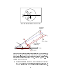
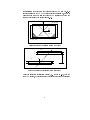
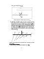
JLAB-TN-02-012
Optics Calibration of the Hall A High
Resolution Spectrometers using the new
optimizer
Nilanga Liyanage
[email protected]
July 18, 2002
1 Introduction
Most up-to-date version of this document can be found at
http://www.jlab.org/~nilanga/physics/optics.ps
The Hall A High Resolution Spectrometers are an identical pair of QQDQ
magnetic spectrometers with optical properties that are point-to-point in the
dispersive direction. The optics matrix elements allow for the reconstruction of
the interaction vertex in the target from the coordinates of the detected particles
at the focal plane. This document describes the optics calibration procedure
used to determine the optics matrix elements. The rst part of this document
describes the basics of optics optimization. The second part of the document
describes the testing procedure of the available data bases while the last part is
a step-by-step user manual for the newly written optimize optimization routine.
The input data for optimize is supplied by The Hall A event analyzer ESPACE.
This manual assumes that the user has a good working knowledge of ESPACE.
Optics matrix elements for both spectrometers have been optimized over the
full ranges both spectrometers1. This optimization has been performed for the
normal tune of the HRS pair. The spectrometer tune, and hence spectrometer
optics, is very sensitive to the ratio of the magnetic eld in the Dipole to the
magnetic elds in the second and the third quadrupoles (Q2 and Q3) . In order
to ensure that normal tune of the
spectrometer, Q2 and Q3 have to be cycled
using the prescribed procedure2. The matrix elements have been tested with
data obtained over one year and have been shown to be stable to the accuracy
1 Nominal momentum ranges are: Right HRS: 0.4 GeV-3.0 GeV; Left HRS 0.4 GeV-4.0
GeV
2 When the spectrometer momentum has to be increased, rst raise Q2 and Q3 currents to
the highest allowed values for that spectrometer (1400 Amp. for Right HRS, and 1600 Amp
for Left HRS) and then go down to the desired momentum. Note that Dipoles should not
be cycled
1
quoted in section 3.0.1. Contact Doug Higinbotham at dougjlab.org to obtain
these matrix elements.
While the optics matrix elements already available will work all the experiments within the nominal ranges of the spectrometers, the focal plane detector
parameters and the osets between the actual detector coordinates and the the
ideal spectrometer coordinates can change from time to time. Therefore before the available databases are used for the analysis of an experiments, these
databases have to be tested for data taken during that experiment. The testing
procedure is described in section 2.
2 Coordinate systems
A detailed description of the coordinate systems used in this document is given in
reference [1]. For convenience, a short overview is presented here. All coordinate
systems presented are Cartesian. Note that a reference to an angular coordinate
in this section should be taken to refer to the tangent of the angle in question.
Hall Coordinate System (HCS): The origin of the HCS is at the center
of the hall, which is dened by the intersection of the electron beam and
the vertical symmetry axis of the target system. z^ is along the beam line
and points in the direction of the beam dump, and y^ is vertically up. See
Fig. 1.
Target Coordinate System (TCS): Each of the two spectrometers
has its own TCS. A line perpendicular to the sieve slit surface of the
spectrometer and going through the midpoint of the central sieve slit hole
denes the z axis of the TCS for a given spectrometer. z^tg points away
from the target. In the ideal case where the spectrometer is pointing
directly at the hall center and the sieve slit is perfectly centered on the
spectrometer, the ztg axis passes through the hall center. For this case,
the distance from the hall center to the midpoint of the central sieve slit
hole is dened to be the constant Z0 for the spectrometer3. The origin of
the TCS is dened to be the point on the ztg axis at a distance Z0 from
the sieve surface. In the ideal case, the origin of the TCS coincides with
the hall center. The xtg axis is parallel to the sieve slit surface with x^tg
pointing vertically down. The out-of-plane angle (tg ) and the in-plane
angle (tg ) are given by dxZ0tg and dyZtg0 respectively. See Fig. 2.
3 Z0HRSE = 1:181 m, Z0HRSH = 1:178 m.
2
HR
SH
Y
Z
HR
SE
Beam
dump
X
Figure 1: Hall Coordinate System (top view)
Scattered
electron
y
sieve
ytg
φ tg
L
y
tg
D
Θ0
z
z tg
Sieve plane
Spectrometer
central ray
Beam
react
Hall center
Figure 2: Target coordinates for electrons scattering from a thin foil target, as
seen from above. L is the distance from Hall center to the sieve plane, while D
is the horizontal displacement of the spectrometer axis from its ideal position.
Spectrometer central angle is denoted by 0. Note that xtg and xsieve are
vertically down (into the page)
The intersection of wire 184 of
the VDC1 U1 plane and the perpendicular projection of wire 184 in the
VDC1 V1 plane onto the VDC1 U1 plane denes the origin of the DCS.
Detector Coordinate System (DCS):
3
^ is parallel to the short symmetry axis of the lower VDC (see Fig. 3). z^
is perpendicular to the VDC1 U1 plane pointing vertically up, and x^ is
along the long symmetry axis of the lower VDC pointing away from the
center of curvature of the dipole (see Fig. 4).
y
Y
V1 VDC plane
X
184 (V1)
184 (U1)
U1 VDC plane
Figure 3: Detector Coordinate System (top view)
VDC 2
V2
d1
U2
VDC 1
d2
Z
V1
d1
U1
X
Figure 4: Detector Coordinate System (side view)
Using the trajectory intersection points pvdc;n (where n=1-4), with the
four VDC planes, the coordinates of the detector vertex can be calculated
4
according to
tan 1 = pvdc;3 d
2
pvdc;1
;
tan 2 = pvdc;4 d2 pvdc;2 ;
1
det = p (tan 1 + tan 2 ) ;
2
1
det = p ( tan 1 + tan 2 ) ;
2
1
xdet = p (pvdc;1 + (pvdc;2 d1 tan 2 )) ; and
2
1
0
ydet = p ( pvdc;1 + (pvdc;2 d1 tan 2 ))
2
(1)
(2)
(3)
(4)
(5)
(6)
where the distances d1 and d2 are dened in Fig. 4. These equations may
be derived based on the following assumptions:
{ the VDC sense wires are oriented at 45Æ with respect to the wire
frame.
{ the wires are positioned in planes.
{ the wire planes are parallel to each other and are separated by known
distances.
{ the location of the center of each wire plane is known.
Any deviation from the above assumptions leads to osets in the DCS
coordinates. These osets are corrected when the focal plane vertex is
calculated.
Transport Coordinate System (TRCS) at the focal plane: The
TRCS at the focal plane is generated by rotating the DCS clockwise
around its y-axis by 45Æ. Ideally, the z^ of the TRCS coincides with the
central ray of the spectrometer. However, due to the deviations mentioned
above, the TRCS used by ESPACE can dier from the ideal spectrometer
Transport Coordinate System.
The transport coordinates can be expressed in terms of the detector coordinates by
det + tan 0
tra =
(7)
1 det tan 0
det
(8)
tra =
cos 0 det sin 0
xtra = xdet cos 0 (1 + tra tan 0 )
(9)
ytra = ydet + sin 0 tra xdet
(10)
5
where 0 is the rotation angle, 45Æ.
VDC 2
Z
VDC 1
Y
o
45
U1
X
Figure 5: Transport Coordinate System (side view).
Focal plane Coordinate System (FCS): The focal plane coordinate
system chosen for the HRS analysis is a rotated coordinate system. This
coordinate system is obtained by rotating the DCS around its y-axis by
an angle , where is the angle between the local central ray4 and the z^
axis of the DCS. As a result,
the z^ axis of the FCS rotates as a function of
the relative momentum pp (see Fig. 6). In this rotated coordinate system
the dispersive angle is small for all points across the focal plane. As a
result, the expressions for the reconstructed vertex converge faster during
optics calibrations.
Z det
ρ
Z fp
X fp
Figure 6: The focal plane (rotated) coordinate system as a function of the focal
plane position.
4 The ray with = = 0 for the corresponding relative momentum pp .
6
The transformation to the FCS also includes corrections for the osets
incurred due to misalignments in the VDC package.
The coordinates of focal plane vertex can be written as follows:
X
yf p = ytra
yi000 xif p
(11)
xf p = xtra
(12)
det + tan f p =
(13)
1 det tan f p
where
det
= cos tan =
2.1
P
X
pi000 xif p
det
sin ;
ti000 xif p :
(14)
(15)
Approach
For each event, two angular coordinates (det and det ) and two spatial coordinates (xdet and ydet) are measured at the focal plane. The position of the
particle and the tangent of the angle made by its trajectory along the dispersive
direction are given by xdet and det, while ydet and det give the position and
tangent of the angle perpendicular to the dispersive
direction. These observables are used to calculate x, , y, , and Æ5 for the particle at the target. To
reduce the number of unknowns at the target to four, the xtg value was eectively xed at zero during the optics calibration by requiring that the beam
position on target was within 250 m of the origin of the HCS.
The Transport Tensor links the focal plane coordinates to the target coordinates. The relationship between the focal plane and target coordinates can be
written (in a rst-order approximation) as
2
2 3
Æ
hÆjxi hÆji 0
0 3 2 x3
66 77
6hjxi hji 0
0 77 66 77
(16)
4 y 5 = 64 0
0 hyjyi hyji5 4y 5
tg
0
0 hjyi hji f p:
The null tensor elements result from the mid-plane symmetry of the spectrometer.
In practice, the expansion of the focal plane coordinates is performed up to
the fth order. A set of tensors Yjkl ; Tjkl ; Pjkl and Djkl link the focal plane
5 Æ= P P P0 , where P is the measured momentum of a particle and P0 is the central momen0
tum of the spectrometer.
7
coordinates to target coordinates according to6
X
j
ytg =
Yjkl f p yfkp lf p ;
tg
tg
Æ
=
=
=
(17)
j;k;l
X
j;k;l
X
j;k;l
X
j;k;l
(18)
j
Tjkl f p yfkp lf p ;
j
Pjkl f p yfkp lf p ;
and
(19)
(20)
j
Djkl f p yfkp lf p ;
where the tensors Yjkl ; Tjkl ; Pjkl and Djkl are polynomials in xf p. Consider,
for example, Yjkl :
=
Yjkl
m
X
Thus the nal expression for ytg is:
ytg
=
m
XX
=1
j;k;l i
=1
i
(21)
Yjkl i
xf p :
Ci
Y
(22)
j
Ci jkl xif p f p yfkp lf p
Mid-plane symmetry of the spectrometer requires that for Yjkl and Pjkl , (k+l)
is odd, while for Djkl and Tjkl , (k+l) is even.
The optics matrix elements CiYjkl are read from the database for ESPACE
analysis. An optics matrix line from the database is given below:
0 0 0 1 7.0170E-01 -1.2796E+00 -6.4398E-01 1.0002E-01 0.0000E+00
The Y in Y001 indicates that this is a ytg matrix elements. Similarly there
are D, P and T matrix elements that correspond to Æ, and respectively. The
rst number in the line (vary code) is used during optimization to indicate the
order in xf p up to which CiYjkl need to be optimized. A vary code of 0 indicates
that the corresponding line should not be changed during optimization. The
next threeY numbers give j , k and l for the matrix element. The real numbers
are the Ci jkl matrix elements, in the order of increasing i (order in xf p)
The transfer tensors are obtained by the minimization of the aberration
functions
(y) =
where jytgs
0
ytg
X Pj;k;l Yjkl fj p yfkp lf p
s
[
ys
j wy ,
0
ytg
]2;
6 Note that the superscripts denote the power of each focal plane variable.
8
(23)
Y001
(; ) =
where jtgs
X Pj;k;l Tjkl fj p yfkp lf p
s
[
0
tg
s
X
]2 + [
P
s
j w and jstg
(Æ) =
0
tg
0tg
0tg
]2;
(24)
j w , and
X Pj;k;l Djkl fj p yfkp lf p
s
j k l
j;k;l Pjkl f p yf p f p
s
[
ps
Æ0
]2 ;
(25)
where jÆs Æ0j wp .
In practice the basic variables ytg ; tg ; tg do not form a good set of variables
to work with. For a foil target not located at the origin of the target coordinate
system, ytg varies with tg . In the case of a multi-foil target, tg calculated for
a given sieve slit hole depends on ytg . Further, all three variables depend on
the horizontal and vertical beam positions (xbeam and ybeam7). On the other
hand, the interaction position along the beam, zreact, and vertical and horizontal
positions at the sieve plane, xsieve and ysieve are uniquely determined for a set
of foil targets and a sieve-slit collimator. These three variables are calculated by
combining the \basic" variables dened above using the equations (see g 2):
cos tg
(26)
zreact = (ytg + D)
sin(0 + tg ) + xbeam cot(0 + tg )
ysieve = ytg + L tan tg
(27)
xsieve = xtg + L tan tg
(28)
The vertical coordinate xtg in the target (transport) coordinate system of
the spectrometer is calculated using the beam position in the vertical direction,
vertical displacement of the spectrometer from its ideal position, tg and zreact.
7 Note that beam variables are measured in the hall coordinate system, centered at the
center of the hall with z^ along the beam direction and y^ vertically up.
9
3 Experimental procedure
A general set of tensors describing the entire ytg ; tg ; tg and dPP space may be
obtained by acquiring data that covers the full range of these variables. In the
past these data were achieved in practice by performing the following series of
calibration experiments:
at a nominal incident energy of 845 MeV, electrons were scattered from a
stack of thin 12C targets covering the ytg acceptance of the spectrometer.
for each of the ytg runs above, ve open collimator measurements were
performed at dPP values varying from -4.5% to 4.5% in steps of 2%, so
that the 12C elastic peak moves across the focal plane.
all of the above measurements were then repeated with a sieve slit collimator that had 49 holes with well-dened xsieve and ysieve values (see
Fig. 7). The holes were drilled in a rectangular grid perpendicular to the
plane of the sieve slit and parallel to x and y coordinates at the plane of
the sieve slit (xsieve and ysieve ).
The intersection point of the beam with the thin target foil provided a point
target (to within the spectrometer resolution). The following positions and
distances were then surveyed:
the target position.
the spectrometer central angle, dened to be the angle between the geometric center axis of the dipole and the ideal beam line.
the displacement of the spectrometer dipole axis from the hall center.
the position of the sieve slit center with respect to the spectrometer central
axis.
the position of the beam position monitors with respect to the ideal beam
line.
0 position for each
The results from these surveys were used to calculate the zreact
target foil, and xsieve and ysieve values for each hole center in the sieve slit.
10
Θtg (r)
0.08
0.06
0.04
0.02
0
-0.02
-0.04
-0.06
-0.08
-0.03 -0.02 -0.01
0.01 0.02 0.03
Φtg (r)
Theta_tg Vs. Phi_tg (E. Arm)
Figure 7: Sieve slit: The large
holes allow for unambiguous
identication of the orientation
of the image at the focal plane.
0
Figure 8: Reconstructed image
of
the sieve slit for the thin 12C foil
at zreact = 0:0.
3.0.1 Optics Commissioning results
The following results were obtained from optics data taken at E0 = 845 MeV
with a thin 12 C target. All the quantities are measured at the target.
Angle determination accuracy
{ in-plane:
0.2 mrad
{ out-of-plane:
0.6 mrad
Angular Resolution (FWHM)
{ in-plane:
2.0 mrad
{ out-of-plane:
6.0 mrad
Momentum Resolution (FWHM)
2:5 10 4
11
Transverse position determination accuracy
0.3 mm
Transverse position resolution (FWHM)
4.0 mm
12
4 User manual for Optimize
Optimize is a stand-alone routine used to optimize HRS optics and scintillator
database. The input data for optimize is generated by ESPACE. The ow chart
in Figure 4 shows how Optimize works.
ESPACE
Analyze Raw data with
Initial Database
PAW
Select events for
optimization
PAW / ESPACE
Write the selected
events into a file
Input data file for optimization
(tracks in the detector coordinates)
OPTIMIZE++
Initial
Database
Optimize: Ztg
xsieve/ysieve
dp_kin
Emiss
beta
Input
Parameters
Optimized
Database
Root Ntuple
of optimized data
4.1
Getting things ready
The optimization routine optimizes spectrometer focal plane osets (o), y coordinate at the target (ytg), and angles at the target (ang), kinematically
corrected momentum (dpk) and emiss (emi). The detector optimizations are
13
handled by espace and other routines and are described else where.
In order to test an existing database or to optimize the database, one needs
the following:
A data set At lower momenta (< 1GeV) one should perform an elastic
delta scan with a heavy nuclear target of several thin foils covering the
ytg acceptance of the spectrometer. Data should be taken at each setting
with and without the sieve slits. The sieve slit data is needed for angle and
position optimizations. Tight cuts on the elastic peak help eliminate sieveslit punch-through events in this case. Open collimator data which does
not suer any degradation of momentum resolution due to sieve punchthrough and edge scattering, can be used for momentum optimization.
At higher momenta it is not possible to use elastic scattering from a target
like 12C due to low cross sections. In this case quasi-elastic scattering 12C
foil stack can be used for angle and position optimizations. While this
data is not as clean as in the elastic case, such a measurement takes less
time than an elastic delta-scan because the whole focal plane is covered
by one or two momentum settings of the spectrometer. Since single-arm
data do not dene a sharp peak in momentum for quasi-elastic scattering,
one has to use a series of coincidence 12C(ee0p) runs for the momentum
optimization.
A startup database. Doug Higinbotham maintains a library of generic
optics databases.
The OÆcial version of espace All kumac les assume the \oÆcial"
left-right notation of espace.
If you are using an old version of espace with the electron-hadron
notation, change all the kumac les accordingly and re-compile your espace with the routines from
/work/halla/e89003/nilanga/optimize/espace changes/
(replace your espace lib/*.f or spectra/*.f with these routines and recompile espace)
Optimization code. Copy everything from
/work/halla/e89003/nilanga/optimize/optimize src/ to your directory. Add
the following lines to your .login le:
if ( $OSNAME == "Linux" ) then
use root/2.23
endif
set path = ($ROOTSYS/bin $path)
setenv LD_LIBRARY_PATH "/usr/dt/lib:$ROOTSYS/lib"
Login to a Jlab CUE Linux machine (like ifarml2) and cd to your directory.
type: make
14
this will give you an executable called optimize
Note that the include le locations in optimize.cpp have been hardwired
in for ifarml machines.
To run the program you need to give the command optimize with two
arguments:
> optimize [arg1] [arg2]
can be o, ytg, ang dpk or emi for dierent reconstructions while
can be test or optimize. The rst time you run optimize for each
spectrometer arg1 must be kumac and arg2 must be test. This will
generate zreact and sieve-slit grid kumacs needed at subsequent steps of
the optimization (or testing).
Sample les for optimization A complete set of sample les required
for optimization can be found in
/work/halla/e89003/nilanga/optimize/optimize example. Here is a short
description of the les you need. The sample les (and the description given here) are for the left-spectrometer. For the case of the rightspectrometer, just replace l by r in the sample les.
arg1
arg2
{ espace kumac les
These les are named espace xxx l.kumac, where xxx stand for o,
ang, ytg dpk and emi for the optimization given above. Another
espace kumac espace test l.kumac is used for testing the databases.
Before you start, go through the sample kumacs carefully and change
the le names etc. to match your situation. The optimization sequence is labeled by the iteration number itr, which is given as an
argument at the execution of the kumac. When the kumac les are
executed, the run number also has to be supplied as an argument.
For example:
espace> exec espace_ang_l.kumac nrun=1336 itr=1
{ paw kumac les
There are two sets of paw kumac les you need: the rst set named
test xxx l.kumac is for testing the reconstruction of dierent coordinates using a given database. The second set named cuts xxx l.kumac
are used to dene cuts and generate input les for optimization.
{ Fortran subroutines
The subroutines write y.f and write angle.f are called by the paw
kumacs.
{ Files for running espace
Please refer to the espace manual for the les you need to run espace.
15
{ sub-directory for hbook les
The kumac les assume a sub-directory called hbook in your working
directory for hbook les.
{ Input les for optimization
These les are labeled opt xxx.dat for optimizations and test.dat for
testing the database. The les for single arm optimizations (xxx =
o, ytg or ang) and test.dat have the same format. The line items in
this le are described in the appendix. Change these les with the
values for your setup before you start. If you are only doing a visual
test (see below) you only need to update test.dat.
4.2
Testing a database
There are two levels of testing available to check the quality of the database.
1. Visual inspection of peak positions compared to the grids of surveyed
positions. This requires running the optimize code only once.
2. Quantitative comparison of the average reconstructed variable for each
peak to the surveyed value of that variable for that peak. This test requires running the optimize code for each set of reconstructed variables
separately.
4.2.1 Visual test
1. In case you are using data from an elastic delta scan, lter the events from
the elastic peak at each momentum setting into a new set of data les and
use this ltered data for your optimization.
2. Use espace test l.kumac to analyze the data with your database.
3. Make sure that the input le test.dat has been updated with the correct
values.
4. Run optimize with arg1=kumac arg2=test
5. Now you are ready for the database test. In paw run the kumac les
test o l.kumac, test ytg l.kumac and test ang l.kumac. Answer the questions and select cuts when prompted. These kumacs will display y tg
and x sieve versus ph tg plots for the selected peaks on grids of surveyed locations of these peaks. You will also get a set of .ps les labeled
test xxx l itr n.ps, containing all the plots generated by the kumac les.
4.2.2 Quantitative test
1. Follow steps 1-4 of the visual test.
2. Execute the following steps for xxx= o, ytg and ang
16
3. In paw, run cuts xxx l.kumac. Answer the questions and dene cuts. Note
in the case of react z vs. y rot plots you need to dene a polygon around
the peak while in the case of x sieve vs. y sieve plots you only need to
select one point at the center of each peak.
4. This kumac will generate i holes.dat (i = 1,2...) le(s). Use the peak
information from these le(s) to update opt xxx.dat. (See the appendix
for a description of opt xxx.dat les)
5. In espace, analyze data using espace xxx l.kumac, this will generate a
fort.51 le containing input data for the test. Copy fort.51 into the le
name you are using in xxx o.dat
6. Run optimize with arg1=xxx arg2=test
7. You will get a le labeled 0 compare xxx. For each peak you have selected,
this le will compare the surveyed value, xx 0, to the average value xx av
of the reconstructed variables (here
xx stands for y, ph and th). The nal
column of this le will give the 2 computed for this peak (at the moment
this is not the reduced 2)
8. Execute test xxx l.kumac in paw to generate plots.
4.3
Optics optimization
1. Follow steps 1-5 of the quantitative test
2. Change the vary-codes of the optics matrix elements you wish to optimize.
See the description of the database optics matrix line given in page 8. A
vary code (vc) selection where
vc + j + k + l = 6
(29)
allows the optimization of optics matrix elements to the 6th order. Make
sure that the vary-codes of all matrix elements (of both spectrometers)
that you are not optimizing are set to zero.
3. Run optimize with arg1=xxx arg2=optimize
4. optimize will print the following information onto the screen:
A list of peaks it is using for optimization with corresponding z react,
y sieve and x sieve values.
Current optics matrix elements for both spectrometers
A list of optics matrix elements it is going to optimize with step sizes
and limits.
Maximum number of events per peak
Number of points used for optimization from each peak.
17
Other things related to optimization.
Make sure that this information is correct and the program is doing what
you want it to do.
5. After some time (can be a few hours for the angle optimization) the program will generate the new database and write-out 0 compare xxx and
1 compare xxx les. For each peak you have selected, these les will
compare the surveyed value, xx 0, to the average value xx av of the reconstructed variables (here xx stands for y, ph and th) before and after
optimization respectively.
6. Execute test xxx l.kumac in paw to test the new data base and to generate
plots.
4.4
Emiss Optimization
The missing energy for a coincidence experiment is calculated using the momenta measured by the two spectrometers. Therefore, the momentum optimization should, in principle, optimize the width of the missing energy peak.
However in cases where the momentum was optimized at a lower momentum
and one of the spectrometers is set at a higher momentum for coincidence kinematics, Emiss might have correlations with the focal plane variables. In this
case Emiss can be optimized by optimizing momentum matrix elements (D elements) for the spectrometer with higher momentum while keeping the matrix
elements of the other spectrometer constant.
For the Emiss optimization one needs to choose an (e,e'p) coincidence data
set with a sharp Emiss peak (For example the two body breakup peak for the
3He(e,e'p) reaction).
1. Analyze data with the database optimized in the previous steps using
ana emiss.kumac.
2. Generate a histograms of Emiss vs. focal plane variable rot, xrot, yrot,
and rot of the spectrometer that need optimization. (Fig [?])
3. In the example shown in Fig [?], there is a clear correlation between Emiss
and rot.
4. Use a polygon cut in Emiss vs. rot to select events for the Emiss peak
for optimization.
5. Analyze again with the starting database, using ana emiss.kumac. Make
sure that you have the \ calibrate/optimize emiss emiss cut" line turned
on in the .kumac le.
6. At the end of espace analyzing you would get a le named fort.52 containing the input data for the optimization code. You should rename this le
into something like emiss.dat.
18
7. Before running the optimization code, edit the input le opt emiss.dat
(See appendix)
8. Edit the vary codes in the start-up database to select the matrix elements
you want to optimize. Please see the description of the optics database
given in section 2.1. Note that in this case you have only one peak to
optimize, so you can restrict only a few matrix elements. Therefore open
up only those terms that absolutely needs optimization. In the case of the
example shown I opened up only D1000 and D2000 terms for the electron
spectrometer.
9. Run the optimization by typing \optimize emiss"
10. After some time you should get the optimized database.
11. Do a \di" between old and new databases to make sure that the changes
are what you expected.
16
16
14
14
12
12
10
10
8
8
6
6
4
4
2
-0.04
-0.02
0
0.02
0.04
2
e_miss VS. e.th_rot
16
14
14
12
12
10
10
8
8
6
6
4
4
-0.04
-0.02
0
0.02
0
0.5
e_miss VS. e.x_rot
16
2
-0.5
0.04
e_miss VS. e.ph_rot
2
-0.04
-0.02
0
0.02
0.04
e_miss VS. e.y_rot
Figure 9: Emiss vs. focal plane variables. Also shown is the polygon cut to
select events for Emiss optimization
19
A Optimization input le description
A.1
Single arm optics
The input les opt o.dat, opt ytg.dat, opt ang.dat, and opt dpk.dat are used
to input variables for the optics optimization. Please see the examples given
in my directory. The rst part of these les are the same. Here is a sample
opt y.dat le.
dat_file
db_in
db_out
e0
arm
th_0
sp_v_off
sp_h_off
target_angle
n_zreact
zreact_1
zreact_2
zreact_3
zreact_4
zreact_5
zreact_6
zreact_6
n_ysieve
y_sieve_1
y_sieve_2
y_sieve_3
y_sieve_4
y_sieve_5
y_sieve_6
y_sieve_7
n_xsieve
x_sieve_1
x_sieve_2
x_sieve_3
x_sieve_4
x_sieve_5
x_sieve_6
x_sieve_7
npeak 4
3
3
3
3
l_off.data
db_e99117_l_kin1
db_itr_1
1197.0
2
19.985
-0.00047
0.0023
90.0
7
-0.2000
-0.1334
-0.0667
0.0000
0.0667
0.1334
0.2000
7
-0.0378
-0.0254
-0.0129
-0.0004
0.0121
0.0246
0.0371
7
-0.0785
-0.0535
-0.0285
-0.0035
0.0215
0.0465
0.0715
3
3
3
3
2
3
4
5
20
1. dat le is the name of your data le (new name of fort.51)
2. db in is the starting database
3. db out is the name for the new optimized database
4. e0 Beam energy in MeV.
5. arm Spectrometer number: spectrometer that comes rst in the data base
is 1 and the other one is 2. In the new left-right notation of espace spec r
= 1, spec l = 2.
6. th 0 central angle of the spectrometer (see above) (angles measured on
the left side of the beam line are positive)
7. sp v o Vertical oset of the spectrometer axis from the ideal hall center
(in meters in the spectrometer target coordinate system)
8. sp h o Horizontal oset of the spectrometer axis from the ideal hall
center (in meters in the spectrometer target coordinate system)
9. target angle Angle of the target foil with respect to the beam line.
10. Total number of target foils (N1)
11. N1 lines containing z react value of each target foil (in meters in the hall
coordinate system).
12. Total number of vertical columns in the sieve slit (N2)
13. N2 lines containing y sieve value of each hole column (in meters in the
spectrometer target coordinate system)
14. Total number of horizontal raws in the sieve slit (N3)
15. N3 lines containing x sieve value of each hole raw (in meters in the spectrometer target coordinate system)
16. Number of peaks selected for optimization (N4). You dene these peaks
when you run cuts xxx l.kumac. At the end of the execution of this kumac
it prints the total number of peaks selected as: nr. of peaks N4.
17. Case of opt o.dat, opt ytg.dat, and opt ang.dat:
N4 lines containing target foil number, vertical column number and the
horizontal raw number. When you run cuts xxx l.kumac, for each target
foil (i) a le named i holes.dat is written, this le contains the required
peak information, just cut and paste these les in to the input le
Case of opt dpk.dat:
N4 lines containing the following information for each peak: magnetic
eld of the spectrometer (B0) in kG, mass of the target nuclei (in MeV),
Energy loss before scattering, energy loss after scattering.
21
A.2
Emiss
opt emiss.dat is similar to what is described above except for that e arm and
zoset are not in it. The peak lines in opt emiss.dat should give:
location of the Emiss peak (MeV), B0 for HRS-1 in kG, B0 for HRS-2 in kG,
mass of the target nucleus (in MeV), mass of the recoiling nucleus (in MeV).
22
References
[1] Jeerson Lab Hall A ESPACE users guide; available at
http://hallaweb.jlab.org/espace/docs.html.
[2] E.A.J.M. Oerman, Ph.D thesis (1988).
[3] F. Garibaldi et al., Nucl. Instrum. Methods A314, 1 (1992).
[4] M. Liang, Survey Summary Report, (http://www.cebaf.gov/HallA/publications/technotes.html/survey summary.ps.gz)
[5] E.A.J.M. Oerman et al., The Hall A sextupole crisis: an evaluation of the
magnitude of the problem and possible solutions (1995).
23