1
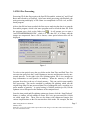
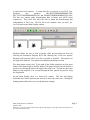
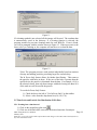
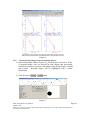
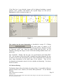
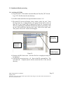
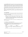
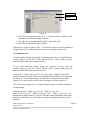
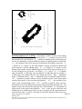
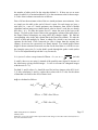
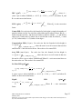
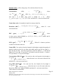
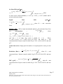
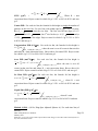
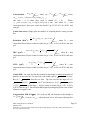
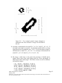
3022 Sterling Circle – Suite 200, Boulder, CO 80301 Phone (303) 449-1105 Fax (303) 449-0132 www.specinc.com 2D-S Post Processing Using 2D-S View Software User Manual Version 1.1 February 2011 Using 2D-S View Software The 2D-S Data Processing Software is constantly being updated. We urge users to consult with SPEC on the current status of the software before beginning processing and periodically. 1.0 2D-S Pre-Processing .........................................................................................3 1.1 Masked diode filling .............................................................................5 1.2 Dead diode replacement ........................................................................6 2.0 2D-S View ........................................................................................................7 2.1 2D-S_View installation .........................................................................7 2.2 More pre-processing .............................................................................9 2.3 Viewing Images ....................................................................................12 2.4 Artifact Removal ...................................................................................13 2.5 Time Series and Particle Size Distribution (PSD) Plots .......................14 2.5.1 Zooming into a time interval..................................................14 2.5.2 Comparing time series ...........................................................16 2.5.3 Comparing size distributions .................................................17 2.5.4 Viewing the 2D-S images from a selected time interval .......18 2.5.5 Boolean Filter.........................................................................19 3 2D-S Data Batch processing (Archiving) ............................................................21 3.1 Liquid mode Batch processing..............................................................22 3.1.1 Archiving ASCII Files ...........................................................22 3.1.2 Archiving Images ...................................................................24 3.1.3 Combining the archived liquid ASCII files ...........................24 3.1.4 Additional Notes ....................................................................25 3.2 Ice mode Batch processing ...................................................................26 3.2.1 Archiving Ice ASCII Files .....................................................26 3.2.2 Archiving Images ...................................................................28 3.2.3Combining the archived Ice ASCII files .................................29 3.2.4 Additional Notes ....................................................................29 Appendix A: Derived Parameters, Methods, Equations in 2D-SView ..................31 Appendix B: Artifact removal algorithm ...............................................................41 SPEC Using 2D-S View Software Page 2 February 2011 SPEC Inc. reserves the right to make improvements and changes to the 2D-S and related software at any time and without notice. 1.0 2D-S Pre-Processing Processing 2D-S data first requires the Spec2D Executable, written in C and Visual Basic and referred to as Playback. After some initial processing with Playback, the main processing and display of 2D-S data is accomplished via 2D-S view, an IDLbased program. After a data file has been recorded, the first step to analyzing the data is to open the Executable program, which is the same program used to record the data file. With the program open, click on the folder icon . It will prompt you to open a ‘baseYYMMDDHHMMSS.2DS’, which is a raw data file. It is binary and the images are compressed. Once a file is chosen, a time period selector box will be displayed. Figure 1 To select a time period, move the two sliders on the Start Time and End Time. For an exact time period use the U and D buttons to increase and decrease time by onesecond intervals. To the right is the File Splitting option. 2D-S view attempts to keep information on each particle in memory. When the memory is full, the program slows due to the use of virtual memory. This can result in unacceptably slow processing. This can be remedied by enabling file splitting, which cuts the original large data file into processed data files of manageable sizes, according to a preset number of particles. A typical setting is 300,000 particles per file, but the optimum size will depend on the attributes of the computer used. Once the time period and file splitting options are chosen, click the ‘Start Playback’ button. A window will ask whether to create 2D-S view pre-processed files, which are called sorted files. These files are also binary with compressed images, but various simplifications to the file structure have been made. For example, the data SPEC Using 2D-S View Software Page 3 February 2011 SPEC Inc. reserves the right to make improvements and changes to the 2D-S and related software at any time and without notice. is sorted into time sequence. A sorted data file is necessary to run 2D-S view. Playback also produces HK_BINYYMMDDHHMMSS.2DS, HK_TXTYYMMDDHHMMSS.2DS, and PAIRSYYMMDDHHMMSS.2DS files. The first two contain probe housekeeping data in binary and ASCII forms respectively. Thus, these files allow the user to obtain the housekeeping data independently of 2D-S view. The Pair file is now obsolete. Once you click ’yes’ you will return to the Main Display window. Figure 2 Playback allows the user to look at images while pre-processing the data. By selecting the Maximum Playback RUN and choosing one of the two options, Playback will create the 2D-S view files as quickly as possible. This option is to the right of the Help tab. The option to not display timestamps is fastest. The other option is quite slow. To the right of the Folder icon there are four green buttons. The farthest right is the Play button. This button will play the file back at a speed set by clicking the icon to the right of the folder icon. You can use the Pause button to stop playback. You can step through the data, particle by particle, using the Step button. On the Main Display, there is a Stereo Pair counter. This area will display horizontal and vertical particles that arrived at nearly the same time. Clicking the Settings button allows the user to set the detection settings: SPEC Using 2D-S View Software Page 4 February 2011 SPEC Inc. reserves the right to make improvements and changes to the 2D-S and related software at any time and without notice. Figure 3 The Minimum Difference value defines the maximum acceptable difference allowed (in 10 μm slices) between the end points of any two events, one horizontal and one vertical. If they pass this criterion, the images could be stereo and they are displayed. If the size of one of those events is larger than the ‘display lower limit’ setting, then Playback will stop upon displaying the images until the user indicates to continue again. Click Save when you are done, if you have changed the numbers and want the same settings next time. This option is an early attempt at determining stereo particles. It is currently considered obsolete in that more sophisticated determination has been implemented in 2DSview. However, for quicklook purposes, this option can still be useful, especially if a large value is used for the size discriminator. 1.1 Masked diode filling: During data collection, a diode may become noisy. If the condition is serious enough, the real time software will detect this and ignore (mask) the diode. This results in a white line running the length of any particle image that includes the mask diode. Examples are shown in Fig. 1 and Fig. 2. Playback has an option to fill these lines within particle images. Click ‘tool’ then ‘mask bit replacement’, a window entitled ‘Mask Bit Recovery settings’ appears. Enable mask filling here and set the maximum number of consecutive masked diodes that can be filled. Filling these artificial white lines is important for the measurement of area, which also affects length when sizing corrections are used. It is even more important to filled masked diodes when they are the edge diode, since that diode is used to determine if an image is complete or not. --------Image with white stripe SPEC Using 2D-S View Software Page 5 February 2011 SPEC Inc. reserves the right to make improvements and changes to the 2D-S and related software at any time and without notice. . Figure 1: Example of the display used to enable masked diode filling. 1.2 Dead diode replacement Similar to a noisy diode, a dead diode leaves a white line running through particle images. In this case however the real time software cannot detect and mask the diode. Therefore playback has an option to add a diode to the mask during preprocessing. The dead diode must be identified first. This is accomplished via the ‘Pixel histogram analysis’ window (Fig. 3). The number of counts each diode has had is displayed. Clicking in a numbered box turns it yellow and indicates that that diode will be considered masked for the next time playback is run. That is, adding diodes to the mask is a two-step process. First, for the period being processed, you must run playback, monitor the histogram of counts display and click on any diodes that you want added to the mask. Next, exit and restart playback, the clicked boxes remain yellow and this time they will be added to the mask for processing. If a noisy diode is not detected and masked during data collection, it may be detected during these same steps and also added to the mask. This can shorted the time needed for 2D-S_view to process as it must also remove noisy diode effects. SPEC Using 2D-S View Software Page 6 February 2011 SPEC Inc. reserves the right to make improvements and changes to the 2D-S and related software at any time and without notice. Figure 3: Example of the ‘Pixel histogram analysis’ window showing a couple dead diodes (V-12 and V-117) and a detectable noisy diode (V-124). 2.0 2D-S View 2.1 2D-S_View Installation 2D-S_view runs on an IDL platform of 6.0 or higher. The projects programs should be stored in a folder called 2DSview-version#. To install the 2D-S view software, follow these steps: 1. Open IDL SPEC Using 2D-S View Software Page 7 February 2011 SPEC Inc. reserves the right to make improvements and changes to the 2D-S and related software at any time and without notice. 2. Click FilePreferencesPath and set the path to the 2DSview-version# folder first and IDL default second. The window should look similar to the one below. Figure 4 3. Click OK 4. In the command line at the bottom of the window type: @compile2dsview Enter. 5. Type in the command line: a2dsviewEnter. The following GUI window will open up: SPEC Using 2D-S View Software Page 8 February 2011 SPEC Inc. reserves the right to make improvements and changes to the 2D-S and related software at any time and without notice. Figure 5 2.2 More pre-processing Before performing quantitative analysis some additional pre-processing steps must be done. First .BIN files are needed: 1. Click the left folder icon . This Brings up a list of all the sorted files created during the playback. 2. Select the SORTED file with the desired time interval. 3. Once the file is loaded a window displaying warning messages will pop up. There may be messages regarding time inconsistencies found while processing the sorted file. Usually there are no messages as the case shown in Fig. 6. Figure 6: Example of a warming messages window. Once a file is selected, a status bar in the lower left of the GUI window shows the number of particles counted. The program will automatically generate the files required. All the .BIN files are placed into a subdirectory labeled, “data”. This process is only required one time for each sorted file. The program automatically looks in the data subdirectory and uses the appropriate .BIN file if it already exists from a previous running. SPEC Using 2D-S View Software Page 9 February 2011 SPEC Inc. reserves the right to make improvements and changes to the 2D-S and related software at any time and without notice. *Note: Due to file size, the time to create .BINS can be quite extensive, but must be done for each SORTED file. To continue, open a .BIN file: 1. Click the right Folder icon 2. Open the Data folder 3. Select a *.BIN for the desired time Again additional files are created in the data subfolder if they do not already exist. These are 1 Hz data files. There will be several pop-up windows depicting the raw data, and the images are automatically saved in the data folder. These auto-saved files are labeled: horiz*.png. Figure 7 is an example of the type of window that will appear. The images can be viewed at any point from this point forward. These are created primarily for SPEC programmers to detect and debug idiosyncratic corrupted data problems. Figure 7 SPEC Using 2D-S View Software Page 10 February 2011 SPEC Inc. reserves the right to make improvements and changes to the 2D-S and related software at any time and without notice. 4. Again a warning messages window pops up showing warnings of idiosyncratic data events. This window is rarely empty but usually has several to a few dozen events. An example is shown in Fig. 8. Figure 8: Example of the warning messages window that pops up after loading the bin files. Once this is completed, three time series are displayed for concentration, extinction, and ice water content (see figure 9). If the file contains more than 300 seconds, the data is coarsely binned into 300 segments for quick look, using the 1 Hz data file that was generated upon opening the .BIN file. If the file is less than 300 seconds then the 1 Hz data is used directly. These 1 Hz data are for quick look only. The processing uses a crude length parameter (L1, see appendix A) and no artifact rejection. SPEC Using 2D-S View Software Page 11 February 2011 SPEC Inc. reserves the right to make improvements and changes to the 2D-S and related software at any time and without notice. Figure 9 By default, the horizontal array time series are displayed. The arrays can be switched by clicking on the (vertical) or (horizontal) icons located on the upper toolbar. 2.3 Viewing Images To view the particle images before artifact rejection has been applied: 1. Choose the desired array either vertical or horizontal 2. Move the cursor over any one of the three plots near the time you want to view 3. Single click, a window similar to Figure 10 will open. SPEC Using 2D-S View Software Page 12 February 2011 SPEC Inc. reserves the right to make improvements and changes to the 2D-S and related software at any time and without notice. Figure 10 The arrows are used for changing the time interval. The single arrow icons allow for moving the view one strip at a time. The icons with two arrows fast forward and rewind. The drop down list to the left of the arrows controls the length of time each strip is in the window while fast forwarding and rewinding. Placing the cursor over single particles displays the size and other parameters in the lower left hand corner. An enlarged image of the particle is displayed, as shown in Figure 10. 2.4 Artifact Removal The .BIN files contain all the data captured by the 2D-S Probe. This includes: noise, splashed, and shattered events, as well as valid images. The program has the ability to remove unwanted data. Using the cleaning functions creates concentrated data for the time series and particle size distribution plots. Before quantitative analysis, there are two options for data filtering: Clean all: Removes noise, shattering, and splashing. Clean noise: Removes noise only. To use the cleaning functions: 1. Specify the type of cleaning by clicking the corresponding icon on the toolbar. 2. A text box will ask for an aspect ratio, as shown in figure 11. If the cloud is known to be liquid enter in 2.0. If the cloud is known to be ice enter a larger value. SPEC Using 2D-S View Software Page 13 February 2011 SPEC Inc. reserves the right to make improvements and changes to the 2D-S and related software at any time and without notice. Figure 11 If a cleaning method is not selected, all the images will be used. The resultant data is automatically saved in the directory. If a cleaning function is selected, the program searches for previous cleanings made for each .BIN file. If one is found, you will be prompted with the window shown in Figure 12. If the aspect ratio is the same, select yes. In doing so, the computer will not have to re-clean the data. Figure 12 *Note: The program processes each particle individually based on statistics of many surrounding particles; processing large files can take days. The In Focus Only feature allows for further data filtering. This removes the particles with holes in them. If the area of the hole is greater than the specified size, the particle is eliminated from the data. For example, if 0.9 is the selected criteria, then only those images with holes having less than 10% of the total area will be used in the process. To use the In Focus Only Feature: 1.) Check the box to the left of “Use In Focus Only” on the toolbar. 2.) Select a value from the drop down list (0.9, 0.8, 0.70). 2.5 Time Series and Particle Size Distribution (PSD) Plots 2.5.1 Zooming into a time interval 1.) Click on the magnifying glass icon . 2.) Click one of the three time series near the desired start time for analysis. SPEC Using 2D-S View Software Page 14 February 2011 SPEC Inc. reserves the right to make improvements and changes to the 2D-S and related software at any time and without notice. 3.) Click the desired end time for analysis. This creates a smaller time interval to be examined. Choosing small time periods significantly reduces subsequent processing time. Similar to the previous window, this new window initially displays concentration, extinction, and ice water content, read from the 1 Hz data file described above, on single time series plots (both H and V are shown simultaneously here). Figure 13 shows the zoomed-in data window. Hi-Res UPDATE Figure 63 PSDs are plotted as well. To view them, click on the Particle Size Dist. Plots tab. These are also crude quick look products using 1Hz data files. The zoomed-in data window allows for a much more in-depth data analysis. In order to access these options select Hi-Res, and click UPDATE. The start and end times can be changed by typing new time values in the Stime and Etime boxes and clicking the UPDATE button. SPEC Using 2D-S View Software Page 15 February 2011 SPEC Inc. reserves the right to make improvements and changes to the 2D-S and related software at any time and without notice. To save any time series or PSD plot as an image, click the Save.png button in the drop list. To save the plot as an ASCII file, click the Save.ascii button. To print a plot, click the Print button. The “ST” button on the left is for displaying stereo images, which is currently not used. The “HK” is for displaying the Housekeeping data. Figure 14 is an example of the plots obtained by selecting HK. This data is used primarily by SPEC Inc. It can also be used for troubleshooting. Figure 14 *Note: Click update after changing any options in the zoomed data window. 2.5.2 Comparing time series Use the CompTMS button to compare time series parameters. In this window, different sizing methods, arrays, and parameters can be plotted and compared. Sizing methods are described in Appendix A. ASCII and image files can be saved from this window. SPEC Using 2D-S View Software Page 16 February 2011 SPEC Inc. reserves the right to make improvements and changes to the 2D-S and related software at any time and without notice. Figure 15 2.5.3 Comparing size distributions Use the CompPSD button to compare particle size distributions. In this window, different sizing methods, arrays, and parameters can be chosen, plotted and compare. Sizing methods are described in Appendix A. Furthermore, average values of counts, concentration, extinction and ice water content will be plotted when applicable. SPEC Using 2D-S View Software Page 17 February 2011 SPEC Inc. reserves the right to make improvements and changes to the 2D-S and related software at any time and without notice. Figure 16 2.5.4 Viewing the 2D-S images from a selected time interval 1.) In the zoomed data window (Figure 13), check the box to the left of ‘Filter’ if accepted images only are desired (for both display and processing). Unclick the filter box to process and display using all the images accepted and rejected. Rejected images will be highlighted with a yellow background. 2.) Click the desired or button. Figure 17 SPEC Using 2D-S View Software Page 18 February 2011 SPEC Inc. reserves the right to make improvements and changes to the 2D-S and related software at any time and without notice. If the filter box is not checked, images will be displayed including: accepted particles, noise, splashes, and shatters. The rejected images are red and are highlighted in yellow as shown in figure 18. Figure 18 This window has the same functionality as described in section 2.3. Clicking will cause pages of images to be displayed on the computer screen saved to the data/png directory. Buttons “cleaning by Start-end clicks” and “label_one_image_as_bad_with_one_click” are for manually removing bad images or noise if the auto-cleaning method doesn’t do a perfect job. The “Timeshift”, “fishing” and “De_spur” are special buttons used inside SPEC INC. We use them to look at the H and V-channel laser beam alignment. We also use them to look at the cloud particle special cluster distribution and to study the noise image distribution in the initial stage of the software. They are for development and automatic removal of noise, splashes and shattering. You do not need to use them. 2.5.5 Boolean Filtering The Boolean feature allows for further sub setting of data. It is possible to filter out particles based on size, location, and various other parameters. To use Boolean filtering: SPEC Using 2D-S View Software Page 19 February 2011 SPEC Inc. reserves the right to make improvements and changes to the 2D-S and related software at any time and without notice. 1.) From the zoomed data window select Boolean On as shown: 2.) Specify the filtering parameter from the drop down list 3.) Use Boolean logic from the drop down list to add filter conditions. 4.) If using numerical values, insert a space between the logic and numerical value. 5.) Hit UPDATE The IDL syntax for the Boolean symbols is defined below: And-And Or-Or Not-Not Eq-Equal to Ne-Not equal to Ge-Greater than or equal to Gt-Greater than Le-Less than or equal to Lt-Less than *-Multiply +-Addition --Subtraction ( )- Used for order of operations For example, if user types “ L1n gt 10” are entered, the filter box is checked and the Update button is clicked, only those accepted and rejected particles with size “L1n greater than 10 pixels” will be selected and displayed in the H-strip and V-strip fields. These will also be used to make the time series and PSD plots. Figure 19 shows an example of when “L1n gt 10” was input for updated processing: SPEC Using 2D-S View Software Page 20 February 2011 SPEC Inc. reserves the right to make improvements and changes to the 2D-S and related software at any time and without notice. Figure 19 Another way to filter the data in a very specific way is to use what has been named the in-focus only option. To access this, go back to the first main 2D-S_view window and click the ‘use in focus only’ check box. You must also select a value from the drop down list. Value options are 0.9, 0.8, and 0.7. This filters the data to use only those images that are at least 90% (80 or 70) shaded. This could be accomplished via the Boolean option as well. The difference is that when using the check box, the sample volume is adjusted using depth of Field values for in-focus particles. 3.0 2D-S Data Batch Processing (Archiving) As described in playback processing section 1.0, after many split sorted files are generated the data can be processed in batch mode, allowing the computer to run over night. When processing batches, all the SORTED files are converted to .BINS and an All Clean filter is applied to them. This allows large quantities of data to be processed and filtered for use at a later date. The batch processing can be done in Liquid mode or Ice mode. When the user knows if the 2-DS probe is flying through liquid cloud (by looking at the temperature, or by observing the playback image types), the batch processing should be done in Liquid mode. When the probe is flying in the ice cloud, the user should use Ice mode. SPEC Using 2D-S View Software Page 21 February 2011 SPEC Inc. reserves the right to make improvements and changes to the 2D-S and related software at any time and without notice. 3.1 Liquid mode Batch processing 3.1.1 Archiving ASCII Files 1.) Copy all sorted***.2ds and the associated HK_bin*.2ds, HK_TXT.2ds and Log_TXT*.2ds files into the same directory. 2.) Get IDL started and follow the steps described in section 1.1.1? 3.) The initial GUI screen will appear. Select “archive_multi_Liq_ascii ” from the drop down list. A dialog window will appear for the user to select an input file of type Sorted*.2DS, as displayed in Figure 20. Navigate to the directory containing the SORTED*.2ds data that requires processing. Click on one of the sorted files, and then click “open” on the lower right corner. That “please select a file” window will disappear. .png Drop Down List Select any SORTED .2DS file Figure 20 ASCII Drop down list with Archive option 4.) Return to the IDL front screen. All of the files for overnight processing will be displayed. 5.) If all the files are present, type y Enter in the IDL command line. This will make the computer process all the sorted data files in the selected directory. SPEC Using 2D-S View Software Page 22 February 2011 SPEC Inc. reserves the right to make improvements and changes to the 2D-S and related software at any time and without notice. Figure 21 The sorted files will be processed one at a time in order. Some initial plots and warning messages will pop up, be saved, and deleted. The original GUI screen will remain open and the progress is displayed in the status bar. The IDL standard output screen will also display some steps that the archiving process has reached. Particles Processed Total Particles Current Process File Being Processed Figure 22 The status bar in Figure 22 displays the following information: 1) The V-channel automatic noise removal is being used. 2) Of the 828565 images, it has examined 115000 particles. 3) The end of the third loop noise removal process for the H channel was done at time: Wed Jun 10, 12:52:04 2009; and etc. SPEC Using 2D-S View Software Page 23 February 2011 SPEC Inc. reserves the right to make improvements and changes to the 2D-S and related software at any time and without notice. As each SORTED**.2DS file is processed, many files are generated and saved in sub-directories labeled data1, data2, data3, etc. in the directory where the original SORTED***.2DS files are stored. These files are initial plots of the file and warning messages encountered when loading the data file, the auto-clean results and the horiz***.bin and vert**.bin files. The most important two files are H_archive_2DS****_xxxx_Ns.txt and V_archive_2DS****_xxxx_Ns.txt. They are located in the subdirectory png under the data1, data2, data3 and etc. These two files Contain the 1Hz concentration, extinction, ice water content, time series and particle size distributions. The header lines contain the detail data format of the archive file. 3.1.2 Archiving Images After H_archive_2DS_***Ns.txt and V_archive_2DS_***Ns.txt 1Hz archive files are generated for each sorted***.2DS file, the a2dsview software can be used on the data. To archive the images: 1.) Select “Archive_Multi_Liq_png” from the .png drop down list (see Figure 20). 2.) A window will ask how many images per second to archive. This is dependent upon cloud type and computing power. Type the desired number of images per second and press Enter. Only the first images up to that number will be archived each second. The images are saved in the subdirectory png under the corresponding data1, data2, data3 etc. subdirectory. 3.1.3 Combining the archived liquid ASCII files To combine all the smaller archive files into a single data file for the whole flight, a separate IDL program is used. To combine all ASCII files follow these steps: 1.) Copy all H_archive_2DS**_Ns.txt into one folder or directory. 2.) Start IDL 3.) Click File Open (Find 2dsview_ver#)combine_Liq_Ns_archive_61bins_HorV.pro 4.) Click Run Compile combine_Liq_Ns_archive_61bins_HorV.pro (Ctrl+F5) 5.) Click Run Run combine_Liq_Ns_archive_61bins_HorV.pro (F5) SPEC Using 2D-S View Software Page 24 February 2011 SPEC Inc. reserves the right to make improvements and changes to the 2D-S and related software at any time and without notice. Step 4 Step 5 Figure 23 6.) You will be prompted to select H or V. This determines whether it is the horizontal or vertical files being combined. 7.) Go to the directory containing the filesand select a file. 8.) In the IDL command line type yEnter From then on, all the H_archive_2DS_***.Ns.txt files will be read and combined in a single archive file, saved in the same directory as the smaller archive files. 3.1.4 Additional Notes To batch archive with the clean option of removing noise only, you should click the “archive_multi_Liq_ascii_WS” button instead of the “archive_multi_Liq_ascii” button and follow the same instructions above. To do batch archiving without doing any removal of noise, click the “archive_multi_Liq_ascii_NC” button instead of the “archive_multi_Liq_ascii” button and follow the same instructions above. Clicking the “ Archive_this_liq_ascii” or “archive_this_Liq_png” in the initial zoomed window will archive the current loaded data file in what ever cleaning state the data is in. If it is cleaned already, it will archive it using only the accepted images. If it is not cleaned, it will use all of the images to do the archive etc. The “make_multi_pbyp_asciis” is a spare button for future use and it currently has no functionality. Clicking any of the “ Make_N_ascii_Liq”, “Make_N_ascii_ice”, “ Make_N_ascii_Liq_WS”, “Make_N_ascii_ice_WS”, “ Make_N_ascii_NC” will batch-generate many zoomed***.txt ascii files that contain information about each particle in each line for users to do their own data processing and analysis, if they choose to. SPEC Using 2D-S View Software Page 25 February 2011 SPEC Inc. reserves the right to make improvements and changes to the 2D-S and related software at any time and without notice. 3.2 Ice mode Batch processing 3.2.1 Archiving Ice ASCII Files 1. Copy all sorted***.2ds and the associated HK_bin*.2ds, HK_TXT.2ds and Log_TXT*.2ds files into the same directory. 2. Get IDL started and follow the steps described in section 1.1.1 3. The initial GUI screen will appear. Select “archive_multi_Ice_ascii ” from the drop down list. A dialog window will appear for the user to select an input file of type Sorted*.2DS as displayed in Figure 20. Navigate to the directory containing the SORTED*.2ds requiring processing. Click on one of the sorted files, and then click “open” on the lower right corner. That “please select a file” window will disappear. .png Drop Down List Select any SORTED .2DS file Figure 24 ASCII Drop down list with Archive option 4. A pop up window with the ice archiving options is shown in Figure 25. See Appendix A for a description of the options. Figure 25 5. Click Accept SPEC Using 2D-S View Software Page 26 February 2011 SPEC Inc. reserves the right to make improvements and changes to the 2D-S and related software at any time and without notice. 6. Return to the IDL front screen. All of the files for overnight processing will be displayed. 7. If all the files are present, type y Enter in the IDL command line. This will make the computer process all the sorted data files in the selected directory. Figure 26 The sorted files will be processed one at a time in order. Some initial plots and warning messages will pop up, be saved, and deleted. The original GUI screen will remain open where the progress is displayed in the status bar. The IDL standard output screen will also print out some of the steps the archiving the process has reached. SPEC Using 2D-S View Software Page 27 February 2011 SPEC Inc. reserves the right to make improvements and changes to the 2D-S and related software at any time and without notice. Particles Processed Total Particles Current Process File Being Processed Figure 27 The status bar in figure 27 gives the following information: 1) The Vchannel automatic noise removal is being used. 2) Of the 828565 images, it has examined 115000 particles. 3) The end of the third loop noise removal process for the H channel was done at time: Wed Jun 10, 12:52:04 2009. As each SORTED**.2DS file is processed, many files are generated and saved in a sub-directory labeled data1, data2, data3, etc. in the directory where the original SORTED***.2DS files are stored. These files are initial plots of the file, warning messages encountered when loading the data file, the auto-clean results and the horiz***.bin and vert**.bin files. The most important two files are H_archive_2DS****_xxxx_Ns.txt and V_archive_2DS****_xxxx_Ns.txt. They are located in the subdirectory png under the data1, data2, data3 and etc. These two files contain the 1Hz concentration, extinction, ice water content, times series and particle size distributions. The header lines contain the detail data format of the archived file. 3.2.2 Archiving Images After H_archive_2DS_***Ns.txt and V_archive_2DS_***Ns.txt 1Hz archive files are generated for each sorted***.2DS file, the a2dsview software can be used on the data. To archive the images: 1. Select “Archive_Multi_Ice_png” from the .png drop down list (see Figure 20). 2. A window will ask how many images per second to archive. This is dependent upon cloud type and computing power. Type in the desired number of images per second and press Enter. The images are saved in the subdirectory .png under the corresponding data1, data2, data3 etc subdirectory. SPEC Using 2D-S View Software Page 28 February 2011 SPEC Inc. reserves the right to make improvements and changes to the 2D-S and related software at any time and without notice. 3.2.3 Combining the archived Ice ASCII files To combine all the smaller archive files into a single data file for the whole flight, a separate IDL program is used. To combine all ASCII files follow these steps: 1. Copy all H_archive_2DS**_Ns.txt into one folder or directory. 2. Start IDL 3. ClickFileOpen(Find2dsview_ver#)combine_archive_TC4_St eve_gains_of_61bins_HorV.pro. 4. ClickRunCompilecombine_archive_TC4_Steve_gains_of_61bins _HorV.pro. (Ctrl+F5) 5. Click Run Run combine_archive_TC4_Steve_gains_of_61bins_HorV.pro. (F5) Step 4 Step 5 Figure 28 6. A prompt you to select H or V, this determines whether it is the horizontal or vertical files being combined. 7. Go to the directory containing the filesselect a file. 8. In the IDL command line type yEnter From then on, all the H_archive_2DS_***.Ns.txt files will be read and combined in a single archive file, saved in the same directory as the smaller archive files. 3.2.4 Additional Notes To batch archiving with the clean option of removing noise only, you should click the “archive_multi_Ice_ascii_WS” button instead of the “archive_multi_Ice_ascii” button and follow the same instructions as above. SPEC Using 2D-S View Software Page 29 February 2011 SPEC Inc. reserves the right to make improvements and changes to the 2D-S and related software at any time and without notice. To do batch archiving without removing noise, you should click the “archive_multi_Ice_ascii_NC” button instead of the “archive_multi_Ice_ascii” button and follow the same instructions above. Clicking the “ Archive_this_Ice_ascii” or “archive_this_Ice_png” in the initial zoomed window will archive the current loaded data file in whatever cleaning state the data is in. If it is cleaned already, it will archive it using only the accepted images. If it is not cleaned, it will use all images to do the archive, etc. The “make_multi_pbyp_asciis” is a spare button for future use and it currently has no function. Clicking any of the “ Make_N_ascii_Liq”, “Make_N_ascii_ice”, “ Make_N_ascii_Liq_WS”, “Make_N_ascii_ice_WS”, “ Make_N_ascii_NC” will batch generate many zoomed***.txt ascii files that contain information of each particle, in each line for users to do their own data processing and analysis, if they choose to. SPEC Using 2D-S View Software Page 30 February 2011 SPEC Inc. reserves the right to make improvements and changes to the 2D-S and related software at any time and without notice. Appendix A: Derived Parameters, Methods, Equations in 2DSView Derived parameters are as follows: ‘Timestamp’, ‘Index’ of same event’s image in the sorted file, ‘A1’ = number of shaded pixels, ‘L1’ = number of pixels in TAS direction that the event lasted for, ‘L2’ = number of shaded pixels in array direction for the slice during the event for which the number of shaded pixels is maximized, ‘L3’ = the diameter of the circle that just circumscribes the shaded event pixels. 'L4' = similar to ‘L2’ except it is the total number of pixels between the shaded end pixels instead of just the shaded pixels. 'L5' = is similar to 'L4' except it is the distance between the extreme shaded end pixels from all the slices whereas for 'L4' it is the end pixels in a given slice. See Figure 1. A3 = (/4)L32, ‘F1’ = 0 if neither edge was shaded, 1 if left edge only was shaded, 2 if right edge only was shaded, 3 if both edges were shaded (for any slice during the event), ‘Adj1’ = adjustment factor #1 (defined below), ‘Adjn’ = adjustment factor #n (defined further below), ‘PC1’ = position of particle center on array, determined as the center between the extreme edge points of the slice that determined L2. ‘PC3’ = the position of the center of the circumscribing circle. ‘PC4’ = position of particle center on array, determined as the center between the extreme edge points that determined L5. For logistic reasons, the derived files will also have TAS included. L6 = the number of white pixels in the strip(s) that defined L4. So L4 is the strip for which the end shaded pixels are farthest apart which can be a surrogate for the outer diameter of an out of focus ring. L6 then is a surrogate for the inner diameter of the ring as it is SPEC Using 2D-S View Software Page 32 February 2011 SPEC Inc. reserves the right to make improvements and changes to the 2D-S and related software at any time and without notice. the number of white pixels for the strip that defined L4. If there are two or more strips for which L4 is maximized then let L6 be the maximum value for those strips. L7 is the Alexei scheme corrected size as follows: First of all use the maximum value of the two inside-perimeter area estimates. Next we simply use the table at the end of Alexei’s report. For each image we have a total area (A2 = max of 2 inside perimeter area estimates, from Alexei’s Matlab algorithm) and an image area (shaded pixels, also in Alexei’s code but we already have this = A1). We take the square root of 1 minus the ratio of the later to the former. We look up the closest value in the appropriate column of the table (that is the Dspot/ Dmax column)(we are using table 40% shadow depth). We find the corresponding value in the 2nd column (that is the Dmax/Do column). We take the inverse of that and multiply by Dmax to obtain Do, which is our corrected size estimate for the bead. If the corrected size (Do) is larger than the original size (Dmax), do not use the correction! use Dmax instead. For round images Dmax might be better estimated from total area but for the bead data we will have to use the along the array size (L4) as the bead's speeds through the probe varied (unless TAS is well adjusted and speeds don’t vary too much). L8 is just as L7 above except instead of Dmax = L4, use Dmax 4 A2 * L4 L1 . (in both L7 and L8 above we are using L4 instead of the possibly more logical L5 because of the tilted arrays giving skewed images... L8 tries to account for elongated images with the ratio L4 : L1) For both L7 and L8 above, L4 should be used for in-focus images at the 90% level. I. E. after calculating L7 and L8, replace their values with L4’s value for the subset of data that is in-focus at the 90% or better level. Adj1 is calculated as follows: Adj1 SVdefault SV1 SAdefault SA1 actual actual SVdefault TAS t SAdefault SV1 actual TAS t SA1 actual SPEC Using 2D-S View Software Page 33 February 2011 SPEC Inc. reserves the right to make improvements and changes to the 2D-S and related software at any time and without notice. SV stands for sampled volume (Liters), SA for sample area (mm2), TAS (m/s) the speed of air through the probe sample area, and t (seconds) the time period of the measurement. SAdefault 128 pxs d ww Where ‘pxs’ = 0.01 mm (10 m) is the optically realized size of the array elements and dww = 63 mm (6.3 cm) is the window to window distance. ‘Strbsz’ is the pixel size in the TAS direction (strobe size) and should also = 10 m but could differ if the aircraft flies too quickly or an incorrect TAS is sent to the probe during data acquisition. SA1 actual (127 L1 strbsz/pxs) pxs min[d ww , d of ] where dof stands for depth of field and dof (mm) Fdof L1 strbsz2 ( m2 ) / 1000. 2 -1 where Fdof = 5.13 (μm ). PC1 can be found as the halfway point between the edge points of the image on the array for the slice that defined L2. PC3 can be found as the center of the circle that defined L3. Methods - Equations: Method 1 (M1): (TAS direction, all particles): For each time bin (of size t), Concentration (#/L) = K Adj1 SV . Where K = unit conversion factor. default Counts time series: the number of particle events per time bin. Extinction (Km-1) = 2 K ( Adj1 Area pxs strbsz) SV Where K = unit default conversion factor. SPEC Using 2D-S View Software Page 34 February 2011 SPEC Inc. reserves the right to make improvements and changes to the 2D-S and related software at any time and without notice. IWC: (g/m3) = K1 ( Adj1 min[ A , i K2 ( L1 strbsz) 3 ]) K1 6 SVdefault where A = (Area x pxs x strbsz)/1000000, = 0.115, = 1.218, i =0.917, and where K1 and K2 are unit conversion factors. 3 LWC: (g/m ) = K ( Adj1 6 ( L1 strbsz) 3 ) SVdefault . Where K2 is unit conversion factor. Counts PSD: For each size bin, the formula for bin height is simply the number of particles in that size bin. Use size bins with width equal to strbsz for now. Bin (L1 strbsz) into the size bins. The first size bin has events for which L1 = 1 and the bin edges are 0.5*strbsz and 1.5*strbsz, the nth size bin has events for which L1 = n and (n - 0.5)*strbsz and (n + 0.5)*strbsz as bin edges.... Concentration PSD (#/L/m): For each size bin, the formula for bin height is K ( Adj1 ) (bin _ width( m) SVdefault ) where the sum is over all events in that size bin and Where K = unit conversion factor. Bin as above for counts PSD. Area PSD (mm2/L/m): K ( Adj1 ) A For each size bin, the formula for bin height is (bin _ width( m) SVdefault ) where the sum is over all events in that size bin and A=(Area x pxs x strbsz)/1000000 and Where K = unit conversion factor so the units come out. Bin as above for counts PSD. Ice Mass PSD (g/m3/m): K1 ( Adj1 min[ A , i K2 ( L1 strbsz) 3 ]) K1 6 (bin _ width( m) xSV default ) where A=(Area x pxs x strbsz)/1000000, = 0.115, = 1.218, i = 0.917, and where K1 and K2 are unit conversion factors. Liquid K ( Adj1 6 Mass PSD ( L1 strbsz) 3 ) (bin _ width( m) SVdefault) (g/m3/m): Where K = unit conversion factor. SPEC Using 2D-S View Software Page 35 February 2011 SPEC Inc. reserves the right to make improvements and changes to the 2D-S and related software at any time and without notice. Method 2 (M2): (All in, along array): For each time bin (of size t), Concentration Adj 2 (#/L) SVdefault SV2 SAdefault SA2 actual K Adj 2 = where SA2 actual where SVdefault (127 - L4 ) pxs min[d ww , d of _ 2 ] actual and Adj2 = 0 if either edge pixel is shaded (F1 ≠ 0). Where 2 1 2 2 d of _ 2 (mm) 5.13( m ) L4 pxs ( m )/ 1000. and where K = unit conversion factor. Counts time series: the number of particle events per time bin. Extinction (Km-1) = 2 K ( Adj 2 Area pxs strbsz) SV where K = unit default conversion factor. 3 IWC: (g/m ) = K1 ( Adj 2 min[ A , i K2 ( L4 pxs ) 3 ]) K1 6 SVdefault where A=(Area x pxs x strbsz)/1000000, = 0.115, = 1.218, i = 0.917, and K2 and K1 are unit conversion factors. 3 LWC: (g/m ) = K ( Adj 2 6 ( L4 pxs ) 3 ) SVdefault . Where K = whatever you have to make it so the units come out. Counts PSD: For each size bin, the formula for bin height is simply the number of particles in that size bin. Use size bins with width equal to pxs for now. Bin (L2 pxs) into the size bins. The first size bin has events for which L2 = 1 and the bin edges are 0.5* pxs and 1.5* pxs, the nth size bin has events for which L2 = n and (n 0.5)* pxs and (n + 0.5)* pxs as bin edges.... Concentration PSD (#/L/m): For each size bin, the formula for bin height is K ( Adj 2 ) (bin _ width( m) SVdefault ) where the sum is over all events in that size bin and where K = unit conversion factor. Area PSD (mm2/L/m): K ( Adj 2 ) A For each size bin, the formula for bin height is (bin _ width( m) SVdefault ) where the sum is over all events in that size bin and A=(Area x pxs x strbsz)/1000000 and where K = unit conversion factor. Bin as above for counts PSD. SPEC Using 2D-S View Software Page 36 February 2011 SPEC Inc. reserves the right to make improvements and changes to the 2D-S and related software at any time and without notice. Ice Mass PSD (g/m3/m): K1 ( Adj 2 min[ A , i K2 ( L4 pxs ) 3 ]) K1 6 (bin _ width( m) SVdefault ) where A=(Area x pxs x strbsz)/1000000, = 0.115, = 1.218, i = 0.917, and K2 and K1 are unit conversion factors. Liquid Mass K ( Adj 2 6 (g/m3/m): PSD ( L4 pxs ) 3 ) (bin _ width( m) SVdefault) where K = unit conversion factor. Method 3 (M3): (All in, simple non-adjusted spheres): For each time bin (of size t), Adj3 concentration SVdefault SV3 SAdefault SA3 actual K Adj 3 = SVdefault where where actual SA3actual (127 - L3 ) min[ pxs , strbsz] min[d ww , d of _ 3 ] and Adj3 = 0 if either edge pixel is shaded (F1 ≠ 0). Where d of _ 3 (mm) 5.13( m 1 ) ( L3 ) 2 min[ pxs , strbsz]2 ( m 2 )/ 1000. and where K = unit conversion factor. Reject events for which L4 gt 2.1*L1 or L4 lt 0.49*L1 and area gt 2. Counts time series: Simply plot the number of accepted particle events per time bin. -1 Extinction (Km ) = 2 K ( Adj 3 L23 pxs strbsz) SVdefault where K = unit conversion factor. Rejects events for which L4 gt 2.1*L1 or L4 lt 0.49*L1 and area gt 2. 3 IWC: (g/m ) = 0.917 K ( Adj 3 6 3 L3 pxs strbsz ) SVdefault where K = unit conversion factor. Reject events for which L4 gt 2.1*L1 or L4 lt 0.49*L1 and area gt 2. SPEC Using 2D-S View Software Page 37 February 2011 SPEC Inc. reserves the right to make improvements and changes to the 2D-S and related software at any time and without notice. 3 LWC: (g/m ) K ( Adj 3 = 6 3 L3 pxs strbsz ) SVdefault Where K = unit conversion factor. Reject events for which L4 gt 2.1*L1 or L4 lt 0.49*L1 and area gt 2. Counts PSD: For each size bin, the formula for bin height is simply the number of particles in that size bin. Use size bins with width equal to pxs strbsz for now. Bin (L3 pxs strbsz ) pxs strbsz and 1.5* into the size bins. The first size bin has edges of 0.5* pxs strbsz , the nth size bin has (n - 0.5)* pxs strbsz and (n + 0.5)* pxs strbsz as bin edges. Reject events for which L4 gt 2.1*L1 or L4 lt 0.49*L1 and area gt 2. Concentration PSD (#/L/m): For each size bin, the formula for bin height is K ( Adj 3 ) (bin _ width( m) SVdefault ) where the sum is over all events in that size bin and where K = unit conversion factor. Bin as above for counts PSD. Reject events for which L4 gt 2.1*L1 or L4 lt 0.49*L1 and area gt 2. Area PSD (mm2/L/m): 2 For each size bin, the formula for bin height is K ( Adj 3 L pxs strbsz) 2 3 (bin _ width( m) SVdefault ) where the sum is over all events in that size bin and where K = unit conversion factor. Bin as above for counts PSD. Reject events for which L4 gt 2.1*L1 or L4 lt 0.49*L1 and area gt 2. Ice Mass PSD (g/m3/m): For each size bin, the formula for bin height is 0.917 K ( Adj 3 6 3 L3 pxs strbsz ) (bin _ width( m) SVdefault ) where K = unit conversion factor. Reject events for which L4 gt 2.1*L1 or L4 lt 0.49*L1 and area gt 2. Liquid Mass PSD (g/m3/m): K ( Adj 3 6 3 L3 pxs strbsz ) (bin _ width( m) SVdefault ) where K = unit conversion factor. Reject events for which L4 gt 2.1*L1 or L4 lt 0.49*L1 and area gt 2. Method 4 (M4): (All In, Ring-Spot Adjusted Spheres A): For each time bin (of size t), SPEC Using 2D-S View Software Page 38 February 2011 SPEC Inc. reserves the right to make improvements and changes to the 2D-S and related software at any time and without notice. Concentration = K Adj 4 SV where Adj 4 default SVdefault SV4 SAdefault SA4 actual where actual SA4actual (127 - L7 ) min[ pxs , strbsz] min[d ww , d of _ 4 ] and Adj4 = 0 if either edge pixel is shaded (F1 ≠ 0). Where 1 2 2 2 d of _ 4 (mm) 5.13( m ) ( L7 ) min[ pxs , strbsz] ( m )/ 1000. and where K = unit conversion factor. Also reject events for which L5 gt 2.1*L1 or L5 lt 0.49*L1 and area gt 2. Counts time series: Simply plot the number of accepted particle events per time bin. -1 Extinction (Km )= 2 K ( Adj 4 L27 pxs strbsz) SVdefault where K = unit conversion factor. Reject events for which L4 gt 2.1*L1 or L4 lt 0.49*L1 and area gt 2. 3 IWC: (g/m ) = 0.917 K ( Adj 4 6 3 L7 pxs strbsz ) SVdefault where K = unit conversion factor. Reject events for which L4 gt 2.1*L1 or L4 lt 0.49*L1 and area gt 2. 3 LWC: (g/m ) = K ( Adj 4 6 3 L7 pxs strbsz ) SVdefault where K = unit conversion factor. Reject events for which L4 gt 2.1*L1 or L4 lt 0.49*L1 and area gt 2. Counts PSD: For each size bin, the formula for bin height is simply the number of particles in that size bin. Use size bins with width equal to pxs strbsz for now. Bin (L7 pxs strbsz ) into the size bins. pxs strbsz and 1.5* pxs strbsz , th The first size bin has edges of 0.5* the n size bin has (n - 0.5)* pxs strbsz and (n + 0.5)* pxs strbsz as bin edges.... Reject events for which L4 gt 2.1*L1 or L4 lt 0.49*L1 and area gt 2. Do not adjust bin heights by multiplying by the ratio of total events to accepted events. Concentration PSD (#/L/m): For each size bin, the formula for bin height is K ( Adj 4 ) (bin _ width( m) SVdefault ) where the sum is over all events in that size bin SPEC Using 2D-S View Software Page 39 February 2011 SPEC Inc. reserves the right to make improvements and changes to the 2D-S and related software at any time and without notice. and where K = unit conversion factor. Bin as above for counts PSD. Reject events for which L4 gt 2.1*L1 or L4 lt 0.49*L1 and area gt 2. Area PSD (mm2/L/m): 2 For each size bin, the formula for bin height is K ( Adj 4 L27 pxs strbsz) (bin _ width( m) SVdefault ) where the sum is over all events in that size bin and where K = unit conversion factor. Bin as above for counts PSD. Reject events for which L4 gt 2.1*L1 or L4 lt 0.49*L1 and area gt 2. Ice Mass PSD (g/m3/m): For each size bin, the formula for bin height is 0.917 K ( Adj 4 6 3 L7 pxs strbsz ) (bin _ width( m) SVdefault ) where K = unit conversion factor. Reject events for which L4 gt 2.1*L1 or L4 lt 0.49*L1 and area gt 2. Liquid K ( Adj 4 6 Mass (g/m3/m): PSD 3 L7 pxs strbsz ) (bin _ width( m) SVdefault ) where K = unit conversion factor. Reject events for which L4 gt 2.1*L1 or L4 lt 0.49*L1 and area gt 2. Method 5 (M5): (All In, Ring-Spot Adjusted Spheres B): The same as Method 4 above except replace all L7 with L8. Method 6 (M6): (in focus only, combined): This method is for when there are sufficient particles to use in focus only and when there is need to extend to larger sizes than can be adequately sampled by ‘all in’ techniques. It uses M2 in-focusonly after CleanAll for sizes smaller than 265. It uses M1 in-focus-only without cleaning for sizes greater than 325. For sizes between 265 and 325, it uses the average of the preceding two methods. A future improvement should be to replace the M1 part with a reconstruction technique. SPEC Using 2D-S View Software Page 40 February 2011 SPEC Inc. reserves the right to make improvements and changes to the 2D-S and related software at any time and without notice. Appendix B: Removing Spurious 2D-S Events 2D-S raw data include spurious effects. These are primarily from instrument noise and from splashing of precipitation. Algorithms used to clean the data of the majority of these spurious effects while retaining the majority of the valid images are described here. There are 5 quasi independent steps to the algorithm implemented via two loops through the data: First Loop: 1) 2) 3) 4) Test for roundness. Test for splashing events based on black and white area considerations. Test for noise via line and dot patterns. Test for noise via statistics of particle center locations. Second Loop: 5) Test for splashing events based on inter-event-distances if the probe is in precipitation. Each step will be described in detail after defining terms: Four measures of image length are shown in figure A.1. ‘L1’ is the number of slices (pixels in the direction of travel) for which the event lasted. ‘L2’ is the number of shaded diodes (pixels in the direction along the array) for the slice for which the same quantity is maximized. 'L4' is the number of diodes between, and including the shaded end diodes, for the slice that maximizes the same quantity. 'L5' is the distance between (and including) the shaded end diodes considering all of the slices together. Other size parameters are a corrected size for out of focus images based on Korolev 19?? (ref?) (L7), the number of shaded pixels for the entire image (summed over all slices) (As) and an estimate of total number of pixels, shaded or not, for the entire image (At). The algorithm for At is part of the Korolev size correction method. SPEC Using 2D-S View Software Page 42 February 2011 SPEC Inc. reserves the right to make improvements and changes to the 2D-S and related software at any time and without notice. Figure B.1: Two example particle images designed to demonstrate the four measures of image size described in the text. 1) An image is determined to be round if L1 ≥ 0.5 x L5 and L5 ≥ 0.5 x L1. If an image is not round, it is rejected. An exception is made for the very large images that do not fit within the array. If L5 > 50 (500 μm) then an image is determined to be round if L1 ≥ 0.5 x L5. I. E. an image is determined to be round if L1 ≥ 0.5 x L5 and (L5 ≥ 0.5 x L1 or L5 > 50). 2) The larger a valid image is the greater the percentage of shaded pixels. Splash effects often create large images that have lower percentages of shaded pixels than valid images. The follow criteria are used to eliminate such spurious images: i. (L5 > 10 or L1 > 10) and (At > 3.0 X As) ii. (L5 > 15 or L1 > 15) and (At > 2.5 X As) iii. (L5 > 20 or L1 > 20) and (At > 2.0 X As) iv. (L5 > 35 or L1 > 35) and (At > 1.5 X As) v. (L5 > 2.2 X L7) and (L1 > 10.0) SPEC Using 2D-S View Software Page 43 February 2011 SPEC Inc. reserves the right to make improvements and changes to the 2D-S and related software at any time and without notice. If any of these five criteria are met the image is rejected. 3) Figure B.2 shows some examples of noise generated images appearing in line plus dot patterns. Figure B.2: Examples of line plus dot patterns caused by noisy diodes. These are eliminated using the following criteria: i. ii. iii. iv. v. vi. (L1 = As) and (L2 = 1) and (L1 > 4) (As ≤ 1.35 X L1) and (L4 = L5) and (L1 > 4) and (L2 = 2) (L1 > 10) and (L1 > 0.75 X As) and (L1 ≤ 1.5 X As) (L4 = L5) and (At > 0.9 X L1 X L5) and (L2 = 2) and (L2 ≠ L4) (L4 = L5) and (At > 3.0 X As) and (L2 = 2) (L4 = L5) and (At > 4.0 X As) If any of these six criteria are met the image is rejected. 4) The final step, of this first cleaning loop, is another noisy diode removal method, based on the statistics of image center locations calculated over 4000 images1 approximately centered on the image being evaluated. When a diode is noisy there are more image centers located on that diode than are located on quiet diodes. A diode is labeled bad when it has more particle center locations than the threshold value (TH = max ). Where M is the mean number of image centers per diode across the array, for diodes having more than a minimum number of image center counts. This minimum number is , where Mt is the mean number of image centers per diode across the array, for all diodes. If less than 33 diodes satisfy the requirement of having more than Mt counts then M is 1 The 4000 images includes all images, whether rejected by previous steps or not, and is updated every 100 images so that the 4000 images are approximately centered on the current image. If the file contains less than 4000 images then all images are used. 4000 was chosen because of the approximate match between the mean ( 4000 /128= 31 ) and threshold. SPEC Using 2D-S View Software Page 44 February 2011 SPEC Inc. reserves the right to make improvements and changes to the 2D-S and related software at any time and without notice. calculated from all diodes. Mt and M are recalculated after bad diodes are identified, ignoring those diodes, and the process repeated until no diodes exceed the threshold. An image whose center falls on a bad diode is rejected unless it meets one of the following criteria: i. ii. iii. (L1 ≥ 15) and (L5 ≥ 15) and (As > 0.7 X At) (L1 ≥ 4) and (L5 ≥ 4) and (As ≥ 0.5 X At) and (L2 > 0.25 X L5) and (L1 < 50) (L2 = L4) and (L2 = L5) and (L2 ≥ 2) and (As ≥ 0.5 X At) Figure B.3 shows an example of noisy diode data and the distribution of image centers across the array. SPEC Using 2D-S View Software Page 45 February 2011 SPEC Inc. reserves the right to make improvements and changes to the 2D-S and related software at any time and without notice. Figure B.3: Shows an example of noisy diode data intermixed with good particle data. The images highlighted in yellow are rejected. Labels in red point to images centered on diodes determined to be bad (too noisy) by the criteria described in the text and exemplified in the particle center location distribution shown above. 5) This final step is another loop through the data but is applied only if the current precipitation status is ‘yes’. The current precipitation status is ‘yes’ if there is one or more particle(s) with L7 gt 100 microns in the 10000 particles, accepted by the previous 4 cleaning steps, centered approximately on the current particle. It is approximately centered because the precipitation status is updated only every 100 particles, instead of for every particle, to improve speed. Another parameter, the current mean interparticle time (aveW8), is similarly updated every 100 particles and calculated as the average inter-particle time between the 10000 images, accepted by the previous 4 cleaning steps, centered approximately on the current particle. All the particles in the previous second are used instead of 5000 particles if there are less than 5000 particles in the previous second, similarly for the following 5000 particles or second. If aveW8 > 40000 then C1 = 2000 and C2 = 8000. If aveW8 < 40000 then C1 = 0.05 X aveW8 and C2 = 0.2 X aveW8. A particle is rejected if the precipitation status is ‘yes’ and either: a) the particle’s inter-particle time or the following particle’s inter-particle time is less than C1 or b) both the particle’s inter-particle time and the following particle’s inter-particle time are less than C2. Finally, a The precipitation status and current mean waiting time are updated every particle, instead of every 100, if the valid particle rate is slower than 1000 per second, averaged over the surrounding 0.2 seconds. SPEC Using 2D-S View Software Page 46 February 2011 SPEC Inc. reserves the right to make improvements and changes to the 2D-S and related software at any time and without notice. variable, adj0, is calculated for each image. It is 0 for rejected images, 1 for accepted images if precipitation status is ‘no’. When precipitation status is ‘yes’, then for accepted images, we calculate a new true average interparticle time (TaW) = the average inter-particle time of particles accepted by all the steps minus C1. Then calculate k is limited to a maximum of 0.9 and then . adj0 is used elsewhere, in the algorithms for calculating concentrations etc., to increase the weight of each accepted particle to account for those good particles rejected by the inter-particle time criteria. k is the fraction of events eliminated by the criteria given a true waiting time distribution with mean of TaW. is the probability of, or fraction of events with, inter-arrival times less than C1. is the fraction of events eliminated due to the first criteria, leaving not eliminated by the first criteria. Of those, a fraction are eliminated by the second criteria. SPEC Using 2D-S View Software Page 47 February 2011 SPEC Inc. reserves the right to make improvements and changes to the 2D-S and related software at any time and without notice. Appendix C: Updating the 2DS Real-Time/Post Processing program The 2DS Real-Time and Playback program is installed to a computer by an executable install program. The program then needs to be updated with the latest version. When SPEC releases a new version the executable needs to be replaced in the Program Files/SPEC, Inc/SPEC2DS folder. Occasionally another file, SPEC2DS.ocx, located in the WINNT/system32 folder needs to be replaced. In order to replace it you need to unregister the previous version and then copy over the file and re-register it. To do this click on Windows Start button and click Run. In command line type: Regsvr32 /u c:\winnt\system32\spec2ds.ocx A box should pop up confirming the registry change was successful. Copy in new .ocx file and type: Regsvr32 c:\winnt\system32\spec2ds.ocx After another confirmation, the program is updated. Installing 2DSview: 2DSview comes in a folder; the only step to installing 2DSview is to set the IDL path to this folder. Open Project file and follow directions as detailed in Section 6.1