Download Downloads - CompChemMPI

Manual
Computational Physical Chemistry
- SCRIPTS and TOOLS for and INFORMATION on Running and Analysing Molecular
Dynamics Simulations Kathleen Kirchner
Physics and Life Sciences, Nanoscience Division, Department of Physics, Strathclyde
University, G4 0NG Glasgow, U.K.
April 14, 2012
Short summary
This document should provide the reader with detailed information on starting and analysing
molecular dynamics simulations with GROMACS. It is a collection of scripts and experiences
that have been made by Andrey Frolov and Kathleen Kirchner under the supervision and
with the help of Prof Dr Maxim Fedorov starting from the middle of 2008 (begin of Andrey
Frolov’s PhD) till now.
1
Contents
1 System preparation
1.1 Configurations . . . . . . . . . . . . . . . . . . . . . . .
1.1.1 Generation of first coordinates . . . . . . . . . .
1.1.2 Combining them all to full systems under study
1.2 Force fields . . . . . . . . . . . . . . . . . . . . . . . .
1.2.1 Carbon nanoparticles . . . . . . . . . . . . . . .
1.2.2 Organic molecules . . . . . . . . . . . . . . . . .
1.2.3 Charges . . . . . . . . . . . . . . . . . . . . . .
.
.
.
.
.
.
.
.
.
.
.
.
.
.
.
.
.
.
.
.
.
.
.
.
.
.
.
.
.
.
.
.
.
.
.
.
.
.
.
.
.
.
.
.
.
.
.
.
.
2 Running simulations with Gromacs
2.1 Molecular dynamics parameter file .mdp . . . . . . . . . . . . . . .
2.2 Running Gromacs . . . . . . . . . . . . . . . . . . . . . . . . . . . .
2.2.1 Energy minimization and equilibration . . . . . . . . . . . .
2.2.2 Production runs . . . . . . . . . . . . . . . . . . . . . . . . .
2.2.3 Data storage for further analysis . . . . . . . . . . . . . . . .
2.3 Running replicas . . . . . . . . . . . . . . . . . . . . . . . . . . . .
2.3.1 Independent initial configurations by different random seeds
2.3.2 Grabbing frames from a trajectory . . . . . . . . . . . . . .
2.3.3 System heating . . . . . . . . . . . . . . . . . . . . . . . . .
2.4 Computing facilities . . . . . . . . . . . . . . . . . . . . . . . . . . .
2.4.1 Local systems . . . . . . . . . . . . . . . . . . . . . . . . . .
2.4.2 British supercomputer HECToR . . . . . . . . . . . . . . . .
2.4.3 German supercomputer JUROPA . . . . . . . . . . . . . . .
2.5 Comments . . . . . . . . . . . . . . . . . . . . . . . . . . . . . . . .
.
.
.
.
.
.
.
.
.
.
.
.
.
.
.
.
.
.
.
.
.
.
.
.
.
.
.
.
.
.
.
.
.
.
.
.
.
.
.
.
.
.
3 System analysis
3.1 Visual analysis . . . . . . . . . . . . . . . . . . . . . . . . . . . . . . .
3.2 Gromacs tools . . . . . . . . . . . . . . . . . . . . . . . . . . . . . . . .
3.2.1 Density and density profile . . . . . . . . . . . . . . . . . . . . .
3.2.2 Radial distribution function and coordination number . . . . . .
3.2.3 Distribution function in cylindrical geometry . . . . . . . . . . .
3.2.4 Distribution function in slab geometry . . . . . . . . . . . . . .
3.2.5 Order parameter for alkyl chains . . . . . . . . . . . . . . . . .
3.2.6 Order parameter for alkyl chains as a function of box length . .
3.2.7 Head stacking - How to analyse the orientation of aromatic rings
3.2.8 2D number density map . . . . . . . . . . . . . . . . . . . . . .
3.3 Self written scripts . . . . . . . . . . . . . . . . . . . . . . . . . . . . .
3.3.1 Potential of mean force and free energy . . . . . . . . . . . . . .
3.3.2 Orientation analysis . . . . . . . . . . . . . . . . . . . . . . . .
3.3.3 Volumes of solute cavities ToDo . . . . . . . . . . . . . . . . . .
3.3.4 Residence time ToDo . . . . . . . . . . . . . . . . . . . . . . . .
2
.
.
.
.
.
.
.
.
.
.
.
.
.
.
.
.
.
.
.
.
.
.
.
.
.
.
.
.
.
.
.
.
.
.
.
.
.
.
.
.
.
.
.
.
.
.
.
.
.
.
.
.
.
.
.
.
.
.
.
.
.
.
.
.
.
.
.
.
.
.
.
.
.
.
.
.
.
.
.
.
.
.
.
.
.
.
.
.
.
.
.
.
.
.
.
.
.
.
.
.
.
.
.
.
.
.
.
.
.
.
.
.
.
.
.
6
6
6
7
9
9
9
11
.
.
.
.
.
.
.
.
.
.
.
.
.
.
12
12
13
14
14
15
15
15
15
15
16
16
17
19
19
.
.
.
.
.
.
.
.
.
.
.
.
.
.
.
20
20
20
20
21
23
23
24
24
24
25
25
25
25
27
27
4 Plotting, fitting and statistical analysis
4.1 General comments on figures . . . . . .
4.2 Plotting data . . . . . . . . . . . . . .
4.2.1 Grace (Xmgrace) . . . . . . . .
4.2.2 Matlab . . . . . . . . . . . . . .
4.3 Fitting data . . . . . . . . . . . . . . .
4.3.1 Matlab . . . . . . . . . . . . . .
4.4 Statistical analysis ToDo . . . . . . . .
4.4.1 Matlab . . . . . . . . . . . . . .
4.4.2 R . . . . . . . . . . . . . . . . .
.
.
.
.
.
.
.
.
.
.
.
.
.
.
.
.
.
.
.
.
.
.
.
.
.
.
.
.
.
.
.
.
.
.
.
.
.
.
.
.
.
.
.
.
.
.
.
.
.
.
.
.
.
.
.
.
.
.
.
.
.
.
.
.
.
.
.
.
.
.
.
.
.
.
.
.
.
.
.
.
.
.
.
.
.
.
.
.
.
.
.
.
.
.
.
.
.
.
.
.
.
.
.
.
.
.
.
.
.
.
.
.
.
.
.
.
.
.
.
.
.
.
.
.
.
.
.
.
.
.
.
.
.
.
.
.
.
.
.
.
.
.
.
.
.
.
.
.
.
.
.
.
.
.
.
.
.
.
.
.
.
.
.
.
.
.
.
.
.
.
.
.
.
.
.
.
.
.
.
.
.
.
.
.
.
.
.
.
.
.
.
.
.
.
.
.
.
.
27
27
27
27
28
33
33
33
33
33
5 How does your system look like when ...
33
5.1 ... it crystalizes? . . . . . . . . . . . . . . . . . . . . . . . . . . . . . . . . . . . 33
6 Useful script lines ToDo
6.1 Shell . . . . . . . . . . . . .
6.1.1 Improvements for the
6.1.2 Bash . . . . . . . . .
6.1.3 sed, cat, awk . . . .
6.2 Matlab . . . . . . . . . . . .
6.3 Python . . . . . . . . . . . .
6.4 Fortran . . . . . . . . . . . .
. . . . .
.bashrc
. . . . .
. . . . .
. . . . .
. . . . .
. . . . .
3
.
.
.
.
.
.
.
.
.
.
.
.
.
.
.
.
.
.
.
.
.
.
.
.
.
.
.
.
.
.
.
.
.
.
.
.
.
.
.
.
.
.
.
.
.
.
.
.
.
.
.
.
.
.
.
.
.
.
.
.
.
.
.
.
.
.
.
.
.
.
.
.
.
.
.
.
.
.
.
.
.
.
.
.
.
.
.
.
.
.
.
.
.
.
.
.
.
.
.
.
.
.
.
.
.
.
.
.
.
.
.
.
.
.
.
.
.
.
.
.
.
.
.
.
.
.
.
.
.
.
.
.
.
.
.
.
.
.
.
.
.
.
.
.
.
.
.
.
.
.
.
.
.
.
.
.
.
.
.
.
.
33
33
33
34
34
34
34
34
Codes
1
2
3
4
5
6
7
8
9
10
11
12
13
14
15
16
17
18
19
20
21
22
23
24
25
26
27
28
29
30
31
32
33
34
35
36
37
38
39
40
41
42
graphenesheet.py (Python) . . . . . . . . .
editconf (Command line) . . . . . . . . . .
Starting Maestro (Command line) . . . . .
genbox (Command line) . . . . . . . . . .
packmol impurity.inp (ASCII file) . . . . .
sed (Command line) . . . . . . . . . . . .
Starting Packmol (Command line) . . . . .
x2top (Command line) . . . . . . . . . . .
atomname2type.n2t (ASCII file) . . . . . .
atomname2type.n2t new (ASCII file) . . .
BF4 AtTy.itp (ASCII file) . . . . . . . . .
BF4.itp (ASCII file) . . . . . . . . . . . .
topol.top (ASCII file) . . . . . . . . . . . .
Head of Gaussian input .com (ASCII file) .
NPT.mdp (1) (ASCII file) . . . . . . . . .
NPT.mdp (2) (ASCII file) . . . . . . . . .
grompp (Command line) . . . . . . . . . .
mdrun (Command line) . . . . . . . . . . .
grepreplicas.sh (Bash script) . . . . . . . .
annealing (ASCII file) . . . . . . . . . . .
mdrun -nt 1 (Command line) . . . . . . .
runscript parallel.pbs (Bash script) . . . .
runscript serial.pbs (Bash script) . . . . .
run msd.sh (Bash script) . . . . . . . . . .
runscript JUROPA.pbs (Bash script) . . .
Start VMD (Command line) . . . . . . . .
g energy (Bash script) . . . . . . . . . . .
g rdf (Command line) . . . . . . . . . . .
make ndx non-interactive (Bash script) . .
g rdf non-interactive (Bash script) . . . . .
rdp.sh (Command line) . . . . . . . . . . .
dpz.sh (Command line) . . . . . . . . . . .
index order.ndx (ASCII file) . . . . . . . .
g sgangle -z (workflow) . . . . . . . . . . .
g sgangle (workflow) . . . . . . . . . . . .
g densmap (Command line) . . . . . . . .
g sorient (Command line) . . . . . . . . .
Compiling Gromacs (Command line) . . .
analysingenergy.m (1) (Matlab) . . . . . .
analysingenergy.m (2) (Matlab) . . . . . .
CF orient 2D.m (Matlab) . . . . . . . . .
PlotOrientationIL.m (Matlab) . . . . . . .
4
.
.
.
.
.
.
.
.
.
.
.
.
.
.
.
.
.
.
.
.
.
.
.
.
.
.
.
.
.
.
.
.
.
.
.
.
.
.
.
.
.
.
.
.
.
.
.
.
.
.
.
.
.
.
.
.
.
.
.
.
.
.
.
.
.
.
.
.
.
.
.
.
.
.
.
.
.
.
.
.
.
.
.
.
.
.
.
.
.
.
.
.
.
.
.
.
.
.
.
.
.
.
.
.
.
.
.
.
.
.
.
.
.
.
.
.
.
.
.
.
.
.
.
.
.
.
.
.
.
.
.
.
.
.
.
.
.
.
.
.
.
.
.
.
.
.
.
.
.
.
.
.
.
.
.
.
.
.
.
.
.
.
.
.
.
.
.
.
.
.
.
.
.
.
.
.
.
.
.
.
.
.
.
.
.
.
.
.
.
.
.
.
.
.
.
.
.
.
.
.
.
.
.
.
.
.
.
.
.
.
.
.
.
.
.
.
.
.
.
.
.
.
.
.
.
.
.
.
.
.
.
.
.
.
.
.
.
.
.
.
.
.
.
.
.
.
.
.
.
.
.
.
.
.
.
.
.
.
.
.
.
.
.
.
.
.
.
.
.
.
.
.
.
.
.
.
.
.
.
.
.
.
.
.
.
.
.
.
.
.
.
.
.
.
.
.
.
.
.
.
.
.
.
.
.
.
.
.
.
.
.
.
.
.
.
.
.
.
.
.
.
.
.
.
.
.
.
.
.
.
.
.
.
.
.
.
.
.
.
.
.
.
.
.
.
.
.
.
.
.
.
.
.
.
.
.
.
.
.
.
.
.
.
.
.
.
.
.
.
.
.
.
.
.
.
.
.
.
.
.
.
.
.
.
.
.
.
.
.
.
.
.
.
.
.
.
.
.
.
.
.
.
.
.
.
.
.
.
.
.
.
.
.
.
.
.
.
.
.
.
.
.
.
.
.
.
.
.
.
.
.
.
.
.
.
.
.
.
.
.
.
.
.
.
.
.
.
.
.
.
.
.
.
.
.
.
.
.
.
.
.
.
.
.
.
.
.
.
.
.
.
.
.
.
.
.
.
.
.
.
.
.
.
.
.
.
.
.
.
.
.
.
.
.
.
.
.
.
.
.
.
.
.
.
.
.
.
.
.
.
.
.
.
.
.
.
.
.
.
.
.
.
.
.
.
.
.
.
.
.
.
.
.
.
.
.
.
.
.
.
.
.
.
.
.
.
.
.
.
.
.
.
.
.
.
.
.
.
.
.
.
.
.
.
.
.
.
.
.
.
.
.
.
.
.
.
.
.
.
.
.
.
.
.
.
.
.
.
.
.
.
.
.
.
.
.
.
.
.
.
.
.
.
.
.
.
.
.
.
.
.
.
.
.
.
.
.
.
.
.
.
.
.
.
.
.
.
.
.
.
.
.
.
.
.
.
.
.
.
.
.
.
.
.
.
.
.
.
.
.
.
.
.
.
.
.
.
.
.
.
.
.
.
.
.
.
.
.
.
.
.
.
.
.
.
.
.
.
.
.
.
.
.
.
.
.
.
.
.
.
.
.
.
.
.
.
.
.
.
.
.
.
.
.
.
.
.
.
.
.
.
.
.
.
.
.
.
.
.
.
.
.
.
.
.
.
.
.
.
.
.
.
.
.
.
.
.
.
.
.
.
.
.
.
.
.
.
.
.
.
.
.
.
.
.
.
.
.
.
.
.
.
.
.
.
.
.
.
.
.
.
.
.
.
.
.
.
.
.
.
.
.
.
.
.
.
.
.
.
.
.
.
.
.
.
.
.
.
.
.
.
.
.
.
.
.
.
.
.
.
.
.
.
.
.
.
.
.
.
.
.
.
.
.
.
.
.
.
.
.
.
.
.
.
.
.
.
.
.
.
6
6
7
7
8
8
8
9
9
9
10
10
11
11
12
13
13
13
15
15
16
17
18
18
19
20
20
21
22
22
23
23
24
24
24
25
25
26
29
30
31
32
Recent changes
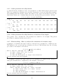
14. April 2012
• Several \newline added to prevent codes from being splitted over two pages
NOTE: This should only be a temporary solution.
Possibilities to prevent latex from splitting the code on two pages:
lstlisting environment options ([float=ht]): The main problem is that the code is
embedded in a float environment but with a fixed starting point. This fixed starting
point can be deleted by the option \begin{lstlisting}[float=ht]. This will hold
the code on one page, but also shift the code somewhere (e.g. code 6 appears before
code 5; code 15 is shifted to the end of file). This decreases readability a lot. Codes
that are naturally longer than one page have to be splitted by hand into two different
listing environments.
\minipage: requires a complete new environment definition with the possible loss of
caption information and unexpected behaviour.
\newpage: Introduce white space and needs to be rechecked after every change of the
document. Codes that are naturally longer than one page have to be splitted by hand
into two different listing environments.
• Changed basicstyle=\footnotesize to basicstyle=\ttfamily in the header of the
LATEXdocument (option of \lstset) to avoid overlapping of symbols in code examples
(e.g. % and M in the Gaussian input header).
13. April 2012
• In subsubsection ”German supercomputer JUROPA” JUROPA runscript added
• In section ”Running Gromacs” flaggs added: -multi, -multidir
• In section ”Plotting, fitting and statistical analysis” subsection ”General comments on
figures” added
• In subsection ”Plotting data” subsubsection ”Grace (Xmgrace)” added
• In subsection ”Gromacs tools” subsubsection ”Order parameter for alkyl chains” added
• In subsection ”Gromacs tools” subsubsection ”Order parameter for alkyl chains as a
function of box length” added
• In subsection ”Gromacs tools” subsubsection ”2D number density map” added
• In subsection ”Gromacs tools” subsubsection ”Head stacking - How to analyse the orientation of aromatic rings” added
• http://www.mathworks.com/matlabcentral/fileexchange/13812and http://web.cecs.
pdx.edu/~gerry/MATLAB/plotting/loadingPlotData.htmladded as useful Matlab scripts
5
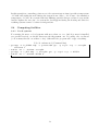
1
System preparation
For all substances under study initial coordinates (*.xyz) and gromacs topology files (*.itp
and * AtTy.itp) are stored in the subfolder “ForceFields“. In addition a Collection of GROMACS topologies for small organic molecules developed and maintained by David van der
Spoel (Sweden) and Carl Caleman (Germany) can be found at http://virtualchemistry.
org/BENCH/and GROMACS user contribution for topologies at http://www.gromacs.org/
Downloads/User_contributions/Molecule_topologies.
1.1
1.1.1
Configurations
Generation of first coordinates
Initial configurations of single wall carbon nanotubes (CNT) can be generated using the online
tool TubeGen1 . It demands the input of chirality and number of replications and generates
for example a .pdb file with the resulting structure.
Nanocarbon onions can be modelled as a collection of carbon fullerenes of different size, e.g.
C720, C320, C60. The coordinates of these substructures can be obtained through databases
like the Fullerene Library by M. Yoshida or special tools like the Nanotube Modeler2 .
Graphene layers can be again prepared in several ways. One version is the use of
ase.structure3 , a tool of the Atomic Simulation Environment (ASE), that is the common
part of the simulation tools developed at CAMd. ASE provides Python modules for manipulating atoms, analyzing simulations, visualization etc.
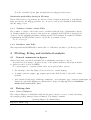
Code 1: graphenesheet.py (Python)
1
2
3
4
5
6
7
8
9
from ase import *
from ase . structure import graphene_nanoribbon
gnr1 = graphene_nanoribbon (3 , 4 , type = ’ armchair ’ , sheet = True )
cell = gnr1 . get_cell ()
print cell
posx = cell [0][0]
posy = cell [1][1]
posz = cell [2][2]
io . write ( ’ g r a p h e n e _ n a n o r i b b o n _ 3 _ 4 _ a r m c h a i r . pdb ’ , gnr1 )
The resulting .pdb file can be transformed, rotated etc. using editconf.
1
Code 2: editconf (Command line)
editconf -s g r a p h e n e _ n a n o r i b b o n _ 3 _ 4 _ a r m c h a i r . pdb - translate 0 0
0 - rotate 0 0 0 -o confout_trans_rot . gro
N-methyl-2-pyrrolidone (NMP), acetonitrile (AN) as well as tetraethylammonium (TEA),
tetrabutylammonium (TBA) and imidazole based ionic liquids like 1-ethyl(butyl,octyl)-3methylimidazolium (EMIm,BMIm,OMIm) with the anions Cl, tetrafluoroborate (BF4) and
bis(trifluoromethylsulfonyl)imide (TFSI) have been modelled using the OPLS-AA force field.
1
http://turin.nss.udel.edu/research/tubegenonline.html
http://www.ccp14.ac.uk/ccp/web-mirrors/jcrystal/products/wincnt/
3
https://wiki.fysik.dtu.dk/ase/epydoc/ase.structure-module.html
2
6
The inital configuration were taken from databases or self prepared with the help of SCHRÖDINGER Maestro software [1].
1
Code 3: Starting Maestro (Command line)
$SCHRODINGER / maestro - SGL
1.1.2
Combining them all to full systems under study
If the coordination files (*.xyz, *.pdb or *.gro) of all single compounds of the system under
study have been created, the preparation of the complete simulation box is straightforward.
It can be done by either using the gromacs tools like genbox4 or by using the free software
PACKMOL [2]. Using genbox would look like
1
Code 4: genbox (Command line)
genbox - cp graphene_sheets . gro - cs C6mimBF4 . gro - maxsol 1240
with having a predefined configuration of two graphene sheets graphene_sheets.gro and a
file with a preequilibrated simulationbox of neat solvent C6mimBF4.gro. Due to the packing
mechanism - placing the whole bulk in the empty space and removing all overlapping molecules
- this method demands time, computational effort and has no safety that it really works. It
is NOT recommended.
The most convinient way to produce a working simulation box is to use PACKMOL [2],
which uses a mathematic / geometric filling algorithm rather than an overlapping test of hard
spheres.
Packmol creates an initial point for molecular dynamics simulations by packing
molecules in defined regions of space. The packing guarantees that short range
repulsive interactions do not disrupt the simulations. The great variety of types
of spatial constraints that can be attributed to the molecules, or atoms within the
molecules, makes it easy to create ordered systems, such as lamellar, spherical or
tubular lipid layers. The user must provide only the coordinates of one molecule
of each type, the number of molecules of each type and the spatial constraints
that each type of molecule must satisfy.5
4
5
http://www.gromacs.org/Documentation/How-tos/Mixed_Solvents
http://www.ime.unicamp.br/~martinez/packmol/
7
A working packmol input would look like:
Code 5: packmol impurity.inp (ASCII file)
1
2
3
4
5
tolerance 2.0
filetype pdb
output packmol . pdb
seed seednum
add_box_sides
6
7
8
9
10
structure top / All_itp / Cation . pdb
number 200
inside box 0. 0. 0. 50.0 50.0 50.0
end structure
11
12
13
14
15
structure top / All_itp / Anion . pdb
number 200
inside box 0. 0. 0. 50.0 50.0 50.0
end structure
16
17
18
19
20
structure top / All_itp / Impurity . pdb
number numberofmol
inside box 0. 0. 0. 50.0 50.0 50.0
end structure
A second script was prepared for changing the name of Cation, Anion and Impurity as
well as the number of impurity molecules, the box size and the seed number for generating
independent replicas of the system using the stream editor sed. Seed numbers that have been
tested so far are 191917, 171719, 151517, 191317, 111719. Any large primary number should
do the job as well.
Code 6: sed (Command line)
1
2
3
4
5
6
7
sed ’s /50.0/ ’ $Box ’/ g ;
s / Impurity / ’ $Imp ’/;
s / numberofmol / ’ $numImp ’/;
s / Cation / ’ $Cation ’/;
s / Anion / ’ $Anion ’/;
s / seednum / ’ $seed ’/ ’
packmol_impurity . inp > packmol_tmp . inp
The final steps are starting PACKMOL and after a successful run the transformation of
packmols output .pdb file to the gromacs input file .gro with the help of editconf6 .
1
2
Code 7: Starting Packmol (Command line)
$HOME / Programs / packmol / packmol < packmol_tmp . inp
editconf -f packmol . pdb -o packmol . gro
6
http://manual.gromacs.org/current/online/editconf.html
8
1.2
1.2.1
Force fields
Carbon nanoparticles
The generation of the force field for carbon nanoparticles is described in detail in Andrey Frolovs tutorial on simulating carbon nanotubes (CNTs) Tutorials/Tutorial_simulate_CNT.
Non-bonded interaction parameters for the nanotube/nanoonion/graphene carbon atoms correspond to the benzene OPLS-AA (all-atom optimized molecular potential for liquid simulation) carbon (opls 145 in Gromacs notation). This was done by using the Gromacs tool
x2top.7
1
Code 8: x2top (Command line)
x2top -f CNT . gro -o CNT . top - name C60 - kb 392459.2 - kt 527.184 pbc
The flagg -name renames the molecule, default is ICE. In the case of periodic carbon nanotubes
and graphene sheets it is very important to add the flagg -pbc, to assure that bonds between
all particles are recognized.
Be aware: the file ffoplsaa.n2t (Gromacs version 3.x) or atomname2type.n2t (Gromacs
version 4.x) needs an aditional line for recognizing all carbon bond. The following two lines
are already included:
1
2
C
C
opls_145
opls_145
Code 9: atomname2type.n2t (ASCII file)
-0.12 12.011 3
C 0.150
C 0.150
-0.12 12.011 3
C 0.133
C 0.150
H 0.108
O 0.140
and should be extended by the last two lines of the following piece:
1
2
3
4
C
C
C
C
opls_145
opls_145
opls_145
opls_145
Code 10: atomname2type.n2t new (ASCII file)
-0.12 12.011 3
C 0.150
C 0.150
-0.12 12.011 3
C 0.133
C 0.150
0.0
12.011 3
C 0.140
C 0.140
0.0
12.011 2
C 0.140
C 0.140
H 0.108
O 0.140
C 0.140
The positions of CNT atoms are restrained to the initial values by harmonic potential
with 1000 kJ · mol−1 · nm−2 force constant in each direction. For restraining the positions of
the carbon atoms the Gromacs tool genrestr can be used. It generates an .itp file that has
to be included in the general topology file of the nanocarbon molecule.
1.2.2
Organic molecules
In the upper section it was mentioned that the inital configuration of organic molecules were
taken from databases or self prepared with the help of SCHRÖDINGER Maestro software
9.0.211 [1]. Again this program is used to generate apropriate OPLS-AA parameter. (See
Code 3 on page 7 how to start Maestro.)
After building the molecule (alternatively reading in a coordinate file downloaded from
a database), the next step is to create a .cms file with system coordinates and force field
applied. This is done by using the menu Applications → Desmond → System Builder. In
7
A nice tutorial as given here: http://chembytes.wikidot.com/gromacs-wiki.
9
the window that pops up the solvent model should be none, all other entries can be set as
default. No ions should be added. Now press start.
The resulting desmond setup-out.cms file can be then transfered to Gromacs files by using
the script Maestro2gmx.py. To do: Usage of the script.
Experience showed that it is very convenient to store all topologies (.itp files) in an own
directory and separate atomtypes with mass, charge and non-bonded interaction parameter
(Lennard-Jones form)
Code 11: BF4 AtTy.itp (ASCII file)
1
2
3
4
[ atomtypes ]
; type
mass
B
10.811
F
18.998
charge
0.8276
-0.4569
ptype sigma
A 3.5814 e -01
A 3.1181 e -01
epsilon
3.9748 e -01
2.5104 e -01
and bonded interation parmeter (in case of inconsistency the upper charges in * AtTy.itp are
used).
Code 12: BF4.itp (ASCII file)
1
2
3
4
5
6
7
8
9
10
11
12
13
14
15
16
17
18
19
20
21
22
23
24
[ moleculetype ]
; name nrexcl
BF4
3
[ atoms ]
;
nr type
resnr
residu atom
cgnr
charge mass
1
B
1
BF4
B
1
0.8276
10.811
2
F
1
BF4
F
1
-0.4569
18.998
3
F
1
BF4
F
1
-0.4569
18.998
4
F
1
BF4
F
1
-0.4569
18.998
5
F
1
BF4
F
1
-0.4569
18.998
[ bonds ]
; ai aj funct
c0
c1
1
2
1
0.137 284512.000
1
3
1
0.137 284512.000
1
4
1
0.137 284512.000
1
5
1
0.137 284512.000
[ angles ]
; ai
aj
ak
funct
c0
c1
3
1
2
1
110.611
502.080
4
1
2
1
110.611
502.080
4
1
3
1
110.611
502.080
5
1
2
1
110.611
502.080
5
1
3
1
110.611
502.080
5
1
4
1
110.611
502.080
The simulation directory should contain then a .top file where all necessary (or even more)
.itp files are included.
10
Code 13: topol.top (ASCII file)
1
2
3
4
5
6
7
8
9
10
11
12
13
14
15
16
17
18
19
20
21
22
23
24
25
26
27
28
# define _FF_OPLS
# define _FF_OPLSAA
[ defaults ]
; nbfunc comb - rule gen - pairs fudgeLJ fudgeQQ
1
3
yes
0.5 0.5
;;; LOAD ATOM TYPES
# include " path / top / EMI_AtTy_lopes . itp "
# include " path / top / BMI_AtTy_lopes . itp "
# include " path / top / OMI_AtTy_lopes . itp "
# include " path / top / Cl_AtTy . itp "
# include " path / top / BF4_AtTy . itp "
# include " path / top / TFSI_AtTy_lopes . itp "
;;; LOAD OPLS FF
# include " localgromacspath / share / gromacs / top / oplsaa . ff /
ffnonbonded . itp "
# include " localgromacspath / share / gromacs / top / oplsaa . ff / ffbonded .
itp "
;;; LOAD MOLECULES *. itp
# include " path / top / EMI_lopes . itp "
# include " path / top / BMI_lopes . itp "
# include " path / top / OMI_lopes . itp "
# include " path / top / Cl . itp "
# include " path / top / BF4 . itp "
# include " path / top / TFSI_lopes . itp "
[ system ]
; Name
Neat BMI BF4
[ molecules ]
BMI 200
BF4 200
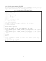
1.2.3
Charges
In the case of organic molecules the OPLS-AA forcefield has proved to give reasonable results
in many cases. But it might be a good idea to play with the charges. With Gaussian03 [3]
charges can be calculated based on quantum mechanics. An input file .com for calculating
charges of a molecule would look like
Code 14: Head of Gaussian input .com (ASCII file)
1
2
3
4
% Nprocshared =4
% Mem =1 GB
% Chk = scna_HF_6 -31 Gd . chk
# p hf /6 -31 g ( d ) nosymm geom = connectivity pop = chelpg
with the addition of particle positions and bond information.
11
2
2.1
Running simulations with Gromacs
Molecular dynamics parameter file .mdp
After creating / preparing the coordinate and topology files the only missing files are the
.mdp files which define the simulation parameter, like integrator, annealing proceadure, temperature, etc. A sample file is given here:
1
2
3
4
5
6
7
8
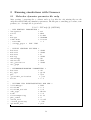
Code 15: NPT.mdp (1) (ASCII file)
; RUN CONTROL PARAMETERS =
integrator
= md
tinit
= 000
dt
= 0.002
nsteps
= 500000
comm - mode
= Linear
; nstcomm
= 1
; energy_grps = EMI TFSI
9
10
11
12
13
14
15
16
17
18
; OUTPUT CONTROL OPTIONS =
nstxout
= 1000
nstvout
= 1000
nstfout
= 0
nstlog
= 1000
nstenergy
= 50
nstxtcout
= 500
xtc_precision
= 1000
xtc_grps
=
19
20
21
22
23
24
25
; NEIGHBORSEARCHING PARAMETERS =
nstlist
= 10
ns_type
= grid
pbc
= xyz
; periodic_molecules
= yes
rlist
= 1.3
26
27
28
29
30
31
32
33
34
35
36
37
; OPTIONS FOR ELECTROSTATICS AND VDW =
coulombtype
= PME
rcoulomb
= 1.3
rcoulomb_switch
= 1.0
vdw_type
= Shift
rvdw
= 1.0
fourierspacing
= 0.12
pme_order
= 4
ewald_rtol
= 1e -05
; ewald_geometry
= 3 dc
optimize_fft
= yes
12
1
2
3
4
5
6
7
8
9
10
11
12
13
14
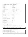
Code 16: NPT.mdp (2) (ASCII
; OPTIONS FOR WEAK COUPLING ALGORITHMS =
tcoupl
= v - rescale
tc - grps
= System
tau_t
= 1.0
ref_t
= 298.1
Pcoupl
= Berendsen
Pcoupltype
= isotropic
tau_p
= 1.0
compressibility
= 4.5 e -5 ; 1e -5
ref_p
= 1.0
; bar
; Pcoupltype
= semiisotropic
; tau_p
= 1.0 1.0
; compressibility
= 4.5 e -5 0.0 ;
; ref_p
= 1.0
1.0 ;
file)
0 0 0
1e -5 0 0 0
bar
15
16
17
18
19
; GENERATE VELOCITIES FOR STARTUP RUN =
gen_vel
= yes
gen_temp
= 298.1
gen_seed
= 473529
20
21
22
23
24
25
26
27
28
29
; OPTIONS FOR BONDS
constraints
constraint_algorithm
unconstrained_start
shake_tol
lincs_order
lincs_warnangle
morse
lincs_iter
2.2
=
=
=
=
=
=
=
=
=
hbonds
lincs
no
0.00001
4
30
no
2
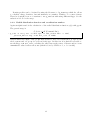
Running Gromacs
In general it is necessary to produce a run input file for Gromacs first. This is done by the
tool grompp, which also helps detecting numerous input errors.
1
Code 17: grompp (Command line)
grompp -f 1 _NPT . mdp -c steep . gro -p topol . top -o NPT
Then the molecular dynamics run can be started with mdrun.
1
2
3
4
Code 18: mdrun (Command line)
mdrun - deffnm NPT - maxh 1
mdrun - deffnm NPT - maxh 1 - cpi NPT . cpt - append
mdrun - deffnm NPT - maxh 1 - multi 4
mdrun - deffnm NPT - maxh 1 - cpi NPT . cpt - append - multidir $path1
$path2 $path3 $path4
13
The flagg -deffnm saves all files under the given name but with proper extension NPT.log,
NPT.trr, NPT.xtc and so on. This is especially useful when starting in the same folder several
simulations like steep, NPT and NVT. The flagg -maxh t stops Gromacs after 0.99 · t hours
while writing a checkpointfile for the last step. The second line shows how to continue the simulation using the checkpoint file with -cpi NPT.cpt and appending the new output to the old
files using -append. Two usefull flaggs -multi n and -multidir $path1 $path2 $path3 $path4
with the same goal are introduced in line 3 and 4 of the above starting lines for mdrun. Gromacs
allows to summarize several independend simulations into one job - allowing even for small
systems the usage of super computers. 8 In case of -multi n n .tpr files have to be stored in
one folder being numbered as follows: NAME0.tpr, NAME1.tpr, NAME2.tpr, NAME3.tpr, ... The
flagg -multidir $path1 $path2 $path3 $path4 was introduced in Gromacs version 4.5.4,
unfortuantely an entry in the general help mdrun -h is still missing. With -multidir .tpr
files can be stored in differend folders $path*, but should all have the same name NAME.tpr.
It depends on the personell preferences which of these two options to use.
2.2.1
Energy minimization and equilibration
The first step after system preparation should be a basic energy minimization to remove
high forces that would lead to a system explosion. In Gromacs this is done by changing the
integrator to steep in the .mdp file using integrator = steep.
The number of steps can range between 1000 and several 10000. If the initial configuration
was created with Packmol and the initial density was reasonable, only a few minimization
steps are sufficient to relax the system and start molecular dynamics simulations. If a bigger
number of minimization steps is necessary, it also might be better to do energy minimizations
of 1000 steps and redo the proceadure with the resulting configuration several times.
Andrey Frolov figured out while working on energy minimization, that it is not sufficient to
run Gromacs in single precision to obtain reasonable results. Convergence of the energy is in
most cases only reached when using Gromacs in double precision (this is done by recompiling
the source code).
For system equilibration NPT simulations should be performed. In cases of low viscous fluids it takes a few 10 ps until the density reaches a constant value. In case of room-temperature
ionic liquids it might be necessary to equilibrate at least 1 ns.
2.2.2
Production runs
A production run means a molecular dynamics simulation run that is resulting in enough data
to sample the ensemble space correctly and that allows statistical reliable analysis of data.
The length of a production run depends on the system size (the more molecules are included
in the simulation box the highter is the probability so sample all configurations within a given
time frame). The length also depends on the viscosity of a system (or how fast particles are
moving, equal to how fast they forget about theirs past).
The systems under study in our group demanded for simulation lenghts between 30 ns and
100 ns.
One option to ensure sufficient data is the usage of replica runs as explained in Section
2.3 on page 15.
8
Gromacs shows reasonable parallelization if not less than 1000 atoms per core are used. Below 500 atoms
per core the simulations are liable to crash. These limits are due to network comunication.
14
2.2.3
Data storage for further analysis
In case of water simulations a rule of thumb tells to sample coordinates each 0.3 ps. In
case of room-temperature ionic liquids 1 ps seems already sufficient and might be due to
the slow dynamics increased even more if disc space is an issue. For analysis of velocity
autocorrelation function and ionic conductivity the velocities of the system should be sampled
each 40 fs = 0.04 ps (according to Maginn, for 4 ns), be cautious, this fast results in several
GB of disk space needed per simulation.
2.3
Running replicas
There are three possibile ways to get a set of independet system configurations (replicas) for
improving analysis quality and covering the whole thermodynamic ensemble.
2.3.1
Independent initial configurations by different random seeds
Preparation of independent initial configurations by using different seeds with Packmol. Seed
numbers that have been tested so far are 191917, 171719, 151517, 191317, 111719. Any large
primary number should do the job as well.
2.3.2
Grabbing frames from a trajectory
For simulating replicas it might be useful to take the first sucessful production run and only
grep a few configurations out of it. While assigning random velocities and / or additional
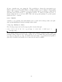
heating in many cases the configurations can be taken as independant. The following script
takes the .xtc files from a directory called ”anneal”. Then it greps coordinate files out of
these .trr files using the Gromacs tool trjconv. The resulting frames are stored with the given
name "$name"_rep.gro plus a running number, e.g. "$name"_rep0.gro, "$name"_rep1.gro,
"$name"_rep2.gro, etc.
Code 19: grepreplicas.sh (Bash script)
1
2
3
4
5
# !/ bin / bash
for itrr in ’ ls ./ anneal /*. xtc ’; do
name = ’ echo $itrr | sed " s /. xtc // g " ’
echo 0$ ’\ n ’ q | trjconv -s " $name " . tpr -f " $name " . xtc -o "
$name " _rep . gro - sep -b 120 - dt 50
done
2.3.3
System heating
After the preparation of one coordinate file it is possible to heat the system using the annealing
algorithm.
1
2
3
4
annealing
annealing_npoints
annealing_time
annealing_temp
Code 20: annealing (ASCII file)
= single
= 2
= 0 1000
= 1500 350
15
In this example two annealing points are set, the system starts at time 0 ps with a temperature
of 1500 K and within the next 1000 ps the system is smoothly cooled down to the simulation
temperature of 350 K. In a system with fast diffusing particles this proceadure is very useful,
but the highter the viscosity of a system the less happens during the heating and therefore
resulting systems cannot be taken as independent.
2.4
2.4.1
Computing facilities
Local systems
For starting Gromacs on local systems with more than one core (and if gromacs is installed
as a parallel version) one should always use the flagg mdrun -nt 1 for using only one thread
(or how many threads one wishes to use). Otherwise the program will occupy everything.
1
2
3
4
grompp -f
maxwarn
mdrun - nt
grompp -f
mdrun - nt
Code 21: mdrun -nt 1 (Command line)
0 _STEEP . mdp -c packmol$k . gro -p topol . top -o steep$k 1
1 - deffnm steep$k
1 _NPT . mdp -c steep$k . gro -p topol . top -o NPT$k
1 - deffnm NPT$k &
16
2.4.2
British supercomputer HECToR
For running simulations on the British supercomputer HECToR the following start script
might be useful (submitted using qsub runscript_parallel.pbs):
1
2
3
4
5
6
7
8
9
Code 22: runscript parallel.pbs (Bash script)
# !/ bin / bash -- login
# PBS -N NAME
# PBS -q parallel
# PBS -l mppwidth =24
# PBS -l mppnppn =24
# PBS -A x01 - fedo
# PBS -V
# PBS -l walltime =01:00:00
# -l cput =00:05:00
10
11
12
13
echo $PBS_O_WORKDIR
# Shift to the directory we submitted the job from
cd $PBS_O_WORKDIR
14
15
module add xe - gromacs
16
17
18
19
# Get the number of MPI tasks and tasks per node
export NPROC = ‘ qstat -f $PBS_JOBID | grep mppwidth | awk ’{ print
$3 } ’ ‘
export NTASK = ‘ qstat -f $PBS_JOBID | grep mppnppn | awk ’{ print
$3 } ’ ‘
20
21
22
tpr = NPT
MAXH =1
23
24
25
aprun -n $NPROC -N $NTASK mdrun_mpi - maxh $MAXH - deffnm $tpr dlb auto
# - cpi state . cpt - append
17
Analysis (e.g. g rdf) can be done in serial using the following submission script:
1
2
3
4
5
6
Code 23: runscript serial.pbs (Bash script)
# !/ bin / bash -- login
# PBS -N NAME
# PBS -q serial
# PBS -A x01 - fedo
# PBS -V
# PBS -l cput =01:00:00
7
8
9
10
echo $PBS_O_WORKDIR
# Shift to the directory we submitted the job from
cd $PBS_O_WORKDIR
11
12
13
14
# Load the CASTEP module
# module add xe - gromacs
./ run_msd . sh
with run msd.sh:
Code 24: run msd.sh (Bash script)
1
2
3
4
5
6
7
8
9
# !/ bin / bash
for i in ‘ ls -d EMI */ ‘ ; do
cd $i
echo Cation |
g_msd -f traj . xtc -s NVT . tpr -n rdf_index . ndx -o msd_Cation .
xvg -b 4000
echo Anion |
g_msd -f traj . xtc -s NVT . tpr -n rdf_index . ndx -o msd_Anion . xvg
-b 4000
cd ..
done
18
2.4.3
German supercomputer JUROPA
For running simulations on the German supercomputer JUROPA the following start script
might be useful (submitted using msub runscript_JUROPA):
Code 25: runscript JUROPA.pbs (Bash script)
1
2
3
4
# !/ bin / bash
# MSUB -l nodes =1: ppn =8
# MSUB -l walltime =24:00:00
# MSUB -v tpt =1
5
6
7
module load gromacs /4.5.5
module load mkl /10.2.5.035
8
9
10
# Prepare the Gromacs run
# grompp -f NVT . mdp -c packmol . gro -p topol . top -n index . ndx -o
NVT
11
12
13
# Run the MD on 8 cores
mpiexec - np 8 -- exports GMXLIB $GROMACS_ROOT / bin / mdrun_d - deffnm
NVT - maxh 24
Further details can be obtained from the JUROPA webpage with quick introductions
http://www.fz-juelich.de/ias/jsc/EN/Expertise/Supercomputers/JUROPA/UserInfo/
QuickIntroduction.html.
2.5
Comments
• When running simulations with periodic molecules it is very important to include in the
.mdp file the line
1
periodic_molecules = yes
otherwise e.g. graphene sheets will form a ball ...
• For slab geometries
1
ewald_geometry = 3 dc
should be added, but this line has to be avoided when doing bulk simulations. The
simulations may either crash or show weired physical behaviour such as formation on
vacuum bubbles or continous increasing and decreasing of volume (“breathing”).
• On some computers simulations are crashing due to some error using PME dynamic load
balancing. Therefore by using the option mdrun -dlb no the dynamic load balancing
can be switched off and systems may run more stable.
19
3
3.1
System analysis
Visual analysis
The program of choice for looking at trajectories is Visual Molecular Dynamics (VMD) [4].
It is useful to read in a trajectory, track special particles (atoms, molecules, residues etc) and
prepare nice pictures of the molecular systems. They provide also analysis tools for example of
radial distribution functions or mean square deviation from an input structure, but if possible
it is preferable to use GROMACs tools or self written scripts.
A Gromacs trajectory can be read in via the terminal by using the following command
(this is much more preferable than reading in a trajectory using the gui, for the trajectory is
not displayed and therefore reading in is much faster).
1
Code 26: Start VMD (Command line)
vmd - gro test . gro - xtc test . xtc
The box boundaries can be shown using Extensions → Tk Console and typing in
pbc box.
To do: Add some useful lines for particle selection.
3.2
Gromacs tools
One reason for the wide acceptance and usage of Gromacs is the enormous number of analysis
tools that are provided by the developer and which can be found at http://www.gromacs.
org/Documentation/Gromacs_Utilities. They are all preinstalled and can be started just
by using the command line as it is possible for grompp or mdrun.
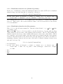
3.2.1
Density and density profile
The first look that should be taken after a simulation finished sucessfully (and also if not)
is how temperature, energy, volume etc evolved over time. This can be done straightfoward
using the tool g_energy.
Code 27: g energy (Bash script)
1
2
3
4
5
6
7
8
9
10
# !/ bin / bash
for Cation in EMI BMI OMI ; do
for Anion in Cl BF4 TFSI ; do
cd Bulk_neat / $Cation \ _$Anion
for k in 0 1 2; do
echo 7 8 9 10 11 16 17 | g_energy -f ener$k . edr -s NPT$k . tpr -o
$Cation \ _$Anion \ _$k . xvg
done
cd ../../
done
done
The resulting .xvg files can be read in by numerous programs, e.g. Gnuplot, Matlab,
Grace, and analyzed further (e.g. plotted, statistical analysis of mean, std, etc.). See section
4 on page 27.
20
Density profiles can be obtained by using the Gromacs tool g_density, which also allows
to calculate charge densities, but unfortunately not number densities of a center-of-mass.
Therefore it might be more convenient to use g_rdf but with using different flaggs. See the
subsection below for the usage.
3.2.2
Radial distribution function and coordination number
Again straightforward is the calculation of the radial distribution function g(r) with g_rdf.
The general usage is
1
Code 28: g rdf (Command line)
g_rdf -f traj . xtc -s NPT . tpr -n rdf_index . ndx -o rdf \
_Cation_Anion . xvg - rdf mol_com -b 2000
with an interactive input of the groups that should be used. By default these groups are the
whole system and one group for every molecule type. In this case it is phsical reasonable to
use the flagg -rdf mol_com to calculate the rdfs between the center of masses and not some
cummulative value between all atoms (which is done by VMD’s tool, so be careful).
21
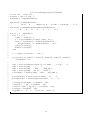
If the task is to analyse rdfs between certain atoms, it is necessary to use new groups by
creating a customized index file which is done by the Gromacs tool make_ndx.
Code 29: make ndx non-interactive (Bash script)
1
2
3
4
5
6
7
8
9
10
11
12
13
14
15
16
17
18
19
# !/ bin / bash
make_ndx -f confout0 . gro
keep 0
ri 1 -200
name 1 Cation
ri 201 -400
name 2 Anion
a OW | a HW1 | a HW2
name 3 SOL
a N1a1 | a N1b1 | a C4a1
a N1a3 | a N1b3 | a C4a3
a N1a4 | a N1b4 | a C4a4
name 4 Head
a C1b1
a C1d3
a C1d4
name 5 Tail
q
EOF
-o rdf_index . ndx << EOF
| a C4b1 | a C4c1 |
| a C4b3 | a C4c3 |
| a C4b4 | a C4c4 |
With the given index file g_rdf can be used again, this time without interactive usage
but rather within a shell script. Notice the usage of group names instead of numbers, which
makes the usage of g_rdf less prone to error and reusable if the system structure changes.
Code 30: g rdf non-interactive (Bash script)
1
2
3
# !/ bin / bash
for k in 0 1 2
do
4
5
6
7
8
g_rdf -f traj$k . xtc -s NPT$k . tpr -n rdf_index . ndx -o rdf$k \
_Cation_Anion . xvg - rdf mol_com -b 2000 << EOF
Cation
Anion
EOF
9
10
11
12
13
g_rdf -f traj$k . xtc -s NPT$k . tpr -n rdf_index . ndx -o rdf$k \
_Cation_SOL . xvg - rdf mol_com -b 2000 << EOF
Head
SOL
EOF
14
15
done
22
3.2.3
Distribution function in cylindrical geometry
In the case of cylindrical geometry the distribution function around a CNT can be calculated
using the flagg -xy if the nanotube is oriented in z direction.
1
Code 31: rdp.sh (Command line)
g_rdf - bin $bin -b $begin -e $end -f " $run " . xtc -s " $run " . tpr -n
index . ndx -o $fname - cn cn_ " $fname " - rdf mol_com - xy
The resulting rdfs will not go to one in infinite space but rather to a constant value different
from one. This is due to the solvent excluded volume of the CNT and therefore the rdf has
to be renormalized.
3.2.4
Distribution function in slab geometry
Take a look on the Gromacs manual for “Interface-related items”, e.g. g order, g density,
g potential, g traj.
In addition to those tools it is possible to use the Gromacs tool g_rdf with the flagg
-surf, taken the carbon atoms of the graphene wall as reference. The tool will caclulate the
distance between any atom / center-of-mass with respect to the atoms of the surface. This is
not completly correct as the length of the hypotenuse is not identical with the exact distance
between a flat wall and the atom, but in most cases the induced error will be less than 3 %
(assuming a distance between carbon atoms of the wall of 1.4 Åand a distance between atom
and wall of at least 5 Å).
Code 32: dpz.sh (Command line)
1
2
3
4
5
# !/ bin / bash
g_rdf - bin $bin -b $begin -e $end -f " $run " . xtc -s " $run " . tpr -n
index . ndx -o $fn - cn cn_ " $fn " - rdf $rdftype - surf mol - nopbc
<< EOF
$p1
$p2
EOF
23
3.2.5
Order parameter for alkyl chains
g_order allows the calculation of the order parameter for alkyl chains (angle between z-axis
and vector spanned by 3 distinct carbon atoms). Preparation of a proper index file is required,
the resulting index file should contain only entries of the carbon atoms that belong to the
alkyl chain. In the case of imidazolium cations also the first Nitrogen is added to the list.
Code 33: index order.ndx (ASCII file)
1
2
3
4
5
6
[ N0 ]
2
21
249
[ C1 ]
13
32
260
[ C2 ]
9
28
256
3.2.6
40
59
268
78
97
116
135
154
173
192
211
230
51
279
70
89
108
127
146
165
184
203
222
241
47
66
275
85
104
123
142
161
180
199
218
237
Order parameter for alkyl chains as a function of box length
Use g_order -sl to calculate the order parameter as a function of box length. The general
proceadure is explained in the section above.
3.2.7
Head stacking - How to analyse the orientation of aromatic rings
g_sgangle -z calculates the angle between z-axis and vector spanned by 3 defined atoms.
Unfortunately only one molecule per calculation is allowed. This will introduce the following
procedure for an analysis of all cations:
1
2
3
4
5
Code 34: g sgangle -z (workflow)
While ( Browse through all cations )
do Make index file for cation
do Run g_sgangle -z
do Sum up histogram of angle distribution
Print normalized histogram
g_sgangle calculates the angle between 2 vector spanned by 6 defined atoms: The procedure gets somewhat more complicated for the analysis of all cations:
1
2
3
4
5
6
7
Code 35: g sgangle (workflow)
While ( Browse through all cations )
do Make index file for cation
While ( Browse through all other cations )
do Make index file for other cation
do Run g_sgangle
do Sum up histogram of angle distribution
Print normalized histogram
24
3.2.8
2D number density map
An interesting tool for visualizing number density distribution is g_densmap. Check carefully
the range that is taken into account when analysing interfaces.
1
2
Code 36: g densmap (Command line)
g_densmap -f NVT . xtc -s NVT . tpr - aver z - xmin 1.65 - xmax 2.15 -b
4000 -e 10000
convert densmap . xpm densmap . eps
3.3
3.3.1
Self written scripts
Potential of mean force and free energy
The calculation of the potential of mean force (PMF) can easily be done by using any mathematical programming language (e.g. Matlab, FORTRAN), taking the initial obtained radial
distribution functions and calculating
P M F (r) = −kB · T · ln(g(r)).
The PMF can be used to estimate the free energy of the process of dividing one water
molecule from a full solvated ion by calculating the depth of the first minimum of the ion-water
PMF.
3.3.2
Orientation analysis
The Gromacs tool g_sorient analyzes solvent orientation around solutes. It calculates two
angles between the vector from one or more reference positions to the first atom of each
solvent molecule (the angle between a vector spanned by 3 defined atoms (A1, A2, A3) and
the vector spanned by another atom (B1) plus the first atom of the predefined atoms (A1)).
Therefore the atoms of the solvent to use have to be specified using an index file. On the
preparation of index files see Code 29 on page 22.
Modified version of g sorient for cylindrical geometry
Orientation distributions are calculated with the g_sorient which has to be modified to
be able to handle cylindrical symmetry of CNTs and to be able to resolve the orientation
probability density as a function of distance.
The usage is the following:
1
Code 37: g sorient (Command line)
g_sorient -f run1 . xtc -s run1 . tpr -n index . ndx -o sori_OMI_COM .
xvg - ro sord_OMI_COM . xvg - xy - com -b 2000 -e 32000 - rmax 3.0
- nat2 37 - ati21 13 - ati22 9 - ati2cen 1 - rbin 0.01 - cbin 0.1
The distributions of cos(θ1 ) for rmin ≤ r ≤ rmax are calculated with respect to the center-ofmass of the solvent molecules (-com) and along the z-axis (-xy). The following list describes
all additional options implemented by Andrey Frolov:
25
1
{
2
{
3
{
4
{
5
{
6
{
7
{
g sorient.c flaggs (C)
" - nat1 " , FALSE , etINT , {& nat1 } , " Number of atoms in the
reference molecules " } ,
" - nat2 " , FALSE , etINT , {& nat2 } , " Number of atoms in the
molecules to calculate orientation " } ,
" - ati11 " , FALSE , etINT , {& ati11 } , "( Vector origin ) Atom
index on reference molecule " } ,
" - ati12 " , FALSE , etINT , {& ati12 } , "( Vector end ) Atom index
on reference molecule " } ,
" - ati21 " , FALSE , etINT , {& ati21 } , "( Vector origin ) Atom
index on molecule to calculate orientation " } ,
" - ati22 " , FALSE , etINT , {& ati22 } , "( Vector end ) Atom index
on molecule to calculate orientation " } ,
" - ati2cen " , FALSE , etINT , {& ati2cen } , "( Vector end ) Atom
index on molecule to calculate orientation " } ,
The following description of the analysis routine was taken from Andrey Frolov’s PhD
thesis.
We calculated the average number of particles at a certain distance r around CNT
in the following way:
n∆r=0.01 nm (r) = ρ0 ·
ρ(r)
· 2πr · ∆r
ρ0
is the RDP of
where ρ0 is the bulk density of the corresponding particles, ρ(r)
ρ0
the corresponding particles, n∆r=0.01 nm (r) is the average number of particles at a
certain distance r in the cylindrical volume segment with the difference between
radii of smaller and larger cylinders of ∆r.
To use the modified Gromacs script, it is necessary to recompile the complete source code.
That means, the follwing steps have to be done:
• Compile the Gromacs code on a local folder.
1
2
Code 38: Compiling Gromacs (Command line)
./ configure -- prefix =[ your gmx folder ]
make
• Copy the gmx_sorient.c to the [your gmx folder]/src/tools/ folder and remove
the old files.
1
Removing old files (Command line)
rm g_sorient g_sorient . o
• Recompile Gromacs.
1
2
Recompiling Gromacs (Command line)
cd [ your gmx folder ]
make
26
Now the executable [your gmx folder]/src/tools/g_sorient is new.
Orientation probability density in 2D maps
The modified version of g_sorient produces a solvent orientation map sord_*.xvg with the
name provided by the flagg g_sorient -ro. It can be read in and visualized using Matlab
and the image object.
3.3.3
Volumes of solute cavities ToDo
The volumes of cavities of molecules can be calculated with the help of Gaussian03 software
[3]. In this example the geometries of the species are optimized at the B3LYP/6-31g(d,p) level
of theory. In the quantum mechanics calculations the Self Consistent Isodensity Polarizable
Continuum Model (SCI-PCM) is used to model the acetonitrile solvent.
To do: add script
3.3.4
Residence time ToDo
Old script written in FORTRAN by Andrey Frolov. Will take some time to get the key points.
4
Plotting, fitting and statistical analysis
4.1
General comments on figures
Always check title, axis labels and units before submitting any figure to anyone.
In general most plotting tools allow storage of the figures in many formats (most handy
is .eps as it can be read in by LATEX).
To convert figures to a specific format, there are in general three options:
1. Use an image editor like Gimp. (Very slow in case of many figures.)
2. A simple convert figure.jpg figure.eps in the shell should do the trick on unix
systems.
3. More advanced is the usage of Inkscape: inkscape --file=figure.jpg --export-eps=figure.e
Numerous options like flipping are explained here: http://tavmjong.free.fr/INKSCAPE/
MANUAL/html/CommandLine.html.
4.2
4.2.1
Plotting data
Grace (Xmgrace)
The software Xmgrace is distributed with the Gromacs software or can be downloaded using
the synaptic package manager (keyword Grace). The simple command
Starting Xmgrace (Command line)
1
Xmgrace NAME . xvg
27
allows to visualize any .xvg output file. The possibilities to change the representation are
limited, therefore plotting with Matlab or Gnuplot might be more handy for high quality
images. The advantage of Xmgrace lies in its fast usage and the possibility to make labels
and units given in the header of .xvg human readable. To make an eps-file use File →
Print setup and choose as device EPS. This only sets up the printing, do get the eps-file
printed use File → Print.
4.2.2
Matlab
A handy tool for plotting data with Matlab can be downloaded at http://web.cecs.pdx.
edu/~gerry/MATLAB/plotting/loadingPlotData.html.
*.xvg (e.g. density vs. time)
The following script reads in all energy.xvg files obtained through
1
echo 7 8 9 10 11 16 17 | g_energy -f ener . edr -s NPT . tpr -o
energy . xvg
in the current directory and plots the column eight (vals{8}, density) versus column one
(vals{1}, time). This is done for three replicas on one goal which have seperate file names
*_a.xvg, *_b.xvg and *_c.xvg. In addition the mean value of a certain part (hopefully a
plateau) is calculated and printed in a format directly usable in LATEX.
28
1
2
3
Code 39: analysingenergy.m (1) (Matlab)
clear all ; close all ;
fnames = dir ( ’ *. xvg ’) ;
numfids = length ( fnames ) ;
4
5
6
7
8
fprintf ( ’ % -30 s %10 s %3 s \ n ’ ,...
’
RTIL
&
Impurity & ’ , ’$ \ rho / kg / m ^3 $ ’ , ’ \\ ’) ;
fprintf ( ’ % -30 s %3 s %10 s %3 s %10 s %3 s %10 s %3 s \ n ’ ,...
’ ’ , ’ & ’ , ’a ’ , ’ & ’ , ’b ’ , ’ & ’ , ’c ’ , ’ \\ ’) ;
9
10
11
12
13
14
15
16
17
18
for K = 1: numfids /3
for J = 1:3
count = 3*( K -1) + J ;
a = fopen ( fnames ( count ) . name , ’ rt ’) ;
vals = textscan (a , ’% f % f % f % f % f % f % f % f ’ ,...
’ Headerlines ’ ,8 , ’ CommentStyle ’ , ’@ ’) ;
time { J }= vals {1};
dens { J }= vals {8};
end
19
20
f = figure ( ’ visible ’ , ’ off ’) ;
21
22
plot ( time {1} , dens {1} , time {2} , dens {2} , time {3} , dens {3} , ’
LineWidth ’ ,3) ;
23
24
25
26
27
28
tmp = strrep ( fnames (3*( K -1) + J ) . name , ’ _c . xvg ’ , ’ ’) ;
tmp = strrep ( tmp , ’_ ’ , ’ ’) ;
tmp = strrep ( tmp , ’ BF4 ’ , ’ BF$_4$ ’) ;
tmp = strrep ( tmp , ’1 M no ’ , ’ neat ’) ;
titlename = strrep ( tmp , ’ SOL ’ , ’ H$_2$O ’) ;
29
30
31
picturename = strrep ( titlename , ’& ’ , ’ ’) ;
picturename = strrep ( picturename , ’$ ’ , ’ ’) ;
32
33
34
35
36
37
title ( picturename , ’ FontSize ’ ,18) ;
xlabel ( ’t / ps ’ , ’ FontSize ’ ,18) ;
ylabel ( ’\ rho / kg / m ^3 ’ , ’ FontSize ’ ,18) ;
set ( gca , ’ FontSize ’ ,18) ;
legend ( ’a ’ , ’b ’ , ’c ’ , ’ Location ’ , ’ Best ’) ;
29
1
2
3
Code 40: analysingenergy.m (2) (Matlab)
savename = strrep ( fnames (3*( K -1) + J ) . name , ’ _2 . xvg ’ , ’. png ’) ;
savename2 = strcat ( ’ path / Figures_density / ’ , savename ) ;
saveas (f , savename2 , ’ png ’) ;
4
5
fclose ( a ) ;
6
7
8
9
10
11
12
13
14
15
16
17
fprintf ( ’ % -30 s %3 s %10.2 f %3 s %10.2 f %3 s %10.2 f %3 s \ n ’ , titlename , ’ &
’ ,...
mean ( dens {1}(2000:10000) ) , ’ & ’ ,...
mean ( dens {2}(2000:10000) ) , ’ & ’ ,...
mean ( dens {3}(2000:10000) ) , ’ \\ ’) ;
tmp =[ mean ( dens {1}(2000:10000) ) ...
mean ( dens {2}(2000:10000) ) mean ( dens {3}(2000:10000) ) ];
meanmean = mean ( tmp ) ;
errormean = std ( tmp ) ;
% fprintf ( ’% -30 s %3 s %10.2 f %3 s %10.1 f %3 s\n ’, titlename ,’ & ’ ,...
meanmean , ’ & ’ , errormean , ’ \\ ’) ;
end
30
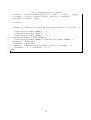
2D maps (e.g. orientation analysis)
Andrey Frolovs scripts for plotting the 2D maps are given here. The script
PlotOrientationIL.m calls the function CF_orient_2D stored in CF_orient_2D.m.
1
2
3
4
5
6
7
8
9
10
11
12
13
14
15
16
17
18
19
20
21
22
23
24
25
26
27
28
Code 41: CF orient 2D.m (Matlab)
function CF_orient_2D (x , phi , cdata1 )
% CREATEFIGURE ( CDATA1 )
% CDATA1 : image cdata
fs =30;
figure1 = figure ( ’ XVisual ’ ,...
’0 x27 ( TrueColor , depth 24 , RGB mask 0 xff0000 0 xff00 0 x00ff )
’) ;
%% figure1 = figure (’ XVisual ’ , ’0 x27 ( TrueColor , depth 24 , RGB
mask 0 xff0000 0 xff00 0 x00ff ) ’);
set ( figure1 , ’ Position ’ ,[300 300 800 600]) ;
axes1 = axes ( ’ Parent ’ , figure1 , ’ LineWidth ’ ,2 , ’ Layer ’ , ’ top ’ ,...
’ FontSize ’ ,fs ,...
’ YTick ’ ,[ -1 -0.5 0 0.5 1] ,...
’ XTick ’ ,[ 0.5 1.0 1.5 1.7 2.0 2.5 ] ,...
’ XMinorTick ’ , ’ on ’ ,...
’ YMinorTick ’ , ’ on ’ ,...
’ TickLength ’ ,[0.02 0.06] ,...
’ CLim ’ ,[0 1]) ;
% Uncomment the following line to preserve the X - limits of the
axes
box ( axes1 , ’ on ’) ;
hold ( axes1 , ’ all ’) ;
% Create image
image ( x , phi , cdata1 , ’ Parent ’ , axes1 , ’ CDataMapping ’ , ’ scaled ’) ;
xlim ( axes1 ,[0.6 1.7]) ;
% Uncomment the following line to preserve the Y - limits of the
axes
ylim ( axes1 ,[ -1 1]) ;
caxis ([0 1.5]) ;
xlabel ( ’r [ nm ] ’ , ’ FontSize ’ , fs ) ;
ylabel ( ’ cos (\ phi ) ’ , ’ FontSize ’ , fs ) ;
colorbar ( ’ peer ’ , axes1 , ’ FontSize ’ , fs ) ;
31
Code 42: PlotOrientationIL.m (Matlab)
1
2
3
4
5
6
7
8
9
10
11
12
13
14
15
16
17
18
19
20
21
22
23
24
25
26
27
28
29
30
31
32
33
34
35
36
37
38
39
40
41
42
43
path ( path , pwd ) ;
cur_dir = pwd ;
x =(0.00:0.01:2.99) ’;
phi =( -0.95:0.1:0.95) ’;
list_dir = {...
’2 M_ACN_EMI_TFSI ’ ,...
’2 M_ACN_BMI_TFSI ’ ,...
’2 M_ACN_OMI_TFSI ’ ,...
’ NEAT_EMI_TFSI ’ ...
};
list_sub_dir = {...
’ q_05 ’ ,...
’ q0 ’ ,...
’ q05 ’ ...
};
mols_list ={...
’ CAT ’ ,...
’ TFSI ’ ...
};
for d =1: length ( list_dir )
for sd =1: length ( list_sub_dir )
for n =1: length ( mols_list )
if strcmp ( list_dir { d } , ’2 M_ACN_BMI_TFSI ’)
mols_list {1}= ’ BMI ’;
elseif strcmp ( list_dir { d } , ’2 M_ACN_OMI_TFSI ’)
mols_list {1}= ’ OMI ’;
else
mols_list {1}= ’ EMI ’;
end
fn = [ ’ sori_ ’ mols_list { n } ’ _COM . dat ’ ];
dfn = [ cur_dir ’/ ’ list_dir { d } ’/ ’ list_sub_dir { sd } ’/ ’ fn
];
arr = load ( dfn ) ;
c = reshape ( arr (: ,3) ,[20 300]) ;
CF_orient_2D (x , phi , c ) ;
xlim ([0.6 1.7]) ;
caxis ([0 1.5]) ;
ofn = [ cur_dir ’/ ’ list_dir { d } ’/ ’ list_sub_dir { sd } ’/ ’
mols_list { n } ’. png ’ ];
ofn ( ofn == ’ - ’) = ’_ ’;
eval ([ ’ print - dpng - r200 ’ ofn ]) ;
close all
end
end ; end ;
exit ;
32
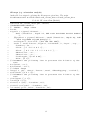
4.3
4.3.1
Fitting data
Matlab
Fitting in Matlab can be done using splines. An amazing code can be downloaded from
Matlabs file exchange http://www.mathworks.com/matlabcentral/fileexchange/13812.
It is called splinefit and smoothes even the noisiest data set.
4.4
Statistical analysis ToDo
4.4.1
Matlab
4.4.2
R
5
How does your system look like when ...
As force fields are only model approaches of real systems, they may not cover the correct
physical behaviour in all imaginable circumstances. The formation of crystals is one problem
in simulating diluted systems.
5.1
... it crystalizes?
The simulation normally do not crash but nevertheless do not show a behaviour that has been
observed in experiments. To assure the formation of crystals, there are two straightforward
ways that can be performed in an early stage of work and not that expensive in terms of
computational time. First visualising the trajectory should be done. If only the ions are
shown one can possibly observe the formation of pairs, chains and later agglomerates. Second
the piecewise calculation of the radial distribution function between ions can be done. Andrey
Frolov performed the simulation of 0.15 M NaI in NMP for 100 ns. He cutted the trajectory
into pieces of 10 ns and caclulated for every piece the radial distribution functions between
Iodide atoms. The resulting figure showed a continious increase of the peak size indicating
the stepwise formation of an agglomerate of particles. Be aware that the effect gets more
and more pronounced when simulation time increases. So simulations should run at least for
60 ns.
6
6.1
6.1.1
Useful script lines ToDo
Shell
Improvements for the .bashrc
2
alias ls = ’ ls -- color = auto ’
alias l = ’ ls -- color = auto ’
1
export PATH =~/ scripts / nanotube : $PATH
1
33
6.1.2
Bash
6.1.3
sed, cat, awk
6.2
Matlab
6.3
Python
6.4
Fortran
34
References
[1] Maestro 9.1 User Manual, May 2010.
[2] L. Martı́nez, R. Andrade, E. G. Birgin, and J. M. Martı́nez. Packmol: A package for building initial configurations for molecular dynamics simulations. Journal of Computational
Chemistry, 30(13):2157–2164, October 2009.
[3] M. J. Frisch, G. W. Trucks, H. B. Schlegel, G. E. Scuseria, M. A. Robb, J. R. Cheeseman,
Montgomery, Jr., J. A., T. Vreven, K. N. Kudin, J. C. Burant, J. M. Millam, S. S. Iyengar,
J. Tomasi, V. Barone, B. Mennucci, M. Cossi, G. Scalmani, N. Rega, G. A. Petersson,
H. Nakatsuji, M. Hada, M. Ehara, K. Toyota, R. Fukuda, J. Hasegawa, M. Ishida, T. Nakajima, Y. Honda, O. Kitao, H. Nakai, M. Klene, X. Li, J. E. Knox, H. P. Hratchian, J. B.
Cross, V. Bakken, C. Adamo, J. Jaramillo, R. Gomperts, R. E. Stratmann, O. Yazyev,
A. J. Austin, R. Cammi, C. Pomelli, J. W. Ochterski, P. Y. Ayala, K. Morokuma, G. A.
Voth, P. Salvador, J. J. Dannenberg, V. G. Zakrzewski, S. Dapprich, A. D. Daniels, M. C.
Strain, O. Farkas, D. K. Malick, A. D. Rabuck, K. Raghavachari, J. B. Foresman, J. V. Ortiz, Q. Cui, A. G. Baboul, S. Clifford, J. Cioslowski, B. B. Stefanov, G. Liu, A. Liashenko,
P. Piskorz, I. Komaromi, R. L. Martin, D. J. Fox, T. Keith, M. A. Al-Laham, C. Y. Peng,
A. Nanayakkara, M. Challacombe, P. M. W. Gill, B. Johnson, W. Chen, M. W. Wong,
C. Gonzalez, and J. A. Pople. Gaussian 03. Gaussian, Inc., Wallingford, CT, 2004.
[4] W. Humphrey, A. Dalke, and K. Schulten. VMD: Visual molecular dynamics. Journal of
Molecular Graphics, 14(1):33–38, February 1996.
35