Download RTTY: an FSK decoder program for Linux.

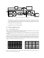
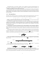
RTTY: an FSK decoder program for Linux.
Jesús Arias (EB1DIX)
June 15, 2001
Contents
1
rtty-2.0 Program Description.
1.1 What is RTTY . . . . . . . . . . .
1.1.1 The RTTY transmissions.
1.1.2 The program. . . . . . . .
1.1.3 System requirements. . . .
1.2 How the program works. . . . . .
1.2.1 General decoder structure.
1.2.2 The Digital filters. . . . .
1.2.3 Bit recovery. . . . . . . .
1.2.4 Character recovery. . . . .
.
.
.
.
.
.
.
.
.
2
2
2
2
2
3
3
4
5
5
2 User’s Manual.
2.1 Monitoring and Control Form. . . . . . . . . . . . . . . . . . . . . . . . . . . . . . . . . . .
2.2 Text-only mode. . . . . . . . . . . . . . . . . . . . . . . . . . . . . . . . . . . . . . . . . . .
2.3 The configuration file. . . . . . . . . . . . . . . . . . . . . . . . . . . . . . . . . . . . . . . .
6
6
6
6
.
.
.
.
.
.
.
.
.
.
.
.
.
.
.
.
.
.
.
.
.
.
.
.
.
.
.
.
.
.
.
.
.
.
.
.
.
.
.
.
.
.
.
.
.
.
.
.
.
.
.
.
.
.
1
.
.
.
.
.
.
.
.
.
.
.
.
.
.
.
.
.
.
.
.
.
.
.
.
.
.
.
.
.
.
.
.
.
.
.
.
.
.
.
.
.
.
.
.
.
.
.
.
.
.
.
.
.
.
.
.
.
.
.
.
.
.
.
.
.
.
.
.
.
.
.
.
.
.
.
.
.
.
.
.
.
.
.
.
.
.
.
.
.
.
.
.
.
.
.
.
.
.
.
.
.
.
.
.
.
.
.
.
.
.
.
.
.
.
.
.
.
.
.
.
.
.
.
.
.
.
.
.
.
.
.
.
.
.
.
.
.
.
.
.
.
.
.
.
.
.
.
.
.
.
.
.
.
.
.
.
.
.
.
.
.
.
.
.
.
.
.
.
.
.
.
.
.
.
.
.
.
.
.
.
.
.
.
.
.
.
.
.
.
.
.
.
.
.
.
.
.
.
.
.
.
.
.
.
.
.
.
.
.
.
.
.
.
.
.
.
.
.
.
.
.
.
.
.
.
Chapter 1
rtty-2.0 Program Description.
1.1 What is RTTY
1.1.1
The RTTY transmissions.
RTTY is a program that listen to your sound-card audio input and try to decode FSK modulated signals. These
signals can be found in HF bands and are commonly known as Radio-Tele-TYpe (RTTY).
In RTTY signals a given frequency is used to transmit a logic “1” and a different frequency is used for
the logic “0”. We call these frequencies MARK & SPACE frequencies respectively. The data format is those
found in asynchronous serial communications: Every character starts with a START bit with “0” logic value,
then follows the data bits, LSB first, and finally one or two STOP bits with a logic level “1” are added to the
character. Inter-character time is filled with a logic “1”. The character is often 5 bits long, and uses an old
encoding called BAUDOT, but sometimes a plain ASCII encoding is used. in this case the character is 7 or 8
bits long, and one optional parity bit can be added in order to check the received data integrity. The data rate is
slow. Typical values range from 42 to 300 baud.
1.1.2
The program.
The RTTY program, version 2.0 is not a complete “closed box” solution with all the features you think are
needed for an easy reception. Instead, the program has been designed with an academic purpose in mind, and
allows people to look what’s happening inside during reception.
This program is only suited for asynchronous communications. Other data formats, like AMTOR, PACTOR,
Weather data, etc. are not supported. In fact the program is able to recover those bit-streams, but i don’t know
very much about those data formats.
The program gives you a graphical interface that shows several signal traces in a window that resembles an
oscilloscope screen. This window helps to tune the incoming signals and also to identify some of its characteristics.
1.1.3
System requirements.
In order to run rtty-2.0 in your computer you will need at least:
• An Intel Pentium or compatible processor. The program requires very little CPU power. In a 166 MHz
Pentium it consumes only a 5% CPU time with a sampling rate of 44100 Hz. With lower sampling rates
(11025 Hz is the recommended minimum) the CPU use is negligible. This suggest that the program can
run in older computers, but this was not tested. Anyway, a hardware FPU is needed.
• A sound-card. Tested sound-cards are SoundBlaster-16 and SiS-7018 AC’97. The first one is an old card
and has an stable driver. The SiS-7018 is embedded in a laptop chipset. Its driver is still buggy.
• Linux Operating System. Of course.
2
FFT
Osciloscope
Audio
input
X
2
zero
crossing
+1
Lowpass filter
Bit
Recovery
DPLL
bandpass filters
BAUDOT/
ASCII
Terminal
Character
X
2
Recovery
-1
UART emulator
Demodulator
Figure 1.1: Block diagram of the rtty program.
• A sound-card driver. This driver can be compiled into the linux kernel or can be inserted as a module.
As previously stated, some drivers are buggy or lack some functionality. The SiS-7018 driver only
allows recording at 48 KHz sampling rate, and some “ioctl” calls are not implemented. As a result, the
oscilloscope window shows a poor animation.
• An X-window server for the graphical interface.
• An ANSI color terminal for the decoded output.
1.2
1.2.1
How the program works.
General decoder structure.
Figure 1.1 shows the block-diagram of the rtty program. It includes an FSK demodulation block, an UART
emulator block, a character terminal and some monitoring blocks.
The demodulator section takes audio samples as the input and generates a “0” or “1” logic level at the
output depending on the frequency of the input signal. This section is mainly based on digital filters, and works
as follows:
The input signal is filtered through a two bandpass filters. One filter is tuned to the MARK frequency while
the other is tuned to the SPACE frequency. As a result, two separated bands are obtained. Then, the “rms”
amplitude of each band is computed. This is achieved by squaring the band signals and then low-pass filtering
the result. The two “rms” amplitudes are then subtracted and the sign of the result is the logic output value. In
the actual implementation the subtraction and the low-pass filter are swapped, and only one low-pass filter is
needed. The response of such section is shown in figure 1.2.
0.5
0.6
(b)
(a)
0.4
0.4
0.3
0.2
0.1
Output (a.u.)
Output (a.u.)
0.2
0
-0.1
0
-0.2
-0.2
-0.3
-0.4
-0.4
-0.5
400
600
800
1000
1200
1400 1600 1800
Frequency (Hz)
2000
2200
2400
-0.6
2600
0
50
100
time (ms)
150
200
Figure 1.2: Demodulator response for a 1000Hz, 1850Hz, 75 baud configuration. (a) Frequency response, (b)
Time response to a pseudo-random bit stream.
3
The bandpass filters are second order “biquads”, with a Q adjusted to obtain the desired bandwidth. The
low-pass filter is implemented by two biquadratic sections, yielding an stopband attenuation of 80 dB/dec. The
bandwidth of all the filters is directly related to the data rate.
Following the demodulator is the UART emulator block. This section first tries to obtain a clock signal for
each bit in the DPLL block. Then, using this synchronization signal, the data bits are assembled according to
the data settings to obtain characters. These characters are checked against errors and then printed to stdout. If
the data length is 5 bits a BAUDOT encoding is assumed, and therefore the characters are translated to ASCII
before its printing.
1.2.2
The Digital filters.
The filters used in the RTTY program are of the IIR type. IIR means Infinite Impulse Response, which in turn,
means that the filter is implemented using some kind of feedback. The general IIR filter algorithm is:
yi = a0 xi + a1 xi−1 + ... + an xi−n + b1 yi−1 + ... + bn yi−m
(1.1)
Where xi is the current input sample and yi is the current output sample. As it can be seen, the current
output sample depends on the previous output samples, so here is the feedback.
The IIR filters are computer efficient, but they are very sensitive to coefficient accuracy and can become
unstable. To avoid instability, the order of the filter must be low. Higher order filters are implemented by
cascading lower order sections. In this program the filter section is order 2 and it is commonly called “biquad”.
The filter behavior is dictated by its own coefficients, and the calculation of these coefficients are the purpose
of the digital filter design.
The filter design starts with a continuous-time version of the biquad filter section, the resonant frequency,
ω0 , is “prewharped” to account for the further frequency response distortion. Then the Bilinear transform is
used to translate the continuous-time filter to a discrete-time version of the filter, where its transfer function is
written in terms of the Z transform. Finally the filter coefficients are derived from the discrete-time transfer
function.
In the following example a bandpass resonator is designed. The filter parameters are its resonant frequency
ω0 , and its quality factor Q. In order to account for the error introduced by the Bilinear
transform, the resonant
ω0
frequency is prewharped, so the used resonant frequency is: ω
b0 = 2fs tan 2fs , where fs is the sampling
frequency. The continuous-time transfer function, written in the Laplace transform terms, is:
H(s) =
s2
b
ω02
1 s
Qb
ω0
1 s
+Q
b
ω0
(1.2)
+1
Then, we use the Bilinear transformation to obtain an approximate discrete-time equivalent transfer func−1
tion. The Bilinear transform is merely the replacement of “s” by “2fs 1−z
1+z −1 ” in equation 1.2. The new transfer
function is then:
H(z) =
where α =
2α
Q (1
(4α2 +
2α
Q
− z −2 )
+ 1) + (2 − 8α2 )z −1 + (4α2 −
2α
Q
(1.3)
+ 1)z −2
fs
b
ω0
Then, the recurrence algorithm is derived taking into account that H(z) =
in the time domain by an n clock cycle delay. From equation 1.3 we obtain:
yi =
2α
Q
4α2 + 2α
Q
+1
(xi − xi−2 ) +
Y (z)
−n
X(z) , and that z
4α2 −
8α2 − 2
y
−
i−1
2α
4α2 + Q + 1
4α2 +
2α
Q
2α
Q
+1
+1
yi−2
is represented
(1.4)
And finally, by matching equation 1.4 with equation 1.1, the filter coefficients are easily obtained.
These bandpass resonators are used to split the signal into a mark & space bands in the very front-end of
the demodulator, but the demodulator also includes a low-pass filter, which is divided into two biquad sections
giving a total stopband attenuation of 80 dB/dec. Each section has the following transfer functions:
4
H(s) =
H(z) =
(4α2 +
2α
Q
1
s2
b
ω02
+
1 s
Qb
ω0
(1.5)
+1
1 + 2z −1 + z −2
+ 1) + (2 − 8α2 )z −1 + (4α2 −
2α
Q
(1.6)
+ 1)z −2
And the recurrence algorithm is:
yi =
1.2.3
1
4α2 +
2α
Q
4α2 −
8α2 − 2
(xi + 2xi−1 + xi−2 ) + 2 2α
yi−1 − 2
+1
4α + Q + 1
4α +
2α
Q
2α
Q
+1
+1
yi−2
(1.7)
Bit recovery.
The DPLL block accounts for the clock recovery from the demodulator output. But currently no clock signal
is generated. Instead the DPLL routine returns when the demodulator output shows a valid bit. A new call to
the DPLL routine does not return until a new bit has arrived.
The DPLL routine uses the “bit-phase” concept. The bit-phase is an static 16 bit integer variable that can
be incremented in a circular fashion. For each demodulator sample the bit-phase is incremented an amount that
is related to the data rate and the sampling frequency. When the bit-phase overflows the DPLL routine returns.
In order to get the bit-phase variable synchronized with the incoming bits some feedback is needed. In our
scheme the demodulator output must change only when the bit-phase is around its middle range value, that is
~32768, so, if a bit change is detected before this bit-phase value, the bit-phase is advanced 1/32 of its total
value. If the bit change takes place after the middle bit-phase value, the bit-phase is delayed 1/32 of its total
value. This feedback try to set the bit change around the middle bit-phase value, and thus, when the DPLL
routine returns, we are around the center of the bit time.
1.2.4
Character recovery.
The asynchronous serial data needs also a word synchronization. We wait for a falling edge in the demodulator
output that signals the beginning of a START bit. Then we wait for a half bit time and we check that the current
bit value is still “0”. If this check fails we just wait for another START bit.
When a valid START bit is detected we call the DPLL routine one time for each following bit. The data
bits, parity bit and STOP bits are recovered in this fashion. The recovered parity and STOP bits are checked
against errors and the character is marked as erroneous if this check fails. The character recovery routine waits
until all the STOP bits are read as “1” allowing for a more probably good START bit in the following character.
5
Chapter 2
User’s Manual.
2.1 Monitoring and Control Form.
Figure 2.1 shows the window that is opened after the program start. The window is divided in two parts. The
lower part includes several controls that allows us to select the desired data format and rate. The data rate can
be selected from a list of commonly used data rates, or it can be entered directly by typing it in the input filed.
The mark and space frequencies can be adjusted using four counter-buttons. The frequencies can be changed
in steps of 10 Hz or 100Hz. The bandwidth of the filters is made equal to the data rate.
The upper part of the form is a display that can plot several traces. This display can be just off if selected.
In figure 2.1 the trace selected shows the signal after the demodulation. The time scale is adjusted depending
on the data rate in order to show several bits.
The figure 2.2 shows the two other signals that can be plotted in the oscilloscope display. The first plot
shows the signal that is present at the input without any filtering. In this plot each horizontal pixel corresponds
to a new audio sample, and therefore the display shows 360 audio samples. In this example the input signal
was an FSK modulated square wave generated by a PIC16F84 microcontroller. The mark frequency was about
1850 Hz, the space frequency was 1000 Hz, and the data rate was 150 Hz.
The last plot of the figure 2.2 is the power spectrum of the previous signal. The vertical axis is logarithmic,
and shows 60 dB range. The plot also shows two rectangular bands that corresponds to the selected mark and
space frequencies. The space frequency is painted in red while the mark frequency is painted in green. The
width of these bands is the same as the filter bandwidth. As it can be seen in this plot, a properly tuned receiver
generates a signal spectrum that shows two peaks centered around the two filter frequencies. The width of the
peaks is also close to the bandwidth of the filters and proportional to the data rate. It must be noted that, due to
the square-wave nature of the incoming signal, a lot of small peaks are displayed in the spectrum display. This
is due to the high harmonic content of the square-wave signal that is folded back to low frequencies due to the
sampling in the PIC16F84.
2.2 Text-only mode.
The graphical interface can be disabled if the “-x” option is given in the command line arguments. Under these
circumstances the program setup can only be entered via configuration file (see section 2.3). This mode can be
useful for batch execution or when an X-window terminal is not available.
Note that even in text mode the program needs to link the “libX11.so.6” dynamic library. If you don’t want
to use the X-window environment nor library at all you must edit the “Makefile” file and recompile the source
code.
2.3 The configuration file.
When the program starts it try to read the data format, data rate and demodulator tuning from the “./rtty.cfg”
file. This file must be located in the current directory. This is a text file like the following one:
6
Figure 2.1: rtty form.
Figure 2.2: Oscilloscope display for input trace and spectrum respectively.
7
SPACEF=950
MARKF=1800
DR=150
NBIT=8
NSTOP=1
#-------- parity 0:none, 1:even, 2:odd ------PARITY=0
As it can be seen, each line contains a VARIABLE=VALUE statement. The equal character must be always
present and no spaces are allowed in the line. Comment lines start with the grid (#) character.
8