1
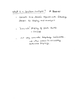
Spectrum Analyzer, Sampling Theorem and Amplitude Modulation 1 Objectives 1. Learn how to use a spectrum analyzer. 2. Study and understand the sampling theorem. 3. Study and understand how amplitude modulation (AM) works. 2 Theory 2.1 Spectrum Analyzer Like an oscilloscope, a spectrum analyzer produces a visible display on a screen. Unlike an oscilloscope, however, the spectrum analyzer has only one function-to produce a display of the frequency content of an input signal. (But it is possible to display the time waveform on the spectrum analyzer screen with the proper settings.) And also like an oscilloscope, the spectrum analyzer will always produce a picture on the screen; but if you do not know how to properly use the spectrum analyzer, that picture may be completely meaningless. CAUTION: The input of the spectrum analyzer cannot tolerate large signals; before you connect a signal to the input, be sure you know that the signal will not exceed the maximum allowable input rating of the spectrum analyzer. 2.1.1 Signal Acquisition in a Spectrum Analyzer Most spectrum analyzers are heterodyne1 spectrum analyzers (also called scanning spectrum analyzers). A heterodyne analyzer is essentially a radio receiver (a very sensitive and selective receiver). Given a voltage signal x(t), we need to somehow extract the frequency content out of it. As we know, the digital storage oscilloscope provides one solution as it can calculate the FFT of the signal from stored samples. Another solution would be to pass x(t) through a long series of very narrow bandpass filters, having adjacent passbands, and then plot the amplitudes of the filter outputs. That is, if filter 1 has passband f1 BW/2 < f < f1 + BW/2, and filter 2 has passband f2 - BW/2 < f < f2 + BW/2, where f1 + BW/2 = f2 BW/2, and so on, and if BW (the bandwidth) is small enough, then the filter outputs give us the frequency components X(f1), X(f 2), . . . and so on . This is, of course, not a practical solution. A better solution is suggested by a simple property of Fourier transforms: recall that if we multiply (in the time domain) a signal by a sinusoid, the spectrum of the signal is shifted in frequency by an amount equal to the frequency of the sinusoid. That is, 1 1 x(t ) cos(2πf 0t ) Fourier Transform → X ( f − f 0 ) + X ( f + f 0 ) 2 2 Now instead of a bank of narrow filters, we shall have one narrow filter centered at a fixed frequency, say fI, and we shall scan the signal spectrum across this filter by multiplying x(t) by a sinusoid of varying frequency f0 (See Figure 1). The filter is a narrow bandpass filter at a fixed center frequency, fI, (called the intermediate frequency); in a spectrum analyzer, its bandwidth is selected by the user. The oscillator frequency, f0, is adjustable, as indicated in Figure 1. In an ordinary AM or Figure 1: Frequency Mixing, or FM radio, when you tune the receiver you are selecting this Heterodyning frequency so that the desired signal will pass through the filter; in a spectrum analyzer, this frequency is automatically scanned (repeatedly) over a range, which must be selected so that the frequency component X(f) is shifted to fI and passed by the filter. For example, if we want to view the frequency content of x(t) from f1 to f2 , then we must select f0 to scan from f1 + fI to f2 + fI. 1 Heterodyne is derived from a Greek word meaning mixing different frequencies Of course, much more signal conditioning is going on inside the spectrum analyzer than is indicated in Figure 1; but the frequency mixing is the fundamental step. In particular, the signal first is passed through a lowpass filter whose bandwidth is chosen to eliminate image frequencies. Also, most scanning spectrum analyzers are multiple conversion analyzers - they have multiple intermediate frequency stages, at successively lower frequencies. The reason is that we have two conflicting goals to achieve; we would like to have the filter bandwidth as small as feasible, and we would like to be able to scan over large frequency ranges. It is hard to build sharp narrow filters at high frequencies, but it is also hard to build multipliers that will work over large frequency ranges. Therefore, we achieve narrow filters at low intermediate frequencies by shifting the frequency down in several steps. 2.1.2 Spectrum Analyzer Controls In this section we shall describe some of the basic controls on the spectrum analyzer that you will frequently use. More details on these, and descriptions of the more obscure controls, can be found in the user manual. Mainly, you will use the three large buttons labeled FREQUENCY, SPAN, and AMPLITUDE, the various MARKER buttons for making measurements, and the BW/Avg button for selecting the resolution bandwidth. In addition, you will use the control knob, the up and down buttons labeled with large arrows (above the control knob), and the numerical keypad for entering values that will control the display. When you use the spectrum analyzer, always pay attention to the in- formation about the instrument state given in the top, left, and bottom margins of the screen. FREQUENCY Control In normal operation the frequency control selects the range that the variable oscillator in Figure 1 sweeps through. Pressing the FREQUENCY button causes the frequency menu to appear on the screen. You can select the CENTER frequency (CF) and the START and STOP frequencies. You select the numerical values by turning the control knob, pressing the up/down arrows or by entering the value with the numerical keypad. SPAN Control Pressing the SPAN button brings up the frequency span menu. Here you select the frequency span displayed on the screen (as opposed to selecting start and stop frequencies), and you can select span zoom, zero span, and full span. AMPLITUDE / REF LEVEL Control Pressing this button displays the amplitude menu. Here you select the reference level, whether the amplitude units are power (dBm) or linear (mV), and the scale in dB/division (when using the logarithmic scale). Here is where the spectrum analyzer seems strange compared to an oscilloscope: you measure signal levels from the top of the screen, or down from the reference level. For example, on power-up, the reference level is 0 dBm, meaning that the top line on the screen is at 0 dBm and you measure the amplitudes of lines in the spectrum down from that level. For example, if the REF LEVEL is set to +10dBm, a signal peak that reaches the top of the display is +10dBm. The spectrum analyzer tends to provide more accurate readings when the input signal is placed in the upper two or so divisions of the display. Also, smaller REF LEVEL step sizes will provide more accurate measurements. Once again, you are cautioned to be careful about applying signals to the spectrum analyzer; it is easy to cause extensive and expensive damage. Resolution Bandwidth Control The resolution bandwidth is essentially the bandwidth of the fixed narrowband filter in Figure 1. (In reality, there are several stages of filtering.) Pressing the BW/Avg button displays the menu from which you can select the resolution bandwidth, the video bandwidth, and associated controls. Note that you cannot select a continuous range of RBW-there is only a finite selection available. The resolution bandwidth determines how close frequency components in the signal spectrum can be and still be displayed as distinct components on the screen. A large RBW may reveal only one signal, say at 900MHz. However, if the RBW is decreased, another signal at 899.5MHz may also be present (and thus will show up on the display). The AUTO button allows the spectrum analyzer to automatically select the RBW – manual selection is done with the UP/DOWN arrows – the AUTO button allows you to toggle between auto and manual RBW selection. Video Bandwidth (VBW) is basically a smoothing filter with a bandwidth equal to the RBW. VBW essentially reduces the noise displayed, making the power levels easier to see. VID FLTR button allows you to change the VBW. The sweep control is usually controlled by the spectrum analyzer (the rate at which different frequencies, f0 in Figure 1, are changed) but you can change this by using the arrows under the SWEEP heading. Markers Just as the oscilloscope has markers, the spectrum analyzer also has markers to help you make measurements. You select markers, difference markers, or no markers with the MARKER control buttons and their menus. 2.2 Sampling Theorem Sampling is the process of converting a signal (for example, a function of continuous time or space) into a numeric sequence (a function of discrete time or space). Shannon's version of the theorem states: If a function x(t) contains no frequencies higher than B cps, it is completely determined by giving its ordinates at a series of points spaced 1/(2B) seconds apart. A sufficient sample-rate is therefore 2B samples/second, or anything larger. Conversely, for a given sample rate fs the bandlimit for perfect reconstruction is B ≤ fs/2 . When the bandlimit is too high (or there is no bandlimit), the reconstruction exhibits imperfections known as aliasing. Modern statements of the theorem are sometimes careful to explicitly state that x(t) must contain no sinusoidal component at exactly frequency B, or that B must be strictly less than ½ the sample rate. The two thresholds, 2B and fs/2 are respectively called the Nyquist rate and Nyquist frequency. And respectively, they are attributes of x(t) and of the sampling equipment. The condition described by these inequalities is called the Nyquist criterion, or sometimes the Raabe condition. The theorem is also applicable to functions of other domains, such as space, in the case of a digitized image. The only change, in the case of other domains, is the units of measure applied to t, fs, and B. The symbol T = 1/fs is customarily used to represent the interval between samples and is called the sample period or sampling interval. And the samples of function x(t) are commonly denoted by x[n] = x(nT) (alternatively "xn" in older signal processing literature), for all integer values of n. The mathematically ideal way to interpolate the sequence involves the use of sinc functions. Each sample in the sequence is replaced by a sinc function, centered on the time axis at the original location of the sample, nT, with the amplitude of the sinc function scaled to the sample value, x[n]. Subsequently, the sinc functions are summed into a continuous function. A mathematically equivalent method is to convolve one sinc function with a series of Dirac delta pulses, weighted by the sample values. Neither method is numerically practical. Instead, some type of approximation of the sinc functions, finite in length, is used. The imperfections attributable to the approximation are known as interpolation error. Practical digital-to-analog converters produce neither scaled and delayed sinc functions, nor ideal Dirac pulses. Instead they produce a piecewise-constant sequence of scaled and delayed rectangular pulses (the zero-order hold), usually followed by an "anti-imaging filter" to clean up spurious high-frequency content. 2.3 Amplitude Modulation Amplitude modulation (AM) is a modulation technique used in electronic communication, most commonly for transmitting information via a radio carrier wave. AM works by varying the strength (amplitude) of the carrier in proportion to the waveform being sent. That waveform may, for instance, correspond to the sounds to be reproduced by a loudspeaker, or the light intensity of television pixels. This contrasts with frequency modulation, in which the frequency of the carrier signal is varied, and phase modulation, in which its phase is varied, by the modulating signal. In amplitude modulation, the amplitude or "strength" of the carrier oscillations is what is varied. For example, in AM radio communication, a continuous wave radio-frequency signal (a sinusoidal carrier wave) has its amplitude modulated by an audio waveform before transmission. The audio waveform modifies the amplitude of the carrier wave and determines the envelope of the waveform. In the frequency domain, amplitude modulation produces a signal with power concentrated at the carrier frequency and two adjacent sidebands. Each sideband is equal in bandwidth to that of the modulating signal, and is a mirror image of the other. Standard AM is thus sometimes called "double-sideband amplitude modulation" (DSB-AM) to distinguish it from more sophisticated modulation methods also based on AM. Single-SideBand modulation (SSB) or Single-SideBand Suppressed-Carrier (SSB-SC) is a refinement of amplitude modulation which uses transmitter power and bandwidth more efficiently. Amplitude modulation produces an output signal that has twice the bandwidth of the original baseband signal. Single-sideband modulation avoids this bandwidth doubling, and the power wasted on a carrier, at the cost of increased device complexity and more difficult tuning at the receiver. 3 Equipment 1. 2. 3. 4. 5. 6. Spectrum Analyzer Function Generator Oscilloscope AM experiment set DC power supply Modicom 1 board 4 Experiment Experiment 1 Spectrum Analyzer Experiment Procedure 1. Connect the function generator to the oscilloscope and apply the sine wave with frequency 200 kHz and magnitude 1 Vpp. 2. Connect the function generator to the spectrum analyzer and apply the sine wave with frequency 200 kHz and magnitude 0.5 Vpp and 2 Vpp, respectively. Record the results in both V and dBm units. 3. Repeat step 2 by changing the frequency to 100 kHz and 300 kHz, respectively. 4. Apply the square wave with magnitude 1 Vpp, duty cycle of 50% and frequency 100 kHz. Record the results in both V and dBm units. 5. Repeat step 4 by changing the frequency to 500 kHz. 6. Repeat step 4 by changing the duty cycle to 20%. Experiment 2 Sampling Theorem Experiment Procedure Turn off the power supply during circuit connection 1. Connect the power supply to the Modicom 1 board using the diagram shown in figure 2. Set the sampling control switch to “internal”. 2. Set the frequency of the sampled signal (p(t)) to 32 kHz by choosing 320 kHz (after divided-by10 circuit) and set the duty cycle to 1. 3. Apply a sine wave with Vp = 1 V and f = 12 kHz to the analog input of Modicom 1. Record the signals at sample output and sample/hold output in both time and frequency domains. 4. Change the duty cycle to 5 and repeat step 2-3. 5. Change the duty cycle back to 1 and change the frequency of the sine wave to f = 20 kHz, then repeat step 2-3. 6. Change the frequency of the sampled signal to 16 kHz (160 kHz on board) and repeat step 2-3. 7. Apply 1-kHz sine wave (test point 7) to the analog input. 8. Connect the sample output to second order and fourth order low pass filters (LPF). 9. Set the duty cycle to 1, change the sampling frequency to 2k, 4k, 8k, 16k and 32k, respectively, and record the output. 10. Change from sample output to sample/hold output and repeat step 8-10. Figure 2: DC power supply configuration Experiment 3 Amplitude Modulation Experiment Procedure Turn off the power supply during circuit connection 1. Connect the DC power supply to the AM transmitter board using the diagram shown in figure 1. 2. On the AM transmitter board, set AUDIO input Select to Int, MODE to DSB and Tx Output to Ant. 3. Adjust the signal from the audio oscillator to 1.5 kHz, 0.5 Vpp, then use the oscilloscope to record the signal at the test point 14. 4. Use the oscilloscope and the spectrum analyzer to record the signal from the 455 kHz crystal oscillator at the test point 16. 5. At the balanced modulator, adjust the balance knob to obtain the AM signal. Use the oscilloscope and the spectrum analyzer to record the signal. (HINT: Set the center frequency of the spectrum analyzer at 455 kHz) 6. Use the oscilloscope and the spectrum analyzer to record the signal at the test point 13. 7. Connect test point 17 to the test point 28, and set the switch detector to Diode. Use the oscilloscope to record the output. 8. At the balanced modulator, adjust the balance knob to obtain the DSB signal. Use the oscilloscope and the spectrum analyzer to record the signals at the test points 3 and 13. 9. Repeat steps 7. 5 Postlab Questions 1. What is an envelope detector? What are the advantage and the disadvantage of this detector? Also state its limitations. 2. How do spectra of sampled signal differ from those of sample/hold signal? Also explain why.