Download Timing Margin Recovery With Flexible Flip

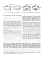
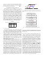
Timing Margin Recovery With Flexible Flip-Flop
Timing Model
D
tsetup
clk
clk
Q
Flop
D
Q
+
thold
tc2q
Andrew B. Kahng† and Hyein Lee†
†
+
ECE and CSE Departments, University of California at San Diego
[email protected], [email protected]
I. I NTRODUCTION AND M OTIVATION
Timing signoff with static timing analysis (STA) is critical to ensure functionality and required performance of a
design, and is a cornerstone of handoff from design house
to foundry. Designers spend enormous effort to remove fewpicosecond timing violations, using ECO (engineering change
order) knobs such as threshold voltage (Vt) swap, gate width or
channel length sizing, and buffering/cloning transforms. This
increases design turnaround time, decreases design quality
(e.g., due to more power consumption from inserted buffers)
and results in larger die sizes. At the post-routing stage,
ECOs based on extracted parasitics (SPEF) become harder
and potentially disrupt convergence; this is because the entire
design is almost fixed, and even a small sizing change can
require placement legalization and search-repair in detailed
routing. As a result, to avoid as many late-stage ECOs as
possible, designers seek to recover every possible picosecond
of unneeded timing margin. An example of this is seen in the
use of path-based analysis (PBA) options in final signoff STA,
since this is less pessimistic (albeit more time-consuming) than
graph-based analysis (GBA).
To verify timing correctness of a flip-flop based sequential
circuit, STA checks for two types of timing constraints – setup
D
tsetup
clk
clk
Q
Flop
Fig. 1.
thold
D
Q
tc2q
Setup time, hold time and c2q delay of a flip-flop.
160
160
44
150
150
42
140
140
130
130
120
120
110
110
100
100
90
90
80
80
0
50
hold time [ps]
100
hold time [ps]
c2q delay [ps]
Abstract—In timing signoff for leading-edge SOCs, even
few-picosecond timing violations will not only increase design
turnaround time, but also degrade design quality (e.g., through
power increase from insertion of extra buffers). Conventional
flip-flop timing models have fixed values of setup/hold times
and clock-to-q (c2q) delay, with some advanced “setup-hold
pessimism reduction” (SHPR) methodologies exploiting multiple
setup-hold pairs in the timing model. In this work, we propose to
use multiple timing models to give more flexibility at timing path
boundaries, thus recovering significant “free” margins and reducing the number of timing violations that require unnecessary
fixes. We exploit a flexible flip-flop timing model that captures the
three-way tradeoff among setup time, hold time and c2q delay, so
as to reduce pessimism in timing analysis of setup- or hold-critical
paths. A sequential linear programming optimization for multiple
corners is used to selectively analyze setup- or hold-critical paths
with less pessimism. Further improvements are possible based
on partitioning of timing paths according to different modes.
We demonstrate that our method can improve worst setup/hold
slack metrics over conventional signoff methods, using a set of
open-source designs implemented in a 65nm foundry library. We
show that opportunity for timing pessimism reduction with our
approach remains significant in a 28nm FDSOI foundry library
as well.
40
38
36
34
32
30
0
50
100
setup time [ps]
0
20
40
60
80
setup time [ps]
Fig. 2. From left to right: (i) c2q delay versus setup time, (ii) c2q delay
versus hold time, and (iii) setup time versus hold time. A DFQDX flip-flop
in 65nm foundry technology is used for the SPICE simulation.
UCSD VLSI CAD Laboratory
time and hold time. As shown in Figure 1, STA must guarantee
that the logic value has been stable at the data input by setup
time (tsetup ) before it is captured by the clock edge. On the
other hand, the logic value must be maintained for hold time
(thold ) after the capturing clock edge to ensure that the flipflop will store the correct value. The two constraints form
a timing window during which the flip-flop can capture the
data correctly [9]. STA checks maximum- and minimum-delay
combinational paths to ensure that the logic value will be ready
and stable in this timing window. After correct capture of the
logic value, there is a clock-to-q (c2q) delay (tc2q ) during
which the captured value propagates to the flip-flop output,
as shown in Figure 1.
In the conventional timing library characterization flow,
setup and hold time are characterized independently, after applying a pushout criterion whereby the c2q delay is degraded
by 10%. During the characterization of setup time, hold time
is assumed to be infinite, and vice versa. Also, c2q delay is
characterized with a constant data input, which corresponds
to both setup time and hold time being infinite. There are
substantial impacts of hold time, setup time and c2q delay
on each other, which the conventional characterization flow
cannot capture. For example, Figure 2 shows (i) c2q delay
19
FF3
FF2
480ps
A Counter Example to [ChenLS12]
{10,20}
{10,20}
(b)
Available FF timing model:
{hold time, c2q} = {30,0}, {20,10}
20ps
FF1
20ps
FF1
FF2
①
Not feasible
with either {30,0} or {20,10}
(a)
path1={10,20}
path2={10,20}
①
give c2q delay +10ps
= min delay = 20ps
10ps
③
FF3
give c2q delay +10ps
= min delay = 30ps
20ps
{30, 0}
Available solution:
{setup time, c2q}
= {20,10}, {10,20}
FF2
②
{20,10}
(b)
path1,2={10,20}
FF1
FF1
480ps
480ps
20ps
10ps
FF3
{20,10}
470ps
470ps
FF3
path1={20,10}
path2={10,20}
460ps
480ps
470ps
470ps
clock period=510ps
460ps
clock period=500ps
FF3
FF2
path1={10,20}
path2={20,10}
path1,2={10,20}
460ps
480ps
460ps
FF2
path1,2={10,20}
(b)
(a)
UCSD VLSI CAD Laboratory
Fig. 3.
(a) Suboptimality of iterative search. (b) Optimal solution.
versus setup time, (ii) c2q delay versus hold time, and (iii)
setup time versus hold time, according to SPICE simulation
with a DFQDX flip-flop from a 65nm foundry library. The c2q
Laboratory
delay rapidly increases UCSD
whenVLSI
theCAD
setup
or hold time is smaller.
In the conventional timing analysis, this region is disregarded
by the fixed 10% pushout criterion.
Works such as [3] have pointed out that the interdependency
among setup time, hold time and c2q delay should be considered to achieve accurate flip-flop timing characterization.
Focusing on setup-hold time interdependency, several characterization methods [3] [7] and applications in timing analysis
[3] [4] [5] [1], including statistical STA (SSTA) [2], have been
proposed. Going beyond the setup-hold tradeoff, Chen et al.
[1] propose an iterative timing analysis that exploits the additional tradeoff with c2q delay. They achieve 3-4% reduction
in clock period through a new modeling methodology for flipflop timing.
Two Motivating Observations. Our research seeks “free”
design margin reductions through improved path-based static
timing analysis with flexible flip-flop timing model. As detailed below, our work is closest to that of [1], but we propose
a better exploitation of the three-way setup-hold-c2q tradeoff.
We further propose to improve timing margins by separately
considering the multiple corners and modes that are intrinsic
to timing signoff of any real IC design. Two motivating
observations lead us in these directions.
Observation 1: suboptimality of iterative search over setuphold pairs. Iterative search for the best setup-hold pair for
each flip-flop instance, which is proposed by Chen et al. [1], is
straightforward and can be easily adopted into timing signoff.
However, we find that this approach may not produce an
optimal solution for the overall design, depending on initial
conditions and the order in which iterations are made. For
example, suboptimality can occur when an initial condition is
too pessimistic so that the optimization cannot be performed
further. Figure 3 gives a counterexample for the method of
[1] showing that iterative search can result in a suboptimal
solution for hold time constraints. In the example, we assume
that two pairs of {hold time, c2q} values are possible: {30, 0},
{20, 10}. If the iterative search algorithm first tries to assign
a (hold, c2q) to FF2 , as in Figure 3(a), a feasible solution
cannot be found since the minimum delay (10ps) is too short
for either of the available {hold time, c2q} pairs. (Given the
Fig. 4. (a) Mode-specific PBA signoff (Example 1). (b) Non-mode-specific
PBA signoff (Example 2).
two options for hold time, 30ps and 20ps, if the minimum
delay is 10ps, a hold time violation occurs with either option.)
However, if the algorithm were to try FF1 first, the {20,10}
timing model
option could be assigned, with this giving a c2q
3
delay of 10ps; this increases the minimum delay between FF1
and FF2 , thus enabling FF2 to have a feasible timing model
option as well. In this way, we can assign feasible solutions
for all flip-flops as shown in Figure 3(b).
Observation 2: disjointly analyzable paths in timing signoff.
When flexibility in the flip-flop timing model is enabled,
a key intuition is that disjointly analyzable timing paths –
specifically, in path-based analysis (PBA) with multiple modes
– enable more exploitation of the flexibility. We illustrate this
concept in Figure 4. In the figure, suppose that the solid-line
(white icons) and dashed-line (gray icons) paths (path1 and
path2, respectively) are independent of each other with respect
to timing analysis. We assume that only the paths indicated by
same kinds of line can be sequentially adjacent, so that there
are different timing slacks depending on the dashed/solid line
(i.e., mode). The timing slack of a timing path determines
setup margin, which is the required setup time of the flip-flop
at the endpoint of the timing path, as well as the corresponding
c2q delay. The timing slack of the following timing path
is used to check whether the c2q delay determined by the
preceding timing path is applicable (i.e., feasible). Then, the
possible room for time borrowing from the following path is
determined by its timing slack. Two realistic design scenarios
show the relevance of these assumptions. (1) First, either the
solid-line paths or the dashed-line paths can be disabled by
control signals, depending on modes. For example, designs
with scan-based test logic contain scan chain paths which are
independent from logic paths: logic paths will be disabled
during scan mode, and scan chain paths will be disabled
during function mode. (2) Second, there can be input vector
dependencies. Suppose that the solid-line paths are enabled by
input 1 and always produce input 1. Similarly, suppose that the
dashed-line paths are enabled by input 0 and always produce
input 0. In this situation, based on the input vectors, only sametype paths can be simultaneously enabled. Non-mode-specific
PBA cannot differentiate between solid-line and dashed-line
paths in either of these design scenarios, and this can cause
pessimistic results in timing signoff. Section V below presents
results with designs that have inserted test logic, exemplifying
(1).
4
...
...
hold
Figure 4(a) illustrates how choosing
different setup-c2q
fixed timing model
hold
pairs according to the disjoint analyzability of paths can
improve the achievable minimum clock period. We assume
setup-hold
that two available {setup time, c2q} pairs are {20,10}flexible
andmodel
{10,20}. A clock period of 500ps is achieved when each FF c2q1
c2q1
setup-hold-c2q
can be assigned different pairs for each of path1flexible
and model
path2,
setup-hold-c2q
flexible model
so that each path independently exploits the flexible timing c2q
fixed timing
n
model
c2qn
model. However, with a rigid timing model, as shown in
setup-hold flexible model
Figure 4(b), when both solid-line and dashed-line paths are setup
setup
constrained to have one common setup-c2q pair choice at each Fig. 5. The space of setup, hold and c2q for each type of flip-flop timing
flip-flop, the clock period cannot be reduced from 510ps.1
model.
Scope and Organization of Paper. Given the above mo- and the contour lines represent available setup-hold pairs that
tivating observations, in this work we make the following give a certain c2q delay (c2qn ). With the fixed setup-hold time
contributions.
model, which is used in conventional STA, only one triplet of
• We develop a sequential linear programming (LP) based
(setup, hold, c2q) is available, as shown as the black dot. With
optimization to reduce pessimism in timing signoff at the flexible setup-hold time model, proposed in [3], multiple
both setup-critical (max) and hold-critical (min) corners. setup-hold time pairs are available to use (as indicated by
• We demonstrate that further margin optimization can be
the blue line), at a particular c2q delay. Beyond this, having
achieved by using path partitioning according to mode in flexible c2q delay allows to broaden the solution space for
mode-specific path-based analysis.
the (setup, hold c2q) triplet to multiple c2qn contours. This
UCSD
VLSI CAD Laboratory
18
• Experimentally, using a set of open-source designs
impleflexibility enables a better global optimization across all timing
mented in a 65nm foundry technology, we demonstrate paths.
that our method improves worst slack (WS) by an average
of 48ps and by up to 130ps, compared to conventional Timing corners and modes. In conventional static timing
analysis-based signoff, circuit timing is analyzed at various
fixed timing model-based analysis.
process, voltage and temperature (PVT) corners. Among the
• We further show that our analysis based on flexible flipflop timing model improves WS metrics when compared various signoff corners corresponding to different PVT comto the earlier work of [4] as well as to a pessimism binations, setup time is checked at one or more max corners,
reduction analysis option (based on setup-hold flexibility) i.e., the corner(s) where timing delays take on their maximum
in the 2013 version of a commercial timing analysis tool. value(s). On the other hand, hold time is checked at one or
The rest of this paper is organized as follows. In Section more min corners, i.e., the corner(s) where timing delays take
II, we summarize required concepts of flip-flop taxonomy and on their minimum value(s). At any given corner, there can
timing signoff analysis. In Section III, we briefly review re- be multiple modes for timing analysis. That is, a design may
lated literature. Section IV describes our problem formulation have different operating modes (turbo functional mode, scan
and proposed methodology, Section V presents our experi- test mode, etc.), as well as different functionalities according
mental setup, overall flow including flip-flop characterization to its input signals. Timing analysis must be performed with
and proposed timing signoff, and experimental results. We all possible corners and modes to ensure design functionality
conclude the paper and note ongoing research direction in at all conditions. However, due to limited resources, product
engineering and design teams may choose some subset of
Section VI.
potential corners and modes, perhaps in combination with
II. BACKGROUND T ERMINOLOGY
some pessimism, such that all conditions are covered. In
Before proceeding further, we briefly set out relevant termi- our experimental studies reported below, we use two signoff
nology regarding flip-flop timing models, and the concept of corners, i.e., min and max corner, and two modes, i.e., function
and test mode.
timing mode and corner.
Taxonomy of flip-flop timing models. In this paper, we
discuss three kinds of flip-flop timing models:
• Fixed setup-hold time;
• Flexible setup-hold time; and
• Flexible setup-hold time and c2q
Figure 5 illustrates all three types of flip-flop timing model;
in the figure, the x-axis is setup time, the y-axis is hold time,
1 In Figure 4(b), if there are two timing model options for each flip-flop,
eight distinct assignments of timing model to flip-flop are possible. The point
here is that with any of the eight assignments, the clock period is 510ps
because the assignments are not made independently for the path1 (solid line)
and path2 (dashed line) analyses.
III. R ELATED W ORKS
We now review related literature on the characterization
and utilization flexible flip-flop timing models discussed in the
preceding section. Most of these previous works propose not
only characterization, but also application, of flexible flip-flop
timing models.
Figure 6 gives a taxonomy of previous works, and their
relation to our present work. We divide related works into
four categories according to two axes: (1) two types of flipflop timing models – flexible setup-hold timing model and
flexible setup-hold-c2q timing model – which are discussed in
analysis pessimism. For example, Synopsys PrimeTime [17]
supports a Setup Hold Pessimism Reduction (SHPR) analysis
option. The tool optimizes setup (resp. hold) slack at the
expense of hold (resp. setup) slack, by using multiple pairs
setup[1]
of setup and hold time that are described in the Libertyhold[our work]
format [12] timing library. Safer et al. [2] apply codepenc2q
dent setup/hold times to statistical timing analysis. In [2],
setup[1] [2] [3] [4]
[7] [8] [10]
hold
[5] [6] [our work]
probability mass functions of setup/hold times for each flipflop instance, along with setup/hold margins, are computed
Characterization
Timing analysis
to obtain the probability of failure for each timing endpoint
Fig. 6. Taxonomy of previous works, and the scope of this work.
(typically, flip-flop inputs and primary outputs of the circuit).
(ii) With setup-hold-c2q timing model. Chen et al. [1] suggest
Section II, and (2) two applications, i.e., characterization and
iterative timing analysis based on nonlinear and interdependent
timing analysis including both STA and statistical STA. The
flip-flop modeling. They model c2q delay as an analytical
flexible setup-hold-c2q timing model can be also viewed as
function of setup/hold times, load capacitance and clock skew,
subsuming the setup-hold timing model, since the latter is a
and utilize this in their iterative STA method. The iterative
restriction (special case) of the former.
STA starts with an initial c2q delay for each flip-flop and
Flexible flip-flop timing model characterization. Works in recomputes this c2q delay using the analytical function, i.e.,
this category propose methods for characterization of setup- based on the flip-flop’s setup and hold margins, and load
hold interdependency.
capacitance. The iterative STA method tells whether or not the
(i) With setup-hold timing model. Rao and Howick [10] give a circuit can meet a given clock period; then, a minimum feasiUCSD
CAD
Laboratory
method to obtain a pair of setup and
holdVLSI
times,
using
a two- ble clock period is obtained with binary20search. We categorize
step characterization method and considering setup-hold inter- our work with that of [1]: we also pursue timing analysis with
dependency, to overcome optimism in conventional setup-hold a flexible setup-hold-c2q timing model. However, we suggest
characterization. They resolve the optimism that stems from more effective global optimization of timing slack using a
assuming infinite counterpart skew, i.e., setup (resp. hold) skew sequential LP method. Also, going beyond the four categories
for hold (resp. setup) time characterization. However, they do of our taxonomy, we suggest new timing analysis methods,
not exploit the interdependency to reduce possible pessimism namely, mode-/corner-specific timing analysis (shown as an
in STA. Srivastava and Roychowdhury [7] [8] propose a rapid oval in Figure 6), that can exploit the two types of flexible
and accurate setup-hold time characterization methodology flip-flop timing models2 .
by using Euler-Newton Curve Tracing. The proposed method
achieves 26× speedup over a surface generation/intersection
IV. P ROBLEM F ORMULATION AND M ETHODOLOGY
method. However, timing optimization/analysis methods are
not discussed in this category of previous works. Moreover,
We now describe the problem formulation for a sequential
no work explicitly addresses the characterization of the threeLP-based
optimization. Table I presents the notations that are
way tradeoff, i.e. setup-hold-c2q timing model.
used in our problem formulation. Our objective is to find the
New timing analysis with flexible flip-flop timing model. best triplet of setup, hold and c2q for each flip-flop to minimize
Works in this category propose applications of interdependent setup/hold timing violations.
setup-hold or setup-hold-c2q timing models.
TABLE I
(i) With setup-hold timing model. Salman et al. [3] propose a
N OTATIONS
method to reduce pessimism in timing analysis by exploiting
Notation
Meaning
setup-hold interdependency. In [3], required setup and hold
P
clock period
times (i.e. setup and hold slacks) for each flip-flop instance is
Tsu (i)
setup time of flip-flop i
Th (i)
hold time of flip-flop i
calculated, and the best match among pre-characterized setupcsu (i)
specified setup time of flip-flop i
hold pairs is selected. With the proposed method, the number
ch (i)
specified hold time of flip-flop i
of setup and hold violations can be reduced. However, the
Tcq (i)
c2q delay of flip-flop i
Usu
maximum setup time
proposed algorithm simply matches the best setup-hold pair
Uh
maximum hold time
for each flip-flop with respect to direct flop-to-flop timing
Lsu
minimum setup time
paths. It does not consider the interaction among timing paths,
Lh
minimum hold time
Ssu
worst (i.e., minimum) setup slack
i.e., there is no global optimization. Salman and Friedman
Sh
worst (i.e., minimum) hold slack
[6] propose an improved STA that considers variation by
fc2q (s, h)
analytic model of c2q delay w.r.t. setup time s, hold time h
utilizing interdependent setup/hold time. They recover lost
dmax (i, j)
maximum path delay between flip-flop i and j
dmin (i, j)
minimum path delay between flip-flop i and j
signoff margin arising on data paths due to power noise and
threshold voltage variation, by exploiting the tradeoff between
2 We believe that the new methods do not fall into any of the four categories,
setup and hold time. Commercial timing analysis tools can as the mode-/corner-specific timing analysis is inherently different from the
also comprehend interdependent setup-hold times to reduce conventional timing anaysis.
mode-/cornerspecific STA
[our work]
Sequential LP-based optimization. We divide the original
problem into two optimization problems, i.e., setup-c2q optimization and hold-c2q optimization, to enable LP formulation.
Since it is hard to find an accurate linear model for the setuphold-c2q surface, each optimization exploits one-dimensional
tradeoff, i.e., setup-c2q and hold-c2q, with a reduced complexity.
Problem : setup-c2q optimization (SC2QOpt)
(1)
Maximize : Ssu
Subject to : fc2q (Tsu (i), ch (i)) + dmax (i, j) + Tsu ( j) + Ssu ≤ P
(∀pair(i, j))
Lsu ≤ Tsu (i) ≤ Usu
Problem : hold-c2q optimization (HC2QOpt)
(2)
Maximize : Ssu + Sh
Subject to : fc2q (csu (i), Th (i)) + dmax (i, j) + csu ( j) + Ssu ≤ P
(∀pair(i, j))
dmin (i, j) + Sh > Th (i)
Lh ≤ Th (i) ≤ Uh
The setup-c2q optimization is described in Problem (1). The
objective is to maximize Ssu so that the setup time violation
can be minimized. In this problem, we assume that the hold
time for each flip-flop ({ch (i)}) is given and we do not try
to minimize hold time violations, but to keep the current
hold slack. Hold time violations are reduced in the holdc2q optimization (Problem (2)). The objective is maximizing
the sum of the worst setup and hold slack values. In this
stage, with a given fixed setup ({csu (i)}), optimized holdc2q pairs are determined to minimize the sum of setup and
hold time violations by utilizing the tradeoff between c2q and
hold time. The two optimizations are performed sequentially
in Algorithm 1.
Timing signoff across corners. At the max corner, setup
time is more critical while hold time violation rarely occurs,
and vice versa at the min corner. Thus, depending on signoff corners, we selectively analyze setup- or hold- critical
paths, i.e., focusing on reduction of setup time pessimism
at the max corner, and focusing on reduction of hold time
pessimism at the min corner. Algorithm 1 describes the timing
signoff flow at the max corner (STA FTmax ) and the min
corner (STA FTmin ). The two optimizations SC2QOpt(C,V )
and HC2QOpt(C,V ) respectively solve Problem (1) and Problem (2): each returns a solution (sol), which contains setup
(sol.setup), hold (sol.hold) and c2q delay (sol.c2q) values for
each flip-flop, with given timing constraint sets C and fixed
timing values V (can be hold or setup). In STA FTmax , the
maximum path for each flip-flop pair is collected (Line 3)
and fed into SC2QOpt with the maximum possible hold time
values, i.e., the hold slack for each flip-flop (Line 5). Then,
with respect to hold time constraints, SC2QOpt obtains the
best setup-c2q pairs. Then, we annotate setup, hold and c2q
according to the result of SC2QOpt. At the second phase,
we collect all paths that have hold time violations and apply
Algorithm 1 Timing signoff flow at max/min corner.
Procedure STA FTmax (G)
Dmax ← 0/
for all flip-flop pair (i, j) do
Dmax ← Dmax ∪ dmax (i, j);
end for
{sol} = SC2QOpt(Dmax , {ch });
for all flip-flop i s.t. ∃sol(i) do
Annotate sol(i).setup, sol(i).c2q;
end for
Dmin ← 0/
for all flip-flop pair (i, j) do
if hold time violation occurs with dmin (i, j) then
Dmin ← Dmin ∪ dmin (i, j);
end if
end for
{sol} = HC2QOpt(Dmin , {csu });
for all flip-flop i s.t. ∃sol(i) do
Annotate sol(i).hold, sol(i).c2q;
end for
Procedure STA FTmin (G)
1. Dmin ← 0/
2. for all flip-flop pair (i, j) do
3.
Dmin ← Dmin ∪ dmin (i, j);
4. end for
5. {sol} = HC2QOpt(Dmin , {csu });
6. for all flip-flop i s.t. ∃sol(i) do
7.
Annotate sol(i).hold, sol(i).c2q;
8. end for
9. Dmax ← 0/
10. for all flip-flop pair (i, j) do
11.
if setup time violation occurs with dmax (i, j) then
12.
Dmax ← Dmax ∪ dmax (i, j);
13.
end if
14. end for
15. {sol} = SC2QOpt(Dmax , {ch });
16. for all flip-flop i s.t. ∃sol(i) do
17.
Annotate sol(i).setup, sol(i).c2q;
18. end for
1.
2.
3.
4.
5.
6.
7.
8.
9.
10.
11.
12.
13.
14.
15.
16.
17.
18.
HC2QOpt for those paths. Note that we use the setup (csu )
values that are obtained from the previous optimization. The
solutions from HC2QOpt are annotated to each flip-flop for
the final timing signoff.
In STA FTmin , we first collect the minimum path for each
flip-flop pair. Then, we apply HC2QOpt to minimize hold time
violations while maintaining setup delay. Last, SC2QOpt is
performed to reduce possible setup time violations by trading
off between c2q and setup slack.
Timing signoff across modes. As discussed in the motivating
Observation 2 in Section I, exploiting flexible flip-flop timing
model can be beneficial for timing analysis with multiple
modes. For example, in scan (shift) mode, the likelihood
that hold time violations occur is significantly higher than
for setup, since the frequency is reduced in this mode and
hence there is no setup-criticality. This is because the scan
path between flip-flops has a smaller number of logic stages
compared to normal functional paths. If we use a fixed timing
model for both modes, we would end up with extra buffer
insertion in scan mode to fix hold time violations. To obtain
clock
proper sets of setup-hold values and independently minimize
hold time violations for each mode, we perform STA FTmin
in scan and function mode separately.
setup time
data
input
V. E XPERIMENTAL S ETUP AND R ESULTS
We have applied our proposed method on a set of opensource designs. All designs are synthesized from RTL, and
scan logic is inserted, using Synopsys Design/DFT Compiler
H-2013.03-SP3 [15]. For P&R, we use Cadence Encounter
Digital Implementation System XL 10.1 [11]. Implementations
in all experiments are with a 65nm foundry technology and
library. Synopsys PrimeTime H-2013.06-SP2 [17] and CPLEX
12.5.1 [14] are respectively used as the timing tool and the
LP solver in our experiments. Table II summarizes relevant
parameters of testcases including the number of instances and
registers. The output netlist and extracted SPEF file from
P&R are used for the timing analysis in our experiments. The
proposed timing analysis flow is implemented using Tcl/Tk
8.4 [18] scripting and the Synopsys PrimeTime interface.
Fig. 7. Input and output waveform for setup-hold-c2q characterization. To
consider interdependency of setup-hold, a pulse input is used instead of ramp
input.
Netlist (and SPEF, if routed)
data
setup time = ∞
Extract path timing information
min. hold time
LP formulation
with flexible flip-flop timing model
Solve Sequential LP
(STA_FTmax , STA_FTmin)
Solution
UCSD VLSI CAD Laboratory
Annotate new timing model
for each flip-flop
testcase #instances #registers
tv80s
4843
359
aes
15622
530
conmax
24856
818
dma
25529
1051
jpeg
70074
4936
Timing signoff with annotated timing
Fig. 8.
The interdependency among setup, hold time and c2q delay
of a flip-flop is characterized according to the method in
[10] by using Synopsys HSPICE [16] with the 65nm foundry
library. Through an extensive and exhaustive search, we obtain
a large set of triplets of setup, hold time and c2q for each
combination of data, clock slew and load capacitance. Figure 7
shows the input and output waveform for setup-hold-c2q
characterization. In contrast to the conventional use of a ramp
input assuming infinite setup (resp. hold) time for hold (resp.
setup) characterization, we use a pulse input in light of the
interdependency of setup and hold.
Linear approximation. To obtain an analytic model of c2q
( fc2q (s, h)) for the LP formulation in Section IV, we approximate the contours of setup-c2q, hold-c2q and setuphold as linear lines. Through an extensive SPICE simulation,
these contours are obtained at every 5ps of timing points,
where setup and hold time are characterized over the range of
5ps ∼ 200ps. We recognize that that the linear approximation
of the non-linear curves has inherent inaccuracy that can result
in optimism or pessimism in the timing analysis; improving
this is a direction of ongoing work.
Linear interpolation for load and input slew. The cost of
characterization of the flip-flop timing is high since multiple
pass-fail-based trials are required to determine setup and hold
time. Moreover, as the characterization of the setup-holdc2q tradeoff surface is required at each combination of load,
data and clock slew, the characterization cost can increase
dramatically. Due to practical limits on characterization effort,
hold time
data slew clock slew
TABLE II
T ESTCASES : THE NUMBER OF INSTANCES AND REGISTERS .
A. Characterization
q output
c2q
New timing signoff flow with flexible flip-flop timing model.
UCSD VLSI CAD Laboratory
we use linear interpolation to obtain the setup-c2q or hold-c2q
tradeoff curve, for any non-characterized load, clock slew and
data slew points.
B. New timing signoff flow with flexible flip-flop timing model.
Figure 8 presents the proposed timing signoff flow with
the flexible flip-flop timing model. Based on the input netlist
and extracted interconnect parasitics, we run timing analysis
to extract the maximum and minimum delays of all flop-toflop timing paths. Solving the LP of Section IV determines
the setup-hold-c2q solution for each flip-flop. These optimized
timing models are annotated to each flip-flop to obtain a more
accurate timing signoff with reduced pessimism.
Design of experiments. We have studied the following scenarios to evaluate our methodology. STA FTmax and STA FTmin
in Algorithm 1 are used for max and min corner analysis on
the designs that have timing violations at a particular corner.
Experiments 1 and 2 emulate general timing signoff cases.
At the max corner, as the data path delay becomes larger,
setup time violations occur whereas hold time violations rarely
happen. In the same manner, at the min corner, hold time
violations usually occur but there are few setup time violations.
In Experiments 3 and 4, we also examine extreme cases, where
both setup and hold violations occur at either max or min
corner. We generate -30ps∼-140ps initial setup/hold violations
for the experiments. Table III shows the initial setup/hold slack
values, in nanoseconds, for all the experiments.
0.050
tv80s
aes
conmax
dma
jpeg
0.160
conventional
[4]
cTool
0.000
0.080
0.060
[4]
cTool
proposed
1.200
conventional
[4]
cTool
proposed
setup slack
0.000
tv80s
aes
tv80s
aes
conmax
hold slack
conmax
dma
jpeg
dma
0.020
jpeg
-0.060
0.400
-0.080
-0.080
0.200
-0.100
-0.100
-0.120
-0.120
setup slack
dma
jpeg
-0.140
conventional
(b)
[4]
cTool
proposed
Experiment 5 studies the mode-specific timing analysis as
an example of disjointly analyzable paths in timing signoff,
which is discussed in Observation 2 in Section I. As timing
path delay varies across modes, a flexible timing model is
required to obtain an optimized timing analysis. The discrepancy of timing path delay depending on modes will be
maximized when test and function mode are considered, since
scan paths usually suffer from hold time violations due to their
relatively small number of stages. Thus, in our experiment, we
synthesize test logic to enable scan mode. Experiment 5 uses
the same scenario as Experiment 3 (i.e., both setup and hold
time violations at max corner). However, according to modes,
setup or hold time violations can be removed, as some of
paths become false paths in a particular mode, if they are not
enabled in that mode. Thus, with Experiment 5 we are able to
demonstrate that further reductions of timing pessimism are
possible using mode-specific signoff analysis.
•
•
•
•
•
Experiment 1 (exp1): setup time violations at max corner
Experiment 2 (exp2): hold time violations at min corner
Experiment 3 (exp3): setup and hold time violations at
max corner
Experiment 4 (exp4): setup and hold time violations at
min corner
Experiment 5 (exp5): setup time violations at function
mode, hold time violations at test mode, at the same
corner
TABLE III
I NITIAL SETUP / HOLD SLACK VALUES (ns) FOR E XPERIMENTS 1–5.
exp1
setup hold
tv80s -0.100 0.109
aes
-0.141 0.084
conmax -0.100 0.105
dma
-0.115 0.085
jpeg
-0.101 0.082
testcase
exp2
setup hold
1.000 -0.080
0.713 -0.100
1.000 -0.080
0.708 -0.080
1.087 -0.119
exp3/5
setup hold
-0.100 -0.080
-0.141 -0.100
-0.100 -0.081
-0.115 -0.080
-0.101 -0.103
tv80s
-0.140
exp4
setup hold
-0.100 -0.080
-0.100 -0.100
-0.100 -0.080
-0.100 -0.080
0.007 -0.099
Experiment 1 – 4: comparison with [4] and a commercial
tool. We compare our flow with the method of [4] and a 2013
release of a commercial signoff timing tool (cTool) which
dma
jpeg
proposed
aes
conmax
conventional
-0.120
dma
jpeg
[4]
cTool
proposed
hold slack
(a)
tv80s
aes
conmax
dma
jpeg
-0.040
-0.060
-0.080
-0.100
conventional
[4]
cTool
proposed
setup slack
hold slack
Fig. 9. Resultant setup and hold slack (ns) of each methodology in exp1 (a)
and exp2 (b). Negative setupUCSD
slack
is recovered by the proposed method in
VLSI CAD Laboratory
exp1, i.e., max corner.
cTool
-0.020
-0.040
-0.060
conmax
[4]
setup slack
0.000
-0.040
aes
-0.100
conventional
-0.020
0.600
conmax
-0.080
0.000
0.800
aes
-0.020
-0.060
-0.160
tv80s
0.000
-0.040
-0.020
tv80s
0.020
-0.080
1.000
0.000
jpeg
-0.060
-0.140
0.000
(a)
dma
-0.120
0.020
conventional
conmax
-0.100
0.040
-0.150
aes
-0.040
0.100
-0.100
tv80s
0.000
-0.020
0.120
-0.050
0.020
proposed
0.140
-0.120
(b)
conventional
[4]
cTool
proposed
hold slack
Fig. 10. Resultant setup and hold slack (ns) of each methodology in exp3
(a) and exp4 (b).
UCSD VLSI CAD Laboratory
22
provides setup-hold pessimism reduction functionality.3 To
achieve a fair comparison, setup/hold/c2q values are calculated
from characterized curves based on SPICE simulation instead
of using Liberty.4 As shown in Figure 5, a fixed point on
the middle of the blue curve is used for conventional timing
analysis. For [4], the blue curve, which is the tradeoff between
setup-hold with the minimum c2q delay, is used for the experiment. Worst slack (WS) values are reported for both setup
and hold. Figures 9 and 10 show the timing analysis results
for the conventional methodology with fixed timing model, the
method of [4], the commercial tool cTool, and our proposed
method. Our method shows a very promising capability to
recover negative setup and hold slacks “for free” as a result
of its more accurate timing analysis. Even more, the proposed
method can recover both setup and hold slack. This is because,
beyond the setup-hold tradeoff relationship, we exploit setupc2q and hold-c2q tradeoffs, which enables optimization of
unbalanced delays between timing paths. When we exploit
the setup-hold relationship only, we cannot achieve this global
optimization over the whole design in timing analysis since
setup-hold slack is determined by only the connected timing
path to the target flip-flop. As shown in the figures, our
methodology outperforms both [4] and cTool, which use only
the setup-hold tradeoff. We note that the degradation in setup
slack with the aes design in Figure 10(b) can be justified by
the large amount of recovery on hold slack in the right chart.
The overall improvement in slack is a positive value.
TABLE IV
E XP 5: M ODE - DEPENDENT TIMING ANALYSIS RESULT.
uni-mode
setup hold
tv80s -0.009 -0.004
aes
-0.048 -0.027
conmax -0.024 0.001
dma
-0.030 -0.017
jpeg
0.012 -0.067
testcase
mode1
setup hold
0.029 0.045
-0.037 0.009
0.034 0.007
0.000 0.021
0.026 -0.005
mode2
improve
setup hold
1.682 -0.018 0.025
0.566 -0.029 0.010
1.505 0.001 0.058
0.569 -0.016 0.031
1.541 -0.038 0.043
3 Non-benchmarking requirements of the tool license precludes our naming
the tool or vendor.
4 Liberty is optimistic, since the conventional characterization is used.
23
0.35
0.09
invx1 delay
0.08
0.07
min c2q
max c2q
0.3
0.25
0.06
0.2
0.05
0.15
0.04
0.03
0.1
0.02
0.05
0.01
0
65nm
28nm FDSOI
0
65nm
28nm FDSOI
Fig. 11. Comparison with 28nm FDSOI foundry technology: (a) inverter
delay (ns) (b) the minimum/maximum c2q of flip-flop (SDFPQX4 in 28nm
library).
Experiment 5: mode-specific analysis. Table IV shows the
result of mode-specific analysis. Mode 1 is the function
mode, where setup time is critical; and mode 2 is the test
mode, where hold time is critical. Compared to a non-modespecific analysis, we expect improved setup slacks at mode
1 by exploiting large hold slacks, and improved hold slacks
at mode 2 with largeUCSD
setupVLSI
slacks.
We can observe in the
CAD Laboratory
results that setup slacks are improved with mode 1 for all
testcases; however, hold slacks are not much improved for
some testcases. Still, the overall summation of setup and hold
slack is improved, which shows that the mode-specific analysis
enables even further optimization of the timing analysis to
reduce pessimism.
Projection to advanced technologies: foundry 28nm FDSOI
studies. Our methodology can be applied in any foundry
technology, to any flip-flop in the cell library that exhibits
setup-hold-c2q interdependency. Assuming that the basic flipflop circuit structure will not change much, we believe that
significant timing margin can be still recovered at advanced
nodes. This is supported by our study of potential benefit
of the flexible flip-flop timing model using a foundry 28nm
FDSOI library. Figure 11 compares the 65nm bulk technology
that we use in our experiments, against the 28nm FDSOI
technology, with respect to the minimum inverter delay and the
minimum/maximum c2q delay according to different setuphold pairs for the minimum-size flip-flop (i.e., DFQDX for
65nm, SDFPQX for 28nm foundry library). The c2q delay
flexibility is ∼184ps (2.3× inverter delay) and ∼80ps (1.7×
inverter delay) in 65nm and 28nm FDSOI, respectively. The
flexibility is more than one stage delay. Considering the fact
that we achieve up to 130ps WS reduction at 65nm (1.6× of
inverter delay), and considering also the inverter delay scaling
trend, we expect that our proposed approach can still reduce
signoff timing pessimism by up to one stage delay in the
foundry 28nm FDSOI technology.
VI. C ONCLUSIONS
We have proposed a stronger exploitation of flexible flip-flop
timing modeling that captures the three-dimensional tradeoff
among setup time, hold time and clock-to-q delay, in order
to reduce pessimism in timing signoff analysis. We develop a
sequential LP approach to optimize the timing margin at multiple corners. Further reduction of pessimism is achieved based
on partitioning of flop-to-flop timing paths into disjointly
analyzable sets. On a set of open-source designs implemented
in a 65nm foundry library, our method improves the worst
slack (WS) metric by an average of 48ps, and by up to 130ps,
compared to conventional timing analysis with fixed setup and
hold timing modeling. We also achieve improvements over
the previous method of [4] and a commercial timing analysis
tool’s (2013 release) implementation of setup-hold pessimism
reduction. Extrapolation to future technology nodes suggests
that our method can be expected to reduce pessimism by
approximately one stage delay in a 28nm FDSOI technology.
Our future and ongoing works include (i) full demonstration of
signoff pessimism reduction using the flexible flip-flop timing
model in advanced process nodes such as 28nm FDSOI, (ii)
more accurate modeling of the setup-hold-c2q tradeoff via
piecewise-linear or quadratic model forms, (iii) circuit optimization, i.e., cell sizing or swapping by exploiting setup/hold
timing model flexibilities, and (iv) implementation of, and full
comparison with, the method of [1].
24
VII. ACKNOWLEDGMENTS
We thank Mr. Sorin Dobre for his valuable feedback on
our project. We also thank CMP and STMicroelectronics for
access to the 28nm FDSOI design kit.
R EFERENCES
[1] N. Chen, B. Li and U. Schlichtmann, “Iterative Timing Analysis Based
on Nonlinear and Interdependent Flipflop Modelling”, IET Circuits,
Devices & Systems 6(5) (2012), pp. 330–337.
[2] S. Hatami, H. Abrishami and M. Pedram, “Statistical Timing Analysis
of Flip-flops Considering Codependent Setup and Hold Times”, Proc.
Great Lakes Symposium on VLSI, 2008, pp. 101–106.
[3] E. Salman, E. G. Friedman, A. Dasdan, F. Taraporevala and K.
Kucukcakar, “Pessimism Reduction In Static Timing Analysis Using
Interdependent Setup and Hold Times”, Proc. ISQED, 2006, pp. 159–
164.
[4] E. Salman, A. Dasdan, F. Taraporevala, K. Kucukcakar and E. G. Friedman, “Exploiting Setup-Hold-Time Interdependence in Static Timing
Analysis”, IEEE Trans. on CAD 26(6) (2007), pp. 1114–1125.
[5] E. Salman and E. G. Friedman, “Reducing Delay Uncertainty in Deeply
Scaled Integrated Circuits Using Interdependent Timing Constraints”,
Proc. ACM International Workshop on Timing Issues in the Specification
and Synthesis of Digital Systems (TAU), 2010.
[6] E. Salman and E. G. Friedman, “Utilizing Interdependent Timing
Constraints to Enhance Robustness in Synchronous Circuits”, Microelectronics Journal 43(2) (2012), pp. 119–127.
[7] S. Srivastava and J. Roychowdhury, “Interdependent Latch Setup/hold
Time Characterization via Euler-Newton Curve Tracing on StateTransition Equations”, Proc. ACM/IEEE DAC, 2007, pp. 136–141.
[8] S. Srivastava and J. Roychowdhury, “Independent and Interdependent
Latch Setup/Hold Time Characterization via Newton-Raphson Solution
and Euler Curve Tracking of State-Transition Equations”, IEEE Trans.
on CAD 27(5) (2008), pp. 817–830.
[9] N. H. Weste and D. Harris, CMOS VLSI Design, Pearson/Addison
Wesley, 2005.
[10] G. G. Rao and E. K. Howick, Jr., “Apparatus for Optimized Constraint
Characterization with Degradation Options and Associated Methods”,
U.S. Patent No. 6,584,598, 2003.
[11] Cadence SOC Encounter User Guide. http://www.cadence.com/products/
di/first encounter/pages/default.aspx
[12] Liberty Technical Advisory Board. http://www.opensourceliberty.org
[13] Open Cores. http://opencores.org
[14] IBM ILOG CPLEX. www.ilog.com/products/cplex/
[15] Synopsys Design Compiler User Guide. www.synopsys.com/Tools/
Implementation/RTLSynthesis/DCUltra/Pages/
[16] Synopsys HSPICE User’s Manual. http://www.synopsys.com
[17] Synopsys PrimeTime User’s Manual. www.synopsys.com/Tools/
Implementation/Signoff/PrimeTime/Pages/
[18] Tcl/Tk Built-in Commands Manual. http://www.tcl.tk/man/tcl8.4/
TclCmd