Download Design and Implementation of a Source Code Profiling Toolset for

Institutionen för systemteknik
Department of Electrical Engineering
Final thesis
Design and Implementation of a Source Code
Profiling Toolset for Embedded System Analysis
by
Qin An
LiTH-ISY-EX--10/4383--SE
2010-11-30
Linköpings universitet
SE-581 83 Linköping, Sweden
Linköpings universitet
581 83 Linköping
2
Master’s Thesis
Design and Implementation of a Source Code
Profiling Toolset for Embedded System Analysis
by
Qin An
LiTH-ISY-EX--10/4383--SE
Supervisor:
Professor Dake Liu
Department of
Architecture
Examiner:
Electrical
Engineering,
Professor Dake Liu
ISY/Systemteknik, Linköpings universitet
Linköping, November, 2010
Computer
4
Presentationsdatum
Institution och avdelning
Institutionen för systemteknik
December 6th, 2010
Publiceringsdatum (elektronisk version)
Department of Electrical Engineering
Datum då du ämnar publicera exjobbet
Språk
Typ av publikation
Svenska
X Annat (ange nedan)
Licentiatavhandling
Examensarbete
C-uppsats
X D-uppsats
Rapport
Annat (ange nedan)
English
Antal sidor
ISBN (licentiatavhandling)
ISRN
LiTH-ISY-EX--10/4383--SE
Serietitel (licentiatavhandling)
Serienummer/ISSN (licentiatavhandling)
URL för elektronisk version
http://www.ep.liu.se
Publikationens titel
Design and Implementation of a Source Code Profiling Toolset for Embedded System Analysis
Författare
Qin An
Sammanfattning
The market needs for embedded or mobile devices were exploding in the last few years. Customers demand for devices that not
only have high capacity of managing various complex jobs, but also can do it fast. Manufacturers therefore, are looking for a
new field of processors that fits the special needs of embedded market, for example low power consumption, highly integrated
with most components, but also provides the ability to handle different use cases. The traditional ASICs satisfied the market
with great performance-per-watt but limited scalability. ASIP processors on the other hand, impact the new market with the
ability of high-speed optimized general computing while energy efficiency is only slightly lower than ASICs.
One essential problem in ASIP design is how to find the algorithms that can be accelerated. Hardware engineers used to
optimize the instruction set manually. But with the toolset introduced in this thesis, design automation can be made by program
profiling and the development cycle can be trimmed therefore reducing the cost. Profiling is the process of exposing critical
parts of a certain program via static code analysis or dynamic performance analysis. This thesis introduced a code profiler that
targeted at discovering repetition section of a program through static and dynamic analysis. The profiler also measures the
payload of each loop and provides profiling report with a user friendly GUI client.
Nyckelord
profiling, profiler, ASIP, static code analysis, probe, Java
6
To my parents, An Zengjun and Zhang Yanling,
and my dear wife Weng Xiaowen.
8
Abstract
Abstract
The market needs for embedded or mobile devices were exploding in the
last few years. Customers demand for devices that not only have high
capacity of managing various complex jobs, but also can do it fast.
Manufacturers therefore, are looking for a new field of processors that fits
the special needs of embedded market, for example low power consumption,
highly integrated with most components, but also provides the ability to
handle different use cases. The traditional ASICs satisfied the market with
great performance-per-watt but limited scalability. ASIP processors on the
other hand, impact the new market with the ability of both high-speed
optimized computing and general computing while energy efficiency is only
slightly lower than ASICs.
One essential problem in ASIP design is how to find the algorithms that can
be accelerated. Hardware engineers used to optimize the instruction set
manually. But with the toolset introduced in this thesis, design automation
can be made by program profiling and the development cycle can be
trimmed therefore reducing the cost. Profiling is the process of exposing
critical parts of a certain program via static code analysis or dynamic
performance analysis. This thesis introduced a code profiler that targeted at
discovering repetition section of a program through static and dynamic
analysis. The profiler also measures the payload of each loop and provides
profiling report with a user friendly GUI client.
Keywords: profiling, profiler, ASIP, static code analysis, probe, Java
10
Acknowledgements
Acknowledgements
I would like to express my greatest gratitude to my supervisor and examiner
Professor Dake Liu for offering me this interesting yet challenging thesis
propose as well as the guidance and help during the project. Many thanks
for your endless support and the passion of work that will influence me for
the rest of my life.
I would also like to thank Dr. Jian Wang for helping me with programming
tips and discussions about the concept of profilers. Thanks to Björn
Skoglund for his initial works. Last but not least, I would like to thank Yan
Xie and Jian Wang for the memorable time that we shared the office room,
and together with Yaochuan Chen for the three years that we spend together.
12
List of Acronyms
List of Acronyms
ASIC
ASIP
AST
AWT
BB
Application Specified Integrated Circuit
Application Specified Instruction-Set Processor
Abstract Syntax Tree
Abstract Windowing Toolkit
Basic Block, is the maximal sequences of instructions that are
always executed sequentially.
BBO
Basic Block Overhead
CFG
Control Flow Graph
GCC
GNU Compiler Collection
GEM
GCC Extension Module
GENERIC is an intermediate representation language used as a
"middle-end" while compiling source code into executable binaries.
GIMPLE
is a subset of GENERIC, is targeted by all the front-ends of
GCC.
GNU
GNU comes from the initials of “GNU’s Not Unix”. GNU
project is to provide a free UNIX compatible platform.
GPL
General Public License
GUI
Graphical User Interface
HW/SW
Hardware / Software
I/O
Input / Output
JDOM
Java-based Document Object Model for XML
UML
Unified Modeling Language
PID
Process ID
Profiler A tool that can track the performance of another computer program
Relief Profiler A profiler framework focusing on finding basic blocks
Relievo Profiler The tool set that developed in this thesis
RTL
Register Transfer Language
SAX
Simple API for XML
VHDL Very-high-speed integrated circuit Hardware Description Language
VM
Virtual Machine
XML
eXtensible Markup Language
14
Table of Contents
ABSTRACT ...........................................................................................................................9
ACKNOWLEDGEMENTS ................................................................................................. 11
LIST OF ACRONYMS ........................................................................................................13
CHAPTER 1 ..........................................................................................................................1
INTRODUCTION AND MOTIVATION ...............................................................................1
1.1 BACKGROUND ...............................................................................................................1
1.2 MOTIVATION .................................................................................................................2
1.3 METHODOLOGY OVERVIEW ..........................................................................................2
1.4 ORGANIZATION .............................................................................................................3
CHAPTER 2 ..........................................................................................................................2
BACKGROUND AND PREVIOUS WORKS ......................................................................2
2.1 ASIP DESIGN FLOW ......................................................................................................2
2.2 HARDWARE/SOFTWARE CO-DESIGN .............................................................................4
2.3 PREVIOUS WORKS .........................................................................................................4
CHAPTER 3 ..........................................................................................................................6
THEORIES ............................................................................................................................6
3.1 COMPILER STRUCTURE .................................................................................................6
3.1.1 One-pass or Multi-pass .........................................................................................6
3.1.2 Multi-pass Compiler Structure ..............................................................................6
3.1.3 GCC as a Component .........................................................................................10
3.2 PROFILER THEORY ......................................................................................................12
3.2.1 Static Profiling ....................................................................................................12
3.2.2 Dynamic Profiling ...............................................................................................13
CHAPTER 4 ........................................................................................................................16
USER MANUAL .................................................................................................................16
4.1 THE RILIEVO PROFILER AND RELIEF PROFILER ...........................................................16
15
Table of Contents
4.2 WORKFLOW OVERVIEW ..............................................................................................17
4.2.1 Compile the Profiler............................................................................................17
4.2.2 Compile the Software ..........................................................................................17
4.2.3 Analyze the Result ...............................................................................................17
4.3 INSTALLATIONS– COMPILE THE PROFILER ...................................................................17
4.3.1 System Requirement ............................................................................................17
4.3.2 Step-by-step Installation .....................................................................................18
4.4 COMPILE CUSTOMER SOFTWARE.................................................................................21
4.4.1 System Requirement ............................................................................................21
4.4.2 Regular Compilation...........................................................................................21
4.4.3 Opt-in Compilation .............................................................................................22
4.5 ANALYZE THE RESULT.................................................................................................23
4.5.1 System Requirement ............................................................................................23
4.5.2 Analyzer Walk-Through.......................................................................................23
CHAPTER 5 ........................................................................................................................28
DESIGN AND IMPLEMENTATION ..................................................................................28
5.1 SOFTWARE ARCHITECTURE .........................................................................................28
5.1.1 Architecture Overview.........................................................................................28
5.1.2 Profiler Workflow ................................................................................................29
5.2 STATIC PROFILER LIBRARY .........................................................................................30
5.2.1 GEM: the GCC Extension Modules ....................................................................30
5.2.2 Control Flow Graph Extraction ..........................................................................31
5.2.3 Loop Identification ..............................................................................................32
5.2.4 Static Analysis I/O...............................................................................................35
5.2.5 Relevant Source Files..........................................................................................39
5.3 DYNAMIC PROFILER LIBRARY.....................................................................................39
5.3.1 Probe Insertion ...................................................................................................39
16
Table of Contents
5.3.2 Loop Identification ..............................................................................................40
5.3.3 Relevant Source Files..........................................................................................41
5.3 GRAPHICAL ANALYZER ...............................................................................................41
5.3.1 Development Platform ........................................................................................42
5.3.2 Program Architecture..........................................................................................42
5.3.3 JDOM and XML Operations ...............................................................................43
5.3.4 Loop Class ..........................................................................................................44
5.3.5 Class Diagrams...................................................................................................46
CHAPTER 6 ........................................................................................................................48
APPLICATION TESTS AND RESULTS ............................................................................48
6.1 TEST DESCRIPTION ......................................................................................................48
6.2 PREPARATIONS ............................................................................................................48
6.3 TEST PROCESS.............................................................................................................49
6.4 TEST RESULTS .............................................................................................................49
CHAPTER 7 ........................................................................................................................52
CONCLUSION AND FUTURE WORKS ...........................................................................52
7.1 CONCLUSIONS .............................................................................................................52
7.2 FUTURE WORKS ..........................................................................................................52
17
Chapter 1
Introduction and Motivation
1.1 Introduction
Processor design is always the most important part of embedded system
design. Depending on the purpose of the processor product, processors can
be divided into three categories: general purpose processors, Application
Specific Instruction-Set Processors (ASIP) and Application Specific
Integrated Circuit (ASIC). Most common general purpose processors are
Central Processing Units (CPU) which is used in personal computers and
usually is not applicable for embedded designs due to large power
consumption and low efficiency. ASICs have been dominating the market
for years because it had very good balance between power consumption,
efficiency and development cost. However as the embedded devices were
becoming more generalized and embedded application was becoming more
complicated, although ASIC keeps lower power consumption with high
performance, it becomes more and more expensive to make ASICs for each
embedded application. Therefore a more general purposed processor, ASIP,
is needed to satisfy the requirements: low power consumption, flexible,
programmable and with high performance.
ASIP processor offers accelerators for time critical tasks and offers
flexibility through instruction set design. For complex applications, ASIP
can provide the flexibility that hardware design errors made at early design
stage or specification changes are made after the hardware design phase can
be fixed by software updates. [1] ASIP also provides acceptable cost in
terms of chip area. [2] [3] [4] shows that energy and area efficiency are
improved by using ASIPs in communication and image processing domains.
The key for ASIP to accomplish these features is the appropriate design of
Introduction and Motivation
Chapter 1
the instruction set. From a general purpose processor’s point of view, ASIP
shrinks the instruction set which limits the unnecessary flexibility while
increasing area and energy efficiency. Additionally, inefficient instructions
are removed in order to reduce the complexity of the Arithmetic Logical
Unit (ALU) and thus the area efficiency is increased.
1.2 Motivation
ASIP design is a mixture of instruction set design, processor core design,
compiler design and optimizations. Starting with instruction set design,
ASIP optimizes target application by introducing new instructions which
accelerates heavy payload of computation into simpler and diminished
instructions.
In the design phase, it is difficult for engineers to figure out exactly which
part of the program consumes the most unexpected processor clock cycles
and which part can be implemented into hardware so that one instruction
can finish the work that a loop is used to be needed. It is needed to have an
automated tool that analyzes requirement, the source program, to expose
possible instruction set optimizations. Therefore the research of such tools
initiated.
The goal of the research includes the following requirements. First it should
be designed to expose the control flow of the source program so that the
loops can be found. Second it should also calculate the computational
payload of each found loop as well as the iterations they have so that only
the ones that are suitable for optimizing can be exposed. Third, the tool
should be easy to use with simple instructions and a user-friendly graphical
user interface so that hardware engineers will have no difficulties to use the
tool.
1.3 Methodology Overview
The process of performance evaluation of the program is called “profiling”.
The “profiler” (see Chapter 3 for the definition of Profiling and Profiler) is
developed on the GNU Compiler Collection framework. With the help of
GCC Extension Module, the profiler has the ability to extract control flow
graph from GCC workflow. Thus loops and payloads are exposed by
analyzing the control flow graph. Also GCC Extension Module gives the
profiler the ability to instrument the source code by adding hooks without
modifying it. And finally the user can use Java based graphical analyzer to
analyze the profiling result.
2
Introduction and Motivation
Chapter 1
1.4 Organization
This thesis is organized in 7 chapters. Starting from introducing the
technologies that used in the architecture, through user manual,
implementation, and ends at field test and conclusions. Here is a brief
description of the paper.
Chapter 2 introduces the background of how software profiling is required.
ASIP design workflow and HW/SW co-design which requires better code
profiling.
Chapter 3 gives theoretical details of the technologies that used in the
project. Compiler structures, static code analysis theories and dynamic
profiling theories are introduced in this chapter to give the audiences better
understand of how the project is constructed.
Chapter 4 walks through the installation and configuration of the profiler.
With this guide readers would have the possibility to have a up and running
profiler.
Chapter 5 explains all the components of the profiler in detail. It also
explains how major functions are designed and how configuration files are
processed and utilized by the profiler.
Chapter 6 uses a real-life test case to test the profiler and explains the result
to help hardware engineers better understanding how the profiler works.
Chapter 7 gives the conclusion of the thesis project and promotes further
suggestions.
3
Chapter 2
Background and Previous Works
If I have seen further it is only by standing on the shoulders of giants.
-- Isaac Newton
The profiler’s role is to expose the possible optimizations in the beginning
of hardware design flow. Thus in this chapter, we are going to introduce the
design flow of ASIPs as example. We will also introduce the concept of
HW/SW co-design and the Relief Profiler.
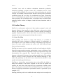
2.1 ASIP Design Flow
ASIP design is different from general hardware designs such as memory
design and general purpose processor design. ASIP design starts with an
explicit application behavior study. Because ASIP core is designed to run
software with similarity, engineers can use the application to optimize the
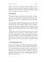
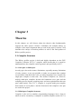
hardware by instruction set design. Figure 2.1 shows ASIP design flow.
There are five essential steps of ASIP design process.
Profiling: Starting with applications and design constraints as input,
profiling gives the engineer an overall view of the target product. The most
important role profiling phase provides is to expose the structure of the
application, finding the part of the application which could possibly
becoming bottleneck when implementing on hardware. Applications, which
are written in high level languages, are analyzed statically and dynamically
and the result is stored in appropriate intermediate representation, which is
Background and Previous Works
Chapter 2
used in subsequent steps.
Applications
and Design
Constraints
Profiling
Architectural
Design Space
Exploration
Instruction
Set Design
Benchmarking
Hardware
Implementation
Software
Design and
Testing
Figure 2.1 ASIP Design Flow
Architectural Design Space Exploration: several suitable architectures are
selected for the specified applications by using profiling result and design
constraints. The final decision goes to the architecture that satisfies both
estimated performance and power requirements with lowest possible
hardware cost.
3
Background and Previous Works
Chapter 2
Instruction-set Design: With the result of profiling, instruction set is
synthesized for the particular application and select architecture. [17] The
instruction set guides hardware design as well as software design.
Hardware Implementation: Hardware is built under the selected
architecture using ASIP architectural template to fulfill instruction set design.
Hardware and instruction set are written in description languages such as
VHDL or Verlog.
Software Design and Test: Application designed and optimized for the
particular hardware architecture is designed and synthesized. Special
designed instructions are used in the application. And after all the system is
tested and put on the market.
2.2 Hardware/Software Co-Design
As we can see from here, ASIP design is highly dependent on an interlaced
process of cooperated software and hardware design, so called
Hardware-Software co-design. Hardware-software co-design, or HW/SW
co-synthesis, simultaneously designs the software architecture of an
application and the hardware on which that software is executed. [5] [6]
Each hardware design phase is constrained by application requirements.
Design of additional software tools is also required during the design
process. [16] For example, in the final stage, a re-targetable special designed
compiler is needed to compile the high level programming language code,
in order to fit to the special designed hardware instruction set.
2.3 Previous Works
The profiler project is based on the research of Björn Skoglund’s Relief
profiler. The Relief profiler is focused on finding basic blocks that can
possibly be implemented into instructions. It analyzes the execution time of
each basic block and operations each basic block has to give suggestions for
instruction set design. More information about Relief profiler is introduced
in Chapter 4.1.
4
Chapter 3
Theories
In this chapter we will discuss about the theories that fundamentally
supports the entire project. Section 1 introduces the compiler theory, as
compiler is the major component that we used in the project. Section 2 will
introduce the concept of modern profilers as well as the final product of
Rilievo profiler project.
3.1 Compiler Structure
The Rilievo profiler project is built and highly dependent on the GNU
Compiler Collection (GCC) C compiler, which means that it is crucial to
understand how the compiler works in general, and specifically in GCC.
3.1.1 One-pass or Multi-pass
At early ages, due to the resource limitations, especially memory limitations
of early systems, it was not possible to make one program that contains
several phases and did all the work. So many languages were compiled by
single-pass compiler at that time. The modern compilers are, however,
majorly multi-pass compilers because the limitations were gone and the
compiling process became requiring more and more optimizations that one
pass cannot satisfy. The GCC C compiler is a typical multi-pass compiler
that consists of seven phases. And the front-end of the compiler is the part
we used in the project.
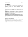
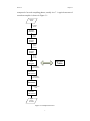
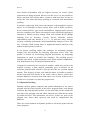
3.1.2 Multi-pass Compiler Structure
Compiler is the tool to translate programming languages into a form in
which it can be executed by a computer. A modern compiler such as GCC is
Theories
Chapter 3
composed of several compiling phases, usually 6 or 7. A typical structure of
a modern compiler is shown in Figure 3.1.
Source
Code
Character
Stream
Lexical
Analyzer
(Scanner)
Token
Stream
Syntax
Analyzer
(Parser)
Abstract
Syntax
Tree AST
Semantic
Analyzer
(Parser)
Abstract
Syntax
Tree AST
Intermediate
Code
Generator
Symbol
Table
Intermediate
Representation
Machine
Independent
Code Optimizer
Intermediate
Representation
Code
Generator
Target Machine
Code
Machine
Dependent
Code Optimizer
Target
Machine
Executable
Figure 3.1 Compiler Structure
7
Theories
Chapter 3
3.1.2.1 Compiler Front-End
Lexical Analyzer is the first phase of the entire compiler workflow. It is
also called the Scanner. The lexical analyzer reads character stream of
source code and groups the stream into sequences called lexemes, in which
tokens are generated. A token usually looks like <name, value >. The “name”
here is already not the same as in the source code character stream. It has
been replaced with a recognizable identifier which is located in the Symbol
Table. For example, after lexical analysis, a simple C program line
CODE
energy = matter * squal(speedOfLight);
will be transformed into
CODE
<var,1><=><var,2><*><func,1><(><var,3><)><;>
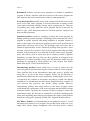
Syntax Analyzer is also called parser. It follows right after the scanner,
taking the token stream as input. The parser transforms tokens into a
tree-like intermediate representation that depicts the grammatical structure
of the token stream. A typical representation is an abstract syntax tree in
which each interior node represents an operation and the children of the
node represent the arguments of the operation. A sample tree of the C
program above looks like this:
=
<var,1>
*
<var,2>
<func,1>
arg_list
<var,3>
Figure 3. 2 Abstract Syntax Tree Example
8
Theories
Chapter 3
Semantic Analyzer uses the syntax tree and the information in the symbol
table to check the source program for semantic consistency within language
definition. It also gathers type data and stores it in both AST and the symbol
table that will be used by the intermediate code generator later. The output
of the semantic analyzer in GCC is the source we used in this project.
The three phases above are usually called the Front End of the compiler
together. GCC produces GENERIC trees as a complimentary of abstract
syntax tree as the final output of the front-end. For other compilers,
front-end usually has the similar functionalities as lexical analysis,
preprocessing, syntax analysis and semantic analysis and produces
intermediate representation as the output. The compiler front-end also
manages the symbol table which will be introduced later.
3.1.2.2 Compiler Middle-End
Intermediate Code Generator generates an explicit low level or machine
like intermediate representation, which can be treated as a program for an
abstract machine. With this intermediate representation, it is easy to
translate it into different target machine, which makes cross target compiling
possible in one compiler. In GCC, after the Abstracted Syntax Tree is
generated, a GIMPLE tree is generated by gimplify_function_tree() function.
The GIMPLE intermediate representation unifies all language front-end
GCC has so that there will be no more language dependent information later
on for target machine code generation.
Machine Independent Code Optimizer attempts to improve the
intermediate code so that better target code will result. The word “better”
here usually means target code that runs faster. But on certain applications
the optimizer would focus on other field such as lower power consumption,
less memory usage or shorter code. In GCC, an optimized intermediate
representation is called Register Transfer Language (RTL), which represents
an abstract machine with an infinite number of registers.
The two phases above are called the Middle End. Comparing to compiler
front-end and back-end, the middle-end is more ambiguous. The input of the
middle-end is intermediate representation, which is interestingly the same as
the output of middle-end. However the intermediate representation itself has
hugely changed either by form or by the functionality. For a simple compiler,
the middle-end may be integrated with other phases so it doesn’t exist
separately. But for most modern compilers that require more optimization
processes such as GCC, the middle-end is indispensible.
3.1.2.3 Compiler Back-End
9
Theories
Chapter 3
Code Generator is sometimes the last phase of the compiler. But it is
usually followed with code optimizer. The input that code generator takes is
the intermediate representation of the source program. Code generator maps
the input into the target language. The target language can be machine code
or assembly code. The generator allocates memory unit and register files for
the variables that defined and used in the source program. Then it translates
the sequential code of the intermediate representation into machine
instructions that perform the same functionality.
The term back-end is sometimes confused with code generator itself
because of the overlapped functionality of generating code. Some compilers
can also perform target machine-dependent binary code optimization, which
distinguishes the back-end out of the code generator.
For most compilers the front-end and the back-end are unique so that they
only compile one programming language on one target machine. For some
other compilers, such as GCC, they has various front-end that produces the
same intermediated code which accepted by the unique 1, machine dependent
back-end. These compilers however, can compile several programming
languages on the same target machine.
3.1.2.4 Symbol Table, an Important Compiler Component
Symbol table is a data structure which stores all the symbols and attributes
that relates to each one of the symbols. Those attributes identify the storage
allocations, types, scopes and other information of the symbol. Each
variable has a record in the symbol table in which it stores attributes of the
symbol in the corresponding scope. The data structure is designed to allow
each compiling phase to find the record for each variable quickly and to
store and retrieve data in and from that record quickly.
3.1.3 GCC as a Component
The profiler uses the GCC front-end to extract information from Control
Flow Graph that compiler generates. The information is syntax tree we
mentioned before. These trees are grouped by and accessed through a
structure which is called Basic Block. GCC C compiler breaks the source
program into basic blocks so the profiler itself has no need to take the job of
identifying them.
1
The word “unique” here means that you have only one back-end on the same set-up. However GCC
also supports cross-platform compiling with more back-ends.
10
Theories
Chapter 3
3.1.3.1 Control Flow Graph
Control Flow Graph (CFG) in general is a graphical representation of the
paths that might be traversed through a program during execution [12]. In
GCC however, a CFG is a data structure built on top of the intermediate
code representation, abstracting the control flow behavior of a function that
is being compiled. The intermediate representations are the RTL or tree
instruction stream. [13][14]
The CFG is a directed graph where the vertices represent basic blocks and
edges represent possible transfer of control flow from one basic block to
another. [18] The CFG we used in the project is built upon syntax trees and
traversed by FOR_EACH_BB macro. However because of the strict rules
that GCC has on trees in the CFG, tree representations cannot be easily used
or maintained without proper maintenance of the CFG simultaneously.
3.1.3.2 Basic Block
Basic blocks are the maximal sequences of instructions that are always
executed sequentially. Base on this, basic blocks has the properties that
(i)
The first statement of the basic block is and will always be the first
statement in the basic block execution flow. It is the only entry that
basic block has. There are no jumps into the middle of the basic
block.
(ii)
Once the flow enters into the basic block, the flow will not halt or
branch inside the block. Exceptions are only acceptable at the last
statement of the block [7]
Basic blocks are usually the basic unit to which compiler optimizations are
applied. The profiler gathers information of each basic block extracted from
the CFG and disintegrates them into statements to identify loops. Loop
identification is base on the fact that the first statement of each basic block
is a Label and there are no other Labels within the scope of basic block. [8]
More details of how the profiler identifies loops from the source program
will be introduced in Chapter 5.
3.1.3.3 Basic Block Overhead
Basic block overhead, or loop overhead, is a special feature our profiler
provides for boosting program execution speed. As we mentioned before,
basic block is consist of sequences of instructions that are always executed
together. However these instructions are the “visible” ones that are written
in the source code. The hardware cost of an ASIP processor also includes
11
Theories
Chapter 3
“invisible” ones such as address calculation, instruction prediction,
instruction pipelining, program counter (PC) calculation and etc. Loop
overhead is the additional cost of processor clock while taking the decision
of loops. For example, some processors needs 20 clock cycles to perform a
conditional jump and even more for conditional long jump. Abstracting
these overheads makes the profiler toolset more precise while analyzing the
source program. We will introduce how to configure these overheads while
using the profiler toolset in Chapter 4 and how these functions work in
Chapter 5.
3.2 Profiler Theory
Profiler is a performance analysis tool that analyzes program’s static and
dynamic behavior. Static profiler is also called static code analyzer which
analyzes the behavior of computer software without actually executing the
program. Dynamic profiler on the other hand, is performed by executing
program and traces certain properties during the execution.
3.2.1 Static Profiling
Static profiling, also known as static code analysis, is a method of
measuring the source program in different aspects of performance by
traversing the source code without executing it. Depending on the aspects it
focuses on, static profiler analyzes the source code from different depth,
forms and representations.
Profiling on source code is an approach similar to lexical analysis which is
focused on aspects such as memory optimization or type verification. Code
is the direct output from the programmer in which it represents the logic and
functionalities the program has. Especially high level programming
language is designed for human to better understand the logics. The machine
however, finds it is hard to interpret the code without compiling it. This
makes the granularity on this level is too coarse that the profiler is only
capable to identify superficial issues.
Profiling on intermediate representations gives the profiler the ability to
analyze the structure of the source program. In this case the profiler can
optimize the work flow of the program or give suggestions of which certain
part of the program consumes the most hardware resource. Our project is
based on analyzing intermediate representation which is generated by the
compiler. [15]
Profiling on binary code level enables the static analysis tool to analyze the
12
Theories
Chapter 3
most detailed information with the highest accuracy on exactly which
instructions are being executed. However on this level, it is not possible to
follow structural flow which makes it hard to make decisions on how to
resolve the issue unless the binary profiling is connected with intermediate
profiling.
In software engineering field, static code analysis is often applied in security
aspect. It is a technique to detect security holes, such as buffer overflows,
access control policies, type based vulnerabilities, language-based security
and even computer virus. Static code analysis works with model checking or
templates to identify security leakage. Such tools includes RATS (Rough
Auditing Tool for Security), Coverity Prevent (identifies security
vulnerabilities and code defects in C, C++, C# and Java code), Parasoft
(security, reliability, performance and maintainability analysis of Java, JSP,
etc.), Veracode (finds security flaws in application binaries and byte code
without requiring source), and etc.
In our project, profiling implies the technique for estimating program
running cost and payloads by analyzing application source code. Our
profiler is focused on accelerating program performance by integrating
instructions as much as possible into hardware. The profiling process
includes basic block weight calculation, basic block payload computation,
loop identification, loop overhead calculation and etc.
Compared to monitoring an execution at runtime, which may not have the
required coverage, a static analysis potentially gives an analysis on all
execution paths possible instead of just the ones that are executed during
runtime. This property of static code analysis makes it possible to analyze
all the loops and basic blocks in the source code to observe which ones
consume hardware resources more than others even if some of those won’t
be able to be executed every time the program runs.
3.2.2 Dynamic Profiling
Dynamic analysis gathers temporal and spatial information of the source
program from pre-placed probes in the source program binary code during
execution. By using dynamic profiler, we can easily find out how much time
each part of the program used and which functions are called that are made
by branch decision. This information can tell us if there are parts of the
program runs slower than expected, and could be implemented into
hardware.
There are several methods for dynamic profiler to release the probes into the
source program.
13
Theories
Chapter 3
Benchmark software uses the source program as a module or standalone
program. It doesn’t interfere with the execution of the source program but
only measures the total execution time it takes or other parameters.
Event based profilers usually works with a framework which exists on the
lower level of the source program. It uses the framework to capture certain
events such as function entering, leaving, object creation and etc. This type
of profiling only works while the source program has the framework on
which it runs. .NET framework and Java VM both provides interfaces for
those profiling functions.
Statistical profilers operate by sampling. It probes the source program by
adding operating system interrupts. Sampling profiler interrupts the source
program at regular intervals and taking snapshots of program counter or
stack or other fields. This allows the program to run at a near practical speed
without have efficiency loss or lags. The profiling result is not exact, but a
statistical approximation. In fact, statistical profiling often provides a more
accurate result of the execution of the source program than other profiling
methods. And because there is no insertion of probes on the source program,
fewer side effects, such as cache miss due to memory reload or pipeline
disturbing, are made this way. However these profilers need support from
hardware level which basically means only the hardware maker has the
possibility to implement it. Such profilers are Code Analyst from AMD,
Shark from Apple, VTune from Intel and etc.
Instrumenting profilers injects small pieces of code as probes into the
source program to perform observing the runtime behavior of the program.
These profilers have fewer dependencies than other types of profiler and
acting like it is part of the source program. Probes can be manually or
automatically added into the source program by modifying the source code,
or assisted by the compiler to add probes according to certain rules during
compilation, or instrumented into the binaries that produced by compiler, or
even injected into processes and threads during runtime. However
instrumenting profilers also brings defects to the source program which
could change the performance of the source program and potentially causing
inaccurate results. Typically, the execution of source program is slowed by
instrumented codes but this can be optimized by carefully choosing probe
points and controlling their behavior to minimize the impact. Such profilers
include the GNU gprof, Quantify, ATOM, PIN, Valgrind, DynInst and etc.
The Rilievo Profiler uses instrumenting as the method to observe, record
and analyze the behavior of a program. Our profiler insert probes on every
single basic blocks during compilation time and these probes collects
14
Theories
Chapter 3
runtime information for the analyzer to identify runtime loops. Due to the
fact that the probes generates extra codes and occupies extra memory space,
the execution takes more time than it normally does.
Dynamic profiling can observe certain properties of a program that static
analysis is hard or even impossible to notice. Dynamic profiling collects
runtime execution data that cannot be analyzed without execution.
In the next chapter, we will introduce you how to use both static and
dynamic profilers in our toolset and the chapter after will introduce you
what the architecture of this toolset and how these tools are designed.
15
Chapter 4
User Manual
The previous chapters introduced what an ASIP profiler is and how it works.
In this chapter, we will introduce the Rilievo profiler and how to get it
working. This chapter will also introduce you the Rilievo Analyzer which
analyzes the outcome from the profiler. The implementation of the profiler
and the analyzer will be introduced in Chapter 5. Section 4.2 introduces the
workflow of the software. Section 4.3 to 4.5 will guide user through the
installation and configuration process.
4.1 The Rilievo Profiler and Relief Profiler
As we mentioned in Chapter 2.3, the Rilievo profiler is developed based on
Björn Skoglund’s Relief profiler. The main purpose of Relief profiler is to
observe basic block execution to see if optimizations can be made by
reducing it. In his design, the profiler extracts basic block information and
writes them into an xml file. The xml file is then used by graphical
analyzers. In the new design, we want to keep this xml file and the
information it contains. Moreover, as what we are mainly interested in is
that how the program can be optimized by eliminating loops, the Rilievo
profiler will also extract loops from the source program to another xml file,
which will be analyzed by the analyzer. The Rilievo profiler also accepts
configuration file which defines the weight of each operations, so that the
estimation of application payload will be even more precise. Information
about how to use these files will be introduced later. The word “profiler” in
this paper, if not particularly specified, would refer to the Rilievo profiler.
User Manual
Chapter 4
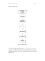
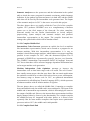
4.2 Workflow Overview
The profiler is developed under UNIX compatible operating system so that
you may run the profiler almost everywhere. Base on this, the workflow can
be divided into three steps.
Compile
customer
software
Compile the
profiler
Analyze the
result
Figure 4.1 User Workflow
4.2.1 Compile the Profiler
In this step, users need to configure the profiler library and compile it using
the latest GCC. Because the profiler is based on GCC 4.1.0/GEM 1.7, it is
recommended to use higher GCC version than 4.1.0 to compile the profiler.
The compilation process will be similar to compilation process of GCC
4.1.0.
4.2.2 Compile the Software
Here the user compiles the customized software by using freshly built
Rilievo profiler with GEM extension linked. In this step, the Rilievo profiler
will read configuration file and process the source program eventually
produce xml files and executables. The executables are linked with dynamic
profiler library and is ready to use. The executable can be either called by
other program or executed by itself and runtime information will be save to
other xml files.
4.2.3 Analyze the Result
With the xml files produced previously, user can use Java based Rilievo
Analyzer to observe the structure of the program. Find out which part of the
program executed the most and which loops are the most executed loops.
4.3 Installations– Compile the Profiler
4.3.1 System Requirement
UNIX compatible OS is required, e.g. Linux, Mac OS, BSD, Solaris, etc.
The previous Relief profiler is “developed on a PC running Gentoo
linux-x86-64”. And the Rilievo profiler is developed on several Linux
17
User Manual
Chapter 4
distributions, including RHEL Centos, Debian Ubuntu and Solaris. We
cannot guaranty that the Rilievo profiler will run on every Linux distribution
but with more or less effort it will probably run on which there contains an
official release of GCC. It is also recommended to use a 32-bit system
because compiling GCC with 64/32 mixed libraries would introduce
problems.
GCC C-compiler is the foundation of the profiler. GCC is the GNU
Compiler Collection of which C compiler is mainly used. GCC is bundled
with most Linux/UNIX/BSD distributions and can be easily found on GNU
http://gcc.gnu.org website.
GEM Framework is GCC extension modules developed by State
University of New York. With GEM user can dynamically change the
behavior of the compiler without re-compiling it. About what a GCC
extension is will be explained in the next chapter. GEM can be downloaded
via svn site.
Miscellaneous A complete installation of the Rilievo profiler requires
certain existed software. Some of these pieces of software are pre-installed
in the system depending on the Linux distribution it is built on. Known
software is FLEX, a fast lexical analyzer, and BISON, a GNU parser
generator.
4.3.2 Step-by-step Installation
4.3.2.1 Download GEM
The latest version of GEM (the Rilievo profiler is built on version 1.7) can
be found on http://www.ecsl.cs.sunysb.edu/gem/ Download and extract the
first item, gem1.7.tar.gz, in “Installation” field. Most modern Linux
distributions include GUIed file extractor such as “file-roller”. You can also
use the command below to untar the file.
CODE
user@machine: $tar xzf gem1.7.tar.gz
4.3.2.2 Configure GEM
After the extraction, use any text editor to open the Makefile, which is
located in folder gem-1.7. Modify the first two lines to the following.
CODE
#GCC_RELEASE=3.4.1
18
User Manual
Chapter 4
GCC_RELEASE=4.1.0
Please be noticed that the GCC used here is version 4.1.0.
Then change the source download address of GCC to the following if you
are in Sweden.
CODE
wget
--passive-ftpftp://ftp.sunet.se/pub/gnu/gcc/releases/gcc-$(GCC_RELEASE)/
gcc-core -$(GCC_RELEASE).tar.gz;\
4.3.2.3 Download and Patch GCC
Now you will have the GEM package available. To download GCC, simply
use the command
CODE
user@machine:~/gem-1.7$make gcc-download
This will download, extract and patch GCC. If the downloading is too slow,
please find a server near you on http://www.gnu.org/prep/ftp.html and change
the download address mentioned before according to the rule then start over
again.
The gcc-download command will patch GCC with GEM as well. The
following command will help patching GCC iff patching fails during
gcc-download.
CODE
user@machine:~/gem-1.7$cd gcc-4.1.0
user@machine:~/gem-1.7/gcc-4.1.0$patch –p2 < ../patch/gem-4.1.0.patch
4.3.2.4 Compile GCC
Once GCC is successfully patched, you may start to compile it. Change the
working directory to gem-1.7 and use make command to start compilation.
CODE
user@machine:~/gem-1.7$make gcc-compile
If make directly, the Makefile will invoke both gcc-download and
19
User Manual
Chapter 4
gcc-compile. It is recommended to do it separately because mistakes can be
made and neglected. In this case, however, make will ignore gcc-download
but compile GCC only.
The Makefile script also includes installation of the fresh compiled GCC. It
is not recommended to do so since this would possibly affect the
compilation of other software. The compilation of GCC would most likely
to take quite a few minutes or up to hours depending on the speed of the
machine. Although the process could be interrupted by errors or restrictions
of the system, it usually works fine if an un-patched GCC can be normally
and manually installed in the system. However if it doesn’t, you might need
to solve it before having more problem with the patched GCC later.
Solutions to general compiler installation problems can be easily found on
the internet.
After the compilation, if everything works fine, we will have a fully
functioning patched GCC. We will then use it to compile our Rilievo library.
4.3.2.5 Download the Profiler Library
The project is located on svn server of ISY. One might need authorizations
in order to access these files. The following command will retrieve the
profiler library from the server.
CODE
user@machine:~/gem-1.7$svn co https://svn.isy.liu.se/daxjobb/rilievo rilievo 1
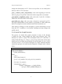
4.3.2.6 Build the Profiler
Before build the profiler library, a few configurations are needed due to
different environment variables on different systems. The entire Rilievo
profiler consists of four components distributed in five folders: Java
Analyzer, Instrumenter, Profiler, Util and test. Each one except the Java
Analyzer has a Makefile in it. Use any text editor to open the Makefile and
change the CC variable to the path of the executable binary of the patched
GCC according to your compilation. Below is one example of the
configuration.
CODE
CC = ~/gem-1.7/gcc-4.1.0/bin/bin/gcc–I../util/
1
The name of the folder could be different due to maintenance of the svn server.
20
User Manual
Chapter 4
Also, open the Makefile.conf in instrumenter folder and change the variable
GCC_BASE to the absolute path of where the patched GCC exists. Please
be noticed that you cannot use relative path for this variable. For example,
CODE
GCC_BASE=/home/user/gem-1.7/gcc-4.1.0
Modify the INCLUDE variable to fit the architecture of the system you are
using.
CODE
INCLUDE=-I.
-I$(GCC_BASE)/gcc
–I$(GCC_BASE)/include
–I$(GCC_BASE)/gcc/config
–I$(GCC_BASE) /host-i686-pc-linux-gnu/gcc –I$(GCC_BASE)/libcpp/include
To build the Rilievo profiler library, simply use make command in each
component folder. A recommended order would be Util, Instrumenter and
then Profiler. To be noticed, the Instrumenter needs bison and flex to
compile so please be sure they are installed in the system before the
compilation. After the compilation, a file named “ci.gem” will be available
in bin folder of Instrumenter. This file is the GEM extension that is going to
be used later.
4.4 Compile Customer Software
4.4.1 System Requirement
There is no specific requirement other than the ones mentioned before. If the
profiler can be compiled in the system, it should also compile customer
software.
4.4.2 Regular Compilation
In the folder called “test”, there are a few sample customer programs wrote
for demonstration. Once the compilation of the profiler itself is done, the
user can use the following command as an example to compile the customer
software with GEM extension.
CODE
user@machine:~/UserSoftware$~/gem-1.7/gcc-4.1.0/gcc/bin/bin/gcc
-fextension-module=~/gem-1.7/rilievo/instrumenter/bin/ci.gem
–L~/gem-1.7/rilievo/profiler –lprofile YourProgram.c
21
User Manual
Chapter 4
The compilation command essentially contains three different parts.
(i)
First make sure you are using the fresh built custom GCC instead of
GCC which is not patched to compile the software.
(ii)
Second, the patched GCC would take the “ci.gem” file built by the
instrumenter library as the extension to perform the hooks and GCC
hacks during the compilation. Here the user should include the path
of the extension file. The patched GCC would function no more than
a normal GCC if the extension is not used.
(iii)
The customer software needs to be statically linked to the profiler
library. Therefore the path of the profiler library should be included
by adding argument “-L”.
The automatic build script Makefile is also available in the test folder, where
users can make their own build script regarding to the rules above. The
existing Makefile contains compile command to three demonstrative
programs which can be used as examples.
The compilation in this step would actually generate both static data, which
is in the form of several xml files, and executables. The Rilievo Analyzer
can analyze the static data without any need to execute the software. The
executables on the other hand, are instrumented with dynamic profiling
ability that generates data during runtime.
4.4.3 Opt-in Compilation
In order to make the profiler work more precisely, a configuration file is
needed to specify the processor clock cycle each operation would take. For
example an ordinary add in the pipe line costs one clock cycle of the
processor while a division normally costs 20. Ignoring these huge
differences would dramatically change the profiling focus. In the Rilievo
profiler, this clock cycle preference is called “weight” and stored in a
configuration file. Each program that is going to be profiled should have a
configuration file name after the program. A sample configuration file could
look like this.
CODE
add 1
mul 2
div 20
bbo 3
22
User Manual
Chapter 4
Each line in the file represents for one entry that consists one key and one
value, separated by a space. The key is the mathematical function that needs
to be weighted. It is limited to three letters’ abbreviation. The value is the
processor clock cycle the responding mathematical function needs to
perform. The mathematical functions it supports includes but not limited to
basic mathematical functions such as arithmetic, bitwise operation,
comparisons and so on. Also customer defined algorithm can be weighted
by the profiler but this requires modifying the profiler itself. This will be
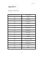
explained in the next chapter. A table of supported pre-defined operator keys
is attached as Appendix A.
If the configuration file is not given during the compilation, the profiler will
take 1 as the weight factor for all the operators. To be noticed that the “bbo”,
a.k.a. basic block overhead that we mentioned in last chapter in this case
would be set to one as well instead of zero, which means there’s always
some overhead during execution
Once the compilation is done, the profiler will generate two xml files and
one graph file. The “filename.c.stat.xml” file contains computational
payload information of basic blocks while the “filename.c.path.xml” file
contains structural information of the program. The graph file can be used to
draw program flow graph. More about the graph file will be introduced in
the next chapter. If the user chooses to execute the instrumented software,
several dynamic profiling xml files will be generated. They are named as
“filename-PID.dyn.xml” and “filename-PID.log.xml”.
4.5 Analyze the Result
4.5.1 System Requirement
Despite the requirements before, a working Java VM is also needed. Most
Linux Distributions includes or can be installed with Java Runtime
Environment (JRE). The latest JRE package is available on
SUN/ORACLE’s website. It is recommended to install JRE from
distribution independent software repositories, e.g. Synaptic in Ubuntu. The
Rilievo Analyzer can also run on most Windows machines because Java is
platform independent.
4.5.2 Analyzer Walk-Through
As shown in the workflow graph previously, this step is the last step of the
entire flow. From the previous steps, the profiler has generated two xml files.
Here we need to use the Rilievo Analyzer to analyze them.
23
User Manual
Chapter 4
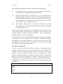
The graphical interface of Rilievo Analyzer looks like this.
Figure 4.2 User Interface of Rilievo Analyzer
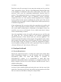
Click on File menu and choose open, or use keyboard shortcut “Ctrl + O” to
open “Open File” dialog. And choose the file generated by profiler
“filename.c.path.xml”. Choose the one named after executable if you have
multiple files in the project or any of those if you want to see static analyze
result for that file. Please notice that the file used here is the path file.
Figure 4.3 Open File Dialog. It’s OS dependent so the UI should be consistent with the system
24
User Manual
Chapter 4
Now you need to choose whether you’d like to perform a static analyze or a
dynamic one. When choose “dynamic”, the user also needs to choose a
“runtime” file which specifically associated to a single execution.
Figure 4.4 Mode Selection Dialog
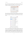
Here you have the main window of the static analyzer if you chose “static
mode” in the last step. On the left side is the working flow of the program
while on the right side is information associated to the blocks or loops on
the left.
Figure 4. 5 Program’s Main Window Frame
The user can select the blocks on the left window. The blocks marked as red
text are the Labels of the program. It is automatically generated by profiler
to observe the working flow of the program. The BBs are basic blocks. A
function can be divided into several basic blocks with same prefix. The blue
blocks are loop labels. In each loop label it shows which label the loop goes
back to. The user can click on basic block and loop blocks to inquire more
25
User Manual
Chapter 4
information. The label blocks however are not responding to user
commands.
The upper right box shows general information of the selected block or
blocks. It shows the name and line number of the source code of the selected
block when the selection is made on basic block. It also shows what
operators the basic block contains. When click on loops on the left side, the
upper right box would show the start basic block and the end basic block
and their location in the source code of the selected loop.
The lower right box, on the other hand, shows the payload of the selected
basic block or loop. It shows three kinds of information of basic blocks: i)
payload of the selected basic block, ii) exact payload of the selected basic
block while in loop, iii) times that basic block will be executed. When
clicking on loop blocks, this box will show the computational payload that
entire loop has, and the number of basic blocks and inner loops that loop
has.
Particularly, when the user click on the loop blocks on the left, the entire
loop will be highlighted to inform the user where the loop locates
graphically. As shown below.
Figure 4.6 Loop Selection
Through the menu “statistics”, user has the access to two statistical result of
26
User Manual
Chapter 4
the source program: the most executed basic block and the heaviest loaded
loop. User can use this result to optimize the ASIP processor by building
these pieces of code into hardware.
If the user selected “dynamic mode” in the profiling mode selection dialog
(Figure 4.4), on the other hand, the analyzer will open up another “open file”
window to ask the user to select a dynamic loop analysis file. To generate
this file, the user needs to run the customer software successfully. After a
single execution, the dynamic profiler will generate a dynamic loop analysis
file. The naming rule for this file is “program_name-PID.log.xml”, in which
“PID” is the process id of the execution.
When the dynamic loop analysis file is selected, the analyzer will list all
loops identified during selected execution. If click on the items on the left
window frame, the analyzer will show statistic data of the selected loop on
the right frame, including basic block list, inner loop list and clock cycle
count.
Figure 4.7 Dynamic Analysis GUI
27
Chapter 5
Design and Implementation
We have discussed how to use the tool in the last chapter. In this chapter, we
will discuss how we designed and implemented the Rilievo profiler toolset.
Section 5.1 will introduce workflow of the toolset. Section 5.2 and 5.3 will
explain how static and dynamic profiler works in detail.
5.1 Software Architecture
5.1.1 Architecture Overview
To begin with, we would like to introduce the architecture of our profiler. As
we mentioned before, the Rilievo profiler can be divided into 3 components:
the static profiler, the dynamic profiler and the analyzer. The static profiler
and the dynamic profiler are developed based on GCC 4.1.0 and GEM 1.7
while the analyzer is developed using Java technology. The workflow as we
introduced in the previous chapter can be divided into three parts too:
compiling the profiler, compiling customer software and analyze the result.
Compile the profiler
Patched GCC + Profiler Lib.
Profiler GCC Extension
Compile and run customer software
Profiler GCC Extension
XML Data
Analyze the result
XML Data
Visual Feedback
Figure 5.1 Profiler Workflow (steps, input and output of each step)
Design and Implementation
Chapter 5
It starts with a patched GCC is compiled and is used to compile the profiler
libraries. Then the profiler libraries are used to compile customer software
to generate statistical result. With the result, an analyzer is then used to
analyze and give user graphical feedback. In brief, the profiler uses a
patched GCC as a part of it and generates information for the analyzer to
show to the user. The graph shown above demonstrated the input and output
of each step in the workflow.
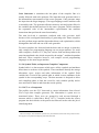
5.1.2 Profiler Workflow
In the last section, we mentioned that the Rilievo profiler takes the patched
GCC as a part of it. The figure below illustrated the work flow graph of
GCC interacting with our profiler.
User
Software
Lexical
Analyzer
(Scanner)
Compiler Front End
Tokens
Syntax
Analyzer
(Parser)
Abstract
Syntax
Tree AST
Rilievo Profiler Toolset
Semantic
Analyzer
(Parser)
Abstract
Syntax
Tree AST
CFG Tree
Generation
CFG Tree
Element
Extrator
Basic
Block
Data
Source Code
Optimizer
(Intermediate
Code Generator)
Loop
Analyze
Data
Loop
Analyze
Analyze
Result
Compiler
Backend
Figure 5.2 Profiler Workflow
29
Design and Implementation
Chapter 5
The source program is scanned and parsed by GCC C-compiler as we
introduced in Chapter 3. After that, the compiler front-end generates CFG,
the Control Flow Graph, and fed to the instrumenter component. Among the
two kinds of representation that GCC has, which are RTL and tree
instruction stream, here in the Rilievo profiler, we use the tree representation
of the CFG to extract basic block and loop information. Details on how the
profiler extracts all the information we need will be explained later. As we
can see from the graph, CFG is the key to connect GCC and our profiler.
And only with GEM can we have the possibility to access kernel functions
of GCC.
5.2 Static Profiler Library
The main components of Rilievo profiler are the static profiler, dynamic
profiler and the analyzer. In this section, we will discuss the static profiler
library and how they are implemented in detail. The product of each step
will also be demonstrated in this section.
The static profiler library is located in the folder called “instrumenter”. A
brief file list is attached at the end of this section. From Figure 5.2 we can
see that the bridge that connects GCC flow and the profiler is the CFG tree
extraction and this is what the static profiling library is responsible for.
5.2.1 GEM: the GCC Extension Modules
GCC is an open-source compiler that all the source code is available under
GNU/GPL license, which means that everyone has the access to the source
code and has the opportunity to modify GCC for better security,
dependability, and others. An extension of GCC is normally done by
modifying the source code of the compiler directly. This design is weak on
version control because when the end user needs to use different versions of
extension, he needs to download all the specialized compilers separately and
build them together. What makes it worse is that if he wants to publish this
combination even without modifying anything, he will have to publish it as
another different version. The GEM framework is developed under this
circumstance. “The goal of this project is to create a framework for writing
compiler extensions as dynamically loaded modules.”“With GEM the
developers need to distribute the source code of the compiler extension only.
The GEM-patched compiler loads at run time a GEM module specified as
the arguments of its –fextension-module option.” [9] In a word, instead of
building extra versions of GCC, user can publish the extension file only.
In GEM there are a bunch of hooks that inserted into GCC enables us to
30
Design and Implementation
Chapter 5
change the functionality of GCC. Here in our profiler, we use mainly three
hooks to achieve CFG extraction.
gem_c_common_nodes_and_builtins(): calls at the beginning of each file
which is going to be profiled. In this hook all the output files are initiated.
gem_finalize_compilation_unit(): calls at the end of each file. It flushes
output files and writes them on the storage.
gem_build_tree_cfg(): calls every time a function is processed by GCC.
The major functionalities of the profiler is performed or called within this
hook. For example tree node extraction, basic block extractions, etc.
These hooks in GEM give us the possibility to extract information we need
from the GCC workflow to our profiler, building necessary bridges the
profiler needs.
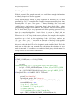
5.2.2 Control Flow Graph Extraction
The process of control flow graph extraction is done in the function
ci_build_tree_cfg(), which triggers the hook gem_build_tree_cfg(). The
function we used to extract CFG information from GCC data flow is
FOR_EACH_BB loop [11]. The for_each_bb loop will iterate all the basic
blocks one by one in the current function. In each iteration, we use a “block
statement iterator” [12] to traverse through every single statement and then
extract the operators we need from the statement. A sample code is shown
below.
CODE
FOR_EACH_BB(bb) {
if (filter_name(name)) {
break;
}else {
block_stmt_iterator si;
for (si = bsi_start(bb); !bsi_end_p(si); bsi_next(&si))
{
tree stmt = bsi_stmt(si);
if(lastIsLabel == true) {
if(TREE_CODE(stmt) == COND_EXPR) {
tree op0 = TREE_OPERAND(stmt, 0);
…
31
Design and Implementation
Chapter 5
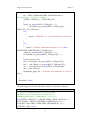
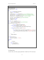
5.2.3 Loop Identification
With the control flow graph extracted, we would have enough information
to identify loops in the source program.
Loop identification is based on loop expansion in the form of CFG that
generated by GCC C-compiler. The compiler interprets possible loops into
assembly-like “if…goto…else…goto…” format, including “for” loops and
“while” loops. And because C program doesn’t have labels like in other
programming languages such as Basic, the compiler front-end creates labels
for it. Labels here play a very important role in the profiling process. Every
time the compiler identifies a basic block, it creates a label with an
identification number. This number is unique within the scale of a function.
When there is a “for” loop in the source program, for example, the compiler
would set up a label at the beginning of the “for” loop, and set up
“if…goto…else…goto…” tree node at the end of the loop with another
label. By extracting this special tree node and comparing the label IDs in
this node with the label ID of the beginning node and the label ID of the
node next to this node can we make the conclusion that whether this tree
node is a normal “if” condition or a conditional back jump, which means it’s
a loop. Pieces of code can be found below:
CODE
if(lastIsLabel == true)
{
if(TREE_CODE(stmt) == COND_EXPR)
{
tree op0;
//cond_expr[stmt]--->(k <= 3)[op0] goto L[op1] else goto L[op2]
tree op1 = TREE_OPERAND(stmt, 1);//here you get GOTO_EXPR
op0 = GOTO_DESTINATION (op1);//here you get LABEL_DECL
if(lastLabelUID > (int)LABEL_DECL_UID(op0))
{
printf("loop found!!\n");
fprintf(path_graph_file, "<loop>\n
<entry_point>%d</entry_point>\n", (int)LABEL_DECL_UID(op0));
currentBBIsLoop = true;
// e.g. k <= 3 goto Label
//1. extract "k <= 3" op0=k, op1=3
//2. find k in the list
//3. 3 is the limit of k, so write 3 into the list
op0 = TREE_OPERAND(TREE_OPERAND(stmt, 0),
32
Design and Implementation
Chapter 5
0);//cond_expr0--->le_expr0--->var_decl
op1 = TREE_OPERAND(TREE_OPERAND(stmt, 0),
1);//cond_expr0--->le_expr1--->integer
if(TREE_CODE(op1) == INTEGER_CST)
{
if(find_var_pos((int)DECL_UID(op0)) != -1)
varList[find_var_pos((int)DECL_UID(op0))][3] =
TREE_INT_CST_LOW(op1);
else
{
printf("** ERROR! **\n Cannot find the loop factor!\n");
}
}
else
{
printf("** Warning, unidentified variable %s. \n", (char*)
IDENTIFIER_POINTER(DECL_NAME(op1)));
if(find_var_pos((int)DECL_UID(op0)) != -1)
varList[find_var_pos((int)DECL_UID(op0))][3] = -1;
}
int start, end, inc, iters;
start = varList[find_var_pos((int)DECL_UID(op0))][1];
end = varList[find_var_pos((int)DECL_UID(op0))][3];
inc = varList[find_var_pos((int)DECL_UID(op0))][2];
iters = (end - start)/inc;
fprintf(path_graph_file, " <iterations>%d</iterations>\n</loop>\n",
iters);
}
}
lastIsLabel = false;
}
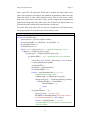
The following piece of code calculates number of iterations a loop has.
CODE
/* if op1 is +/- and operand 1 of op1 is var_decl and
operand 2 of op1 is integer then we consider op1 is
something more like: b + 2 rather than 2 + a or a - b */
elseif((TREE_CODE(op1) == MINUS_EXPR || TREE_CODE(op1) ==
PLUS_EXPR) ? (TREE_CODE(TREE_OPERAND(op1, 0)) ==
VAR_DECL && (TREE_CODE(TREE_OPERAND(op1, 1)) ==
INTEGER_CST)) : false)
33
Design and Implementation
Chapter 5
{
if((int)DECL_UID(op0) == (int)DECL_UID(TREE_OPERAND(op1,
0)))
{
// to-do: find the position of the UID in varList
//
edit the iterations field of the loop factor
//
if not found. make a new one. this happens
//
iff a var is used without initialization
//
// here we get something like "k = k + 1". so the only thing
// done here is to set the in/decrement value of k in the table
int decl_pos = find_var_pos((int)DECL_UID(op0));
if(decl_pos != -1)
{
if(TREE_CODE(op1) == PLUS_EXPR)
{
varList[decl_pos][2] =
TREE_INT_CST_LOW(TREE_OPERAND(op1, 1));
}
else
{
varList[decl_pos][2] = 0 TREE_INT_CST_LOW(TREE_OPERAND(op1, 1));
}
}
else//if the variable cannot be found, make a new one in the table
{
varList[currentListPos][0] = (int)DECL_UID(op0);
if(TREE_CODE(op1) == PLUS_EXPR)
{
varList[currentListPos][1] =
TREE_INT_CST_LOW(TREE_OPERAND(op1, 1));
varList[currentListPos][2] =
TREE_INT_CST_LOW(TREE_OPERAND(op1, 1));
}
else
{
varList[currentListPos][1] = 0 TREE_INT_CST_LOW(TREE_OPERAND(op1, 1));
varList[currentListPos][2] = 0 TREE_INT_CST_LOW(TREE_OPERAND(op1, 1));
34
Design and Implementation
Chapter 5
}
currentListPos++;
}
}
}
The identification process is done in “instrumenter.c” program. After the
identification, however, it is “static_analysis.c” that actually writes the flow
graph with loop identification information into “filename.c.path.xml” file. It
is done in this way simply because the program needs to maintain a variable
table during the process in order to be able to identify the number of
iterations of the loop.
In most ASIP programs, the number of iterations is usually explicitly
defined during the design phase. It is however possible to have implicitly
defined iterations or dynamically defined iterations. On those circumstances,
the iteration factor will be marked as “undefined” in the analyzer so that end
user will need to compute it manually.
5.2.4 Static Analysis I/O
Before the profiler processes the source program, it needs to read a
configuration file which contains processor clock cycle information of each
mathematical and custom function, known as “weight” file. The sample of
“weight” file is demonstrated in the previous chapter. Here we are going to
show you how the program stores and manipulates “weight”, as well as
basic block computational payload information.
In the static analysis program(“static_analysis.c”), the computational
payload information of each basic block and the processor clock cycle
information are stored in a C-structure called “bb_stat_def” which can be
found in “static_analysis.h” file.
CODE
struct bb_stat_def {
unsigned int mem_read;
unsigned int mem_write;
unsigned int func_call;
unsigned int division;
unsigned int bitwise_xor;
…
…
unsigned int basic_block_overhead;
35
Design and Implementation
Chapter 5
unsigned int total;
};
The processor clock cycle preference (“weight”) file is read during the
initiation process and stored in one of these structures. When the operators
are extracted from control flow, they are counted in another instance with
exactly the same structure. After processing of each basic block, these
structures are multiplied and finally write into the “.stat.xml” file.
However if the user wants to add custom weight factor, it is needed to
extend this structure and manually add resolve operations in the source file.
For example, if a function called “sin” is needed to be optimized, besides
adding corresponding line in the “bb_stat_def”structure, there are four
places that are needed to modify. The lines that are needed to be added are
included in the code below. It should apply to any custom functions.
CODE
void add_weight(bb_stat weight, char* bbsn, int w)
{
if(!strcmp(bbsn, "add"))
…
//add these lines below for extension of condition
else if(!strcmp(bbsn, "sin"))
{
weight->sin = w;
}
…
CODE
void sum_up_ops_with_weight(bb_stat stat, bb_stat weight) {
stat->total += stat->mem_read;
…
//add this line anywhere
stat->total += stat->sin;
…
36
Design and Implementation
Chapter 5
CODE
void analyze_tree(tree t, bb_stat stat) {
switch(TREE_CODE(t)) {
…
case FUNCTION_DECL:
//add the lines below, it works will all function calls
if((char *) IDENTIFIER_POINTER(DECL_NAME(t)) == "sin")
{stat->sin++};
break;
…
CODE
void output_weight_stat(char* bb_name, bb_stat stat, location_t* locus,
char* file_name) {
…
if(stat->min)
OUT(min);
//add the lines below
if(stat->sin)
OUT(sin);
There is so far no way to automatically has this done simply because the
program itself doesn’t have the access to its own source code to change the
structure. But as given above this would not be too complicated to achieve.
The user also needs to re-compile the static profiler after the modification.
The outputs of static analysis, as mentioned many times before, are two xml
files. The naming rule for both these files are “c_filename + .c + .(stat|path)
+ .xml”. Here are samples of these files.
CODE
<?xml version="1.0"?>
<stat_file>
<basic_block>
<name>func_0</name>
37
Design and Implementation
Chapter 5
<locus>
<file>simple.c</file>
<line>6</line>
</locus>
<stats>
<mem_read>2</mem_read>
<func_call>1</func_call>
<total>3</total>
<basic_block_overhead>0</basic_block_overhead>
</stats>
</basic_block>
<basic_block>
<name>main_0</name>
…
Sample file “simple.c.stat.xml”
CODE
<?xml version="1.0"?>
<loop_analysis>
<bb>func_0</bb>
<bb>main_0</bb>
<label>0</label>
<bb>main_1</bb>
<label>1</label>
<bb>main_2</bb>
<label>2</label>
<bb>main_3</bb>
<label>3</label>
<bb>main_4</bb>
<label>4</label>
<bb>main_5</bb>
<label>5</label>
<loop>
<entry_point>3</entry_point>
<iterations>-29</iterations>
</loop>
<bb>main_6</bb>
<label>6</label>
38
Design and Implementation
Chapter 5
…
Sample file “simple.c.path.xml”
The static analysis component will also generate a “.dot” file which contains
program flow graph, as shown below.
CODE
digraph simple_c {
node [shape = rect];
rankdir = UD;
subgraph func_0 {
edge [color = black];
edge [color = firebrick];
func_0 -> __builtin_puts_0 [label = __builtin_puts] ;
}
}
The user may use open source GraphViz toolkit to view the graph. There are
several tools that are compatible with this kind of graph document with
different layout priorities.
5.2.5 Relevant Source Files
static_analysis.c: Basic block static analysis program. This program
generates “.stat.xml” file.
instrumenter.c: Main program providing hooks to GEM library. It also
analyzes control flow graph to identify loops in the source program. It
generates “.path.xml” file.
graph_writer.c: Dependency graph output.
5.3 Dynamic Profiler Library
The dynamic profiler library is linked during the compilation of custom
software. The library is located in the folder “profiler”. Dynamic profiler
library uses instrumentation as the method to insert probes into the customer
software so that gives profiler the ability to observe, record and analyze the
dynamic behavior of customer software.
5.3.1 Probe Insertion
Probe insertion is divided into two steps. In the first step, static
39
Design and Implementation
Chapter 5
analysis/instrumentation library inserts the declaration of the probes into
GCC workflow. This enables GCC to recognize and insert the actual “probe”
into specified locations in the customer software during compilation.
The second step is that every time a basic block is analyzed by static
analyzer, the block is inserted with probes at the beginning and the end like
a sandwich. Those probes are called “prefix” and “suffix”. At this point, the
only thing “sandwiches” the blocks are function calls to the profiler library
and will only take effect if the dynamic profiler library is linked at runtime.
The process combined is also called “code instrumentation”. Furthermore,
the profiler will also insert code fragments at the beginning of the whole
program as well as the end of the program, so that the profiler library could
have the possibility to do initialization and clean-ups. The profiler library
also calls the key function “analyse_loop()” after execution by
instrumenting function calls at the end of the whole program.
5.3.2 Loop Identification
When the instrumentation is done, the profiler will have the ability to record
program run-flow and analyze it. At this point we have two options. We can
either analyze the basic blocks inside the profiler itself, which is developed
in C on which it is quite complicated to implement complex structures, or
we can write down the basic block stream just like what we used in the
static analyzer, and let the java based analyzer to analyze it. Java is
object-oriented so it is very easy to handle complex structures as classes.
However in the end we choose to implement the loop analyzer inside the
C-based profiler because the basic block stream could be too huge to save in
the representation of file if the loop has too many iterations.
The instrumented profiler inserts “probes” into each basic block and at the
start and end points, as we mentioned before. When these “probes” are
activated during runtime, they save information of current basic block into a
list. After the execution of customer software, function “analyse_loop()” is
called, which identifies possible loops in the list, and output the loops into a
xml file. Basic blocks are stored in a linked list in which each node is a
structure with forward and backward pointers. Loops in here are stored in a
flexible structure which saves the basic block list each loop has. Inner loop
list of each loop is, however, stored as a linked list that is accessible via
pointers. These structures are shown below.
CODE
struct executionTree {
//Basic block structure
40
Design and Implementation
Chapter 5
int id;
int sn;
char* name;
struct executionTree* previous;
struct executionTree* next;
};
typedefstruct executionTree exeTree;
CODE
struct dynamic_loop {
//loop structure
int id;
int iters;
exeTree* entrance;
exeTree* exit;
struct dynamic_loop* firstInnerLoop;
struct dynamic_loop* nextLoop;
struct dynamic_loop* previousLoop;
int bbCounts;
exeTree* bbList[]; //flexible array member
};
typedef struct dynamic_loop dLoop;
When the analyzer reaches the end of basic block stream, loop analysis
finishes and the result is outputted into an xml file. A new xml file is
generated every time the customer software runs. The file is named after the
process id the particular execution had. A sample file can be found in
Appendix D.
5.3.3 Relevant Source Files
profile.c/profile.h: In this file, function calls for instrumentation are
implemented. Basic block node structure is defined and stored here. Loop
analysis is also called in this file.
loop_extract.c/loop_extract.h: This is where loop analysis function locates.
Dynamic loop structure is also defined here.
5.3 Graphical Analyzer
The graphical analyzer is the only tool that interacts with the end-user in the
41
Design and Implementation
Chapter 5
profiler toolset. The job of the analyzer is to interpret the profiling result and
present it to the user.
5.3.1 Development Platform
As we mentioned before, the analyzer is developed on Java platform. Java
“language derives much of its syntax from C and C++ but has a simpler
object model and fewer low-level facilities. Java applications are typically
compiled to byte code (class file) that can run on any Java Virtual Machine
(JVM) regardless of computer architecture. Java is general-purpose,
concurrent, class-based, and object-oriented, and is specifically designed to
have as few implementation dependencies as possible. It is intended to let
application developers “write once, run anywhere”. [10]
The Graphical User Interface (GUI) is based on Swing, one of Java graphic
toolkits, which provides a native but platform-independent look and feel.
The analyzer uses JDOM, an open sourced Java-based document object
model for XML, to handle interpreting XML data. The key functions and
methods of Swing and JDOM used in the analyzer will be explained later.
5.3.2 Program Architecture
The Rilievo Analyzer is built up with following java program files.
AnalyzerApp.java: It’s the executable file which contains “main” method.
It launches program main frame thread at start up.
AnalyzerView.java: It’s the main frame of the analyzer body which is
loaded by the application class at start up. The frame is constructed with
Swing components and AWT action listeners.
AnalyzerAboutBox.java: It’s a swing JDialog based AboutBox which
basically has copyright and version information on it.
Other .java files are class definitions for XML file filter, control flow graph
items, basic block stat items, and static and dynamic loop items.
The workflow of the analyzer is shown as the flow charts below.
42
Design and Implementation
Chapter 5
App
(Loader)
Path XML
file selected
Viewer
(Window Frame)
Load CFG Tree
and Basic Block
Stat Trees
Block
Selected
Basic
Block
Label
Get Selected
Block Type
Loop
Initiating Swing
Components
Create Loop Tree
Class Object
Compute Selected
Basic Block
Computational
Load
Get First and Last
Basic Block of the
Loop
Initiate finished
Wait for user to
open path XML file
Mode
Selection
Display Selected
Basic Block
Information
Compute Loop’s
Computational
Load
Dynamic
Paint Loop Graph
Display Label ID
Static
Display Selected
Loop Information
Paint Path Graph
Highlight the Loop
Body
Figure 5.3
Analyzer Workflow
From the file description and the work flow chart above we can roughly
understand the structure of the analyzer. After user selects input XML file,
the analyzer creates one object of the CFG tree class, one object of the Basic
Block Stat tree class and one object of the Loop tree class. After this, the
analyzer reads program path data and basic block data from XML files and
feeds them to these objects. If dynamic mode is selected, the analyzer will
read dynamic loop data and feed it to dynamic loop classes. The analyzer
also fills the path graph blocks on the left side of the window with path data
or dynamic loop data.
Whenever the user selects a block in the path graph, the program will
analyze the selected block and either display dynamic loop information in
dynamic mode or in static mode, compute the payload of that block, no
matter it is a basic block or a loop item.
5.3.3 JDOM and XML Operations
The analyzer uses JDOM as the XML parser. JDOM is an open source Java
based Document Object Model (DOM) for XML that was designed
specifically for the Java platform. JDOM integrates with Document Object
Model (DOM) and Simple API for XML (SAX), supports XPath and XSLT.
Sample code of how JDOM operates xml file can be found below:
43
Design and Implementation
Chapter 5
CODE
Vector pathGraph;
FileInputStream fi = null;
try {
fi = new FileInputStream(path);
cfgTree = new Vector();
SAXBuilder sb = new SAXBuilder();//create SAXBuilder Object
Document doc = sb.build(fi); //get XML file for SAXBuilder Object
Element root = doc.getRootElement(); // get root element
List cfg = root.getChildren();//get all root elements
Element item = null;
CfgItem ci = null;
for (int i = 0; i < cfg.size(); i++) {
item = (Element) cfg.get(i);// get each element
if(item.getName().equals("bb")) {
ci = new CfgItem(item.getText());
} elseif (item.getName().equals("label")) {
ci = new CfgItem(Integer.parseInt(item.getText()));
} elseif (item.getName().equals("loop")) {
ci =
newCfgItem(Integer.parseInt(item.getChild("entry_point").ge
tText()),Integer.parseInt(item.getChild("iterations").getText()
));
}
cfgTree.add(ci);
}
} catch (Exception e) {
System.err.println(e + "error");
} finally {
try {
fi.close();
} catch (Exception e) {
e.printStackTrace();
}
}
5.3.4 Loop Class
In static mode, when the program path data is loaded into CFG class object
44
Design and Implementation
Chapter 5
from “.path.xml” file and basic block data is loaded into basic block class
object, the Analyzer will analyze the path data to determine where the loop
starts and where it ends, what elements it has. Then it will create a static
loop class object list to store these loops. It will compute the computational
payload each loop object has and create a list of inner basic blocks and a list
of inner loops the current loop has inside the current loop.
The static loop class object list can also be considered as the link between
the program path class and the basic block statistics class.
CODE
privatevoid initiateLoop(){
Vector process = (Vector) cfgTree.clone();
int currentLoopID = 0, enterPoint = 0, maxLabel = 0,
newFuncStartLabel = 0;
int linesRemoved = 0;
for(int i = 0; i < process.size(); i++) //start checking items 1 by 1 {
CfgItem c = (CfgItem) process.get(i);
if(c.getType() == CfgItem.cfgItemType.loop) {
if(c.getLoopID() == -1)//-1 means the loop is not initiated
{
Vector bbs = new Vector(), innerLoops = new Vector();
c.setLoopID(currentLoopID);
currentLoopID++;
enterPoint = c.getEntryPoint();
int enterPointIndex = 0;
for(int j = newFuncStartLabel; j < i; j ++) {
//find the IndexOf enter label
CfgItem temp = (CfgItem) process.get(j);
if(temp.getType() == CfgItem.cfgItemType.label){
if(temp.getLabel() == enterPoint) {
enterPointIndex = j;
break;
}}}
if(c.getIterations() <= 1) {
String [][] stats = {{"total","0"}};
bbs.add(new BasicBlockStat("This loop needs to
be calculated mannually", null, stats)); }
for(int j = enterPointIndex; j < i; i--) {
//input the BBs from enter porint to loop mark into
//one loop object
45
Design and Implementation
Chapter 5
CfgItem temp = (CfgItem) process.remove(j);
linesRemoved++;
switch(temp.getType()) {
case bb:
BasicBlockStat bb = lookUpBB(temp);
if(bbs != null)
bbs.add(bb);
break;
case loop:
Loop lo = (Loop)
loopList.get(temp.getLoopID());
lo.multiplyLoopLoad(c.getIterations());
innerLoops.add(lo);
break;
default:
}
}
Loop l = new Loop(bbs, innerLoops, c.getIterations());
loopList.add(l);
}
}
elseif(c.getType() == CfgItem.cfgItemType.label)
{
// maxLabel determines when a new function is started
if(c.getLabel() > maxLabel)
maxLabel = c.getLabel();
else
{
newFuncStartLabel = i;
maxLabel = c.getLabel();
}}}}
The dynamic loop class is very similar to static loop class, somehow simpler
than it because dynamic loops are identified during runtime.
5.3.5 Class Diagrams
The class UML diagram is shown below.
46
Design and Implementation
Chapter 5
Figure 5. 4 UML Structure of Java Based GUI
47
Chapter 6
Application Tests and Results
Previous chapters described what a profiler is, how to use it and how it
works, from theory to implementation. In this chapter, we will demonstrate
the usage of Rilievo profiler through analyzing a practical project.
6.1 Test Description
Like “black box test” in software engineering, we start the testing from
introducing an “unknown” project, just like what the profiler is supposed to
be used, that the engineers knows nothing about how the target program
works. Here in our test, we used a JPEG encoder based on libJPEG which is
used in course TSEA44 Computer Hardware.
When we have the encoder, we only know two things. First of all, it’s an
image encoder which encodes raw image data into compressed format. This
piece of information told us that normally image compressing uses large
amount of loops for block computation. Second, from the description file we
can see that the encoder implements Discrete Cosine Transform (DCT) and
Huffman algorithm to compress the raw image. As ASIP engineers, we do
not care how this works and the theory behind these algorithms. However
the information we retrieved is that these algorithms must take the majority
computational payload of the program. Thus we need the profiler to tell us
where exactly these computations are before we examine the code manually.
6.2 Preparations
To start with, we need a working profiler as mentioned in Chapter 4. After
compiling the profiler, we need to modify the “Makefile” of the target
program because we need to use patched GCC as the compiler and linker to
Application Tests and Results
Chapter 6
compile target program. This modification enables the GEM extension and
dynamic profiler library.
Input image files are also needed for executing target program.
6.3 Test Process
As mentioned in Chapter 4, profiling is divided into two major phases: static
profiling and dynamic profiling. By compiling the target program source
code, the static profiler generates static analysis results in the form of
several xml files, named after each source file. These xml files include basic
block analysis of each file as well as static loop analysis of each file. These
pieces of information will be used later by graphical analyzer together with
the output generated by dynamic profiler library. When the target program is
compiled, dynamic profiler library is also linked into the executable. No
external library files are needed for later execution.
When the target program is ready, we execute the target program through
command line. The execution generates compressed image as well as a brief
dynamic profiling result on the terminal output stream. Now we have all the
information ready so that we can start analyzing the profiling results.
6.4 Test Results
Figure 6.1Dynamic Profiling Result
49
Application Tests and Results
Chapter 6
Figure 6.2 Static Profiling Result
As the profiler finishes profiling process, xml files containing profiling
information are generated and yet feed to the graphical analyzer. Figure 6.1
shows dynamic profiling result which indicates which loops identified
during runtime have most payloads. In the list we can see that Loop 1
contains Loop 5, 8 and 19; Loop 19 contains Loop 22 and 47; Loop 22
contains Loop 23, 31 and 38, which all loops before 47 are included. Loop
47 contains all the other loops. Because all loops are on different depth of
inner loop of Loop 1, we can easily make the conclusion that Loop1 is the
main loop of the target program, which definitely has the most payloads.
Analyzer shows the same result with incredibly payload of
166543432954717552. And if we trace down to sub loops of Loop1, which
are Loop 5, 8 and 19, choose the most loaded loop of them and keep doing
this until we find the loops which have the same parent loop and have no
more inner loops, where we would find the most loaded single loops.
The most loaded single loops are what ASIP engineers are looking for. They
are small and compact, have the fewest dependencies, and cost the hardware
running the most of time. They can be easily designed to hardware
50
Application Tests and Results
Chapter 6
instructions which would accelerate the ASIP core very much. Here in our
test, just like what we expected in section 1, we found that this single loop is
Loop 25 from file “jcdctmgr.c” which only has one basic block
“forward_DCT_2”. Figure 6.2 shows static analysis result of file
“jcdctmgr.c” in which indicates what computations this particular basic
block has. The next step will be examining the code and trying to map this
algorithm on hardware design, which will be taken care of by ASIP
engineers.
The test result is delighting as it not only indicates how much computational
payload, or more specifically, execution time cost the target program takes,
but the profiler also shows where exactly in the code costs this. With the
help of the profiler, ASIP engineers can easily optimize target programs yet
making more efficient processors.
51
Chapter 7
Conclusion and Future Works
7.1 Conclusions
In Chapter 5 we talked about the design and structure of the Rilievo profiler,
which is divided into static analysis, dynamic analysis and post-execution
analysis. The test results provided in the last chapter shows that these three
parts are essentially connected with each other and cooperates flawlessly.
Analysis results can be easily generated and provide to hardware engineers.
Thus by using the tool, development of ASIP processors can be faster and
more efficient.
However the profiler still has certain defects. One of them is memory
consumption problem. This defect is caused by dynamically tracing and
storing basic blocks, which saves lots of tracing information in the system
memory, especially when the target program requires large scale
computation.
7.2 Future Works
The defects mentioned in last section can be solved by several methods, and
possibly are going to be eliminated in the future releases. One way of doing
that is to store these pieces of information on mass storage devices such as
hard disks to reduce memory requirements. However this only converts
spatial problem into temporal solution. The ultimate solution has to be
analyzing and eliminating small single loop iterations during run-time.
Another interesting field is DMA access analysis. DMA, also known as
Direct Memory Access, is activated whenever the system memory is full or
Conclusion and Future Works
Chapter 7
not enough for next memory allocation. Because embedded processors and
ASIP processors are specialized processors, programs running on them are
mostly time critical ones. Memory management and swap management
becomes significant bottlenecks on these systems. DMA control stalls the
processor from execution and takes a large amount of time to finish.
Because a DMA access analysis shows in the source code when it needs
large amount of memory block and when to load or store data from main
storage device without stalling the execution process, it can help hardware
engineers plan memory management more efficiently. It can be double used
on both cache access as well as external mass storage device access.
53
54
Appendix A
Appendix A
Pre-defined weight factors:
Supported Pre-Defined Keyword
Operator Name
add
addition
sub
subtraction
mul
multiplication
div
division
xor
bitwise exclusive or
bor
bitwise or
and
bitwise and
not
bitwise not
lsh
left shift
rsh
right shift
bbo
basic block overhead
mer
memory read
mew
memory write
max
max
min
min
55
Appendix B
Appendix B
XML file from static analysis.
Execution path file
CODE
<?xml version="1.0"?>
<loop_analysis>
<bb>gettimer_0</bb>
<bb>drawimage_0</bb>
<label>0</label>
<bb>drawimage_1</bb>
<label>1</label>
<loop>
<entry_point>0</entry_point>
<iterations>76800</iterations>
</loop>
<bb>drawimage_2</bb>
<label>2</label>
<bb>drawimage_3</bb>
<label>3</label>
<bb>drawimage_4</bb>
<label>4</label>
<loop>
<entry_point>3</entry_point>
<iterations>255</iterations>
</loop>
<bb>drawimage_5</bb>
<label>5</label>
<bb>drawimage_6</bb>
<label>6</label>
<bb>drawimage_7</bb>
<label>7</label>
<bb>drawimage_8</bb>
<label>8</label>
<bb>drawimage_9</bb>
<label>9</label>
<bb>drawimage_10</bb>
<label>10</label>
<bb>drawimage_11</bb>
56
Appendix B
<bb>main_0</bb>
<label>0</label>
<bb>main_1</bb>
<label>1</label>
<bb>main_2</bb>
<label>2</label>
<bb>main_3</bb>
<label>3</label>
<bb>main_4</bb>
</loop_analysis>
57
Appendix C
Appendix C
XML file from static analysis.
Basic Block structure description file.
CODE
<?xml version="1.0"?>
<stat_file>
<basic_block>
<name>gettimer_0</name>
<stats>
<mem_read>2</mem_read>
<mem_write>1</mem_write>
<total>3</total>
<basic_block_overhead>0</basic_block_overhead>
</stats>
</basic_block>
<basic_block>
<name>drawimage_0</name>
<stats>
<mem_read>1</mem_read>
<mem_write>1</mem_write>
<total>2</total>
<basic_block_overhead>0</basic_block_overhead>
</stats>
</basic_block>
<basic_block>
<name>drawimage_1</name>
<locus>
<file>jpegtest.c</file>
<line>22</line>
</locus>
<stats>
<mem_read>11</mem_read>
<mem_write>5</mem_write>
<addition>2</addition>
<bitwise_and>1</bitwise_and>
<total>19</total>
<basic_block_overhead>0</basic_block_overhead>
58
Appendix C
</stats>
</basic_block>
<basic_block>
<name>drawimage_2</name>
<locus>
<file>jpegtest.c</file>
<line>21</line>
</locus>
<stats>
<mem_read>3</mem_read>
<less_eq>1</less_eq>
<total>4</total>
<basic_block_overhead>0</basic_block_overhead>
</stats>
</basic_block>
…….
<basic_block>
<name>main_4</name>
<locus>
<file>jpegtest.c</file>
<line>61</line>
</locus>
<stats>
<mem_read>33</mem_read>
<mem_write>12</mem_write>
<func_call>8</func_call>
<addition>2</addition>
<subtraction>2</subtraction>
<total>57</total>
<basic_block_overhead>0</basic_block_overhead>
</stats>
</basic_block>
</stat_file>
59
Appendix D
Appendix D
XML file from dynamic analysis.
Dynamic loop analysis trace result file.
CODE
<?xml version="1.0"?>
<Dynamic>
<loop>
<id>1</id>
<iterations>2</iterations>
<bb_count>14</bb_count>
<bb_list>
<bb>main_2</bb>
<bb>main_4</bb>
<bb>drawimage_0</bb>
<bb>drawimage_3</bb>
<bb>drawimage_6</bb>
<bb>drawimage_8</bb>
<bb>drawimage_10</bb>
<bb>drawimage_11</bb>
<bb>init_encoder_0</bb>
<bb>init_huffman_0</bb>
<bb>write_header_0</bb>
<bb>init_image_0</bb>
<bb>encode_image_0</bb>
<bb>encode_image_3</bb>
</bb_list>
<inner_loops>
<loop_id>5</loop_id>
<loop_id>8</loop_id>
<loop_id>19</loop_id>
</inner_loops>
</loop>
<loop>
<id>5</id>
<iterations>76800</iterations>
<bb_count>1</bb_count>
<bb_list>
60
Appendix D
<bb>drawimage_1</bb>
</bb_list>
</loop>
<loop>
<id>8</id>
<iterations>255</iterations>
<bb_count>1</bb_count>
<bb_list>
<bb>drawimage_4</bb>
</bb_list>
</loop>
<loop>
<id>19</id>
<iterations>1200</iterations>
<bb_count>3</bb_count>
<bb_list>
<bb>encode_image_1</bb>
<bb>forward_DCT_0</bb>
<bb>encode_mcu_huff_0</bb>
</bb_list>
<inner_loops>
<loop_id>22</loop_id>
<loop_id>47</loop_id>
</inner_loops>
</loop>
<loop>
<id>22</id>
<iterations>2400</iterations>
<bb_count>5</bb_count>
<bb_list>
<bb>forward_DCT_6</bb>
<bb>forward_DCT_8</bb>
<bb>jpeg_fdct_islow_0</bb>
<bb>forward_DCT_16</bb>
<bb>forward_DCT_7</bb>
</bb_list>
<inner_loops>
<loop_id>23</loop_id>
<loop_id>31</loop_id>
<loop_id>38</loop_id>
</inner_loops>
</loop>
<loop>
61
Appendix D
<id>23</id>
<iterations>9600</iterations>
<bb_count>2</bb_count>
<bb_list>
<bb>forward_DCT_1</bb>
<bb>forward_DCT_4</bb>
</bb_list>
<inner_loops>
<loop_id>25</loop_id>
</inner_loops>
</loop>
<loop>
<id>25</id>
<iterations>76800</iterations>
<bb_count>1</bb_count>
<bb_list>
<bb>forward_DCT_2</bb>
</bb_list>
</loop>
<loop>
<id>31</id>
<iterations>1200</iterations>
<bb_count>2</bb_count>
<bb_list>
<bb>jpeg_fdct_islow_3</bb>
<bb>jpeg_fdct_islow_6</bb>
</bb_list>
<inner_loops>
<loop_id>32</loop_id>
<loop_id>35</loop_id>
</inner_loops>
</loop>
<loop>
<id>32</id>
<iterations>9600</iterations>
<bb_count>1</bb_count>
<bb_list>
<bb>jpeg_fdct_islow_1</bb>
</bb_list>
</loop>
<loop>
<id>35</id>
<iterations>9600</iterations>
62
Appendix D
<bb_count>1</bb_count>
<bb_list>
<bb>jpeg_fdct_islow_4</bb>
</bb_list>
</loop>
<loop>
<id>38</id>
<iterations>76800</iterations>
<bb_count>6</bb_count>
<bb_list>
<bb>forward_DCT_9</bb>
<bb>forward_DCT_10</bb>
<bb>forward_DCT_11</bb>
<bb>forward_DCT_12</bb>
<bb>forward_DCT_14</bb>
<bb>forward_DCT_13</bb>
</bb_list>
</loop>
<loop>
<id>47</id>
<iterations>125369</iterations>
<bb_count>21</bb_count>
<bb_list>
<bb>encode_mcu_huff_1</bb>
<bb>encode_mcu_huff_2</bb>
<bb>encode_mcu_huff_5</bb>
<bb>emit_bits_0</bb>
<bb>emit_bits_4</bb>
<bb>emit_bits_5</bb>
<bb>encode_mcu_huff_6</bb>
<bb>encode_mcu_huff_7</bb>
<bb>encode_mcu_huff_20</bb>
<bb>encode_mcu_huff_8</bb>
<bb>encode_mcu_huff_12</bb>
<bb>encode_mcu_huff_13</bb>
<bb>encode_mcu_huff_15</bb>
<bb>encode_mcu_huff_17</bb>
<bb>encode_mcu_huff_18</bb>
<bb>encode_mcu_huff_19</bb>
<bb>encode_mcu_huff_14</bb>
<bb>encode_mcu_huff_21</bb>
<bb>encode_mcu_huff_23</bb>
<bb>encode_mcu_huff_22</bb>
63
Appendix D
<bb>encode_mcu_huff_4</bb>
</bb_list>
<inner_loops>
<loop_id>50</loop_id>
<loop_id>54</loop_id>
<loop_id>65</loop_id>
<loop_id>61</loop_id>
<loop_id>60</loop_id>
</inner_loops>
</loop>
<loop>
<id>50</id>
<iterations>4454</iterations>
<bb_count>1</bb_count>
<bb_list>
<bb>encode_mcu_huff_3</bb>
</bb_list>
</loop>
<loop>
<id>54</id>
<iterations>25280</iterations>
<bb_count>3</bb_count>
<bb_list>
<bb>emit_bits_1</bb>
<bb>emit_bits_3</bb>
<bb>emit_bits_2</bb>
</bb_list>
</loop>
<loop>
<id>65</id>
<iterations>37853</iterations>
<bb_count>1</bb_count>
<bb_list>
<bb>encode_mcu_huff_16</bb>
</bb_list>
</loop>
<loop>
<id>61</id>
<iterations>25391</iterations>
<bb_count>3</bb_count>
<bb_list>
<bb>encode_mcu_huff_9</bb>
<bb>encode_mcu_huff_19</bb>
64
Appendix D
<bb>encode_mcu_huff_20</bb>
</bb_list>
</loop>
<loop>
<id>60</id>
<iterations>20815</iterations>
<bb_count>3</bb_count>
<bb_list>
<bb>encode_mcu_huff_8</bb>
<bb>encode_mcu_huff_9</bb>
<bb>encode_mcu_huff_19</bb>
</bb_list>
</loop>
</Dynamic>
65
Appendix E
Appendix E
List of Figures
2.1 ASIP Design Flow
3
3.1 Compiler Structure
7
3.2 Abstract Syntax Tree Example
8
4.1 User Workflow
18
4.2 User Interface of Rilievo Analyzer
25
4.3 Open File Dialog
25
4.4 Mode Selection Dialog
26
4.5 Program’s Main Window Frame
26
4.6 Loop Selection
27
4.7 Dynamic Analysis GUI
28
5.1 Profiler Workflow (Steps, Inputs and Outputs)
30
5.2 Profiler Workflow
31
5.3 Analyzer Workflow
45
5.4 UML Structure of Java Based GUI
49
6.1 Dynamic Profiling Result
52
6.2 Static Profiling Result
53
66
67
Bibliography
[1] Manoj Kumar Jain, M. Balakrishnan, Anshul Kumar ASIP Design
Methodologies: Survey and Issues Fourteenth International Conference on
VLSI Design (VLSI Design, 2001) January 2001
[2] Götz Kappen, Lothar Kurz, Tobias G. Noll Comparison of ASIP and
Standard Microprocessor based Navigation Processors. European
Navigation Conference ENC., 2007
[3] Kayhan Kucukcakar An ASIP Design Methodology for Embedded
Systems Hardware/Software Codesign, (CODES '99), 1999.
[4] W. Geurts, G. Goossens, D. Lanneer, Johan V. Praet Design of
Application-Specific Instruction-Set Processors for Multi-Media, using a
Retargetable Compilation Flow Global Technology Conferences, Inc. 2005
[5] Wayne Wolf Hardware/Software Co-Synthesis Algorithms System-level
Synthesis Kluwer Academic Publishers Norwell, MA, USA 1999
[6] Wayne H. Wolf Hardware-Software Co-Design of Embedded Systems
Proceedings of The IEEE, Vol. 82, No.7, July 1994
[7] Alfred V. Aho, Monica S. Lam Ravi Sethi, Jeffrey D. Ullman
Compilers Principles, Techniques, & Tools Second Edition Addison Wesley
2007
[8] Andrew W. Appel Modern Compiler Implementation in C Cambridge
University Press 2004
[9] Alexey Smirnov GEM: GCC Extension Modules v1.7 [Online]
http://www.ecsl.cs.sunysb.edu/gem/ 2006
[10] Java Technology http://www.oracle.com/us/technologies/java/ [Online]
Oracle 2010
[11] Richard M. Stallman and the GCC Developer Community GNU
Compiler Collection Internals 4.1.2 [online] http://gcc.gnu.org/onlinedocs/
Chapter 5 Control Flow Graph
[12] Kejia Zhao Analysis of Data Structure of GCC Basic Blocks and
Control Flow Graphs Creative Compiler Research Group, NUDT, 2002
[13] Canqun Yang Tree Structure of GCC Creative Compiler Research
Group, NUDT, 2002
[14] Delvin Defoe GENERIC Intermediate Representation I Fall 2005
Programming Language Seminar: GCC Internals, Washington University in
St. Louis, September 26,2005
68
[15] James R. Larus, Youfeng Wu Static Branch Frequency and Program
Profile Analysis ACM 1994
[16] Jurgen Becker A Partitioning Compiler for Computers with
Xputer-based Accelerators Ph.D. Thesis, Kaiserslautern University, 1997
[17] Michael Gschwind Instruction Set Selection for ASIP Design
CODES ’99 Proceedings of the seventh international workshop on
Hardware/Software codesign 1999
[18] Steven S. Muchnick Advanced Compiler Design and Implementation
Elesevier Science 1997
69
70
På svenska
Detta dokument hålls tillgängligt på Internet - eller dess framtida ersättare - under en
längre tid från publiceringsdatum under förutsättning att inga extraordinära
omständigheter uppstår.
Tillgång till dokumentet innebär tillstånd för var och en att läsa, ladda ner, skriva ut
enstaka kopior för enskilt bruk och att använda det oförändrat för ickekommersiell
forskning och för undervisning. Överföring av upphovsrätten vid en senare tidpunkt
kan inte upphäva detta tillstånd. All annan användning av dokumentet kräver
upphovsmannens medgivande. För att garantera äktheten, säkerheten och
tillgängligheten finn det lösningar av teknisk och administrativ art.
Upphovsmannens ideella rätt innefattar rätt att bli nämnd som upphovsman i den
omfattning som god sed kräver vid användning av dokumentet på ovan beskrivna sätt
samt skydd mot att dokumentet ändras eller presenteras i sådan form eller i sådant
sammanhang som är kränkande för upphovsmannens litterära eller konstnärliga
anseende eller egenart.
För ytterligare information om Linköping University Electronic Press se förlagets
hemsida http://www.ep.liu.se/
In English
The publishers will keep this document online on the Internet - or its possible
replacement - for a considerable time from the date of publication barring exceptional
circumstances.
The online availability of the document implies a permanent permission for anyone to
read, to download, to print out single copies for your own use and to use it unchanged
for any non-commercial research and educational purpose. Subsequent transfers of
copyright cannot revoke this permission. All other uses of the document are
conditional on the consent of the copyright owner. The publisher has taken technical
and administrative measures to assure authenticity, security and accessibility.
According to intellectual property law the author has the right to be mentioned when
his/her work is accessed as described above and to be protected against infringement.
For additional information about the Linköping University Electronic Press and its
procedures for publication and for assurance of document integrity, please refer to its
WWW home page: http://www.ep.liu.se/
©Qin An
71
72