Download User`s Manual Quantum Mechanics with Individual

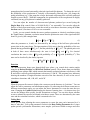
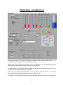
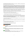
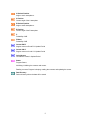
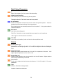
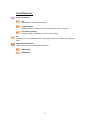
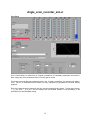
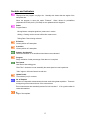
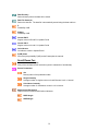
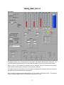
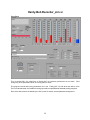
User’s Manual
Quantum Mechanics with Individual Photons
Simulations
M. Beck
Department of Physics, Whitman College, Walla Walla, WA 99362
[email protected] ; http://www.whitman.edu/~beckmk/QM/
These programs simulate experiments studying the behavior of photon pairs. The polarizations
of the two photons are correlated, and the correlations can be chosen to be either classical
(mixed states) or quantum mechanical (entangled states.) The programs are built from similar
programs used to control actual experiments, so they have the same look and feel as the
experimental programs. In particular, experimental noise is incorporated into the simulations in
a realistic way.
The Source
The experimental apparatus being simulated is shown in Fig. 1. A 405nm blue pump laser
(assumed to be vertically polarized) passes through a half-wave plate and a quartz plate. By
adjusting the rotation angle of the half-wave plate (using the 405nm wave plate angle control)
you can rotate the linear polarization of the
pump beam, which adjusts the relative
amplitudes of the horizontal and vertical
polarization components. [A note about wave
/2
plates: rotating a half-wave plate by an angle 
QP
rotates the polarization of the output beam by
2.] Tilting the quartz plate QP (using the
DC
Pump
Quartz plate angle control) adjusts the relative
laser
phase between the horizontal and vertical
polarizations.
Alice
The pump beam is then incident on the
downconversion crystals DC, which convert the
blue pump light into near-infrared photon pairs.
The two downconversion crystals are
sandwiched back-to-back, with their crystal axes
rotated at 90o with respect to each other. If the
downconverted photons are produced in the first
crystal, then a horizontally polarized pump
photon has become vertically polarized signal
and idler photons. If the downconversion occurs
in the second crystal, then a vertically polarized
1
Bob
/2
PBS
SPCM’s
/2
PBS
B
A
A'
B'
Fig 1 The experimental arrangement. Here /2
denotes a half-wave plate, QP denotes the quartz
plate, DC denotes the downconversion crystals,
PBS denotes a polarizing beam splitter, and SPCM
denotes the single photon counting modules.
pump photon has become horizontally polarized signal and idler photons. To change the ratio of
the probability of the production of vertically or horizontally polarized pairs, you change the
pump polarization (e.g., if the pump has a larger horizontal component, then vertically polarized
outputs are more likely). With this arrangement, the polarizations of the two photons are highly
correlated, but any given photon is randomly polarized.
You can adjust the number of downconverted photons produced per second (using the
Singles Rate (1/s) control.) Rates of 10,000-50,000 s-1 are reasonable. You can also adjust the
fraction of these downconversion events that result in coincidence detections (using the Coinc
fraction control.) Fractions of 0.05 or so are reasonable.
Lastly, you can control whether the source produces quantum or classical correlations (using
the Type: button.) Quantum correlation means that the polarization state of the signal and idler
beams is given by the entangled state
  a HH  bei VV ,
(1)
where the parameters a, b and  are determined by the settings of the half-wave plate and the
quartz plate in the pump beam. The interpretation of this state is that the probability of the two
photons having polarization HH is a2, and the probability of VV is b2. The photon pairs exist
in both of these states simultaneously: the state is both
correlations the state is either HH
HH
and VV . For classical
(with probability a2) or VV
(with probability b2.) This
state can be described by the density operator
ˆ  a 2 HH HH  b 2 VV VV .
(2)
Detection
The downconversion beams pass through half-wave plates; you control their rotation angles
using the A Desired Position and B Desired Position controls. These beams then pass through
polarizing beam splitters PBS which transmit horizontally polarized photons to detectors A and
B, and reflect vertically polarized photons to detectors A’ and B’. The programs have indicators
showing the numbers of singles detections on each of the four detectors, as well as four sets of
coincidence detections: AB, A’B, AB’, and A’B’.
Tweaking
When the program first starts it displays the count rates on the detectors in "real-time." You can
adjust the source parameters and measurement angles. By observing the different count rates at
different measurement angles you can adjust the source parameters to create the state that you
want. Changing the Update Period changes the detector counting time -- for shorter times you
can see the changes more quickly, but the fluctuations are larger. You can also choose whether
or not to subtract the expected accidental coincidence counts. These are determined by the count
rates and the coincidence window, which is assumed to be 8 ns.
Taking Data
When you are done adjusting the source parameters to create the state you're interested in, it’s
time to "take data." You set the parameters for this in the Data Taking Parameters box. Longer
update periods yield smaller fluctuations, more samples yield more reliable averages and error
2
estimates. The Run Speed button displays the magic of simulated experiments. If it is set to
Real Time then data taking proceeds at roughly the same pace as it would in a real experiment;
if it is set to 100x data taking proceeds at about 100 times faster than real experiments (wouldn't
it be nice if this worked with real experiments?)
Data will be saved in a folder inside the Data Directory path. The folder will be labeled by
the date, and the data file will be labeled by the date and time. The folders and data file will be
automatically created.
Once all the data taking parameters are set, press the Take Data button. Control will be
transferred to another program that automatically sets the measurement angles to the correct
values, writes the raw data to a file, and computes statistics of various quantities.
If you want to run the program again, go back to the original window and click the right
arrow in the upper left.
The Programs
More detailed help for each of the programs is given in the back of this manual.
Polarization_correlations_sim
This program allows you to observe the correlations between the polarizations of the two
downconverted photons. An interesting thing to explore is the difference between these
correlations for quantum and classical sources.
This program displays an indicator labeled P, which is the probability of obtaining an AB
coincidence. Thus, if the measurement wave plates are both set to 0, this is the probability that
the source produces photons in the state HH . If the measurement wave plates are both set to
22.5, this is the probability that the source produces photons in the state 45,  45 .
When you press the Take Data button for this program, the A wave plate remains fixed at
the angle set in the parameter A, while the B wave plate is scanned between 0° and 90°
(corresponding to polarization rotation of 0° to 180°).
A state with interesting polarization correlation is one of the four the Bell states:
 
1
 HH  VV
2
.
(3)
In order to create this state, we note that this state has equal probabilities for HH and VV .

Set the source for quantum correlations.

Set the A & B waveplates to 0°. Adjust the 405 waveplate angle so that the ratio of the
AB & A’B’ coincidences is roughly 1:1.
You may want to adjust the Update Period. If it is too short the counts will fluctuate a
lot, and it will be difficult to get a good reading. If it is too long you need to adjust things
very slowly, and wait for the screen to catch up. Values between 0.2 and 1.0 s should
work, depending on your count rates. You may also need to adjust the full scale reading
on your meters. You can do this by highlighting the value at the top of a scale, and typing
in a new value.
3

Now set the A & B waveplates to 22.5°. Adjust the Quartz plate angle to minimize the
A’B & AB’ coincidences.
Once the state is properly set, compare the quantum and classical correlations with the A wave
plate set to 0° and to 22.5°.
Hardy_Bell_sim
This program simulates two different tests of local realism: one originally due to John Bell [1],
and the other originally due to Lucian Hardy [2]. You can select which test is performed using
the Experimental Setup dial.
The Bell inequality is tested using the state of Eq. (3), and the source can be adjusted to
produce this state as described above. In this test one measures the quantity S, which is a
combination of four expectation values E. The values of E are obtained by measuring the
polarizations at 4 sets of angles (the expectation value for the current set of angles is displayed
by the E indicator.) The predictions of local realism are that S  2 , while for the state of Eq. (3)
the quantum prediction is S  2 2 , which clearly violates local realism. For more details about
the Bell test simulated here, see Refs. [3] and [4].
While running a Bell test, after pressing the Take Data button the program will calculate the
average and standard deviation of S. The program will also give a value called Violations, which
is the number of standard deviations by which S exceeds 2.
In the Hardy test one makes joint polarization measurements at four combinations of angles,
determined by two parameters,  and : P ,   , P , , P,    and P    , . You set
these angles in the program using the parameters Alpha and Beta (these parameters become
visible when the program is running, and Experimental Setup is set to Hardy.) The superscript
 refers to the perpendicular direction, e.g.      90 o . Given these 4 probabilities you can
compute the quantity

 

H  P ,   P ,    P    ,  P ,   .
(4)
As described in Ref. [5], if H < 0 the data is consistent with local realism, while if H > 0 local
realism is violated and we are forced to abandon some of our classical ideas.
The Hardy test can be performed using the state
 1  0.8 H
A
H
B
 0.2 V
A
V
B
.
(5)
With this state and the angles  and = 71°, the quantum mechanical prediction is that
P  ,    0.09 and all the other probabilities in Eq. (4) are nearly 0. This violates local realism.
Experimentally (and in the simulation program as well, because it includes realistic noise) one
cannot achieve 0 probabilities. With this in mind, a larger violation of the classical inequality
H  0 is achieved at slightly different values of  and  when using the state in Eq. (5) (see Ref.
[5] for more details.)
To create the state of Eq. (5), note that the probability of HH is 80%, and with both of the
wave plates set to 0° the P indicator and the P Meter read this probability.
4

Set the source for quantum correlations.

Make sure the Experimental Setup dial is set to Hardy, and that Update Period is set
to between 0.2 and 1.0s. Set the Subtract Accidentals? switch to Yes.

Make sure that Alpha is set to 55° and Beta is set to 71°.

Set the A & B waveplates to 0°. Adjust the 405 waveplate angle so that the ratio of the
AB & A’B’ coincidences is roughly 4:1. This is most easily done by watching the P
Meter, which reads the probability of an AB coincidence. You would like it to read 0.8.

Set your waveplates to measure P  ,   -- the half-wave plate settings needed to
achieve this measurement are shown in the section labeled H HWP Measurement
Angles. Adjust the Quartz plate angle to minimize this probability.

Check your state by setting the waveplates to measure P ,    and P    , . These
probabilities should be fairly small. Set your waveplate to measure P , ; this
probability should be larger than the others.
While running a Hardy test, after pressing the Take Data button the program will calculate
the average and standard deviation of the four probabilities and of H. The program will also give
a value called Violations, which is the number of standard deviations by which H exceeds 0.
References
[1] J. S. Bell, "On the Einstien-Podolsky-Rosen paradox," Physics 1, 195 (1964).
[2] L. Hardy, "Nonlocality for two particles without inequalities for almost all entangled states,"
Phys. Rev. Lett. 71, 1665 (1993).
[3] D. Dehlinger and M. W. Mitchell, "Entangled photon apparatus for the undergraduate
laboratory," Am. J. Phys. 70, 898 (2002).
[4] D. Dehlinger and M. W. Mitchell, "Entangled photons, nonlocality, and Bell inequalities in
the undergraduate laboratory," Am. J. Phys. 70, 903 (2002).
[5] J. A. Carlson, M. D. Olmstead, and M. Beck, "Quantum mysteries tested: An experiment
implementing Hardy's test of local realism," Am. J. Phys. 74, 180 (2006).
5
6
Polarization_correlations.vi
Front Panel
This program allows you to examine the polarization correlations between downconversion beams. You
can select either entangled (quantum) or mixed (classical) states.
Help for each of the controls and indicators can be obtained from the Contextual Help window
(Help>>Show Context Help) by mousing over each control or indicator.
This program does not record data to a file right away, but displays the counters in real time so that you
can adjust the source and measurement parameters.
Once everything is aligned and the parameters are set, you press the "Take Data" button. This transfers
control to another program which records a data set and saves it to a file.
You create the source state that you want by adjusting the parameters in the "Source" box. Adjusting the
7
"405 waveplate angle" adjusts the ratio of |HH> to |VV> photons. Adjusting the "Quartz plate angle"
adjusts the relative phase between these two terms.
After initialization the program simply loops and displays the counts in a given time window (determined
by the "update Period" control in the upper left.) Status reads "Reading Counters". This is useful for
tweaking the source and measurement parameters. Waveplates in front of the analyzing polarization
beamsplitters are moved by setting the desired waveplate angles in the " A(B) Desired Position" controls.
Remember that these are WAVEPLATE angles; since polarization rotates twice as fast as the waveplate,
the corresponding polarization angles are twice as large. For example, if the A waveplate angle is set to
22.5 deg, the polarization measured on the A detector is 45 deg, while the A' detector measures -45deg.
Nothing is written to disk until the parameters are chosen and the "Take Data" button is pressed. This
loads a second VI that records and saves data to disk-it is placed in a folder labeled by date within the
folder specified in "Data Directory". This folder will be created if it doesn't already exist.
Parameters for this data acquisition phase are set in the "Data Taking Parameters" box. During data
acquisition the program will set the waveplate angles as follows:
The waveplate for the A beam is fixed by the Data Taking Parameter "A".
The angle of waveplate B is scanned over 17 equally spaced values: 0, 5.625, 11.25, ...
Again, remember that these are WAVEPLATE angles, and since polarization rotates twice as fast as the
waveplate, the corresponding polarization angles are twice as large. So, the A polarization angle is twice
what is set by the A control, while the B polarization angles are 0, 11.25, 22.5, ... What gets recorded in
the data file are waveplate angles, NOT polarization angles.
You can change the scales of the bar-graph indicators by highlighting the number at the top of the scale
and typing in a new maximum value.
Note that scrolling the window down displays the wavefunction and density matrix of the polarization
state.
The coincidence windows are assumed to have a coincidence resolution time of 8 ns. This is used for
computing and subtracting accidental coincidences.
To re-run the program, click the right-arrow at the top left.
Controls and Indicators
Update Period
Time window (in S) for the counters during setup phase (i.e., before the "Take Data"
button is pressed.) Readings update once each time window if "Status" reads "Reading
Counters".
Stop
Use this to stop. It takes a little longer, but this way, the board gets reset. If you stop
some other way you'll probably need to quit Labview and restart; you may even need to
reboot the computer.
Subtract Accidentals?
Determines whether or not accidental coincidences are subtracted. Controls data taking
mode as well as tweaking mode. Assumes a coincidence window of 8 ns.
8
A Desired Position
Angle to set A waveplate to.
A Position
Current angle of the A waveplate.
B Desired Position
Angle to set B waveplate to.
B Position
Current angle of the B waveplate.
P
Probability of AB.
P Meter
Probability of AB
Counts B & B'
Singles counts on B and B' in Update Period
Counts A & A'
Singles counts on A and A' in Update Period
Coincidences
Coincidence counts in Update Period
Status
Program Status
Initializing: initializing the counters and motors.
Reading counters: Program is looping, reading the counters and updating the screen.
Data Directory
Path to directory where the data will be saved.
9
Data Taking Parameters
A
Angle of A waveplate--fixed for duration of the data taking.
Update Period (Data Run)
Time window (in S) for counters during data acquisition.
This applies after the "Take Data" button has been pressed.
No. of Samples
Number of independent measurements that are made during data acquisition. These are
averaged to get the mean and error of the measurement.
Error measurements are essentially useless if this is less than 5. 10 is a good number for
reasonable statistics.
Run Speed:
How fast the data taking goes:
"Real Time": simulation runs at essentially the same speed as a real experiment
"100x": apporx. 100 times faster than real time.
Take Data
Leave the setup "tweaking" mode and switch to data acquisition mode.
Source
405 waveplate angle
Corresponds to adjusting the angle of the 405nm half-wave plate to change the
polarization of the blue pump beam. The numbers correspond to the actual waveplate
angle.
Quartz plate angle
Adjusts the relative phase between the |HH> and |VV> components of the state. A full
range of phase adjustments is from -180 to +180.
Singles Rate (1/s)
Average singles detection rates (per second) in the A and B beams. Higher numbers
mean more photodetections per second.
Coinc faction
Fraction of the singles rate that becomes coincidences. 0.10 (10%) is high. 0.05 is more
reasonable.
Type:
Quantum: Polarization entangled state.
Classical: Polarization mixed state.
10
Scroll Down For:
Source Parameters
rho
Density matrix of the polarization state.
Singles Intensity
Average number of singles counts on A and B beams in a 0.1s interval.
Coincidence Intenstiy
Average number of coincidence counts in a 0.1s interval.
Psi
Wavefunction of the polarization state. Only defined (and hence visible) for a quantum
state.
Measurement Parameters
Copies of the A Position and B Position indicators
HWP1 Angle
HWP2 Angle
11
Angle_scan_recorder_sim.vi
Front Panel
This VI should ONLY be called from an "Angular_correlations" VI--necessary parameters are set there.
Don't change any of the parameters while it's running-just let it finish.
This program records data (using parameters set in the "Angular_correlations" VI) and saves the data to
a file. The file is tab-delimited, and suitable for being imported into spreadsheets and data plotting
programs.
Each of the data columns is labeled by the time, and the parameter being saved. The last two columns,
"...._P_ave" and "..._P_st_dev", are the average and the standard deviation of the probability of AB
coincidences for that waveplate setting.
12
Controls and Indicators
Operation
Displays what the program is trying to do. Normally this shows what the angles of the
waveplates are.
When the program is done this reads "Finished." When Values for probabilities
(expectations for Bell) and H (S for Bell) are not updated until this happens.
Status
Program Status:
Moving Motors: waveplate (polarizer) motors are in motion.
Waiting: Clearing out the counter buffers after motors move.
Taking Data: Data is being collected.
B Position
Current position of B waveplate
A position
Current position of A waveplate
Subtract Accidentals?
Determines whether or not accidental coincidences are subtracted.
Progress
Rough indication of what percentage of the data run is complete.
Run Speed:
How fast the data taking goes:
"Real Time": simulation runs at essentially the same speed as a real experiment
"100x": approx. 100 times faster than real time.
Update Period
Time window (in s) for counters.
No. of Samples
Number of independent measurements that are made during data acquisition. These are
averaged to get the mean and error of the measurement.
Error measurements are essentially useless if this is less than 5. 10 is a good number for
reasonable statistics.
A
Angle of A waveplate.
13
Data Directory
Path to directory where the data will be saved.
Data File Saved As:
Path to the data file. The data file is automatically named using the date and time.
P
Probability of AB.
P Meter
Probability of AB
Counts B & B'
Singles counts on B and B' in Update Period
Counts A & A'
Singles counts on A and A' in Update Period
Coincidences
Coincidence counts in Update Period
P(A,B) Chart
Plot of the joint probability P(A,B) as the B waveplate is scanned.
Scroll Down For:
coincidence resolution (ns)
Array of the coincidence time resolutions (used in subtraction of accidentals).
Source Parameters
rho
Density matrix of the polarization state.
Singles Intensity
Average number of singles counts on A and B beams in a 0.1s interval.
Coincidence Intenstiy
Average number of coincidence counts in a 0.1s interval.
Measurement Parameters
Copies of the A Position and B Position indicators
HWP1 Angle
HWP2 Angle
14
Hardy_Bell_sim.vi
Front Panel
This program allows you to simulate tests of local realism, using both a Bell-test and a Hardy-test. You
can select either entangled (quantum) or mixed (classical) states to see how they influence the results.
Help for each of the controls and indicators can be obtained from the Contextual Help window
(Help>>Show Context Help) by mousing over each control or indicator.
This program does not record data to a file right away, but displays the counters in real time so that you
can adjust the source and measurement parameters.
Once everything is aligned and the parameters are set, you press the "Take Data" button. This transfers
control to another program which records a data set and saves it to a file.
15
You create the source state that you want by adjusting the parameters in the "Source" box. Adjusting the
"405 waveplate angle" adjusts the ratio of |HH> to |VV> photons. Adjusting the "Quartz plate angle"
adjusts the relative phase between these two terms.
After initialization the program simply loops and displays the counts in a given time window (determined
by the "update Period" control in the upper left.) Status reads "Reading Counters". This is useful for
tweaking the source and measurement parameters. Waveplates in front of the analyzing polarization
beamsplitters are moved by setting the desired waveplate angles in the " A(B) Desired Position" controls.
Remember that these are WAVEPLATE angles; since polarization rotates twice as fast as the waveplate,
the corresponding polarization angles are twice as large. For example, if the A waveplate angle is set to
22.5 deg, the polarization measured on the A detector is 45 deg, while the A' detector measures -45deg.
Nothing is written to disk until the parameters are chosen and the "Take Data" button is pressed. This
loads a second VI that records and saves data to disk-it is placed in a folder labeled by date within the
folder specified in "Data Directory". This folder will be created if it doesn't already exist.
Parameters for this data acquisition phase are set in the "Data Taking Parameters" box. During data
acquisition the program will set the waveplate angles to those shown in the box labeled "HWP
Measurement Angles". Angles for a Bell measurement are fixed. Angles for a Hardy measurement are
determined from the controls "Alpha" and "Beta".
At the end of data taking the program will tell you (and write to the file) an average value of S (for Bell), or
H (for Hardy), as well as standard deviations for these quantities. It also gives you a number for
"Violations," which is a number of standard deviations that the value of S or H violates local realism.
Positive values for violations are consistent with quantum mechanics but not local realism, while negative
values are consistent with classical mechanics and local realism.
You can change the scales of the bar-graph indicators by highlighting the number at the top of the scale
and typing in a new maximum value.
Note that scrolling the window down displays the wavefunction and density matrix of the state.
The coincidence windows are assumed to have a coincidence resolution time of 8 ns. This is used for
computing and subtracting expected accidental coincidences.
Controls and Indicators
Update Period
Time window (in S) for the counters during setup phase (i.e., before the "Take Data"
button is pressed.) Readings update once each time window if "Status" reads "Reading
Counters".
Stop
Use this to stop. It takes a little longer, but this way, the board gets reset. If you stop
some other way you'll probably need to quit Labview and restart; you may even need to
reboot the computer.
Experimental Setup
Which Measurement to perform.
Hardy: Hardy measurement (4 detectors)
S: Bell measurement (4 detectors)
16
Subtract Accidentals?
Determines whether or not accidental coincidences are subtracted. Controls data taking
mode as well as tweaking mode. Assumes a coincidence window of 8 ns.
A Desired Position
Angle to set A waveplate to.
A Position
Current angle of the A waveplate.
B Desired Position
Angle to set B waveplate to.
B Position
Current angle of the B waveplate.
Counts B & B'
Singles counts on B and B' in Update Period
Counts A & A'
Singles counts on A and A' in Update Period
Coincidences
Coincidence counts in Update Period
P (Hardy Measurements)
Probability of AB.
P Meter (Hardy Measurements)
Probability of AB
E (Bell Measurements)
Expectation Value
E Meter (Bell Measurements)
Expectation Value
Alpha (Hardy Measurements)
Angle Alpha used in the Hardy measurement.
Beta (Hardy Measurements)
Angle Beta used in the Hardy measurement.
H HWP Measurement Angles (Hardy Measurements)
HWP angles at which probabilities that determine H will be measured. Determined from
Alpha and Beta settings.
Useful so that you know which angles to set waveplate to when tweaking.
S HWP Measurement Angles (Bell Measurements)
HWP angles at which expectation values that determine S will be measured.
Useful so that you know which angles to set waveplates to when tweaking. Angles
labeled + correspond to expectations you want to be as positive as possible, while those
labeled - should be as negative as possible.
17
Status
Program Status
Initializing: initializing the counters and motors.
Reading counters: Program is looping, reading the counters and updating the screen.
Data Taking Parameters
Update Period (Data Run)
Time window (in S) for counters during data acquisition.
This applies after the "Take Data" button has been pressed.
No. of Samples
Number of independent measurements that are made during data acquisition. These are
averaged to get the mean and error of the measurement.
Error measurements are essentially useless if this is less than 5. 10 is a good number for
reasonable statistics.
Run Speed:
How fast the data taking goes:
"Real Time": simulation runs at essentially the same speed as a real experiment
"100x": apporx. 100 times faster than real time.
Take Data
Leave the setup "tweaking" mode and switch to data acquisition mode.
18
Source
405 waveplate angle
Corresponds to adjusting the angle of the 405nm half-wave plate to change the
polarization of the blue pump beam. The numbers correspond to the actual waveplate
angle.
Quartz plate angle
Adjusts the relative phase between the |HH> and |VV> components of the state. A full
range of phase adjustments is from -180 to +180.
Singles Rate (1/s)
Average singles detection rates (per second) in the A and B beams. Higher numbers
mean more photodetections per second.
Coinc faction
Fraction of the singles rate that becomes coincidences. 0.10 (10%) is high. 0.05 is more
reasonable.
Type:
Quantum: Polarization entangled state.
Classical: Polarization mixed state.
Scroll Down For:
Source Parameters
rho
Density matrix of the polarization state.
Singles Intensity
Average number of singles counts on A and B beams in a 0.1s interval.
Coincidence Intenstiy
Average number of coincidence counts in a 0.1s interval.
Psi
Wavefunction of the polarization state. Only defined (and hence visible) for a quantum
state.
Measurement Parameters
Copies of the A Position and B Position indicators
HWP1 Angle
HWP2 Angle
19
Hardy-Bell-Recorder_sim.vi
Front Panel
This VI should ONLY be called from a "Hardy_Bell" VI--necessary parameters are set there. Don't
change any of the parameters while it's running-just let it finish.
This program records data (using parameters set in the "Hardy_Bell" VI) and saves the data to a file.
The file is tab-delimited, and suitable for being imported into spreadsheets and data plotting programs.
Each of the data columns is labeled by the time (in the file name), and the parameter being saved.
20
Controls and Indicators
Operation
Displays what the program is trying to do. Normally this shows what the angles of the
waveplates are.
When the program is done this reads "Finished." When Values for probabilities
(expectations for Bell) and H (S for Bell) are not updated until this happens.
Status
Program Status:
Moving Motors: waveplate (polarizer) motors are in motion.
Waiting: Clearing out the counter buffers after motors move.
Taking Data: Data is being collected.
B Position
Current position of B waveplate
A position
Current position of A waveplate
Subtract Accidentals?
Determines whether or not accidental coincidences are subtracted.
Progress
Rough indication of what percentage of the data run is complete.
Update Period
Time window (in s) for counters.
No. of Samples
Number of independent measurements that are made during data acquisition. These are
averaged to get the mean and error of the measurement.
Error measurements are essentially useless if this is less than 5. 10 is a good number for
reasonable statistics.
Alpha
Angle Alpha used in the Hardy measurement.
Beta
Angle Beta used in the Hardy measurement.
21
Data Directory
Path to directory where the data will be saved.
Data File Saved As:
Path to the data file. The data file is automatically named using the date and time.
P (Hardy Measurements)
Probability of AB.
E (Bell Measurements)
Expectation Value
Counts B & B'
Singles counts on B and B' in Update Period
Counts A & A'
Singles counts on A and A' in Update Period
Coincidences
Coincidence counts in Update Period
Results
S (Bell measurement only)
Mean Value of S. Updated when "Operation" reads "Finished".
Stdev(S) (Bell measurement only)
Standard deviation of S. Updated when "Operation" reads "Finished".
Violations(S) (Bell measurement only)
Number of standard deviations that S is above 2. Updated when "Operation" reads
"Finished".
H (Hardy measurement only)
Mean value of H. Updated when "operation" reads "Finished".
Stdev(H) (Hardy measurement only)
Standard Deviation of H. Updated when "operation" reads "Finished".
Violations(H) (Hardy measurement only)
Number of standard deviations that H is above 1.
"Finished".
Updated when "operation" reads
P
Stdev(P)
Average and standard deviation of the 4 probabilities that make up H.
22
Scroll Down For:
Run Speed:
How fast the data taking goes:
"Real Time": simulation runs at essentially the same speed as a real experiment
"100x": approx. 100 times faster than real time.
coincidence resolution (ns)
Array of the coincidence time resolutions (used in subtraction of accidentals).
Source Parameters
rho
Density matrix of the polarization state.
Singles Intensity
Average number of singles counts on A and B beams in a 0.1s interval.
Coincidence Intenstiy
Average number of coincidence counts in a 0.1s interval.
Measurement Parameters
Copies of the A Position and B Position indicators
HWP1 Angle
HWP2 Angle
23