Download Resolution Improvement of Digitized Images

University of West Bohemia in Pilsen
Faculty of Applied Sciences
Department of Computer Science and Engineering
Diploma Thesis
Resolution improvement of digitized
images
Plzeň, 2004
Libor Váša
Abstract
This work focuses on possibilities of enhancing resolution of digitized images gained by
CCD elements. Image pre-processing is described, including algorithms for demosaicking,
colour balancing and colour scaling. Resolution enhancement techniques are described,
mentioning interpolations and focussing on techniques working with multiple images of
unchanged scene.
Frequency domain and space domain approaches are described and an improved algorithm
is proposed, exploiting knowledge about the real CCD elements. Implementation of image
enhancement techniques is described and results of experiments with both simulated and real
images are presented.
1
Table of contents
Abstract.................................................................................................................................. 1
Acknowledgements ............................................................................................................... 5
1. Introduction .................................................................................................................... 6
2. CCD sensors................................................................................................................... 7
2.1
Basic kinds of CCD sensors ................................................................................... 7
2.1.1
Rectangular CCD sensors using Bayer array ................................................. 7
2.1.2
Multilayer rectangular CCD sensor................................................................ 8
2.1.3
Octagonal CCD elements ............................................................................... 8
2.2
Image data processing ............................................................................................ 9
2.2.1
Demosaicking................................................................................................. 9
2.2.2
White Balancing........................................................................................... 14
2.2.3
Colour scaling .............................................................................................. 15
2.3
Influence of pre-processing on SR algorithms ..................................................... 17
3. Resolution enhancement .............................................................................................. 18
3.1
Super Resolution problem specification .............................................................. 18
3.2
Frequency domain methods ................................................................................. 19
3.2.1
Registration methods used for frequency domain methods ......................... 20
3.2.2
Properties of frequency domain approach relevant to CCD sourced images21
3.3
Space domain methods......................................................................................... 21
3.3.1
Unifying notation for space domain SR ....................................................... 21
3.3.2
Iterative Backprojection ............................................................................... 22
3.3.3
Zomet robust method ................................................................................... 23
3.3.4
Farsiu robust method.................................................................................... 24
3.3.5
Smoothness assumption ............................................................................... 24
3.3.6
Registration methods used for space domain SR ......................................... 25
3.3.7
Properties of space domain approach relevant to CCD sourced images...... 26
3.4
Improved algorithm derivation............................................................................. 26
4. Implementation............................................................................................................. 28
4.1
Data structures...................................................................................................... 28
4.2
Simulated images ................................................................................................. 29
4.3
Noise simulation................................................................................................... 30
4.4
Registration .......................................................................................................... 30
4.5
Smoothness prior implementation........................................................................ 31
4.6
Implemented smoothing filters............................................................................. 32
4.6.1
Farsiu smoothing .......................................................................................... 32
4.6.2
Weighted neighbourhood averaging filter.................................................... 32
4.6.3
Edge preserving smoothing filter ................................................................. 33
4.7
Implemented SR methods .................................................................................... 33
4.7.1
Iterated Backprojection ................................................................................ 34
4.7.2
Zomet robust method ................................................................................... 36
4.7.3
Farsiu robust method.................................................................................... 36
4.8
RAW data loading................................................................................................ 37
4.9
Image data loading ............................................................................................... 38
4.10 Batch processing methods.................................................................................... 39
4.10.1 Super-resolution of RGB images ................................................................. 39
4.10.2 Batch experiments ........................................................................................ 41
5. Experiments with simulated data ................................................................................. 42
2
5.1
Accuracy testing................................................................................................... 42
5.2
Robustness testing ................................................................................................ 47
5.3
Speed tests ............................................................................................................ 49
5.4
Smoothness tests .................................................................................................. 50
5.5
Influence of demosaicking on the SR process ..................................................... 51
5.6
SR results compared to single image resolution enhancement ............................ 53
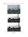
6. Experiments with real data........................................................................................... 54
6.1
Images taken from camera held in hand............................................................... 54
6.2
Images taken from lying camera .......................................................................... 55
6.3
Images taken from tripod ..................................................................................... 56
7. Future work .................................................................................................................. 57
8. Conclusion.................................................................................................................... 58
Used abbreviations .............................................................................................................. 58
References ........................................................................................................................... 59
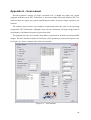
Appendix A – User manual ................................................................................................. 60
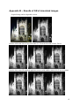
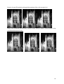
Appendix B – Results of SR of simulated images .............................................................. 63
Appendix C – MRW format description ............................................................................. 66
3
I hereby declare that this diploma thesis is completely my own work and that I used only
the cited sources.
Pilsen, 21.5.2004
Libor Váša
4
Acknowledgements
The author would like to thank to Mr. Tom Crick, who kindly checked a large part of this
work for language mistakes.
This work was supported by Microsoft Research – project No. 2003-178
5
1. Introduction
The fast development of computer technologies has become a standard during the last few
decades. This state is usually represented by improvements in quantitative parameters of
computer hardware, but also major qualitative changes can be observed in some areas of
development. These breakthroughs are usually connected with considerable drops in prices,
which allows for wider markets producing larger profits, which can be reinvested into
research aimed to further reduction of manufacturing costs.
A good example of such developments are changes on the market of still cameras, where
digital equipment recently gained position comparable to traditional analog cameras.
Consumer digital cameras provide sufficient quality for amateur shooting and the advantage
of digital processing of images attracts many buyers. However, professional users still see
considerable disadvantages of digital photography, represented by smaller dynamic range of
images and low resolution, which limits the use of digital images to small format prints. In
this work we would like to show methods of improving resolution of digital imagery without
using a CCD (Charge Coupled Device) element with higher resolution. One way of achieving
such goal is to combine multiple shifted low resolution images into one with higher
resolution. Such a process is usually denoted as Super Resolution (SR).
First of all we will need to find out what kind of data can be obtained from an ordinary
digital camera, what algorithms are used to process such data and how does such processing
affect eventual resolution enhancement. Subsequently we will explore existing Super
Resolution techniques, considering their properties relevant to consumer level digital cameras.
We will choose some of the methods for reference implementation and we will derive a
modified method that will consider specific properties of current CCD sensors. We will
compare results of such method to reference methods results and state conclusions about the
improvement gained.
We will derive algorithms as general as possible, and we will verify our results
experimentally. Our testing hardware will be a digital camera that employs common
technologies (such as RGB Bayer array CCD) and provides RAW data file, allowing us to
alter most of image pre-processing.
6
2. CCD sensors
2.1 Basic kinds of CCD sensors
With reference to our goals we will split the CCD elements used in current consumer level
cameras according to the shape of the sensor cell and to the method used to gain RGB
samples at each pixel location.
Two basic shapes of cell are currently used: octagonal (SuperCCD by FujiFilm) and more
common rectangular, that in most cases uses square cells. Samples of RGB at each pixel
location are either measured at each pixel location (multilayer Foveon CCD by Sigma) or
computed using special kind of interpolation denoted as demosaicking.
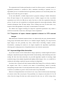
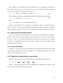
2.1.1 Rectangular CCD sensors using Bayer array
A Rectangular CCD sensor with one layer of light-sensitive cells is used in most current
digital cameras. Each cell is covered by a colour filter that only lets through certain
wavelengths. Usually three types of filters are used, allowing the red, green or blue part of the
spectrum, and the values gained are interpreted as the R, G or B components of the resulting
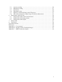
pixel. The most commonly used layout of RGB filters is denoted as the Bayer array, which is
shown in figure 2.1. Equal amounts of red and blue samples are gained, while green is
sampled at double frequency due to the human eye is most sensitive to green colours.
It is also possible to use different wavelengths, as Nikon, for example, uses C-Y-G-M
(Cyan, Yellow, Green and Magenta) filter array for its Coolpix digital camera series, while
Sony uses R-G-B-E (Red, Green, Blue and Emerald) for its DSC-F828 model. These
modifications usually aim to enlarge the colour gamut of the device and therefore improve the
colour response of the camera. Non-Bayer CCDs require different demosaicking algorithms,
but their properties are generally equal to the Bayer array CCDs.
It is important to realise that in any of these cases only one component of usual three- or
four- component colour representation is measured at each pixel location. The remaining two
or three values need to be computed artificially, employing interpolation techniques. This
process and its effects will be described later.
7
R
G
R
G
R
G
R
G
G
B
G
B
G
B
G
B
R
G
R
G
R
G
R
G
G
B
G
B
G
B
G
B
R
G
R
G
R
G
R
G
G
B
G
B
G
B
G
B
Figure 2.1 – Bayer colour array
2.1.2 Multilayer rectangular CCD sensor
Only one manufacturer currently provides digital cameras for the consumer market that
employs a CCD element capable of measuring all RGB values at each pixel location. Sigma
Foveon technology uses three layers of light-sensitive elements, each measuring a particular
range of wavelengths and letting the rest of the spectra through.
In such case no demosaicking is required, as all the information is measured directly,
which allows for faster processing and better images without a possibility of interpolation
artifacts. The main downside to this approach is the current high production cost of Foveon
CCD elements, which makes any camera using such technology many times more expensive
than Bayer array based camera with equal resolution (Sigma states a 10 MegaPixel sensor, but
this number relates to number of light-sensitive cells, actual resolution of taken picture is only
3.3MPx).
2.1.3 Octagonal CCD elements
Cameras produced by Fujifilm use an octagonal shape of light-sensitive elements, which
allows for smaller inter-pixel distance and therefore produces more accurate images. Sensors
that use this approach are denoted as SuperCCD, currently fourth generation is available.
For the purposes of this work SuperCCD is unfit, as it is (in comparison to rectangular
CCDs) much harder to simulate a degradation process represented by them. Moreover, the
latest generation of SuperCCD introduces separation of the light-sensitive cells into two parts
with different saturation properties, which allows for a wider dynamic range of the camera,
but makes it practically impossible to simulate the process of image capturing without a very
precise knowledge of sizes, shapes and positions of light-sensitive cells. Such knowledge is
currently not available, as it is commercially sensitive, and even with such knowledge the
simulation would be very complicated.
8
2.2 Image data processing
In following part we will consider a rectangular CCD element employing a RGB Bayer
array. Most of the processing methods are used in multilayer CCDs as well, with the only
difference being skipping the demosaicking step.
In this context, data processing includes all operations performed on digital data obtained
from the CCD in order to get a standard computer image, i.e. a TIFF or JPEG file. All of these
operations are usually performed by fast dedicated hardware contained within the camera.
Alternatively these operations can be performed by specialised software working with RAW
data file gained from the camera.
Generally the processing consists of three or four separate steps. At first, all RGB values
are reconstructed at each pixel position (demosaicking). Subsequently the image undergoes a
procedure which adjusts the colour temperatures of the image (white-balancing), followed by
transferring the image into logarithmic space (scaling). Resulting values may be compressed
to an image format (JPEG, TIFF).
2.2.1 Demosaicking
As mentioned before, demosaicking is a process transforming incomplete RGB data from a
CCD into a matrix containing RGB triple at each pixel location. Multiple algorithms were
proposed to achieve this goal, because simple interpolation leads to visible artefacts.
Algorithms used in real digital cameras are usually modifications of some of the
algorithms presented here. According to experiments, many algorithms used by camera
hardware and RAW data software differ from each other and their exact specification is
usually not publicly available.
2.2.1.1 Decreasing resolution
One intuitive approach to demosaicking may be decreasing the resolution of the image
gained by the CCD to one half of the original value. The new pixel in this “subsampled”
image now contains one value for red channel, one value for blue channel and two values for
green channel. We can consider these values to be RGB values of the low resolution grid
pixel.
Such an approach has two main drawbacks. An obvious one is that we have degraded the
image quality by reducing its resolution considerably. The less obvious, but equally
important, is a problem denoted as colour fringing.
9
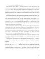
If there is, for example, a unit step in intensity of light in the original image, we would get
a situation as illustrated by fig. 2.2. For the first two rows we will get the following values:
100%
100%
100%
100%
100%
50%
50%
0%
0%
0%
0%
0%
Combining these values, we will get three pixels. The first pixel will be full white
(RGB 1:1:1), the second will be orange (RGB 1:0.5:0) and the last will be full black.
For the pixel on the edge of the step, we not only get invalid lightness, but also invalid hue.
This results in coloured stripes along the intensity edges that are very disconcerting for human
perception. The problem of colour fringing is common for some of the following methods and
more sophisticated methods aim to reduce its negative effects.
R
G
R
G
R
G
G
B
G
B
G
B
R
G
R
G
R
G
G
B
G
B
G
B
R
G
R
G
R
G
G
B
G
B
G
B
Figure 2.2 – unit step measured by Bayer colour array
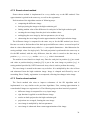
2.2.1.2 Linear interpolation
Another intuitive approach to demosaicking is to use simple linear interpolation, setting a
value of the unknown component equal to the mean of values measured in the local (usually
unit width) neighbourhood of the pixel.
This method gives good results for interpolation of the G component, where 4 samples in
the closest neighbourhood are always available. For the remaining channels, R and B, two
cases can be distinguished. For one third of cases four values are measured in the closest
neighbourhood, being diagonally adjacent to the computed value. In the remaining two thirds
of cases, only two adjacent measured values are available, making the mean less reliable.
Linear interpolation solves the problem of degrading the image’s resolution, but problems
with colour fringing exists even here, as illustrated in fig. 2.3 for single line of Bayer array.
10
original colour
Bayer array
measured values
interpolated complementary values
final pixel colour
100% 100% 100%
0%
100% 100% 50% 50%
0%
0%
0%
0%
Figure 2.3 – colour fringing caused by linear interpolation
2.2.1.3 Constant hue based interpolation
This method (proposed in [Cok87]) tries to reduce colour fringing by keeping constant hue
in the interpolation neighbourhood. In this algorithm, hue is defined as R/G and B/G ratios,
where R and B are treated as chrominance values and G is considered to be luminance value.
The first step of the algorithm populates all pixel locations with G value using linear
interpolation. In the second step, defined hue is linearly interpolated from surrounding points
and used with G value to produce the chrominance values. Let us now consider the Bayer
array shown in figure 2.4.
R11
G12
R13
G14
R15
G16
G21
B22
G23
B24
G25
B26
R31
G32
R33
G34
R35
G36
G41
B42
G43
B44
G45
B46
R51
G52
R53
G54
R55
G56
G61
B62
G63
B64
G65
B66
Figure 2.4 – part of Bayer colour array
Computation may then be expressed as follows:
R22 = G22
R11 R13 R31 R33
+
+
+
G11 G13 G31 G33
4
(2.1)
for the case of four diagonal neighbours, or as
R31 R33
+
G31 R33
R32 = G32
2
(2.2)
for the case of two neighbours.
As one can see, the problem remains of including only two adjacent measured values for
two thirds of chrominance computations.
11
2.2.1.4 Median filtered interpolation (Freeman demosaicking)
This method (proposed in [Free88]) also attempts to reduce the effects of fringing by
removing sudden steps in hue, interpreted in a similar way as in the previous algorithm.
Median filtering is used to remove such jumps while preserving important hue changes.
In the first step of the algorithm, complete linear interpolation of RGB components is
performed. Difference images R-G and B-G are subsequently constructed and filtered by 3x3
or 5x5 median filter. Resulting differences are then used with original measurements to
compute all the RGB values in each pixel. This is possible as we have one value and two
differences for each pixel.
Unit steps are correctly reconstructed when the 5x5 median is used, while the 3x3 median
does not help. Unfortunately, the 5x5 median may remove some important details from the
image, degrading its sharpness.
2.2.1.5 Larroche – Prescott algorithm
This method (proposed in [Laro94]) exploits a simple idea, that when a sharp edge runs
through a pixel it is more accurate to interpolate missing value from values measured in the
direction of the edge rather than from values measured across the edge. At each pixel a
classifier value is computed, which will detect the direction of a possible edge. According to
this value an estimator is chosen. The algorithm works in a two step fashion, in the first step
values of G at each pixel location are computed using following classifiers:
a = abs[(B42 + B46 ) / 2 − B44 ]
(2.3)
b = abs[(B24 + B64 ) / 2 − B44 ]
Note that classifiers are closely related to first order partial derivatives and therefore
express amount of change in vertical and horizontal direction. Subsequently, following
estimators are used according to values of classifiers:
G44 = (G43 + G45 ) / 2
where a < b
G44 = (G34 + G54 ) / 2
where a > b
G44 = (G43 + G45 + G34 + G54 ) / 4
where a = b
(2.4)
Following chrominance computation employs idea of constant hue proposed previously.
2.2.1.6 Hamilton – Adams algorithm
The algorithm proposed in [Ham97] uses the same idea as in the previous algorithm, only
includes second order partial derivative related classifiers and estimators to guess the
12
direction of the edge more precisely. The algorithm again works in a two-step fashion, first
interpolating green component using following classifiers:
a = abs (− A3 + 2 A5 − A7 ) + abs (G4 − G6 )
(2.5)
b = abs (− A1 + 2 A5 − A9 ) + abs (G2 − G8 )
Indexing of formulas presented relate to cross neighbourhood illustrated in fig. 2.5, value A
represents measured chrominance value (either R or B). According to values of these
classifiers one of following G estimators is chosen:
G5 = (G4 + G6 ) / 2 + (− A3 + 2 A5 − A7 ) / 2
where a < b
G5 = (G2 + G8 ) / 2 + (− A1 + 2 A5 − A9 ) / 2
where b < a
(2.6)
G5 = (G2 + G4 + G6 + G8 ) / 4 + (− A3 − A1 + 4 A5 − A7 − A9 ) / 4 where a = b
For some chrominance values estimation is instead of constant hue computation used
similar classifier/estimator scheme. For the two neighbours case is used following estimator
without any condition:
A2 = ( A1 + A3 ) / 2 + (−G1 + 2G2 − G3 ) / 2
(2.7)
A4 = ( A1 + A7 ) / 2 + (−G1 + 2G4 − G7 ) / 2
For the diagonal neighbours is following classifier used to decide the direction of the edge:
a = abs (−G3 + 2G5 − G7 ) + abs ( A3 − A7 )
(2.8)
b = abs (−G1 + 2G5 − G9 ) + abs ( A1 − A9 )
Value indexing used in these formulas relate to unit neighbourhood illustrated in fig. 2.6.
Subsequently, one of following estimators is chosen:
A5 = ( A3 + A7 ) / 2 + (−G3 + 2G5 − G7 ) / 2
where a < b
A5 = ( A1 + A9 ) / 2 + (−G1 + 2G5 − G9 ) / 2
where a > b
A5 = ( A1 + A3 + A7 + A9 ) / 2 + (−G1 − G3 + 4G5 − G7 − G9 ) / 4
(2.9)
where a = b
Please note that in this and in the previous algorithm, not only values of the estimated
components are considered in the estimation process. This implies that demosaicking results
of these methods differ when separate channels are used (values of R and B influence
estimates of G and vice versa).
A3
G4
A1
G2
A5
G8
A9
G6
A7
Figure 2.5 – neighbourhood used for G classifiers in Hamilton – Adams algorithm
13
A1
G4
A7
G2
C5
G8
A3
G6
A9
Figure 2.6 – neighbourhood used for chrominance classifiers in Hamilton – Adams
algorithm
2.2.1.7 Loopy propagation demosaicking
In some recent work [Grant] an idea of employing loopy belief propagation networks
framework is used for demosaicking. This approach is mainly used for the estimation of
chrominance channels, but has no positive effect on the better sampled luminance values. The
algorithm treats colour values as “beliefs” of cells that are iteratively updated using message
passing algorithm between neighbouring cells. The number of iterations must be artificially
limited because after a certain number of iterations the mean error starts to rise, as irrelevant
information from too distant cells starts to influence the beliefs.
In this algorithm not only do different channels influence each other, but also computed
values influence measured ones. This may lead to a situation where the same measured value
appears as different values in resulting picture.
2.2.2 White Balancing
The human eye is able to neutralise effects caused by lightly coloured light sources in
normal lighting conditions. Especially red/blue ratio, sometimes denoted as colour
temperature, may vary in large scale without being perceived. CCD elements do not have this
ability, and therefore a need for compensation arises.
A procedure performed to achieve neutral colour balance is denoted as white balancing and
usually consists of multiplying all red and blue measurements by a certain value. One would
expect such value to be equal to one for regular lighting conditions (i.e. full sunlight), but due
to different transmitivity of colour filters is it necessary to balance white even in such case.
Values used for white balancing can be gained in various ways. The simplest possibility is
to use some values preset by the camera manufacturer, which is both the case when camera
does not allow for white balance setting and the case when user may select one of predefined
settings.
Another possibility is to let the camera compute the values when pointed to a white object.
As one can easily imagine, the coefficient values are computed as mean G/R and G/B ratios of
values measured across the white object.
14
Last and most complicated is to let the camera guess the coefficient values from the scene
without explicitly specifying what object is meant to be white. In such case the only reliable
knowledge the camera can use is whether a flash was used. In some cases the camera simply
decides according to this information between “sunny” and “flash” presets, whereas in other
examples more sophisticated algorithms are employed.
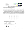
An example of preset values and values measured from a white object are shown in table
2.1, where a white sheet of paper was used as a white object for the measurements. The
“sunny” measurement was performed at 13:00, sky was clear and the object was fully
enlightened by sun. The “artificial” measurement was performed in a room with sealed
windows, with the object being lit by a single light bulb with no shield.
As one can see, artificial lighting tends to be more reddish, while flash light contains more
blue. Correct white balance setting can usually completely remove such colour biases.
Incorrect white balance settings lead to obvious colour biases, which can be reduced using
digital image processing software.
G/R
G/B
preset sunny
1.828
1.480
measured
sunny
1.820
1.355
preset flash
1.984
1.313
preset artificial
light
1.055
2.836
measured
artificial light
0.973
2.918
Table 2.1 – example values used for white balancing
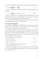
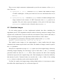
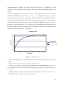
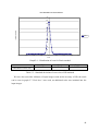
2.2.3 Colour scaling
The response of a CCD cell is linear to the amount of light that hits its surface. This is both
stated by the CCD manufacturers and confirmed by experiment we have performed. In this
experiment, we have taken pictures of a LCD screen with a certain percentage of pixels fully
lit, while others were fully black. We have gradually increased the number of lit pixels and we
have used optically blurred images (using an incorrect focal length), observing mean
measured value. As one can see from graph 2.1, the results confirm that the response is linear.
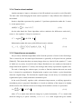
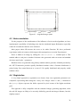
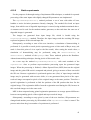
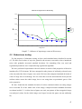
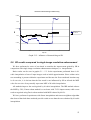
On the other hand, values stored in image files are not displayed linearly. This is a
commonly known fact, which was again confirmed by an experiment. Knowing that the
response of a CCD is linear, we have taken pictures of the LCD panel displaying image
containing increasing values of grey. Graph 2.2 shows the result, proving that values are
converted into light intensity exponentially. The reason for such behaviour of computer
display is based on the knowledge that the human eye perceives equal differences for equal
ratios of intensity of incoming light.
15
80%
70%
Measured response
60%
50%
Red
Green
Blue
40%
30%
20%
10%
0%
0%
10%
20%
30%
40%
50%
60%
70%
80%
90%
100%
Percent of lit pixels
Graph 2.1 – response of CCD. Measured values don’t reach 100% because of set
exposition value. Difference between measured channels is caused by non-white light source
and would be eliminated by correct white balancing.
90%
80%
measured light intensity
70%
60%
Red
50%
Green
40%
Blue
30%
20%
10%
0%
0%
10%
20%
30%
40%
50%
60%
70%
80%
90%
100%
gray value
Graph 2.2 – relation between grey value and light intensity
16
This knowledge implies a need for compensation when transforming values measured by a
CCD element into a computer image. Such compensation should be logarithmic, as later
exponential interpretation by computer display system will lead to linearity between original
measured light intensities and intensities produced by display system.
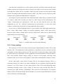
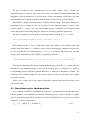
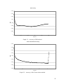
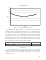
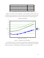
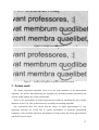
Figure 2.7 shows relationship between the measured values (y axes) and the values
contained in the final image (y axes). As one can see, this relationship is not single valued,
which is caused by used demosaicking algorithm, but the curve is generally logarithmic.
Figure 2.7 – Colour scaling – image gained by plotting points to positions horizontally
corresponding to measured value and vertically corresponding to value in image processed by
camera software.
2.3 Influence of pre-processing on SR algorithms
The current published SR algorithms are usually tested on simulated data. The reason for
this is that most of the algorithms are very sensitive to any noise in the input data. If we
consider that any interpolation, multiplication or other manipulation in computer suffers at
least from rounding errors, we can see that the original RAW data is the best possible input
for any SR method.
Moreover, many SR algorithms employ interpolation techniques. Such techniques may
suffer significantly when performed in non-linear space represented by the computer image
file.
We believe that using only exact measured values that are not affected by either
demosaicking, white balancing or colour scaling will lead to better results of SR algorithms
for real data. We may actually use SR instead of demosaicking, while we will need to apply
white balancing and colour scaling to the SR results manually to gain correct output images.
17
3. Resolution enhancement
Low resolution is one of the main downsides to the consumer level digital still cameras. An
obvious solution to this problem is using a higher-resolution CCD, but this is not always
acceptable for reasons which may include higher levels of noise contained in images taken by
high resolution CCD, high prices of such device or simple unavailability of a device that
could provide sufficient resolution.
Therefore, we would like to show ways of improving resolution of images above the
resolution of CCD used for capturing. The simplest way of doing so is resampling the image
to higher resolution. There exist numerous sophisticated algorithms providing high quality
results. Most of these algorithms are based on some interpolation technique, assuming point
sampling of input image, which is not the case of data produced by CCD images. Moreover,
all these methods are limited by the amount of information contained within the image (i.e.
there is no information about sub-pixel details of the original scene; such details cannot be
reconstructed from single image).
One way of adding more information to the resolution enhancement process is using
multiple images as input. These images may either contain different parts of the original scene
and simple (appropriate) merging of such images produces one image of the original scene
with resolution higher then the one of the CCD used to capture each image. Such an approach
is often used for taking pictures of large objects or panoramas.
It is not always possible to take pictures of parts of the scene at full resolution, as the
object may be, for example, too small for correct merging of partial images. Even in such case
an improvement of resolution using multiple input images may still be performed. Although
taking multiple images of an unchanged scene from the same position does not bring any new
information to the process, taking images shifted by sub-pixel (i.e. non-integer multiple of the
pixel size) distance will allow for considerable resolution enhancement.
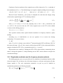
3.1 Super Resolution problem specification
Core of a problem denoted as super resolution lies within a simple idea, that multiple
slightly shifted images of unchanged scene contain more information than a single image, and
that such information could be exploited in order to increase the resolution of image.
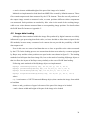
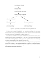
The validity of such assumption can be shown by the simple example in figure 3.1. Let us
suppose integral sampling of a function defined over continuous two-dimensional interval.
This function was sampled for the first time yielding for the first row values v11 = 1 and v12 =
18
0.5. Subsequently, the sampling mechanism was shifted to the right and sampling was
performed again, yielding values v11’ = 0.5 and v12’ = 1. In this example, one can see
(assuming values to be limited by 0 < v < 1) that the original function can be fully
reconstructed even though the sampling rate of both sampling procedures was below Nyquist
limit.
We can now define super resolution as a procedure, which takes as input multiple images
of unchanged scene, description of geometric warp between the images and other information
about the imaging process, and produces one image with resolution higher than resolution of
any of the input images. In most cases, super resolution is required to produce an image that
predicts well the input images being put through simulation of degradation process.
A procedure of gaining parameters of geometric warp between input images is denoted as
registration. Some of the methods presented include a special algorithm for registration,
whereas others rely on given information.
first sampling
second sampling
Figure 3.1 – Sampling example
3.2 Frequency domain methods
One of first attempts to solve the SR problem was presented in the work [Huang84] in
1984. A frequency domain approach was used, assuming that the original function was point
sampled. Discrete Fourier Transforms (DFTs) of the sampled data are then created and related
to each other via the shifting property. Subsequently DFT of the original image is constructed
and the original image is reconstructed via inverse Fourier transform.
Denote the original continuous scene by f ( x, y ) . Translated continuous images can then be
expressed as
f r ( x, y ) = f ( x + ∆x r , y + ∆y r ), r = 1,2,..., R
(3.1)
19
Continuous Fourier transform of the original scene will be denoted as F (u, v ) and that of
the translations as Fr (u , v) . The shifted images are impulse sampled yielding observed images
y r [m, n] = f (mTx + ∆x r , nT y + ∆y r )
where m=0,1,...,M-1 and n=0,1,...,N-1
(3.2)
Discrete Fourier Transform ( γ r [k , l ]) may be computed for each observed images, being
related to the original images CFT via aliasing relation:
γ r [k , l ] = α
∞
⎛ k
∞
∑ ∑ F ⎜⎜ MT
p = −∞ q = −∞
r
⎝
+ pf sx ,
x
⎞
l
+ qf sy ⎟
⎟
NT y
⎠
(3.3)
where fsx=1/Tx and fsy=1/Ty are the sampling rates in the x and y dimensions and
α = 1 / (TxT y ) . We can also relate the CFT of the original scene to the CFTs of the shifted
versions via the shifting property:
Fr (u, v ) = e j 2π ( ∆xr u + ∆yr v ) F (u , v )
(3.4)
This equation actually relates spatial domain translation to frequency domain as phase
shifting.
Assuming f(x,y) is band-limited, we can use equation 3.4 to rewrite the aliasing
relationship 3.3 in matrix form as
Y = ΦF
(3.5)
where Y is a R × 1 column vector with the rth element being the DFT coefficients γ [k, l ] of
the observed image y r [m, n] , Φ is a matrix which relates the DFT of the observation data to
samples of unknown CFT of f(x,y) contained in the 4LuLv × 1 vector F.
SR procedure now consists of finding the DFTs of the observed data, constructing the Φ
matrix, solving the equation 3.5 and performing inverse DFT on the solution to acquire the
reconstructed image.
3.2.1 Registration methods used for frequency domain methods
The shifting property gives us a powerful tool for estimation of translational motion within
observed images. We can choose one of the input images as a reference and register all other
images against it. The only registration parameters ∆x r and ∆y r can be handled as
optimization parameters of following formula:
[∆x , ∆y ] = arg Min( F (u, v ) − e
*
r
*
r
∆x , ∆y
r
j 2π ( ∆xr u + ∆y r v )
F (u, v )
)
(3.6)
20
For the real computation, equation 3.6 is used with the aliasing relation 3.3 to form an over
determined system of equations. Solving this equation system provides the desired
registration parameters.
3.2.2 Properties of frequency domain approach relevant to CCD sourced
images
There are two main drawbacks to this algorithm. First, it cannot be extended to handle
general motion including rotation. The shifting property can only handle translational motion
and there is no simple enough relation that would describe changes in frequency domain
caused by rotation in space domain.
The second important downside to this approach is that it assumes that the images are
point-sampled. In all current digital camera equipment it is much more accurate to assume for
integral sampling, as size of the light-sensitive cells is many times larger than the inter-cell
distances and the size of charge generated at each cell is related to integral of light that hits
whole area of the cell.
Because of these drawbacks, we will not take the frequency domain approach into account
in any further considerations.
3.3 Space domain methods
3.3.1 Unifying notation for space domain SR
Multiple methods for solving the super resolution problem in space domain were presented
exploiting various properties of the problem. One of these methods is Iterative Backprojection
(IBP), which will be described in detail later. Projection Onto Convex Sets (POCS) is another
space domain method which uses set theoretic approach to define convex sets which represent
constraints on required image. Probability theory was also used to define a space domain SR
method denoted as Maximum Aposteriori (MAP), where Bayesian framework is used to
maximize conditional probability of high resolution image.
As it is shown in [Elad97], all of the space-domain methods are closely related and may be
unified into a single SR method. This work also defines a new general notation for the SR
problem, which is used in most of the later research papers.
21
Images will be represented by lexicographically ordered column vectors, which will allow
representing most operations by matrix multiplication. Given N low resolution images are
denoted as
{Yk }kN=1
In general case, each image may be of different size [M k × M k ]. All of the low resolution
images are assumed to be representations of a single high resolution image X of size [L × L ] ,
where L > Mk for 1 ≤ k ≤ N . If we rewrite all images as column vectors, then this relation can
be represented by following formula
Yk = Dk C k Fk X + E k
for 1 ≤ k ≤ N
(3.6)
where:
[
]
Ck is a [L × L ] matrix representing blur in the degradation process
Dk is a [M × L ] matrix representing the decimation operator
Fk is a L2 × L2 matrix representing the geometric warp performed on the image X,
2
2
2
k
2
Ek is a column vector of length Mk2 representing additive noise.
The additive noise in this model can be generally any noise. Most of practical methods
assume the noise to be white Gaussian, although some methods exist to deal with non-white
noise. For the purposes of this work we will assume the noise to be white Gaussian and we
will later give some results of experiments we have performed to support this assumption.
3.3.2 Iterative Backprojection
Iterative Backprojection (IBP) is one of the most intuitive methods used to solve the SR
problem. It was first presented by [Peleg87] and it was adopted from Computer Aided
Tomography.
IBP employs an iterative algorithm, where each step takes current approximation of X and
all images Y as input and produces next approximation of X. In each step is for each input
image computed a simulated image from the current image and the original image degradation
parameters. Subsequently, the simulated image is compared to the original image and
resulting difference is back-projected onto the original image scale and position. Differences
(treated as errors) from all input images are finally averaged and subtracted from the original
image.
22
In the context of notation presented before, the requirement may be described as follows:
⎡N
⎤
X * = ArgMin ⎢∑ Dk H k Fk X − Yk ⎥
X
⎦
⎣ k =1
(3.7)
where X* is the solution we would like to find. The iterative algorithm then may be
expressed as:
⎡1
X n +1 = X n − β ⎢
⎣N
N
∑F
T
k
k =1
⎤
H kT DkT (Dk H k Fk X n − Yk )⎥
⎦
(3.8)
where β is a chosen step size. As starting approximation is usually used one of the input
images back-projected into the space of X. Iterating may be stopped after set number of
iterations or when the back-projected differences become insignificant.
In practical implementations matrix operations are usually replaced by image operations
such as shifting and blurring in order to reduce running times.
3.3.3 Zomet robust method
In [Zomet01], a modification of the IBP algorithm is presented, aiming to improve
robustness of the method. Robustness to noise in image data, to incorrect registration and to
outliers in input images should be improved by this method.
The algorithm is again based on iterative back-projecting differences between simulated
and given images and improving current approximation according to the results gained. The
basic difference between this algorithm and the IBP is in the way the errors are combined
together to be subtracted from the original image, where IBP uses mean of all error values for
each pixel and Zomet uses value of median.
The iteration process is expressed as follows:
X n +1 = X n + β∆L( X n )
(3.9)
where ∆L( X ) is defined as
∆L( X ) = median{Bk }k =1
n
(3.10)
where Bk represents difference gained from k-th image:
Bk = FkT H kT DkT (Dk H k Fk X n − Yk )
(3.11)
Relation to the IBP algorithm is obvious. The computational complexity is however higher,
as even sophisticated algorithms for finding median are more computationally complex than
linear computation of mean.
23
3.3.4 Farsiu robust method
Another attempt to improve robustness of the SR methods was made in work [Farsiu03].
The basic idea is that changing the norm used in equation 3.2 may influence the robustness of
the method.
Iterative algorithm represented by equation 3.2 performs optimization under the L2 norm,
i.e. mean squared error:
N
MSSE ( X ) = ∑ (Yk − Dk C k Fk X )
2
(3.12)
k =1
On the other hand, the Farsiu algorithm seeks to minimize the differences under the L1
norm, i.e. the equation 3.2 may be rewritten as:
⎡ n
⎤
X = ArgMin ⎢∑ Dk H k Fk X − Yk ⎥
X
1⎦
⎣ k =1
*
(3.13)
Minimization under this norm yields different iterative relation:
⎡N
⎤
X n +1 = X n − β ⎢∑ FkT H kT DkT sign(Dk H k Fk X n − Yk )⎥
⎣ k =1
⎦
(3.14)
3.3.5 Smoothness assumption
All previously mentioned algorithms suffer from the presence of noise in the final image.
This is caused by the fact that Super Resolution is generally an ill-posed inverse problem
[Baker02]. This means that there are many images that very closely fit the equation 3.7, some
of which are very noisy. In real life task of Super Resolution we are usually not interested in
images that fit the equation 3.7 exactly, but in images that closely represent the original scene.
The task of reducing the solution space, in order to find the solution that suits our needs
best, is denoted as regularisation. Regularisation requires some further a priori knowledge
about the original image. The fact that the original image was not noisy is a commonly used
regularisation prior, usually denoted as smoothness prior.
In the work [Farsiu03], together with a robustness improvement, a unifying approach to
smoothness priors is proposed. Smoothness is viewed as similarity of the image to its slightly
shifted version. The difference between an image and its shifted versions is expressed as:
P
P
D = ∑∑ α m +l X − S xl S ym X
(3.15)
l =0 m =0
where S xk is a matrix that shifts the image by k pixels horizontally, S yk is a matrix that
shifts the image by k pixels vertically, α : 0 < α < 1 is a scalar weight that gives smaller
24
effects to larger shifts and P is largest shift considered. The minimization task is then
expressed as
P P
⎡ n
⎤
X * = ArgMin ⎢∑ Dk H k Fk X − Yk + λ ∑∑ α m +l X − S xl S ym X ⎥
X
l =0 m =0
⎣ k =1
⎦
(3.16)
where λ is a scalar weighting the first term (SR similarity) to the second term (smoothness
regularization). With compliance to the idea presented in [Farsiu03], the equation (3.16) is
solved under a L1 norm, yielding iterative formula:
X n +1
⎡N T T T
⎤
⎢∑ Fk H k Dk sign(Dk H k Fk X n − Yk )
⎥
k =1
⎥
= Xn − β⎢
P P
⎢
⎥
m +l
l m
− m −l
I − S y S x sign(X − S x S y X )⎥
⎢+ λ ∑∑ α
⎣ l =0 m =0
⎦
[
]
(3.17)
3.3.6 Registration methods used for space domain SR
Space domain methods allow for much more general motion than frequency domain
methods. The Fk matrix in equation 3.6 can generally represent any type of motion and
general registration requires optimization of each of its elements.
In real task, usually the warp between images can be expressed by just a few parameters
(translation, rotation, sheering), according to which the Fk matrix is constructed. These
parameters can be optimised before the iterative task of spatial SR starts, relating all images to
the initial approximation. The optimisation may be expressed as
a * = arg Min[ Dk H k F (a )X 0 − Yk
]
(3.18)
a
where a is a vector of general registration parameters. Concrete solution of such
optimisation depends on the form of registration parameters.
In some research papers ([Elad98]), a very simple registration is used for the purposes of
demonstration of properties of SR algorithms without complicating the situation with complex
registration. A pure translational movement is assumed, and the size of the movement step is
limited to the size of cell of the high resolution grid. These assumptions simplify drastically
both registration and simulation of the degradation process, where the matrices Dk and Fk may
be represented by very simple image operations.
25
The registration itself is then performed as a search in a discrete space, a certain number of
registration parameters is searched to find a minimum according to equation 3.18 (i.e.
degradation process is simulated and such registration parameters are chosen that produce the
image closest to the one given as input).
In the work [Hard97], a further improvement is proposed, aiming to include information
from all input images to the registration process. Authors suggest not only to perform
registration once before the SR process starts, but also to refine the registration during the
process. In such case, the registration is performed against the current approximation, which
contains information from all input images. These refining steps may be taken after every
iteration of the SR algorithm, or only after a certain number of iterations.
The authors also suggest searching for improved registration parameters only within a
small area around the current ones, allowing for faster computation.
3.3.7 Properties of space domain approach relevant to CCD sourced
images
Both drawbacks of methods mentioned above are addressed by the space domain methods.
Using proper decimation matrix allows us to simulate integral sampling. The warp between
input images can take generally any form, which allows describing complex motion.
Nevertheless, assuming the motion to be simple simplifies the algorithms significantly,
allowing quick testing properties of algorithms that are not related to registration.
3.4 Improved algorithm derivation
In previous sections we have shown that an image captured by common digital still camera
undergoes complicated preprocessing that includes demosaicking, white-balancing and value
scaling. We have also shown that there are powerful algorithms capable of restoring a high
resolution image from multiple degraded and slightly shifted images. Now, we would like to
combine the knowledge acquired to propose an improved algorithm.
Our basic idea is that not all data contained within final image file are directly related to
the original scene. This is caused by the nature of demosaicking, which is basically
interpolating measured data. If such interpolated data could be removed from the SR process,
we believe it would have a positive effect on the result of any SR method.
Removal of interpolated data can be done in two ways, both of which assume knowledge
of concrete colour filter array layout. First possibility is to simply use only those R, G or B
values from the image file that was really measured. In this case we will be using values
26
altered by white-balancing, value scaling and in some cases also by demosaicking (some
algorithms even alter the measured values).
The other possibility is to use a camera capable of producing RAW data file. Such file only
contains values exactly measured by the CCD element, not altered by either of demosaicking,
white balancing or value scaling.
Any of the algorithms presented for the space domain SR can be used in almost unchanged
way. Each input image will only require a boolean mask that will tell the algorithm whether or
not to take the each pixel into account. Computation of the back-projected error can remain
unaltered, only using respectively lower number of input values.
It is possible that there will be areas of the image that were not measured by any of input
images. This leads original algorithms to keeping the values of first approximation at these
spots throughout the whole computation, which may be misleading. A better solution is
offered by incorporating the smoothness assumption presented above into the algorithm.
Doing so will effectively lead to interpolation of the current approximation for the spots not
measured by either of input images.
27
4. Implementation
This section focuses on the practical implementation of Super Resolution. The
implementation consists of three classes, all written in C#. This language was chosen because
it allows easy pure object programming, along with using the .NET Framework class library
routines for loading and saving images and because it does not show significant drop in
performance in comparison with lower level languages.
The data structure required for representing the images is implemented in the MyImage
class. Its data fields will be described first together with its basic constructors, while its
methods and advanced constructors will be described later, as they will become necessary.
The second class implemented is the SuperResolver class. This class provides methods
for the actual SR techniques together with some utility methods for generating testing images
and other support functions.
The last class represents a simple user interface, which allows using the previous classes to
super-resolve either artificially created inputs or real pictures.
4.1 Data structures
The basic data structure is represented by the MyImage object. It contains following data
fields:
•
double[,] pixels – two dimensional array of double values. Floating-point
number was chosen because the SR methods include floating-point operations and
rounding to integer value would introduce unnecessary errors. The values should be
always in the (0,1) interval, where 0 represents minimal amount of incoming light
and 1 represents maximum value (this usually relates to fully saturated CCD cell)
•
bool[,] mask – two dimensional array of binary values, that presents a mask,
marking pixels that are relevant to the image processing. This field is used to
distinguish between pixels of the image that were measured by the CCD (value
true) from the pixels computed by demosaicking (value false).
•
int w, h – integer values containing width and height of the image. These values
can be gained from the pixels array, but because they are used very often it is better
to access them in a quick and direct way.
•
int xs, ys – integer values used for registration. Their meaning will become clear
when registration will be described.
28
There are two simple constructors implemented to provide new instances of the MyImage
class. These are:
•
MyImage(int w, int h) – constructs a MyImage instance, that contains an image
of width w and height h. All the pixel values are set to zero and mask values are set
to false.
•
MyImage(Bitmap bmp) – constructs a MyImage instance of width and height of the
image contained in the instance of .NET Framework class Bitmap passed as an
argument. The pixel values represent brightness of the pixels of the input image
(GetBrightness method is used). All mask values are set to true.
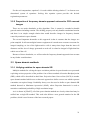
4.2 Simulated images
For the testing purposes we have implemented methods that allow simulating the
degradation process. This degradation includes neither of blurring, rotation or changes in the
original scene, and therefore it does not reflect the real situation exactly. On the other hand, it
allows considering properties of the algorithms without influence of these factors.
The degradation is performed by following member method of the MyImage class:
MyImage[] generateImages(int count, int rw, int ps)
This method creates images of size approximately ps-times smaller than the image
contained in the instance upon which it was called. The number of images created is equal to
the count parameter.
Each pixel is computed as average of ps x ps square area of the original image, effectively
simulating integral sampling. For each image a pair of shift values xs and ys is randomly
generated within the interval (-rw, rw). These values represent the shift of the sampling
mechanism expressed in the original image scale. Each sampling area is therefore shifted by
that amount of pixels. Generated values are stored in the xs and ys fields of the resulting
MyImage objects, so that they can be used as input for the SR.
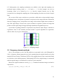
To allow for equally sized output images without blank borders, it is necessary to reduce
the width of the output images by 2rw, as shown in figure 4.1.
29
original image
xs=ys=0
xs=ys=rw
Figure 4.1 – degraded images spans
4.3 Noise simulation
For the purposes of the consideration of the influence of noise on the algorithms, we have
implemented a possibility of including noise into the simulated inputs. Robustness especially
cannot be considered without a noise inclusion.
Most papers about SR assume the noise to be white Gaussian. We have performed
experiments with real cameras which support this assumption (see section Experiments).
Noise is added to an image by calling the addNoise(double D) method upon it. This
method adds to each pixel a random Gaussian value generated with zero mean and standard
deviance equal to the D parameter.
Random values are generated using library random number generator. Method provided by
the .NET Framework provides equally distributed random values. Gaussian distribution is
gained using first central theorem as a sum of 120 equally distributed and properly scaled
random values.
4.4 Registration
A very simple approach to registration was chosen. Only two registration parameters are
computed, representing shifts along the x and y axes. Integer values xs and ys contained in
the MyImage objects represent the shifts expressed in pixel counts of the higher-resolution
grid.
This approach is fully compatible with the simulated images generating algorithm, while
the real-life images are likely to be not only shifted by general non-integer distance, but also
slightly rotated.
30
We have decided for this simplification for two main reasons. First, it makes the
registration process relatively easy, and second, most of available literature demonstrates SR
algorithms on such registration. It will be shown in the experiments section that even with
such simplification a significant quality improvement is gained for the real-life images.
Registration is always performed against a high resolution image. This image undergoes a
degradation process similar to the one described in the simulated images section, while
various values of xs and ys are used. The resulting image is compared to the input and shift
values that produce best fitting image are chosen as resulting registration parameters.
The basic registration is performed by following member method of MyImage class:
void registerSmall(MyImage hires, int width, int ps)
This method sets the xs and ys fields of the object upon which it was called to values that
produce best fit to image hires shifted by these values and integrally sampled with pixel size
ps. The algorithm tries all values from the (–width, width) interval and chooses the ones that
produce least Mean Squared Error (MSE), computed by function
double degMSE(MyImage aprox, int xsp, int ysp, int ps, bool useMask)
This function actually performs the same degradation process on the aprox image that was
described in the simulated images section. Each resulting pixel is compared to a pixel on
corresponding position and their squared difference is added to a summation variable. The
resulting value is finally computed as the sum of squared differences divided by the number
of compared pixels.
If the useMask flag is set to true, then the algorithm compares only pixels that have a true
value in the mask.
4.5 Smoothness prior implementation
As it is shown in [Hard97], smoothness prior plays a very important role in the SR process.
For the purposes of consideration of variable smoothing filters, we have decided to slightly
alter the theoretical approach to smoothness presented in [Farsiu03]. It is easy to see, that the
equation 3.17 may be rewritten as
X n +1 = X n − β SRT ( X n ) − βλ SMT ( X n )
(4.1)
31
where SRT(X) is a Super Resolution term and SMT(X) is a smoothness term. We have
altered this equation in a way which allows for very easy change of the used smoothness
prior, while it provides equal results to the equation 3.17:
X n +1 = X n − βSRT ( X n ) − βλ SMT ( X n − β SRT ( X n ))
(4.2)
This modification allows for sequential application of SR and smoothing, yielding:
X n +1 = X nSR − βλ SMT ( X nSR ) = SM ( X nSR , s )
(4.3)
where
X nSR = X n − βSRT ( X n ) is a result of SR improvement
SM(X,s) is a smoothing filter of strength s (in compliance with 3.17 s should be equal to
βλ ). We can now easily separate Super-Resolution from smoothing and replace smoothness
filter proposed by equation 3.17 by any filter providing better properties relevant to our task.
4.6 Implemented smoothing filters
All the smoothing filters implemented take one parameter that influences the strength of
the filter. This allows for simply changing of the filter used. Three filters were implemented,
the first one close to the original idea presented in [Farsiu03], the second one uses weighted
averaging of neighbouring pixels and the last one is aimed to improve the SR results by
preserving edges in the image.
4.6.1 Farsiu smoothing
This filter is close to the spirit of the smoothness prior proposed in [Farsiu03]. It practically
implements the smoothness term of the equation 3.17. The weighting parameter α is set to 0.5
and the width of the filter P is set to 2.
4.6.2 Weighted neighbourhood averaging filter
This filter sets a new value to every non-border pixel using the following equation
Px , y = (1 − s) Px , y +
s
s
s
s
Px +1, y + Px −1, y + Px , y +1 + Px +1, y −1
4
4
4
4
where s is the strength of the filter. Four D-neighbours are influencing the value of each
pixel, where the amount of influence is given by s.
32
4.6.3 Edge preserving smoothing filter
This filter was implemented in an attempt to create a filter that would both introduce
smoothness to the images, but also would not degrade sharpness of edges.
The algorithm considers all pixels in the 8-nighborhood of the smoothed pixel. First,
average value of all pixels in this neighbourhood with value larger than the value of the
smoothed pixel is computed. Similarly, average of all neighbouring pixel values smaller than
the one of the smoothed pixel is computed.
The final value of the pixel is set to weighted sum of its value and the value of the average
that is closer to the value of the pixel, i.e.:
Px , y = (1 − s) Px , y + sA+ / −
where s is the strength of the filter and A+/- is either average of larger or smaller
neighbouring pixels, depending on which is closer to the Px,y value.
4.7 Implemented SR methods
Three SR methods were implemented. All methods are based on the back-projection idea.
The first method is the classical IBP, the two remaining ones are methods aiming to improve
robustness of SR proposed by [Zomet01] and [Farsiu03].
All the methods work in an iterative manner, improving a starting approximation of high
resolution image. All the methods take the same set of arguments:
MyImage supRes(MyImage[] sources, bool doRegister, int ps, double beta,
double lambda)
where:
sources is the set of input images, each represented by one instance of MyImage object
doRegister
is a flag telling the method whether or not to attempt to register the input
images. If the flag is set to false, then the method uses registration parameters contained in the
input MyImage objects. If the flag is se to true, then the method alters the input images by
assigning new values to their registration data fields.
ps
(Pixel Size) is size of low-resolution grid pixel expressed by a number of high-
resolution grid pixels. In practice, value of ps tells the method the magnification factor by
which we want to improve the resolution.
beta
is size of step in the iterative process (see eq. 3.8). Optimal values will be discussed
later.
33
lambda
is strength of a smoothing filter applied to the image. The value actually
corresponds to the term βλ in equation 3.17. Optimal values will be also discussed later.
4.7.1 Iterated Backprojection
The first of the implemented methods is the Iterated Backprojection method that uses
minimization of the Mean Squared Error (MSE) between the input images and results of
degradation simulation performed on current approximation of the high resolution image.
The method first constructs a starting approximation of a high resolution image. For
images with full mask (i.e. with all mask positions set to true), a bi-cubic interpolation of the
first input image is used to gain an image of appropriate size. If there is used a mask
representing measured values of one of colours of Bayer array, then a demosaicking technique
is applied to the first input image before the bi-cubic interpolation is performed.
If the doRegister parameter is set to true, then the initial registration is performed by
calling the register method upon all the input images, passing the starting approximation as a
reference image.
Subsequently, a set number of improving steps is performed. It is shown in [Har97] that
IBP based methods converge to a solution in less than twenty steps, if the size of the step is
well chosen. Therefore we have decided that all the methods will use a constant number of
steps (40), which should ensure the convergence, and that we will find the size of step that
provides best results for this number of steps (see the Experiments section for results).
In each step, a following procedure is performed:
•
a difference image is computed for each input image, expressing difference
between the image and result of degradation simulation applied on the current
approximation
•
the differences are back-projected on the high resolution grid, taking into account
registration parameters of corresponding input images
•
an error image is computed by averaging pixel values of the difference images
•
the error image values are multiplied by the beta parameter
•
the error image is subtracted from the current approximation
Difference image is gained using a special MyImage constructor of following prototype:
MyImage(MyImage hires, MyImage lores, int ps)
where
hires is current approximation of the high resolution image
lores is one of input images
34
ps is size of pixel (magnification ratio)
This constructor returns image of difference between the input image and the high
resolution parameter degraded according to registration parameters contained within the
lores MyImage
object. The resulting image contains unprocessed difference, i.e. both positive
and negative values, and pixels of the image correspond to pixels of the given input image.
Note that the difference is only computed for pixels with mask set to true, while zero value is
left at positions of mask set to false.
This difference images are then backprojected to the high resolution image space. Two
arrays of size of high resolution image are created, one (named data) containing double
values which represent sum of errors, and other containing integer values (called counts)
representing number of pixels contributing to the sum. For pixels of every difference image
with mask set to true, a set of influenced high resolution pixels is found and value of the
difference is added to corresponding position of the data array, while the corresponding
elements of the counts array are incremented.
When this is done for all difference images, then the values of data array are divided by
corresponding values of the counts array, yielding array of average differences. The result is
put as data to a new instance of MyImage object called error. A method multiply(double m)
is called upon the error object, multiplying all the values by the beta parameter. Finally, the
error image is subtracted from the current approximation by calling the method
subtract(MyImage img)
upon the approximation MyImage object.
This process may generally lead to values outside the (0,1) interval. Therefore, the values
are clamped to fit in this interval by calling the clamp() method upon the high resolution
image object.
At this point, the high resolution image approximation corresponds to the XnSR element in
equation 4.3. A smoothing filter is now applied by calling one of methods that perform
smoothing.
Each iteration is finished by improving registration (only if the doRegister parameter is
set to true). The reRegister(...) method is called upon every input image, passing the
improved approximation as reference high resolution image. Smaller span of possible
registration parameters is being searched; a value of one fourth or one fifth of the original
registration width appears to provide good results while keeping the computation costs low.
35
4.7.2 Zomet robust method
Zomet robust method is implemented in a very similar way to the IBP method. First
approximation is gained in the same way, as well as the registration.
Each iteration of the algorithm consists of following steps:
•
computing the difference image
•
back-projecting the image to the high resolution grid
•
finding median value of the difference for each pixel of the high resolution grid
•
creating the error image from the pixel-wise median values
•
multiplying the error image by the beta parameter (size of step)
•
subtracting the error image from the approximation of the high resolution image
The difference image is computed in the same way as for the IBP method (see above).
Because we need to find median of the back-projected difference values, we must keep all of
them in a three-dimensional array called data (two spatial dimensions + third dimension for
storing multiple values for single pixel). The back-projection is performed in the same way as
for the IBP method, with the only difference, that the value is stored to the data array at
position [x,y,counts[x,y]] and the counts[x,y] value is incremented.
The median is now found in a simple way: Data for each pixel at position [x,y] are sorted
and value at position data[x,y,counts[x,y]/2] is put to the error image to position [x,y]. A
sorting method provided by .NET Framework Array class is used to perform the sorting.
The error image is treated in the same way as before. It is multiplied by the value of beta
and subtracted from the high resolution image. Image is clamped and filtered by one of
smoothing filters. Finally, registration is recomputed, reflecting last changes in the image.
4.7.3 Farsiu robust method
The Farsiu method also aims to improve robustness of the SR algorithm and is
implemented in a way similar to the previous algorithms. First, starting approximation is
created and all images are registered to it. The following steps are then iteratively repeated:
•
difference image is computed for every input image
•
sign function is applied to each difference image
•
results are back-projected to the high resolution grid
•
projections are averaged, forming the error image
•
error image is multiplied by the beta parameter
•
error image is subtracted from current approximation of the image
36
Difference images are gained in the way described above. Sign function is performed by
calling a method sign(double e) upon difference images. This method sets values in the
image according to following relation:
P’x,y
= -1
if Px,y < -e
=0
if -e <= Px,y < e
=1
if e <= Px,y
Although authors of [Farsiu03] suggest using pure sign function, our experiments showed
that including a possibility of result equal to zero in small neighbourhood of zero improves
significantly stability of the algorithm.
Back-projection is performed in the same way as it is done in the IBP algorithm, only a
sum is computed along with pixel count for each position. The error image then contains the
value of the sum divided by number of pixels at each position.
The following steps are performed in the same way as before, error is multiplied by beta
and subtracted from the high resolution image by calling the subtract method, image is
clamped a smoothed. Finally, registration parameters are recomputed using the
reRegister()
method.
4.8 RAW data loading
The methods for loading data from RAW data files were implemented as static methods of
the MyImage class returning new instance of MyImage class. These methods could be
implemented as constructors, but giving them names makes the source code more transparent.
In practical tasks the user usually does not want to super-resolve the whole image
contained within the RAW data file, because doing so would lead to excessive computational
requirements (for example a full 5 megapixel image super-resolved with pixel size of 3 leads
to a 45 megapixel image). Therefore the loading methods also allow specifying exact area of
the RAW image that should be loaded.
The loading methods have following prototypes:
MyImage RedFromMRW(string filename, int xs, int ys, int dw, int dh)
MyImage GreenFromMRW(string filename, int xs, int ys, int dw, int dh)
MyImage BlueFromMRW(string filename, int xs, int ys, int dw, int dh)
where:
filename is a string containing name of a RAW data file to be loaded
xs
and ys denote x and y positions of upper left corner of the part of the image to be
loaded
37
dw and dh denote width and height of the part of the image to be loaded
Methods are implemented to load data from MRW files created by Minolta cameras. These
files contain unprocessed data measured by the CCD element. Therefore not all positions of
the output image contain a measured value, at some positions different colour components
was measured. Such positions are marked by false value in the mask of the resulting image,
while a true value denotes measured data on corresponding image position. For details about
the RAW data file format see Appendix C.
4.9 Image data loading
Although the data contained within the image files produced by digital cameras are widely
influenced by pre-processing described earlier, we have decided to allow them as input for the
SR methods, because many consumer-level cameras do not provide the possibility of RAW
data output at all.
Even in this case we want to load data that are as close as possible to the values measured
by the CCD. In the loading process we assume that the data were taken by a camera equipped
by Bayer array and the colour positions are equal to the ones shown in figure 2.1. The loading
methods load all input data from image file, but set the mask of resulting MyImage object so
that it reflects the layout of the Bayer array similarly to the case of RAW data loading.
Following static methods of the MyImage object are implemented:
MyImage redFromImage(Bitmap bmp, int xs,int ys, int w, int h)
MyImage greenFromImage(Bitmap bmp, int xs,int ys, int w, int h)
MyImage blueFromImage(Bitmap bmp, int xs,int ys, int w, int h)
MyImage brightnessFromImage(Bitmap bmp, int xs,int ys, int w, int h)
where:
bmp
is an instance of .NET Framework Bitmap object, that contains the image from which
to load data
denote x and y positions of upper left corner of the part of the image to be loaded
w and h denote width and height of the part of the image to be loaded
38
Masks of resulting MyImage instances are created according to following expressions:
mask[nx,ny] = ((x + y) mod 2) == 1
for loading green
mask[nx,ny] = ((x mod 2) == 0) and ((y mod 2) == 0) for loading red
mask[nx,ny] = ((x mod 2) == 1) and ((y mod 2) == 1) for loading blue
where
nx and ny denote the position of the pixel within the cropped part of the image
x and y denote position of the pixel within the original image
Note that these expressions assume that the image was created from data gained using
Bayer array and that pixels of the image correspond exactly to Bayer-array cells shown in fig.
2.1. If the image was for example cropped by odd number of pixels before being set as input,
then these methods will load only values computed by demosaicking instead of loading the
least influenced values. Therefore we suggest using full images as input data and using
provided means of cropping to reduce the size of images.
The brightnessFrom(...) method loads brightness values from input file, using the
method getBrightness of the .NET Framework class Color. In this case, all mask pixels are
set to true.
4.10 Batch processing methods
For the purposes of easy usage of the software, two batch processing methods were
implemented. First of them encapsulates a process of super-resolving a RGB image, the other
allows for simple batch-experiments with methods applied on simulated data. Both of these
are methods of the user-interface object, and therefore both can access user interface elements
to gain required SR parameters.
4.10.1
Super-resolution of RGB images
Method SupresRGB() performs all steps needed to gain a RGB high resolution image from
either set of RAW data files or set of image files. This method is required because all
implemented SR methods work with single-valued data, while colour pictures require
processing of three colour components.
The method first loads green component of the input images and performs selected superresolution algorithm including registration. Subsequently, red and blue components are loaded
and super-resolution algorithm is applied without registration step. This both saves
39
computation time and makes the whole process more accurate, as registration of green
component is more accurate because there are twice more samples of green than either of red
or blue.
When all components are processed, a colour scaling is performed for the case of data
loaded from RAW data file. A method logaritmize() is called upon each MyImage instance
representing red, green and blue components. This method applies a logarithmic function to
each pixel value displaying values from linear space into logarithmic space. The parameters
of the logarithmic function were set so that the logarithmic function reflects as closely as
possible the curve shown in fig. 2.7 (the green curve was processed into a single-valued one
by using weighted average of possible values). The shape of this curve is compared to the
shape of the used logarithmic curve in graph 4.1.
Scaling curves
1
0,9
0,8
output value
0,7
0,6
measured values
0,5
computed curve
0,4
0,3
0,2
0,1
0
0
0,2
0,4
0,6
0,8
1
input value
Graph 4.1 – scaling curves
Finally, all components are combined together to form the resulting RBG image. A static
method
combine(MyImage red, MyImage green, MyImage blue)
of the MyImage class is used to perform quantization and combination into one Bitmap
object. Quantization is performed by multiplying the image values by 255 and converting to
int value.
Resulting bitmap is finally saved using function provided by the .NET Framework. A
lossless BMP format is used in order to get exact results.
40
4.10.2
Batch experiments
For the purposes of thorough testing of implemented SR techniques, a method for repeated
processing of the same inputs with slightly changed SR parameters was implemeted.
The DegradeAndSuperResolve() method performs a set of tests with either of beta,
lambda or noise deviation parameters linearly changing. The method first loads an input
image, from which a set of degraded input images is created, using methods mentioned above.
A constant seed is used for the random number generator, so that each time the same set of
degraded images is generated.
The images are generated from input image file, which is loaded using the
brightnessFromImage()
method. Therefore the input images and the resulting SR image
represent brightness of the selected input file.
Subsequently, according to state of the user interface, a simulation of demosaicking is
performed. It is possible to mask pixels representing green or blue mask of Bayer array (red
mask is from this point of view equal to the blue mask). After setting the mask values, a
simulation of demosaicking may be performed, using the demosaickGreen() or
demosaickBlue()
methods of the MyImage class. These methods perform the Hamilton-
Adams demosaicking technique, altering pixels of false mask value.
As a next step the method DegradeAndSuperResolve() calls static methods of the
SuperResolver
class to perform super-resolution processing upon the generated input
images. When the processing is finished, a Mean Squared Error (MSE) between the original
image and the gained SR result is computed and printed, giving a measure of how successful
the SR was. Because registration is performed against one (first) of input images and this
image may be generated with non-zero shifts, it is not guaranteed that pixels of the superresolved image correspond to pixels of the original image at the same position. Therefore a
special registration is performed to find the position of the SR product that best fits the
original image. This registration differs from the registration used during the SR, because in
this case both images are in the same scale.
MSE is then computed using gained registration parameters as average squared difference
between corresponding pixels of the original and super-resolved image.
Subsequently, according to setup given by state of the user interface, SR parameters are
changed and another processing by SR methods of the SuperResolver class is started. The
process ends when the given number of experiments is performed.
41
5. Experiments with simulated data
Multiple experiments were performed in order to compare and evaluate implemented SR
methods. We have decided to test three basic properties of each algorithm, which describe its
usability. These are accuracy, robustness and speed.
We will also test influence of demosaicking on results of SR, we will show that
demosaicking introduces error into this process and degrades the results and that removing
demosaicked pixels from the SR process improves its accuracy and performance.
We will compare results of SR methods to interpolation methods of enhancing resolution,
showing that SR provides considerable gain.
5.1 Accuracy testing
For the testing of accuracy, we have worked with simulated data. The input image (shown
in fig. 5.1) was degraded with pixel size 3 to form 20 input images for the SR methods.
Registration parameters were kept within small range (±5 pixels) in order to allow for fast
registration. No noise was introduced to the input images and no smoothing was performed
during SR. We have tried variable sizes of iteration step in order to gain a result with smallest
MSE.
Figure 5.1 – input image for the accuracy test, and its degraded version (3x magnified).
This image was chosen because it contains high frequencies that are usually lost by
degradation process.
Results of three experiments performed with three implemented methods are shown in
graphs 5.1, 5.2 and 5.3.
42
IBP accuracy
0,0016
0,0014
0,0012
MSE
0,001
0,0008
0,0006
0,0004
0,0002
0
0
0,01
0,02
0,03
0,04
0,05
0,06
step size
Graph 5.1 – accuracy of IBP method
Zomet robust method accuracy
0,0016
0,0014
0,0012
MSE
0,0010
0,0008
0,0006
0,0004
0,0002
0,0000
0
0,5
1
1,5
2
2,5
step size
Graph 5.2 – accuracy of the Zomet robust method
43
Farsiu robust method accuracy
0,0016
0,0014
0,0012
MSE
0,001
0,0008
0,0006
0,0004
0,0002
0
0
0,2
0,4
0,6
0,8
1
1,2
1,4
1,6
step size
Graph 5.3 – accuracy of the Farsiu robust method
These graphs show that MSE in dependency on step size develops in a similar way, first
dropping to a minimum and after the step size exceeds a certain value the MSE starts to rise
again. This behaviour is common for iterative algorithms and we have used these experiments
to gain optimal values of size of step. We have chosen values that both produce as low MSE
as possible, and also are not too close to the point where MSE starts to rise. This is especially
important for the Zomet method, where the values producing least MSE are very close to the
point where MSE rapidly rises. Table 5.1 shows the sizes of step we have found to produce
good quality results and which we have used for further experiments:
Method
IBP
Zomet robust
Farsiu robust
Size of step
0.025
1.4
0.76
Table 5.1 – step size values used for experiments, for results of SR using these parameters
see Appendix B
For the consideration of distribution of errors present in SR results we have computed
histograms of the error values for each method. Step sizes were chosen according to table 5.1,
histograms are shown in graphs 5.4-6. Standard deviations of the error sizes were also
computed in table 5.2.
44
Error distribution for IBP method
0,25
relative occurence
0,2
0,15
0,1
0,05
0
-0,08
-0,06
-0,04
-0,02
0
0,02
0,04
0,06
0,08
0,04
0,06
0,08
error
Graph 5.4 – Distribution of error for IBP
Error distribution for Zomet method
0,25
relative occurrence
0,2
0,15
0,1
0,05
0
-0,08
-0,06
-0,04
-0,02
0
0,02
error
Graph 5.5 – Distribution of error for Zomet method
45
Error distribution for Farsiu method
0,2
0,18
0,16
relative occurence
0,14
0,12
0,1
Řada1
0,08
0,06
0,04
0,02
0
-0,08
-0,06
-0,04
-0,02
0
0,02
0,04
0,06
0,08
error
Graph 5.6 – Distribution of error for Farsiu method
Deviation of error size
IBP
0,010074
Zomet
0,007467
Farsiu
0,010372
Table 5.2 – Standard deviations of error sizes of SR methods
We have also tested the influence of input images count on the accuracy of SR, the result
can be seen in graph 5.7. Pixel size 3 was used, no additional noise was included into the
input images.
46
Influence of image count on SR accuracy
0,003
0,0025
MSE
0,002
IBP
Zomet
Farsiu
0,0015
0,001
0,0005
0
0
2
4
6
8
10
12
14
16
18
20
Image count
Graph 5.7 – Influence of input image count on SR accuracy
5.2 Robustness testing
For the purposes of robustness testing we have used simulated noise described in section
4.3. We have used values of step size gained in the accuracy tests and we have introduced
noise with gradually increased standard deviation. No smoothing filter was used and
registration parameters were computed using registration algorithm.
We have performed experiments with real cameras in order to find properties of the noise
introduced by CCD elements. We have attempted to take pictures of uniformly coloured scene
(clear sky and white sheet of paper were used). We have then computed standard deviation of
values in large area of such image. We are aware that even the used materials do not provide
uniform colour across the whole image, but we are using these as pessimistic guess of the
noise properties.
We have found that the standard deviation of values contained within our testing images
never exceeded 2% of the whole scale of the image, example measured standard deviations
are shown in table 5.2. A white sheet of paper was used, one quarter of three megapixel image
was analyzed (values for the whole image were larger, because the paper was not uniformly
lit).
47
Standard deviation of red component
1,392%
Standard deviation of green component
1,477%
Standard deviation of blue component
1,026%
Standard deviation of brightness
1,175%
Table 5.2 – Standard deviation of values in picture of uniform coloured object
Based on the results of these experiments, we have decided to introduce noise with
standard deviation no larger than 2% of the scale, which for the MyImage representation leads
to maximum standard deviation of 0.02. Results of robustness tests are shown in graphs 5.8.
Robustness test of SR methods
0,0016
0,0014
0,0012
MSE
0,001
IBP
Zomet
Farsiu
0,0008
0,0006
0,0004
0,0002
0
0
0,002
0,004
0,006
0,008
0,01
0,012
0,014
0,016
0,018
0,02
Standard deviation of introduced noise
Graph 5.8 – Robustness tests of SR methods
An interesting fact can be seen on the Zomet method graph, showing that introducing small
amount of noise actually improved the performance of the method. Both other methods
behaved as expected, i.e. introducing noise caused growing of measured MSE.
48
5.3 Speed tests
We have performed several experiments aimed to analyse the speed properties of the
implemented algorithms. The running times were measured for experiments without
registration, with four sets of input parameters tested within each measurement. Various sizes
and counts of input images were used to test dependency on size of inputs. The result of the
experiment with various image sizes is shown in graph 5.9. Logarithmic scales are used, 20
input images of variable sizes were superresolved using implemented methods.
Results of testing of image count influence are shown in graph 5.10. The graph shows that
all running times depend linearly on the number of input images.
The tests with simulated data showed that Zomet robust method provides both accurate and
robust results, and even though its running times were longest of all methods we have decided
to use this method for further testing of impact of demosaicking and for experiments with real
images. On the other hand, the Farsiu method appeared to be less effective than the IBP in all
tests.
Speed tests
10000
running time [s]
1000
IBP
Zomet
Farsiu
100
10
1
10
100
1000
input image width [px]
Graph 5.9 – Speed tests with variable image sizes
49
Influence of input count
350
300
running time [s]
250
200
IBP
Zomet
Farsiu
150
100
50
0
0
5
10
15
20
25
30
35
number of input images
Graph 5.10 – Speed tests with variable input count
5.4 Smoothness tests
No smoothing was introduced into any of tests so far. Our experiments showed that for
exact data smoothing doesn’t improve performance. On the other hand, for input data
modified by additive noise smoothness filter provides considerable improvement. It is shown
in [Hard97] that SR without smoothness prior leads to noisy output images. We were testing
influence of smoothing filters applied during SR of simulated images in order to find optimal
strength of the filter.
We have used data with added noise of constant standard deviation value 0.02. We have
applied SR methods with step sizes from table 5.1. First, we have applied smoothing filter
proposed in section 4.6.2, results are shown in graph 5.11
50
Smoothness test
0,002
0,0018
0,0016
0,0014
MSE
0,0012
IBP
Zomet
Farsiu
0,001
0,0008
0,0006
0,0004
0,0002
0
0
0,02
0,04
0,06
0,08
0,1
0,12
0,14
0,16
0,18
0,2
Smoothness strength
Graph 5.11 – influence of smoothing filter on accuracy of SR methods
The graph shows that smoothness has positive effect on results of IBP (MSE reduced by
10%) and Zomet method (MSE reduced by 12%), while it does not help to improve result of
the Farsiu method. Optimal smoothing strength has for both IBP and Zomet method a value of
0.06, which will be used for real image testing.
We have performed experiments with methods starting with initial approximation gained
by linear interpolation or nearest neighbour algorithm. In these tests was improvement gained
by smoothness better, but overall MSE was always worse than the one of methods starting
with bi-cubic interpolation.
5.5 Influence of demosaicking on the SR process
We have performed a series of tests in order to consider influence of demosaicking on the
SR process. We have simulated the effects of demosaicking and compared results of SR that
considered all (i.e. both original and demosaicked) pixels to SR that considered only original
pixels. The image processing is described by figure 5.1.
51
Original image is loaded
pixels are masked
according to their
position within the Bayer array
masked pixels are recomputed
using demosaicking technique
All pixels are unmasked
SR method is performed
SR method is performed
results are compared
results are compared
to the original image
to the original image
Figure 5.1 – processing of images in the demosaicking influence test
We have used the same SR method for both cases shown in figure, for the reasons
discussed in the accuracy section the Zomet robust method was used. We have used variable
size of the iteration step, resulting MSEs are shown in graph 5.12.
The sudden rise of MSE for the selective method at step sizes between 0.5 and 1.0 is
probably caused by wrong registration. Even in such case are the results better than in than
results of SR considering all pixels. For the step size of 1.4 (which is chosen to be default step
size for the Zomet method) is MSE reduced by more than 50%.
The graph shows that influence of demosaicking onto the SR process is very negative. It is
obvious that it is better to omit the demosaicked values at the price of reducing amount of
input data, even for the better sampled green component. Similar results were obtained for the
blue component masking and demosaicking.
52
Influence of demosaicking on SR accuracy
0,0025
0,002
0,0015
MSE
Selective Zomet
Full Zomet
0,001
0,0005
0
0
0,5
1
1,5
2
2,5
step size
Graph 5.12 – influence of demosaicking on SR.
5.6 SR results compared to single image resolution enhancement
We have performed a series of test aimed to consider the improvement gained by SR in
comparison with single image resolution enhancement techniques, i.e. interpolations.
Basic results can be seen in graphs 5.1 – 5.3. In the experiments performed there is bicubic interpolation of one of input images used as initial approximation. Since neither noise
nor smoothing is present within the experiment and because the first considered iteration step
is of zero size, it is obvious that the first result is not influenced by SR at all and the MSE
value for zero size of step actually represents MSE of bi-cubic interpolation.
All methods improve the result gained by bi-cubic interpolation. The IBP method reduces
the MSE by 59%, Zomet robust method is even better with 76.2% improvement, while worst
result was gained using Farsiu robust method with MSE reduced by 40.8%.
We have performed experiments with linear interpolation and nearest neighbour algorithm
that showed that both these methods provide results worse than the ones obtained by bi-cubic
interpolation.
53
6. Experiments with real data
Multiple cameras were used for experiments with real data. We have tested multiple ways
of taking the picture (from hand, from tripod, from desk) and multiple ways of saving the
picture (raw data, image file). There is no way to globally measure success of SR, as original
image is not available. Therefore we present original images and SR results for subjective
consideration.
All the images were cropped, as super-resolution of full images leads to excessive
computational requirements. All original images shown here are magnified to the size of the
super-resolved results using nearest neighbour interpolation.
6.1 Images taken from camera held in hand
Image in figure 6.1 was taken by camera held in hand, no zoom was used. Camera
software was used for demosaicking. We have taken twelve such pictures, trying to avoid
rotating the camera. Nevertheless, the source images were slightly rotated (this was well
visible when images were viewed quickly one after another). Result of Zomet method is
shown in figure 6.2.
Figure 6.1 – source image
54
Figure 6.2 – Result of selective SR
6.2 Images taken from lying camera
Image in figure 6.3 was taken from camera lying on a hard table. The camera was slightly
rotated after each shot, which caused shifts of the images in x direction. The images were
taken at full optical zoom and the object was in cameras minimum focal distance, therefore it
was not possible to take any larger picture without changing imaging hardware. Image 6.3
shows one of the input images demosaicked by camera software.
Figure 6.3 – Image taken by camera lying on a table
Input images were processed by Zomet SR method, figure 6.4 shows result of full SR
taking into account both demosaicked and measured pixels, figure 6.5 shows result of SR
using only measured pixels.
55
Figure 6.4 – Result of SR by using all pixels
Figure 6.5 – Result of SR using measured pixels only
6.3 Images taken from tripod
We have taken series of pictures from tripod using studio lighting that allowed for very
short exposition times (1/600 s). Figure 6.6 shows one of input images, figure 6.7 shows the
result of Zomet SR.
56
Figure 6.6 – Image taken from tripod
Figure 6.7 – Result of SR applied on pictures taken from tripod
7. Future work
The simple registration algorithm seems to be the main drawback of the implemented
algorithm. We believe that improving the registration by including arbitrary translation and
rotation would enhance the results considerably.
There is also a possibility of further improving the results by simulating the inter-cellular
distances of the CCD. This could be done by extending our masking algorithm.
Our experiments have also shown that the choice of initial approximation is very
important, therefore we would like to explore possibilities of advanced interpolation
techniques, such as Radial Functions interpolation in both creating the initial approximation
and the SR process itself.
57
8. Conclusion
We have shown that data from digital still cameras undergo a complex processing before
they can be exported into some computer image format. We have described basic parts of this
processing, that includes demosaicking, white balancing and value scaling. We have
described multiple methods of demosaicking.
We have mentioned common resolution enhancement techniques of linear and bi-cubic
interpolation. We stated that resolution may be further improved by including multiple input
images of the unchanged scene. Two main approaches to this problem were discussed, the
frequency domain approach and the space domain approach. We have shown reasons why
space domain approach is more suitable for SR of images gained by CCD elements.
We have described general notation and three methods used for space domain SuperResolution. Smoothing prior and registration were discussed.
We have implemented the three methods of space domain SR along with utility functions
for creating images simulating data gained from a CCD element. We have thoroughly tested
implemented methods on both real and simulated data. We have found that the Zomet method
provides best results in both accuracy and robustness tests, but it is also slowest of all the
methods.
We have shown that demosaicking negatively influences the SR process. We have
improved the methods by introducing a mask to each of input images that separates measured
pixels from demosaicked ones. We have proven experimentally that removing demosaicked
pixels from registration a super-resolution improves the performance considerably.
Used abbreviations
CCD – Charge Coupled Device
IBP – Iterated Backprojection
SR – Super Resolution
MSE – Mean Squared Error
58
References
[Baker02] S. Baker, T. Kanade. Limits on Super-Resolution and How to Break Them.
2002
[Cok87] D. R. Cok. Signal Processing method and apparatus for producing interpolated
chrominance values in a sampled color image signal. U.S. Patent No. 4,642,678 (1987)
[Elad97] M. Elad, A. Feuer. Restoration of a Single Superresolution Image from Several
Blurred, Noisy, and Undersampled Measured Images. IEEE Transactions on Image
Processing, Vol. 6, No. 12, December 1997
[Elad98] M. Elad, Y. Hel-Or. A Fast Super-Resolution Reconstruction Algorithm for Pure
Translation Motion and Common Space-Invariant Blur. 1998
[Farsiu03] S. Farsiu, D. Robinson, M. Elad, P. Milanfar. Fast and Robust Super-Resolution.
2003
[Free88] W. T. Freeman. Median filter for reconstructing missing color samples. U.S.
Patent No. 4,724,395 (1988)
[Grant] K. Grant, D. Mould, M. Horsch, E. Neufeld. Enhancing Demosaicking Algorithms
using Loopy Propagation.
[Ham97] J. F. Hamilton, J. E. Adams. Adaptive color plane interpolation in single sensor
color electronic camera. U.S. Patent No. 5,629,734 (1997)
[Hard97] R. C. Hardie, K. J. Barnard, E. E. Armstrong. Joint MAP Registration and HighResolution Image Estimation Using a Sequence of Undersampled Images. IEEE
Transactions on Image Processing, Vol. 6, No. 12, December 1997
[Huang84] T. Huang, R. Tsai. Multi-frame image restoration and registration. In Huang,
T., editor, Advances in Computer Vision and Image Processing, volume 1, pages 317–339.
JAI Press Inc., 1984
[Laro94] C. A. Laroche, M. A. Prescott. Apparatus and method for adaptively
interpolating a full color image utilizing chrominance gradients. U.S. Patent No.
5,373,322 (1994)
[Peleg87] S. Peleg, D. Keren, L. Schweitzer. Improving image resolution using subpixel
motion. Pattern Recognition Letter, vol. 5, pp. 223-226, March 1987
[Skala93] V. Skala. Světlo, barvy a barevné systémy. Academia press, 1993
[Zomet01] A. Zomet, A. Rav-Acha, S. Peleg. Robust Super-Resolution. in Proceedings of
the Int. Conf. on Computer Vision and Pattern Recognition (CVPR), vol. 1, pp. 645-650,
Dec. 2001
59
Appendix A – User manual
Provided software consists of single executable file. It should run under any system
equipped with Microsoft .NET Framework, it was tested under Microsoft Windows XP. The
software does not require any special installation procedure, it may be simply copied to any
location.
The software does not have any hardware requirements above the ones of the operating
system and .NET Framework, although it may run out of memory for larger images and its
performance is influenced by power of processor used.
The program provides user interface that allows experiments with both real and simulated
images. The user interface consists of four boxes, where parameters of the desired process are
set. Figure A.1 shows example state of the user interface.
Figure A.1 – User interface
60
First of the boxes is marked with the “Method” label and allows selecting one of
implemented methods, using provided radio-buttons. This box also contains a checkbox
labelled “register”, which is used to set whether registration should be performed. These
settings are shared for both real and simulated data.
Second box is labelled “SR parameters” and allows explicit setting of used step size,
smoothness strength, registration width and pixel size (i.e. magnification coefficient). If the
checkbox “default values” is checked, then values of step size gained in section 5.1 and values
of smoothness strength gained in section 5.4 are used in correspondence with method selected
in the “Method” box.
Super resolution of real images is performed using the “Real images” box. It contains a list
of input files, to which new inputs may be added by clicking the “Add sources” button. Either
any image files supported by .NET framework (these include amongst others bmp and jpg
formats) or RAW data files may be selected. Combining image files with RAW data files is
not allowed.
The “Real images” box also provides tools for cropping input images, setting values to the
“X offset”, “Y offset”, “Width” and “Height” numeric boxes sets a window that will be used
as input for the SR. Finally, by clicking the “SuperResolve” button within the box a SR
process is started.
The “Simulated images” box provides controls for creating degraded versions of given
image and performing batch experiments with MSE evaluation. After the “Degrade and
SuperResolve” button is pressed, a dialog box appears asking the user to choose the input file.
A set of degraded images is generated from selected file, where number of the images can be
set in the “number of inputs” numeric field. Additional noise is added to each of the images
with standard deviation set by value in the “noise deviation” field.
Subsequently, generated images undergo processing by SR method selected in the
“Method” box. The processing is repeated according to number set in the “Number of
experiments” field, with all parameters are set according to the “SR parameters” box. Only
one selected parameter is changed between each experiment. One of step size, smoothness
strength and noise deviation may be changed, depending on which of the radio buttons is
selected. The value of the parameter is initially set to value contained in the “Initial value”
field, and after each experiment is value of the “Increment” field added.
After each experiment is the resulting image compared to the original image and their MSE
is printed to the output box. All other information about the progress of the SR process is also
displayed in the output box, both when real and simulated images are processed. As the
61
amount of information may be excessive for larger numbers of experiments, the user is
allowed to reduce the information displayed to only the final MSE by checking the “Reduced
output” checkbox within the “Simulated images” box.
A fact that processing is underway is signalized to the user by animation, messages in the
output box and the progress is shown by progress bar at the bottom of the window. Processing
can be stopped at any time by clicking the “Stop” button.
The program uses separate low-priority threads to run the computations, so that a computer
on which it runs can be simultaneously used for any other low resource-consuming task, like
word processing, without having to change the priority manually.
62
Appendix B – Results of SR of simulated images
Original image and its degraded version:
Results of SR with sizes of step from table 5.1. From the left: IBP, Zomet, Farsiu:
Results of the same SR methods applied to sources with additive noise of 0.02 std. deviation:
63
Results of same SR methods with applied smoothness filter with strength 0.06.
Image with simulated demosaicking, restored image using all inputs, restored image using
non-demosaicked pixels only.
64
Another example of SR results – landscape image. Original, degraded and superresolved
images are shown:
(More examples of superresolved images can be found on the attached CD in the
/examples folder)
65
Appendix C – MRW format description
Following text was taken from http://www.dalibor.cz/minolta/raw_file_format.htm in order
to provide information about concrete RAW file format.
Basic structure of .mrw file is here:
MRM Block
PRD Block
Picture Raw Dimensions
Here is a file format version, size of the image in pixels.
TTW Block
Tiff Tags W
This is a classic TIFF header with offset to IFDs containing
the TIFF tags, EXIF tags, PIM info, thumbnails,...
White Balance Gains
WBG Block Here are white balance coefficients measured when taking
the picture.
RIF Block
Requested Image Format
This block contains instructions for DIVU about how to create
a resulting image (sharpness, saturation, white balance, ...)
PAD Block
Zero PADding
Here are zeroes used to align the next block to 512 bytes
boundary. Therefore the maximum length of this block should
be 511 bytes with header.
Image Data
Here are the RAW image data read from CCD.
These are 16bit values of R, G, G' and B cells arranged in
lines.
Odd rows are RGRGRGRG...
Even Rows are GBGBGBGB...
Image Data
Every block in MRM (Minolta Raw M) has this structure:
Block Name
4 bytes
ex. 00 'M' 'R' 'M'
Block Length
4 bytes
big endian
(Mac style)
ex. 0x00007BF8
Block Data
misc data
see below
The length of whole block is then "Block Length" + 8.
66
0. MRM Block (Minolta Raw M)
This superblock contains all the rest blocks (except image data)
Name
Offset Size
Meaning
Block Name
0
4
Block name 00 'M' 'R' 'M'
Block Length
4
4
Length of the block
This is total length of all the rest blocks
Also this value + 8 is offset to RAW image data
Block Data
8
Here are stored blocks PRD, TTW, WBG, RIF and PAD
1. PRD Block (Picture Raw Dimensions)
All numbers are stored in big endian format (Macintosh/Motorola style). Offset is counted from start of
Block Data. This means that you have to add 8 to get offset from start of block. Size is in bytes.
Name
Offset
Size
Meaning
This number describes camera which has taken the picture
and therefore the version of raw file format.
27730001 for D5
27660001 for D7,D7u
27790001 for D7i
27780001 for D7Hi
Height of the image sensor (number of lines in Image Data)
1544 for D5
1928 for D7xx
Width of the image sensor (number of values in one line of
Image Data)
2056 for D5
2568 for D7xx
Height of the resulting image
1544 for D5 (probably a bug, it should be 1536)
1928 for D7 (probably a bug, it should be 1920)
1920 for D7u, D7i, D7Hi
Width of the resulting image
2048 for D5
2560 for D7xx
Version Number
0
8
CCD Size Y
8
2
CCD Size X
10
2
Image Size Y
12
2
Image Size X
14
2
Unknown1
16
2
0x100C = 4108
Unknown2
18
2
0x5200 = 20 992
Unknown3
20
2
0
Unknown4
22
2
1
67
2. TTW Block (Tiff Tags W)
This is a classic TIFF header as described in TIFF format specification ver. 6.0
Name
Offset Size
Meaning
MM is used in RAW (big endian, Macintosh/Motorola byte
order)
42 (You should know this number - "Life, Universe and
Everything...")
Byte order
0
2
Magic number
2
2
Offset of the first IFD
4
4
8 (right next data is the first (and the only) ImageFileDirectory)
IFD - Number of
entries
8
2
??? entries for D5
9 entries for D7
10 entries for D7u, D7i, D7Hi
IFD - Entry 1
10
12
Tag: Image Width (0x100)
IFD - Entry 2
22
12
Tag: Image Length (0x101)
IFD - Entry 3
34
12
Tag: Compression (0x103)
IFD - Entry 4
46
12
Tag: Image Description (0x10E)
IFD - Entry 5
58
12
Tag: Camera Make (0x10F)
IFD - Entry 6
70
12
Tag: Camera Model (0x110)
IFD - Entry 7
82
12
Tag: Software (0x131)
IFD - Entry 8
94
12
Tag: Date and Time (0x132)
IFD - Entry 9
106
12
Tag: EXIF IFD offset (0x8769)
IFD - Entry 9
118
12
Tag: PIM IFD offset (0xC4A5)
only for D7u, D7i, D7Hi
4
0 (this was the last IFD)
?
Here are the values of the tags described above
Offset of the next IFD
Values of tags
130
(or 118)
134
(or 122)
Description of EXIF tags can be found JEITA CP-3451 Standard
I do not know where to get a description of PIM tags. If you know it please let me know by e-mail.
Minolta MakerNote tag (part of EXIF) specification is not publicly available. I have decoded some parts
of it and I will publish its structure some day on my website.
68
3. WBG Block (White Balance Gains)
Name
White Balance R
denominator
White Balance G
denominator
White Balance G'
denominator
Offset Size
Meaning
Usually 2. Which means that you have to multiply the
white balance by 256.
0
1
2
1
4
1
White Balance B
denominator
0
1
White Balance R
2
2
White balance coefficient for channel R * denominator
White Balance G
4
2
White balance coefficient for channel G * denominator
White Balance G'
2
2
White balance coefficient for channel G' *
denominator
White Balance B
4
2
White balance coefficient for channel B * denominator
Other values have this meaning:
0 - 64
1 - 128
2 - 256
3 - 512
4 - 1024
Usually those coefficient are the same as those in MakerNote in EXIF. This is when G=G'=1.
But there are some shots where G and G's is not equal to one. In this case the MakerNote has
different white balance coefficients this time with G=1.
When user chooses in DIVU to use white balance as measured by camera the RAW image data are
multiplied by these white balance coefficients.
69
4. RIF Block (Requested Image Format)
Name
Offset Size
Meaning
Unknown
0
1
???
0 for D7, D7u
1 for D7i, D7Hi
Saturation
1
1
Saturation setting from -3 to 3
Contrast
2
1
Contrast setting from -3 to 3
Sharpness setting:
-1 for soft
0 for normal
1 for hard
White Balance setting:
0 for Camera Auto WB
1 for Daylight
2 for Cloudy
3 for Tungsten
4 for Fluorescent
Subject Program setting:
0 for None
1 for Portrait
2 for Text
3 for Night Portrait
4 for Sunset
5 for Sports Action
ISO speed value
This is a real ISO used by camera.
It is not limited to 100,200,400 and 800.
Here are the intermediate values like 109, 118, 154 too.
ISO = (2^((value/8.0)-1)*3.125)
Color Mode setting:
0 for Normal color
1 for black&white
2 for vivid color (D7i, D7Hi)
3 for solarization (D7i, D7Hi)
4 for AdobeRGB (D7Hi)
Sharpness
3
1
White Balance
4
1
Subject Program
5
1
Film Speed
6
1
Color Mode
7
1
Color Filter
56
1
Color Filter setting from -3 to 3
B&W Filter
57
1
B&W Filter value from 0 to 10 (can be non-zero even when
the picture was not taken in B&W mode)
Those values do not reflect camera setting when taking pictures. You can change them with DIVU
when you choose different setting for RAW file and save back (works only with DIVU 1, DIVU 2
doesn't save values back to RAW file.).
There are much more values but I was able to decrypt only those in the table. My problem is that I
have only a few raw files on my harddisk. If you have a large RAW collection and you are willing to
help with the rest please let me know.
70
5. PAD Block (Padding)
Here are just zeroes used to create a gap so that Raw Image Data start at 512 bytes boundary.
Raw Image Data
The rest of the file are RAW image data read from CCD.
They are stored sequentially in lines.
Length of the line is defined in PRD block.
The number of lines is in PRD block also.
Odd lines are RGRGRG..., even lines are GBGBGB...
Values are 12bit numbers stored in two bytes in big endian byte order.
There are eight pixels extra in horizontal and vertical directions.
They are lost when interpolating Bayer pattern.
71
Evidenční list
Souhlasím s tím, aby moje diplomová práce byla půjčována k prezenčnímu studiu
v Univerzitní knihovně ZČU v Plzni.
Datum: 21.5.2004
Podpis:
Uživatel stvrzuje svým čitelným podpisem, že tuto diplomovou/bakalářskou práci použil ke
studijním účelům a prohlašuje, že ji uvede mezi použitými prameny.
Jméno
Fakulta/katedra
Datum
Podpis
72