Download Proto Simulator User Manual

Proto Simulator User Manual
By the authors of MIT Proto
Last Updated: November 6, 2010
This is the user manual for the 2nd generation Proto simulator. For installation instructions, see the
README. For a reference of commonly used simulator and language commands, see the Proto Quick
Start. For a tutorial on the Proto language, see the document Thinking In Proto. For a reference to the
Proto language, see the Proto Language Reference. For information on how to extend the functionality
of the simulator, see the MIT Proto Developers Guide.
This manual is organized by functional modules within the simulator. For each module, there is a brief
description of the purpose and behavior of the module, followed by a list of the command-line arguments,
keys, and colors used by that module. Some modules conflict in arguments and keys. Ordinary keys are case
sensitive (i.e. c and C are different); control keys are case insensitive.
When arguments are described, an optional part of an argument is surrounded by square brackets: [].
Argument names always begin with a dash.
Bundled plugins also define additional sensor and actuator functions. These functions are described using
the same syntax as in the Proto Language Reference.
1
Credits for Proto
The Proto language was created in partnership by Jonathan Bachrach and Jacob Beal. As they created
the language, Jonathan created the first implementation of MIT Proto, including the first compiler, kernel,
simulator, and embedded device implementations. Since that time, Jake and other contributors have built
on the work begun by Jonathan.
MIT Proto also includes contributions from (alphabetically): Aaron Adler, Geoffrey Bays, Anna Derbakova, Nelson Elhage, Takeshi Fujiwara, Tony Grue, Joshua Horowitz, Tom Hsu, Kanak Kshetri, Prakash
Manghwani, Dustin Mitchell, Omar Mysore, Maciej Pacula, Hayes Raffle, Dany Qumsiyeh, Omari Stephens,
Mark Tobenkin, Ray Tomlinson, Kyle Usbeck, Dan Vickery
The Protobo platform code in platforms/protobo/ also includes Topobo-related code from (alphabetically): Mike Fleder, Limor Fried, Josh Lifton, Laura Yip
2
Default Argument Files
In addition to getting arguments from the command line the Proto simulator looks for files called .proto
in the current directory and your $HOME directory. The arguments in these files, if they exist, are added
to the end of the command line—first from the current directory, then from $HOME. Note that whitespace
and quotes are ignored in these files, as is any line beginning with “#”.
If you have created the simulator to have a non-standard name, it will search for .[thatname] instead.
3
Palette Files
All colors used by the simulator are user-controllable: their default values can be overridden with the use of
palette files.
1
Argument: -palette FILE
Loads the palette in FILE. This command can be invoked multiple times, loading multiple palettes.
Palettes load in the order they are specified on the command line, with later entries possibly
overriding earlier ones.
The simulator also always searches for a palette file named local.pal in the current directory. If this
file is found, it is loaded before any explicitly named palettes from the command line.
Palette files are formatted as follows:
• Whitespace is ignored
• “#” as first non-whitespace character in a line indicates a comment
• One color per line, specified NAME RED GREEN BLUE [ALPHA], where NAME is the name of the color, and
the others are values between zero and one. If unspecified, ALPHA defaults to 1.0, which is solid.
Each specified color replaces only the current value assigned to that color, so multiple palette files can be
layered, each changing only a portion of the colors.
Example Palette File:
# Turn the background a horrid pink
BACKGROUND 1 0.8 0.8 1
# Make the devices green and the times translucent cyan and white
SIMPLE_BODY 0 1 0
TIME_DISPLAY 0 1 1 0.5
FPS_DISPLAY 1 1 1 0.3
4
Core Simulator
The core functions of the simulator are to create a simulation, control its progress, and manage the user
interface.
If there is precisely one unhandled argument, that argument is taken to be the Proto script to run. If
there are no unhandled arguments, the script defaults to (app). If there are multiple unhandled arguments,
the simulator gives a warning and uses the last one as the script.
Argument: -seed N
Use N as a random seed, defaults to a value set by the current time.
Key: q
Quit the simulator.
Argument: -mag N
Relative magnification of text displays for each device, default 1.
Argument: -i, Key: i
Show the ID of each device (Color: DEVICE ID 1, 0, 0, 0.8). Toggled by key.
Starting, Stopping, and Running:
Argument: -T, Key: T
Display simulator time in lower left corner (Color: TIME DISPLAY 1, 0, 1, 1) and frames-persecond in lower right corner (Color: FPS DISPLAY 1, 0, 1, 1). Toggled by key.
2
Argument: -step, Key: s
Use stepping mode, advancing one step on key s
Key: x
Execute freely (ending stepping mode).
Argument: -stop-after N
Terminate after N simulated seconds, default infinity.
Argument: -throttle, Key: X
Throttle simulated time to advance relative to real time (toggled by key). When the simulator
cannot keep up, a warning appears in the lower center (Color: LAG WARNING 1, 0, 0, 1)
Argument: -ratio N
Ratio between real time and simulated time when throttling is active, default 1
Argument: -s N
Set simulated seconds per step, default 0.01/ratio
Key: CTRL-s
1
Slow throttled simulator. Each keystroke divides speed by 2 4
Key: CTRL-a
1
Accelerate throttled simulator. Each keystroke multiplies speed by 2 4
Key: CTRL-d
Return throttled simulator to a ratio of 1:1 simulated to real time.
Display:
The display background is colored (Color: BACKGROUND 0, 0, 0, 0.5).
Argument: -window-name NAME
Title the simulator window NAME, default “Proto Simulator”
Argument: -f, Key: f
Full screen display (toggled by key)
Argument: -headless
Run without a display or user interface; default FALSE unless compiled without OpenGL. When
headless, -stop-after must be specified.
Key: PAGE UP
Zoom in.
Key: PAGE DOWN
Zoom out.
Key: z
Reset display to initial view.
Key: ARROW KEYS
Shift simulation display in the direction of the arrow, in the simulation’s coordinate system.
Mouse: LEFT DRAG
Rotate display.
3
Mouse: RIGHT DRAG
Zoom display; toward center zooms out, away zooms in.
In addition, the display is produced using OpenGL and GLUT, and consumes a standard set of commandline arguments for that framework. Unlike other arguments, these arguments must come before the code to
be executed. Useful GLUT arguments include:
Argument: -display DISPLAY
Put simulator window on display device DIPLAY, defaulting to the current display.
Argument: -geometry WxH [+X [+Y]]
Size the siulator window to width W and height H, putting the top-left corner X pixels from the
left and Y pixels from the top. Defaults are 640x480 with corner at (100,100).
Selection: Selected devices are indicated with a thin ring (Color: DEVICE SELECTED 0.5, 0.5, 0.5, 0.8)
four times the device’s body diameter,
Mouse: LEFT CLICK
Select the devices clicked on.
Mouse: RIGHT CLICK
Select, then print the state of the selected device(s) to standard out.
Mouse: SHIFT LEFT DRAG
Toggle the selection of all devices in a rectangular display region. The area to be selected is
colored (Color: DRAG SELECTION 1, 1, 0, 0.5).
Mouse: SHIFT RIGHT DRAG
Move selected devices.
Key: U
Unselect all devices.
Code
Key: l
Recompile and reload the current script, injecting at the selected devices.
Argument: --path PATH
Add the directories in PATH to the front of the list of directories searched when looking for files (e.g.
Proto programs). By default, the path contains . (the current directory) and $libdir/proto/.
Argument: --basepath PATH
Override the default Proto path, substituting PATH instead.
Argument: --print-ast
During compilation, print out the intermediate abstract-syntax-tree form. Experimental: behavior may be flawed and may be changed without warning.
Argument: --instructions
After compiling, print the script instructions that have been generated, in the form of a C array
includable in a header file. Experimental: behavior may be flawed and may be changed without
warning.
4
Argument: -k, Key: k
Display the current script across the middle of the window (toggled by key). Not working!
Argument: -show-script-version, Key: j
Show what version of the script is loaded at each device (Color: DEVICE SCRIPT 1, 0, 0, 0.8).
Toggled by key.
Argument: -v, Key: n
Show value computed at each device (Color: DEVICE VALUE 0.5, 0.5, 1, 0.8). Toggled by key.
Argument: -sv, Key: v
When device outputs a 2- or 3-tuple, display it as a vector (toggled by key). The vector is
interpreted as meters, drawn as a line (Color: VECTOR BODY 0, 0, 1, 0.8) with a differently
colored tip to indicate direction (Color: VECTOR TIP 1, 0, 1, 0.8).
5
Plugins
The simulator is designed to be extensible with dynamically loadable plugins. This document assumes you
are just using plugins installed by user-friendly build packages. For more details on how the plugin system
works and where files live, see the MIT Proto Developers Guide.
The simulator can load three types of plugins, distributions, which determine how devices are scattered
through the initial volume of space (Section 8), time models, which determine when devices execute (Section 9), and layers, which modify the simulated environment in which the devices execute and add new
sensors, actuators, and other primitives.
Argument: --plugins
Display the inventory of available plugins that the simulator is able to find, then quit.
Argument: -DD DIST
Use the distribution named DIST.
Argument: -TM MODEL
Use the time model named MODEL.
Argument: -L LAYER
Incorporate the layer named LAYER into the simulation. This can be used multiple different times
to load different layers.
Argument: --DLL file
Attempt to load file as a plugin DLL. Adds system-appropriate extensions to the file name if
needed. This is option allows a developer to test a pluging without installing it.
The simulator requires certain sensors and actuators to be implemented, and uses default layers it they
are not implemented. If no physics model is loaded, it uses the SimpleDynamics physics simulator layer; if
no communication model is loaded, it uses the UnitDiscRadio layer; if no localization model is loaded, it
uses the PerfectLocalizer layer.
6
Debugging
The debugger logs chosen types of activity to standard out. To prevent complete overload, debugging
information flows only when global debug mode is on and then only from devices selected for debugging. In
that case, debugging information from designated categories prints to standard out from the devices selected
5
for debugging. Devices currently logging debugging information are shown by a filled disc twice the size of
the device (Color: DEVICE DEBUG 1, 0.8, 0.8, 0.5).
For example, to get a trace of networking activity in the kernel, add the command line arguments -g
-debug-kernel, then select the desired devices and hit D.
Key: D
Toggle selection for debugging on selected devices.
Argument: -g, Key: d
Global debug mode (toggled by key)
Argument: -t, Key: a
When debugging, post trace of evaluation in kernel of debug devices (toggled by key).
Argument: -debug-kernel
When debugging, post trace of networking activity in kernel
Argument: -debug-script
When debugging, post trace of viral code distribution in in kernel
7
State “Dumping”
The simulator can save “dumps” that contain a snapshot of the current state of every device in the simulator.
These snapshots produce Matlab-readable files. The first line is a Matlab comment containing the names of
all the state fields to be dumped; each subsequent line contains the state of a device, one number per field,
with fields separated by white-space.
The first three fields are always UID TICKS TIME, giving device ID, number of rounds executed, and
current time estimate.
Each simulator module has two arguments, -Dmodule and -NDmodule that assert that state for the module
must or must not be included in dumps, respectively. Some modules also have an argument -Dmodule-mask
that allows specific elements of its state to be included and excluded. The first element is enabled by the first
bit, the second by the second bit, and so on; these masks generally default to -1, meaning that all elements
will be included. These dumping arguments also control what information is printed when a device state is
printed to standard out, though that is printed more verbosely.
When a snapshot is taken, the screen flashes for 1/10 of a second (Color: PHOTO FLASH 1, 1, 1, 1).
Snapshot data is recorded in files named {STEM}{SIM TIME}.log for automatic dumps and {STEM}{REAL
TIME}-{SIM TIME}.log for dumps triggered by the user.
Argument: -no-dump-snaps
Don’t show a flash on dumps.
Key: Z
Dump a snapshot immediately.
Argument: -D, Key: 9
Enable periodic dumping of data. Disabled by default.
Key: 0
Disable periodic dumping of data.
Argument: -dump-after N
Start periodic dumping at time N, default 0.
6
Argument: -dump-period N
During periodic dumping, snapshot once every N seconds, default 1.
Argument: -dump-dir DIR
Store snapshot files in directory DIR, default dumps/. If the directory does not exist, it will be
created.
Argument: -dump-stem STEM
Start snapshot file names with STEM, default dump.
Positive Argument: -Dall, Negative Argument: -NDall
By default, are all modules included in dumps? Default TRUE.
Positive Argument: -Dhood, Negative Argument: -NDhood
Include neighborhood data in printed state, but not snapshot files (due to variability of size).
Positive Argument: -Dvalue, Negative Argument: -NDvalue
Include output value in dumps?
Argument: -probe-dump-filter, Key: 8
“Probe filtering” an unimplemented feature from the 1st generation simulator. Not working!
8
Device Distribution
Simulations are created with n devices distributed through a bounded 2D or 3D volume according to one of
several distribution rules.
Argument: -n N
Number of devices.
Argument: -3d
Use a 3D distribution; default is 2D.
Argument: -dim X [Y [Z]]
Set dimensions of expected volume where devices are to be located, centered at (0, 0, 0). Defaults
are X = 132, Y = 100, and Z = 0 (Z = 40 for 3D). Specifying a Z argument implies a 3D
distribution.
Devices are distributed through the expected volume unless otherwise specified by -dist-dim:
Argument: -dist-dim X- X+ Y- Y+ [Z- Z+]
Set bounds of initial device distribution (differing from expected volume). When the expected
volume is 3D, the Z arguments are required; when it is 2D they are prohibited.
By default, the distribution UniformRandom is used to place devices randomly through space. Several
other distributions are bundled with the Proto distribution:
Argument: -DD fixedpt X Y [Z]
Set the position of the first device (Z defaults to 0); all others are distributed uniformly randomly.
To set the position of more devices, follow with invocations of -fixedpt X Y [Z] used more
times, times the argument sets the position of more devices (e.g. the second use sets the position
of the second device).
7
Argument: -DD grid
Distribute devices in a grid that evenly fills the initial volume. If the grid does not divide evenly,
the rightmost row/plane will be incomplete.
Argument: -DD grideps EPSILON
Distribute devices in a grid as for -DD grid, but shift each device randomly in the range
[−/2, /2] for each coordinate.
Argument: -DD xgrid
Distribute X on a grid and Y randomly. If 3D, Z is distributed on a grid as well.
Argument: -DD hexgrid
Distribute devices on a hexagonal grid. If 3D, Z is distributed on a hexagonal grid as well.
Argument: -DD cylinder
Distribute devices uniformly randomly (using polar coordinates) on the surface of a cylinder
aligned with the X-axis, with diameter equal to the Y dimension of the initial volume.
Argument: -DD torus [RATIO]
Distribute devices unformly randomly (using polar coordinates) within a torus (or ring-shaped
band, if two-dimensional). The torus is aligned with the Z-axis, with outer diameter equal to
the minimum of the X and Y dimensions of the initial volume, and the central diameter equal to
RATIO times the outer diameter (default 0.75).
9
Device Time
Each device tracks its estimated time independently, executing the Proto program at regular intervals. The
relationship between device time and simulator time may vary, however.
The default time model, named FixedIntervalTime, takes the following arguments:
Argument: -sync
Synchronized execution of devices: no variation in rate or phase.
Argument: -desired-period P
Base number of device seconds between executions, default 1.
Argument: -desired-period-variance PV
Device periods are distributed randomly in the range [P − PV, P + PV], defaulting PV = 0.
Argument: -desired-ratio R
Base ratio between device time and simulator time, default 1.
Argument: -desired-ratio-variance RV
Device/simulator time ratios are distributed randomly in the range [R − RV, R + RV], defaulting
RV = 0.
10
Debugging I/O
The simulator always loads this layer, which provides simple sensors and actuators useful for demos and
debugging. The sensors are three boolean “user sensors” read by the Proto function (sense n), where
n is 1, 2, or 3. When TRUE, each sensor displays a disc four times the device size, colored (Color:
USER SENSOR 1 1.0, 0.5, 0, 0.8), (Color: USER SENSOR 2 0.5, 0, 1, 0.8), or (Color: USER SENSOR 3 1.0,
0, 0.5, 0.8) respectively.
8
The actuators are red, green, and blue LEDs, set by Proto functions (red value), (green value), and
(blue value), respectively. The LEDs may be shown independently as discs the size of the device body,
with colors (Color: RED LED 1, 0, 0, 0.8), (Color: GREEN LED 0, 1, 0, 0.8), (Color: BLUE LED 0, 0,
1, 0.8). Independent LEDs normally show their value both in intensity of color and Z displacement of the
LED disc above the device. LEDs may also be displayed mixed together into one double-sized disc with base
color (Color: RGB LED 1, 1, 1, 0.8), where the base color is scaled by LED values.
There are also three probes, which can expose intermediate values from evaluation. They display the
values as a tuple above each device in the positive Y direction (Color: DEVICE PROBES 0, 1, 0, 0.8).
Positive Argument: -Ddebug, Negative Argument: -NDdebug
Include debug layer data in dumps? Fields are: USER1 USER2 USER3 RED LED GREEN LED BLUE LED.
Argument: -Ddebug-mask MASK
Set which fields are included in dumps, default all (MASK = −1). Fields start at 0x2, not 0x1
(e.g. RED LED is controlled by 0x10) due to a removed field.
Argument: -probes N, Key: p
Display the first N of the three probes. The p key cycles through how many are shown.
Argument: -l, Key: L
Display LEDs (toggled by key).
Argument: -led-ghost, Key: 1
LED value controls transparency too, with 0 completely transparent and 1 completely opaque.
Toggled by key.
Argument: -led-flat, Key: 2
Do not use displacement in Z to show LED value. Toggled by key.
Argument: -led-stacking N, Key: 3
Set LED stacking to one of three modes. Mode 0 stacks LEDs directly, in order red, green, blue
bottom to top. Mode 1 sets heights independently, plus an offset of 1 meter for green and 2
meters for blue. Mode 2 sets heights independently. The 3 key cycles through the modes.
Argument: -led-blend, Key: 4
Show the LEDs as an RGB blend rather than independently. Toggled by key.
Key: t
Toggle user sensor 1 on selected devices.
Key: y
Toggle user sensor 2 on selected devices.
Key: u
Toggle user sensor 3 on selected devices.
Primitives
(red ,n|S)→ S
Set red LED to intensity n. Intensity ranges from 0 to 1, but overloading of display can show
values outside this range. The return echoes n.
(green ,n|S)→ S
Like red, except it acts on the green LED.
9
(blue ,n|S)→ S
Like red, except it acts on the blue LED.
(leds ,n|S)→ S
Set blue LED to (> n 0.25), green LED to (> n 0.50), and red LED (> n 0.75). The return
echoes n.
(rgb ,v|V )→ V
Set red, green, and blue LEDs to first, second, and third elements of v respectively. Extra
elements are ignored. The return echoes v.
(probe ,value|L ,i|S)→ L
Posts value to the ith probe (valid indices are 0 to 2).
(sense ,i|S)→ S
Returns the ith user sensor value.
(is-orange)→ B
Alias for (sense 1); in the simulator, this is a boolean displayed as an orange disc when true.
(is-purple)→ B
Alias for (sense 2); in the simulator, this is a boolean displayed as an purple disc when true.
11
11.1
Bundled Plugins
Unit Disc Radio Communication
Currently, the only communication model supported by the simulator is unit disc radio communication. In
this model, any pair of devices within a fixed radius r can communicate. While unit disc is only a coarse
approximation of real radio communication, it is a useful first approximation.
To speed up computation of neighbors, the devices are distributed into a grid of cells r in diameter. In
order to find its neighbors, a device thus needs only to search through adjacent cells.
The kernel has the option to decrease frequency of transmissions when nothing is changing in a node’s
outputs. Ordinarily it transmits every round, but when radio backoff is enabled, it increments its backoff
level b each transmission with unchanged values, setting the number of rounds between transmissions R to
R = d1.6b e
The backoff level is capped at 11, which gives R = 176. When values change, the backoff level goes back to
b = 0 immediately.
Positive Argument: -Dradio, Negative Argument: -NDradio
Include radio data in dumps? At present, however, no fields are dumped.
Argument: -debug-radio
When debugging, post neighbor decision-making process and display cell ID (Color: RADIO CELL INFO
0, 1, 1, 0.8).
Argument: -r N
Transmission range for radio, default 15.
Argument: -ns N
Set transmission range to get an expected neighborhood size of N. Overrides -r.
10
Argument: -txerr N
Probability of failure on message transmit, default 0.
Argument: -rxerr N
Probability of failure on message receive, default 0.
Argument: -no-motion-pruning
Ordinarily, moving devices delete neighbors that go out of range; this suppresses that behavior,
requiring them to time out instead.
Argument: -radio-backoff, Key: CTRL-x
Use exponential backoff of transmission frequency (toggled by key).
Display
Argument: -c, Key: c
Display network connections (toggled by key).
Argument: -sharp-connections, -sharp-neighborhood, Key: C
When network connections are displayed, the lines are drawn either thin and sharp (Color:
NET CONNECTION SHARP 0, 1, 0, 1) or thick and fuzzy (Color: NET CONNECTION FUZZY 0, 1,
0, 0.25). There are three modes: either all are fuzzy (default), all are sharp, or lines are sharp
where they connect to selected devices. The C key cycles through the three display modes.
Argument: -lc, Key: CTRL-c
Display “logical connectivity”—connections that are listed in a device’s neighborhood, whether
or not they currently exist. (Color: NET CONNECTION LOGICAL 0.5, 0.5, 1, 0.8)
Argument: -show-radio, Key: r
Display a ring around each device at its radio range. (Color: RADIO RANGE RING 0.25, 0.25,
0.25, 0.8)
Argument: -show-radio-backoff, Key: S
Display the current radio backoff level. (Color: RADIO BACKOFF 1, 0, 0, 0.8)
11.2
Simple Dynamics
The “simple dynamics” physics package evolves bodies based on their velocity, does not handle collisions,
and allows instantaneous shifts in velocity. The Proto function (mov vector) is used to set the velocity of
devices. In 2D, only the first 2 elements of the vector are used to actuate and devices are restricted to 2D
motion; in 3D the first three elements are used and devices move freely in 3D space. Simple dynamics is the
default physics package.
Bodies are shown as circles (Color: SIMPLE BODY 1, 0.25, 0, 0.8) when movement is enabled, points
when it is not.
Positive Argument: -Ddynamics, Negative Argument: -NDdynamics
Include dynamics data in dumps? Fields are: X Y Z V X V Y V Z RADIUS.
Argument: -Ddynamics-mask MASK
Set which fields are included in dumps, default all (MASK = −1).
Argument: -rad N
p
Radius of a device body, defaults from the initial distribution bounds: 0.087 ∗ (width ∗ height/n)
11
Argument: -h, Key: h
Show heading of a device with a tick on the body.
Argument: -S N
Maximum speed of devices, default 100.
Argument: -act-err N
Add a random actuation error of N times the size of the intended actuation.
Positive Argument: -w, Negative Argument: -nw, Key: w
Are there walls that repel devices from the edge of the initial distribution bounds? Default is
FALSE. The repulsive velocity is proportional to the distance into the wall zone, starting 80%
of the distance from the center of the bounds.
Argument: -floor
Include a “floor” at Z = 0 that 3D devices cannot move below.
Argument: -m, Key: m
Enable movement (toggled by key).
Argument: -hide-body, Key: b
Do not draw bodies (toggled by key).
Primitives
(radius)→ S
Return the estimated radius of the device’s body.
(radius-set ,r|S)→ S
Set the radius of the device’s body to r. The return echoes r.
11.3
ODE Dynamics
Not working!
The “ODE dynamics” physics package uses the Open Dynamics Engine[1], a free open-source Newtonian
physics simulator. ODE provides a high-quality simulation including collisions and joint physics. The Proto
function (mov vector) is used to set the desired velocity of devices, which then accelerate to try to maintain
that velocity.
Physics is always run in three dimensions, so “2D” means gravity and a floor, while “3D” means no
gravity and no floor. When there is a floor, it is set such that the center of a device is at Z = 0 when the
device is resting on the floor.
Device bodies are cubes (Color: ODE BOT 1, 0, 0, 0.7), with wire-box edges (Color: ODE EDGES 0, 0,
1, 1). When a device is selected, its color changes (Color: ODE SELECTED 0, 0.7, 1, 1). It is possible for
bodies in ODE to disable evolution, typically when a body is at rest and not interacting with other bodies.
If this happens, the color of the body changes (Color: ODE DISABLED 0.8, 0, 0, 0.7).
Walls are boxes; when visible they are (Color: ODE WALL 1, 0, 0, 0.1) with wire-box edges the same
color as device bodies. Walls, when present, are 10 meters thick, centered on the X-Y edges of the initial
distribution bounds, and extend in Z ten times the Y dimension of the pen. The corners have a 45-degree
wall 20 meters thick that smooths the corners of the pen.
Argument: -L ODE
Use ODE dynamics for physics.
12
Positive Argument: -Ddynamics, Negative Argument: -NDdynamics
Include dynamics data in dumps? Fields are: X Y Z V X V Y V Z Q 0 Q 1 Q 2 Q 3 W X W Y
W Z, where Q i is the quaternion specifying orientation and W i is the angular velocity.
Argument: -rad N
p
Radius of a device body, defaults from the initial distribution bounds: 0.087 ∗ (width ∗ height/n)
Argument: -density N
Density of device bodies, which determines mass. Default is 0.0625.
Argument: -S N
Maximum speed of devices, default 100.
Argument: -m, Key: m
Enable movement (toggled by key).
Argument: -hide-body, Key: b
Do not draw bodies (toggled by key).
Positive Argument: -w, Negative Argument: -nw, Key: w
Are there walls that pen devices into the initial distribution bounds? Default is FALSE.
Argument: -substep
Size of physics “microsteps” used by ODE, default 0.001. If too large, the simulation becomes
unstable and devices will fly off the screen.
Argument: -draw-walls
Display the walls, when there are walls.
Argument: -inescapable
If any device escapes the walls (when there are walls), put it back inside using the starting
distribution. If the starting distribution cannot supply another location, kill the device instead.
Argument: -rainbow-bots
Set device color by map device IDs onto hue, full saturation and value, alpha=0.7.
11.4
Simple Life Cycle
This layer allows devices to duplicate themselves or suicide. Duplication rate is limited by a cloning timer:
devices can only duplicate when the timer expires.
Argument: -L simple-life-cycle
Use the simple-life-cycle layer.
Positive Argument: -Dclone, Negative Argument: -NDclone
Include life cycle data in dumps? Fields are: CLONETIME (the time remaining before a clone can
be made).
Argument: -clone-delay N
Minimum number of seconds between duplications, default 1.
Key: B
Clone selected devices.
Key: K
Kill selected devices.
13
Primitives
(clone ,now|B)→ B
When now is true, the device attempts to reproduce. The return echoes now.
(die ,now|B)→ B
When now is true, the device attempts to suicide. The return echoes now.
11.5
Stop-When
This layer is designed for experiments where the end time is determined dynamically by the computation.
When enough devices have signalled true on their stop actuator, the simulator prints a message and exits.
Argument: -L stop-when
Use the stop-when layer.
Argument: -stop-pct N
Stop when N percent of nodes have signalled their stop actuator. Default 1.0.
11.6
Mote I/O
This layer represents the collection of sensor and actuator hardware that we have used on Mica2 Motes
at various times. There is one actuator (a speaker), four sensors (a light sensor, microphone, temperature
sensor, and short sensor), and two controls (a button and a slider). Of these, the 2nd generation simulator
only implements the button, which is drawn as a four-times radius disc (Color: BUTTON COLOR 0, 1, 0.5,
0.8).
Argument: -L mote-io
Use the Mode I/O layer.
Positive Argument: -Dmoteio, Negative Argument: -NDmoteio
Include Mote I/O data in dumps? Fields are: SOUND TEMP BUTTON.
Key: N
Toggle button on selected devices.
Primitives
(button ,i|S)→ B
Returns the current reading from the ith button. There are known bugs.
(light)→ S
Returns the current reading from a light sensor. Not working in 2nd generation simulator!
(sound)→ S
Returns the current sound level recorded by a microphone. Not working in 2nd generation
simulator!
(speak ,value|S)→ S
Feed value to a speaker. Not working in 2nd generation simulator!
(temp)→ S
Returns the current reading from a temperature sensor. Not working in 2nd generation simulator!
(conductive)→ B
Returns the current reading from a short sensor. Not working in 2nd generation simulator!
(slider ,dkey|S ,ikey|S ,init|S ,increment|S ,min|S ,max|S)→ S
Returns the current reading from a slider control. Not working in 2nd generation simulator!
14
11.7
Perfect Localizer
The only localizer implemented is a perfect localizer that supplies error-free device coordinates and velocity
in global coordinates. It has no controls.
Primitives
(coord)→ V3
Returns the device’s estimated coordinates.
11.8
Mote-link
The mote-link allows the simulator to interface with a network of Mica2 Motes, creating a mixed network of
real and simulated devices. It is not yet implemented for the 2nd generation simulator. When it is, it will
be invoked with the argument -motelink, and real devices will be drawn with (Color: MOTE BODY 1, 0, 1,
0.8).
11.9
Unimplemented First-Generation Primitives
These are primitives from miscellaneous experiments early in Proto’s history that have not yet been implemented in the second-generation simulator.
(grad-channel ,i|S)→ V
Ensure that chemical communication channel i is active and return a summary. Not working in
2nd generation simulator!
(new-channel ,alpha|S ,i|S)→ S
Set the diffusion constant of the ith chemical communication channel to be alpha. The return
echoes alpha. Note that the name and action of this function are not coherent. Not working in
2nd generation simulator!
(concentration ,i|S)→ S
Read the chemical concentration in the ith chemical communication channel. Not working in
2nd generation simulator!
(drip ,rate|S ,i|S)→ S
Increase the chemical in the ith chemical communication channel at rate. The return echoes r.
Not working in 2nd generation simulator!
(mouse)→ V2
Returns the current location of the mouse. Not working in 2nd generation simulator!
(ranger)→ V8
Returns the readout of an 8-way sonar rangefinder. Not working in 2nd generation simulator!
(cam ,i|S)→ S
Returns a camera reading. Not working in 2nd generation simulator!
(bump)→ B
Returns true if the device’s body is in contact with something. Not working in 2nd generation
simulator!
(local-fold ,active|B ,i|S)→ B
Interface to a folding actuator for surfaces like epithelial sheets. The boolean active indicates
whether the ith fold should currently be folding. The return echoes active. Not working in 2nd
generation simulator!
15
(fold-complete ,i|S)→ B
Interface to a folding actuator for surfaces like epithelial sheets. This returns true when the ith
fold is no longer moving. Not working in 2nd generation simulator!
References
[1] R. Smith, G. Carlton, F. Condello, N. Lin, M. C. Martin, T. Schmidt, K. Slipchenko, J. Smith,
V. Macagon, A. D. Moss, E. de Vries, N. Waddoups, and D. Whittaker. Open Dynamics Engine (version
0.7). http://www.ode.org, 2001 to 2006.
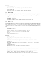
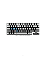
A
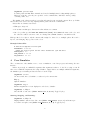
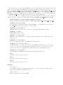
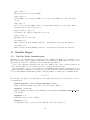
Keyboard Assignments:
Gray indicates reserved or unusable keys. Many keys are rendered unusable by the peculiarities of GLUT,
including its inconsistent implementation across platforms. Blue is allocated keys, pink is non-functional or
conflicting keys, and green is keys reserved for import of more 1st generation simulator functions.
‘
1
2
3
4
ghost
LEDs
flat
LEDs
LED
stacking
blend
LEDs
tab
q
w
quit
walls
e
8
9
r
t
y
u
i
sense 1
sense 2
sense 3
show id
s
d
f
step
debug
mode
full
screen
g
z
x
c
v
reset
display
execute
show
network
show
vector
alt
meta
ctrl
7
show
radio
a
shift
6
0
!
=
del
probe
enable
disable
dumping dumping dumping
trace
eval.
caps lock
esc
5
o
p
h
j
k
l
show
heading
script
version
show
script
load
script
b
show
bodies
n
m
show
value
motion
,
space
[
]
\
show
probes
;
.
’
return
/
shift
scroll
display
meta enter
Figure 1: Lower case keyboard assignments
~
!
tab
@
Q
#
W
$
E
%
^
R
T
&
Y
U
show
time
caps lock
shift
esc
ctrl
A
S
show
backoff
Z
X
snapshot
throttle
alt
D
F
debug
device
meta
*
(
I
O
C
G
V
P
+
{
del
}
|
unselect
H
J
K
B
N
clone
toggle
button
space
M
:
L
<
>
meta enter
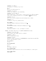
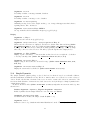
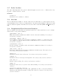
Figure 2: Upper case keyboard assignments
16
"
show
LEDs
kill
show net
sharp
_
)
?
return
shift
B
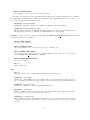
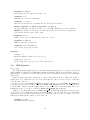
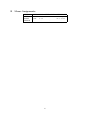
Mouse Assignments:
BUTTON
LEFT
RIGHT
MIDDLE
CLICK
select
print
—
DRAG
rotate
zoom
—
SHIFT-CLICK
—
—
—
17
SHIFT-DRAG
select region
move devices
—
‘
1
tab
Q
caps lock
shift
esc
2
ctrl
3
W
4
E
5
R
A
S
D
speed
throttle
slow
throttle
reset
throttle
T
F
Z
X
C
zoom
out
zoom in
/ backoff
logical
network
alt
meta
6
7
Y
G
V
8
U
H
B
space
I
J
N
9
O
K
M
!
0
P
,
.
meta enter
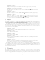
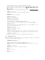
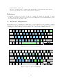
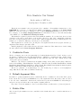
Figure 3: Control-key keyboard assignments
18
[
;
L
=
]
’
/
del
\
return
shift