Download Bibliographic References . . . . . . . . . . . . . . . . . . . . . . . . . . . . . . . 41 7

ii
MCSim User' Manual
6.4
6.5
6.6
6.7
6.3.3 OutputFile() specication : : : : : : : : : : : : : : : : : : : : : : : : : : : : : : 27
6.3.4 MonteCarlo() specication : : : : : : : : : : : : : : : : : : : : : : : : : : : : : : 27
6.3.5 Distrib() specication : : : : : : : : : : : : : : : : : : : : : : : : : : : : : : : : : 28
6.3.6 MCMC() specication : : : : : : : : : : : : : : : : : : : : : : : : : : : : : : : : : : : : : 30
6.3.7 SetPoints() specication : : : : : : : : : : : : : : : : : : : : : : : : : : : : : : : 32
Specifying basic conditions to simulate : : : : : : : : : : : : : : : : : : : : : : : : : : : 33
6.4.1 Experiment denition : : : : : : : : : : : : : : : : : : : : : : : : : : : : : : : : : : : 33
6.4.2 StartTime() specication : : : : : : : : : : : : : : : : : : : : : : : : : : : : : : : 34
6.4.3 Print() specication : : : : : : : : : : : : : : : : : : : : : : : : : : : : : : : : : : : 34
6.4.4 PrintStep() specication : : : : : : : : : : : : : : : : : : : : : : : : : : : : : : : 35
6.4.5 Data() specication : : : : : : : : : : : : : : : : : : : : : : : : : : : : : : : : : : : : : 35
Specifying a statistical model : : : : : : : : : : : : : : : : : : : : : : : : : : : : : : : : : : : : : 36
6.5.1 Level denition : : : : : : : : : : : : : : : : : : : : : : : : : : : : : : : : : : : : : : : : : 38
Analyzing results : : : : : : : : : : : : : : : : : : : : : : : : : : : : : : : : : : : : : : : : : : : : : : : : : 39
Error Handling : : : : : : : : : : : : : : : : : : : : : : : : : : : : : : : : : : : : : : : : : : : : : : : : : : : 40
Bibliographic References
7 Common Pitfalls
Appendix A Using make
Appendix B Examples
:::::::::::::::::::::::::::::::
::::::::::::::::::::::::::::::::::::
:::::::::::::::::::::::::::::::
::::::::::::::::::::::::::::::::
B.1
B.2
B.3
B.4
41
43
45
47
`linear.model' :: : : : : : : : : : : : : : : : : : : : : : : : : : : : : : : : : : : : : : : : : : : : : : : : :
`1cpt.model': A sample model description le : : : : : : : : : : : : : : : : : : :
`perc.model': A sample model description le : : : : : : : : : : : : : : : : : : :
`perc.lsodes.in' : : : : : : : : : : : : : : : : : : : : : : : : : : : : : : : : : : : : : : : : : : : : : : :
Concept Index
:::::::::::::::::::::::::::::::::::::::::::
47
47
49
54
55
i
Table of Contents
1 Software License
::::::::::::::::::::::::::::::::::::::
1
1.1 PREAMBLE : : : : : : : : : : : : : : : : : : : : : : : : : : : : : : : : : : : : : : : : : : : : : : : : : : : : : : 1
1.2 TERMS AND CONDITIONS FOR COPYING, DISTRIBUTION
AND MODIFICATION : : : : : : : : : : : : : : : : : : : : : : : : : : : : : : : : : : : : : : : : : : : : 2
2 Overview
::::::::::::::::::::::::::::::::::::::::::::::
7
2.1 General procedure : : : : : : : : : : : : : : : : : : : : : : : : : : : : : : : : : : : : : : : : : : : : : : : : : 7
2.2 Types of simulations : : : : : : : : : : : : : : : : : : : : : : : : : : : : : : : : : : : : : : : : : : : : : : 8
2.3 Major changes introduced with version 4.2.0 :: : : : : : : : : : : : : : : : : : : : : : 8
3 Installation
::::::::::::::::::::::::::::::::::::::::::::
9
3.1 System requirements : : : : : : : : : : : : : : : : : : : : : : : : : : : : : : : : : : : : : : : : : : : : : : 9
3.2 Distribution : : : : : : : : : : : : : : : : : : : : : : : : : : : : : : : : : : : : : : : : : : : : : : : : : : : : : : : 9
3.3 Machine-Specic Installation : : : : : : : : : : : : : : : : : : : : : : : : : : : : : : : : : : : : : : 9
4 Working Through an Example
5 Dening Models
:::::::::::::::::::::
:::::::::::::::::::::::::::::::::::::
11
13
5.1 Using Mod to process model description les : : : : : : : : : : : : : : : : : : : : : : 13
5.2 Syntax of the model description le : : : : : : : : : : : : : : : : : : : : : : : : : : : : : : : 13
5.2.1 General syntax : : : : : : : : : : : : : : : : : : : : : : : : : : : : : : : : : : : : : : : : : : 14
5.2.2 Global parameter declarations : : : : : : : : : : : : : : : : : : : : : : : : : : : 15
5.2.3 Special functions : : : : : : : : : : : : : : : : : : : : : : : : : : : : : : : : : : : : : : : : 16
5.2.4 Input functions : : : : : : : : : : : : : : : : : : : : : : : : : : : : : : : : : : : : : : : : : 17
5.2.5 Dynamics specications : : : : : : : : : : : : : : : : : : : : : : : : : : : : : : : : : 18
5.2.6 Parameter scaling : : : : : : : : : : : : : : : : : : : : : : : : : : : : : : : : : : : : : : : 19
5.2.7 Output calculations : : : : : : : : : : : : : : : : : : : : : : : : : : : : : : : : : : : : : 19
5.2.8 Comments on style : : : : : : : : : : : : : : : : : : : : : : : : : : : : : : : : : : : : : : 20
5.2.9 Note about models : : : : : : : : : : : : : : : : : : : : : : : : : : : : : : : : : : : : : : 21
6 Specifying Simulations
::::::::::::::::::::::::::::::
23
6.1 Using the compiled program :: : : : : : : : : : : : : : : : : : : : : : : : : : : : : : : : : : : : :
6.2 Syntax of the simulation denition le : : : : : : : : : : : : : : : : : : : : : : : : : : : :
6.3 Global specications : : : : : : : : : : : : : : : : : : : : : : : : : : : : : : : : : : : : : : : : : : : : :
6.3.1 SimType() specication : : : : : : : : : : : : : : : : : : : : : : : : : : : : : : : : :
6.3.2 Integrate() specication : : : : : : : : : : : : : : : : : : : : : : : : : : : : : : :
23
24
25
25
26
56
LogNormal v distribution : : : : : : : : : : : : : : : : : : : : : : : : : : 28
LogUniform distribution : : : : : : : : : : : : : : : : : : : : : : : : : : : 28
Lognormal distribution : : : : : : : : : : : : : : : : : : : : : : : : : : : : 28
Lsodes integrator : : : : : : : : : : : : : : : : : : : : : : : : : : : : : : : : : : 26
MCMC simulations : : : : : : : : : : : : : : : : : : : : : : : : : : : : : : : : : 8
MCMC() specication : : : : : : : : : : : : : : : : : : : : : : : : : : : : : 30
Major changes in versions 4.2.0 : : : : : : : : : : : : : : : : : : : : : : 8
Make : : : : : : : : : : : : : : : : : : : : : : : : : : : : : : : : : : : : : : : : : : : : : : 45
Markov-chain Monte Carlo simulations : : : : : : : : : : : : : 30
Mod syntax : : : : : : : : : : : : : : : : : : : : : : : : : : : : : : : : : : : : : : : : 13
Mod usage : : : : : : : : : : : : : : : : : : : : : : : : : : : : : : : : : : : : : : : : : 13
Model denition les : : : : : : : : : : : : : : : : : : : : : : : : : : : : : : : 13
Models : : : : : : : : : : : : : : : : : : : : : : : : : : : : : : : : : : : : : : : : : : : : 21
Monte Carlo : : : : : : : : : : : : : : : : : : : : : : : : : : : : : : : : : : : : : : : : 8
MonteCarlo() specication : : : : : : : : : : : : : : : : : : : : : : : : : 27
NDoses() function : : : : : : : : : : : : : : : : : : : : : : : : : : : : : : : : : 17
Normal cumulative density function : : : : : : : : : : : : : : : : 16
Normal density function : : : : : : : : : : : : : : : : : : : : : : : : : : : 16
Normal distribution : : : : : : : : : : : : : : : : : : : : : : : : : : : : : : : : 28
NormalRandom() function : : : : : : : : : : : : : : : : : : : : : : : : : 16
Normal v distribution : : : : : : : : : : : : : : : : : : : : : : : : : : : : : : 28
Output specication : : : : : : : : : : : : : : : : : : : : : : : : : : : : : : : 19
Output variables : : : : : : : : : : : : : : : : : : : : : : : : : : : : : : : : : : : 15
OutputFile() specication : : : : : : : : : : : : : : : : : : : : : : : : : : 27
Overview : : : : : : : : : : : : : : : : : : : : : : : : : : : : : : : : : : : : : : : : : : : 7
Parameter declaration : : : : : : : : : : : : : : : : : : : : : : : : : : : : : 15
Parameter scaling : : : : : : : : : : : : : : : : : : : : : : : : : : : : : : : : : : 19
PerDose() function : : : : : : : : : : : : : : : : : : : : : : : : : : : : : : : : : 17
PerExp() function : : : : : : : : : : : : : : : : : : : : : : : : : : : : : : : : : 17
Piecewise distribution : : : : : : : : : : : : : : : : : : : : : : : : : : : : : : 28
Pitfalls : : : : : : : : : : : : : : : : : : : : : : : : : : : : : : : : : : : : : : : : : : : : 43
Poisson distribution : : : : : : : : : : : : : : : : : : : : : : : : : : : : : : : : 28
Print() specication : : : : : : : : : : : : : : : : : : : : : : : : : : : : : : : : 34
PrintStep() specication : : : : : : : : : : : : : : : : : : : : : : : : : : : 35
Random number, normal : : : : : : : : : : : : : : : : : : : : : : : : : : : 16
Random number, uniform : : : : : : : : : : : : : : : : : : : : : : : : : : 16
Scale, scaling specication : : : : : : : : : : : : : : : : : : : : : : : : : 19
MCSim User' Manual
Semi-colon : : : : : : : : : : : : : : : : : : : : : : : : : : : : : : : : : : : : : : : : : 14
SetPoint() specication : : : : : : : : : : : : : : : : : : : : : : : : : : : : 32
SetPoints simulations : : : : : : : : : : : : : : : : : : : : : : : : : : : : : : : 8
SimType() specication : : : : : : : : : : : : : : : : : : : : : : : : : : : : 25
Simulation denition les : : : : : : : : : : : : : : : : : : : : : : : : : : 23
Simulation le, syntax : : : : : : : : : : : : : : : : : : : : : : : : : : : : : 24
Software license : : : : : : : : : : : : : : : : : : : : : : : : : : : : : : : : : : : : : 1
Special functions : : : : : : : : : : : : : : : : : : : : : : : : : : : : : : : : : : : 16
Specication, Data() : : : : : : : : : : : : : : : : : : : : : : : : : : : : : : : 35
Specication, Distrib() : : : : : : : : : : : : : : : : : : : : : : : : : : : : : 28
Specication, Integrate() : : : : : : : : : : : : : : : : : : : : : : : : : : : 26
Specication, MCMC() : : : : : : : : : : : : : : : : : : : : : : : : : : : : 30
Specication, MonteCarlo() : : : : : : : : : : : : : : : : : : : : : : : : 27
Specication, OutputFile() : : : : : : : : : : : : : : : : : : : : : : : : : 27
Specication, Print() : : : : : : : : : : : : : : : : : : : : : : : : : : : : : : : 34
Specication, PrintStep() : : : : : : : : : : : : : : : : : : : : : : : : : : 35
Specication, SetPoint() : : : : : : : : : : : : : : : : : : : : : : : : : : : 32
Specication, SimType() : : : : : : : : : : : : : : : : : : : : : : : : : : : 25
Specication, StartTime() : : : : : : : : : : : : : : : : : : : : : : : : : : 34
Specication, statistical model : : : : : : : : : : : : : : : : : : : : : 36
Specifying simulations : : : : : : : : : : : : : : : : : : : : : : : : : : : : : 23
Spikes() function : : : : : : : : : : : : : : : : : : : : : : : : : : : : : : : : : : : 17
StartTime() specication : : : : : : : : : : : : : : : : : : : : : : : : : : : 34
State variables : : : : : : : : : : : : : : : : : : : : : : : : : : : : : : : : : : : : : 15
Statistical model specication : : : : : : : : : : : : : : : : : : : : : : 36
Style : : : : : : : : : : : : : : : : : : : : : : : : : : : : : : : : : : : : : : : : : : : : : : 20
Syntax for mod : : : : : : : : : : : : : : : : : : : : : : : : : : : : : : : : : : : : 13
Syntax of simulation les : : : : : : : : : : : : : : : : : : : : : : : : : : 24
Triangular distribution : : : : : : : : : : : : : : : : : : : : : : : : : : : : : 29
TruncLogNormal distribution : : : : : : : : : : : : : : : : : : : : : : 28
TruncLogNormal v distribution : : : : : : : : : : : : : : : : : : : : 28
TruncNormal distribution : : : : : : : : : : : : : : : : : : : : : : : : : : 28
TruncNormal v distribution : : : : : : : : : : : : : : : : : : : : : : : : 28
Uniform distribution : : : : : : : : : : : : : : : : : : : : : : : : : : : : : : : 28
UniformRandom() function : : : : : : : : : : : : : : : : : : : : : : : : 16
Unix make utility : : : : : : : : : : : : : : : : : : : : : : : : : : : : : : : : : : 45
Working Through an Example : : : : : : : : : : : : : : : : : : : : : 11
Concept Index
55
Concept Index
'#' sign : : : : : : : : : : : : : : : : : : : : : : : : : : : : : : : : : : : : : : : : : : : 14
';' sign : : : : : : : : : : : : : : : : : : : : : : : : : : : : : : : : : : : : : : : : : : : : : 14
Analyzing results : : : : : : : : : : : : : : : : : : : : : : : : : : : : : : : : : : 39
Assignment : : : : : : : : : : : : : : : : : : : : : : : : : : : : : : : : : : : : : : : : 14
Beta distribution : : : : : : : : : : : : : : : : : : : : : : : : : : : : : : : : : : 28
Bibliographic references : : : : : : : : : : : : : : : : : : : : : : : : : : : : 41
Binomial distribution : : : : : : : : : : : : : : : : : : : : : : : : : : : : : : 28
Blank lines : : : : : : : : : : : : : : : : : : : : : : : : : : : : : : : : : : : : : : : : 14
CDFNormal() function : : : : : : : : : : : : : : : : : : : : : : : : : : : : : 16
CalcOutputs, output specication : : : : : : : : : : : : : : : : : : 19
Chi2 distribution : : : : : : : : : : : : : : : : : : : : : : : : : : : : : : : : : : 28
Colon conditional assignment : : : : : : : : : : : : : : : : : : : : : : 14
Comments : : : : : : : : : : : : : : : : : : : : : : : : : : : : : : : : : : : : : : : : : 14
Common pitfalls : : : : : : : : : : : : : : : : : : : : : : : : : : : : : : : : : : : 43
Comparison operators : : : : : : : : : : : : : : : : : : : : : : : : : : : : : : 15
Conditional assignment : : : : : : : : : : : : : : : : : : : : : : : : : : : : 14
Cumulative density function, Normal : : : : : : : : : : : : : : : 16
Data() specication : : : : : : : : : : : : : : : : : : : : : : : : : : : : : : : : 35
DefaultSim : : : : : : : : : : : : : : : : : : : : : : : : : : : : : : : : : : : : : : 8, 25
Dening models : : : : : : : : : : : : : : : : : : : : : : : : : : : : : : : : : : : 13
Density function, Normal : : : : : : : : : : : : : : : : : : : : : : : : : : 16
Derivative specication : : : : : : : : : : : : : : : : : : : : : : : : : : : : 18
Distrib() specication : : : : : : : : : : : : : : : : : : : : : : : : : : : : : : 28
Distribution, Poisson : : : : : : : : : : : : : : : : : : : : : : : : : : : : : : : 28
Distribution, beta : : : : : : : : : : : : : : : : : : : : : : : : : : : : : : : : : : 28
Distribution, binomial : : : : : : : : : : : : : : : : : : : : : : : : : : : : : 28
Distribution, chi2 : : : : : : : : : : : : : : : : : : : : : : : : : : : : : : : : : : 28
Distribution, exponential : : : : : : : : : : : : : : : : : : : : : : : : : : : 28
Distribution, gamma : : : : : : : : : : : : : : : : : : : : : : : : : : : : : : : 28
Distribution, inverse-gamma : : : : : : : : : : : : : : : : : : : : : : : 28
Distribution, lognormal v : : : : : : : : : : : : : : : : : : : : : : : : : : 28
Distribution, lognormal : : : : : : : : : : : : : : : : : : : : : : : : : : : : 28
Distribution, loguniform : : : : : : : : : : : : : : : : : : : : : : : : : : : 28
Distribution, normal v : : : : : : : : : : : : : : : : : : : : : : : : : : : : : 28
Distribution, normal : : : : : : : : : : : : : : : : : : : : : : : : : : : : : : : 28
Distribution, piecewise : : : : : : : : : : : : : : : : : : : : : : : : : : : : : 28
Distribution, triangular : : : : : : : : : : : : : : : : : : : : : : : : : : : : 29
Distribution, truncated lognormal : : : : : : : : : : : : : : : : : : 28
Distribution, truncated normal : : : : : : : : : : : : : : : : : : : : : 28
Distribution, trunclognormal v : : : : : : : : : : : : : : : : : : : : : 28
Distribution, truncnormal v : : : : : : : : : : : : : : : : : : : : : : : : 28
Distribution, uniform : : : : : : : : : : : : : : : : : : : : : : : : : : : : : : 28
Dt() operator : : : : : : : : : : : : : : : : : : : : : : : : : : : : : : : : : : : : : : 18
Dynamics specications : : : : : : : : : : : : : : : : : : : : : : : : : : : : 18
Erfc() function : : : : : : : : : : : : : : : : : : : : : : : : : : : : : : : : : : : : : 16
Error function : : : : : : : : : : : : : : : : : : : : : : : : : : : : : : : : : : : : : 16
Error handling : : : : : : : : : : : : : : : : : : : : : : : : : : : : : : : : : : : : : 40
Euler integrator : : : : : : : : : : : : : : : : : : : : : : : : : : : : : : : : : : : : 26
Examples : : : : : : : : : : : : : : : : : : : : : : : : : : : : : : : : : : : : : : 13, 47
Experiment denition : : : : : : : : : : : : : : : : : : : : : : : : : : : : : : 33
Exponential distribution : : : : : : : : : : : : : : : : : : : : : : : : : : : 28
Function, CDFNormal() : : : : : : : : : : : : : : : : : : : : : : : : : : : 16
Function, NDoses : : : : : : : : : : : : : : : : : : : : : : : : : : : : : : : : : : 17
Function, NormalRandom() : : : : : : : : : : : : : : : : : : : : : : : : 16
Function, PerDose() : : : : : : : : : : : : : : : : : : : : : : : : : : : : : : : 17
Function, PerExp() : : : : : : : : : : : : : : : : : : : : : : : : : : : : : : : : 17
Function, Spikes() : : : : : : : : : : : : : : : : : : : : : : : : : : : : : : : : : 17
Function, UniformRandom() : : : : : : : : : : : : : : : : : : : : : : : 16
Function, erfc() : : : : : : : : : : : : : : : : : : : : : : : : : : : : : : : : : : : : 16
Function, lnDFNormal() : : : : : : : : : : : : : : : : : : : : : : : : : : : 16
Function, lnGamma() : : : : : : : : : : : : : : : : : : : : : : : : : : : : : : 16
Functions, input : : : : : : : : : : : : : : : : : : : : : : : : : : : : : : : : : : : 17
Functions, special : : : : : : : : : : : : : : : : : : : : : : : : : : : : : : : : : : 16
Gamma distribution : : : : : : : : : : : : : : : : : : : : : : : : : : : : : : : 28
Gamma function : : : : : : : : : : : : : : : : : : : : : : : : : : : : : : : : : : : 16
Global specications : : : : : : : : : : : : : : : : : : : : : : : : : : : : : : : 25
Input functions : : : : : : : : : : : : : : : : : : : : : : : : : : : : : : : : : : : : 17
Input variables : : : : : : : : : : : : : : : : : : : : : : : : : : : : : : : : : : : : 15
Installation : : : : : : : : : : : : : : : : : : : : : : : : : : : : : : : : : : : : : : : : : 9
Integrate() specication : : : : : : : : : : : : : : : : : : : : : : : : : : : : 26
Integration routine, Euler : : : : : : : : : : : : : : : : : : : : : : : : : : 26
Integration routine, Lsodes : : : : : : : : : : : : : : : : : : : : : : : : : 26
Integration variable : : : : : : : : : : : : : : : : : : : : : : : : : : : : : : : : 19
InvGamma distribution : : : : : : : : : : : : : : : : : : : : : : : : : : : : 28
Level denition : : : : : : : : : : : : : : : : : : : : : : : : : : : : : : : : : : : : 38
License : : : : : : : : : : : : : : : : : : : : : : : : : : : : : : : : : : : : : : : : : : : : : 1
LnDFNormal() function : : : : : : : : : : : : : : : : : : : : : : : : : : : : 16
LnGamma() function : : : : : : : : : : : : : : : : : : : : : : : : : : : : : : 16
54
MCSim User' Manual
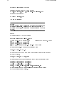
B.4 `perc.lsodes.in'
#--------------------------------------------------------# perc.lsodes.in
#
# Copyright (c) 1993. Don Maszle, Frederic Bois. All rights reserved.
#
#--------------------------------------------------------SimType (DefaultSim);
Integrate (Lsodes, 1e-4, 1e-6, 1);
#--------------------------------------------------------# The following experiment is for a simulation of one of Dr. Monster's
# exposure experiments described in "Kinetics of Tetracholoroethylene
# in Volunteers; Influence of Exposure Concentration and Work Load,"
# A.C. Monster, G. Boersma, and H. Steenweg,
# Int. Arch. Occup. Environ. Health, v42, 1989, pp303-309
#
# The paper documents measurements of levels of TCE in blood and
# exhaled air for a group of 6 subjects exposed to
# different concentrations of PERC in air.
#
# Inhalation is specified as a dose of magnitude InhMag for the
# given Exposure time.
#
# Inhalation is given in ppm
#--------------------------------------------------------Experiment {
InhMag = 72;
Period = 1e10;
Exposure = 240;
# ppm
# Only one dose
# 4 hour exposure
# measurements before end of exposure and at [5' 30'] 2hr 18 42 67 91 139 163
Print (C_exh_ug, 239.9 245 270 360 1320 2760 4260 5700 8580 10020 );
Print (C_ven, 239.9 360 1320 2760 4260 5700 8580 10020 );
}
END.
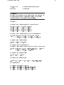
Appendix B: Examples
Vmax = sc_Vmax * exp (0.7 * log (LeanBodyWt));
} # End of model scaling
#--------------------------------------------------------# CalcOutputs
# The following outputs are only calculated just before values
# are saved. They are not calculated with each integration step.
#--------------------------------------------------------CalcOutputs {
# Fraction of TCE metabolized per day
Pct_metabolized = (InhMag ?
Qmet / (1440 * Flow_alv * InhMag * mg_per_l_per_PPM) :
0);
C_exh_ug
= C_exh * 1000; # milli to micrograms
} # End of output calculation
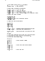
53
52
MCSim User' Manual
# Quantity metabolized in liver
dQmet_liv = Vmax * Q_liv / (Km + Q_liv);
dt (Q_liv) = Flow_liv * (C_art - Cout_liv) - dQmet_liv;
# Metabolite formation
dt (Qmet)
= dQmet_liv;
} # End of Dynamics
#--------------------------------------------------------# Scale
# Scale certain model parameters and resolve dependencies
# between parameters. Generally the scaling involves a
# change of units, or conversion from percentage to actual
# units.
#--------------------------------------------------------Scale {
# Volumes scaled to actual volumes
BodyWt = LeanBodyWt/(1 - Pct_M_fat);
V_fat
V_liv
V_wp
V_pp
=
=
=
=
Pct_M_fat * BodyWt/0.92;
# density of fat = 0.92 g/ml
Pct_LM_liv * LeanBodyWt;
Pct_LM_wp * LeanBodyWt;
0.9 * LeanBodyWt - V_liv - V_wp; # 10% bones
# Calculate Flow_alv from total pulmonary flow
Flow_alv = Flow_pul * 0.7;
# Calculate total blood flow from the alveolar ventilation rate and
# the V/P ratio.
Flow_tot = Flow_alv / Vent_Perf;
# Calculate actual blood flows from total flow and percent flows
Flow_fat
Flow_liv
Flow_pp
Flow_wp
=
=
=
=
Pct_Flow_fat * Flow_tot;
Pct_Flow_liv * Flow_tot;
Pct_Flow_pp * Flow_tot;
Flow_tot - Flow_fat - Flow_liv - Flow_pp;
# Vmax (mass/time) for Michaelis-Menten metabolism is scaled
# by multiplication of bdw^0.7
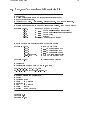
Appendix B: Examples
51
Flow_alv = 0;
# Alveolar ventilation rate
Vmax = 0;
# kg/minute
#--------------------------------------------------------# Dynamics
# Define the dynamics of the simulation. This section is
# calculated with each integration step. It includes
# specification of differential equations.
#--------------------------------------------------------Dynamics {
# Venous blood concentrations at the organ exit
Cout_fat
Cout_wp
Cout_pp
Cout_liv
=
=
=
=
Q_fat
Q_wp
Q_pp
Q_liv
/
/
/
/
(V_fat
(V_wp
(V_pp
(V_liv
*
*
*
*
PC_fat);
PC_wp);
PC_pp);
PC_liv);
# Sum of Flow * Concentration for all compartments
dQ_ven = Flow_fat * Cout_fat + Flow_wp * Cout_wp
+ Flow_pp * Cout_pp + Flow_liv * Cout_liv;
# Venous blood concentration
C_ven =
dQ_ven / Flow_tot;
# Arterial blood concentration
# Convert input given in ppm to mg/l to match other units
C_art = (Flow_alv * C_inh / PPM_per_mg_per_l +
(Flow_tot + Flow_alv / PC_art);
dQ_ven) /
# Alveolar air concentration
C_alv = C_art / PC_art;
# Exhaled air concentration
C_exh = 0.7 * C_alv + 0.3 * C_inh / PPM_per_mg_per_l;
# Differentials
dt
dt
dt
dt
(Q_exh)
(Q_fat)
(Q_wp)
(Q_pp)
=
=
=
=
Flow_alv
Flow_fat
Flow_wp
Flow_pp
*
*
*
*
C_alv;
(C_art - Cout_fat);
(C_art - Cout_wp);
(C_art - Cout_pp);
50
MCSim User' Manual
C_inh = PerDose (InhMag, Period, 0.0, Exposure);
LeanBodyWt = 55;
# lean body weight
# Percent mass of tissues with ranges shown
Pct_M_fat
Pct_LM_liv
Pct_LM_wp
Pct_LM_pp
=
=
=
=
.16;
.03;
.17;
.70;
#
#
#
#
% total body mass
liver, % of lean mass
well perfused tissue, % of lean mass
poorly perfused tissue, will be recomputed in scale
# Percent blood flows to tissues
Pct_Flow_fat
Pct_Flow_liv
Pct_Flow_wp
Pct_Flow_pp
=
=
=
=
.09;
.34;
.50; # will be recomputed in scale
.07;
# Tissue/blood partition coeficients
PC_fat
PC_liv
PC_wp
PC_pp
PC_art
=
=
=
=
=
144;
4.6;
8.7;
1.4;
12.0;
Flow_pul
= 8.0;
Vent_Perf = 1.14;
# Pulmonary ventilation rate (minute volume)
# ventilation over perfusion ratio
sc_Vmax = .0026;
# scaling coeficient of body weight for Vmax
Km = 1.0;
# The following parameters are calculated from the above values in
# the Scale section before the start of each simulation.
# They are left uninitialized here.
BodyWt = 0;
V_fat
V_liv
V_wp
V_pp
=
=
=
=
0;
0;
0;
0;
Flow_fat
Flow_liv
Flow_wp
Flow_pp
=
=
=
=
# Actual volume of tissues
0;
0;
0;
0;
Flow_tot = 0;
# Actual blood flows through tissues
# Total blood flow
Appendix B: Examples
49
B.3 `perc.model': A sample model description le
#--------------------------------------------------------# perc.model
# A four compartment model of Tetrachloroethylene (PERC)
# and total metabolites.
# Copyright (c) 1993. Don Maszle, Frederic Bois. All rights reserved.
#--------------------------------------------------------# States are quantities of PERC and metabolite formed, they can be output
States = {Q_fat,
Q_wp,
Q_pp,
Q_liv,
Q_exh,
Qmet};
# Quantity of PERC in the fat
#
...
in the well-perfused compartment
#
...
in the poorly-perfused compartment
#
...
in the liver
#
...
exhaled
# Quantity of metabolite formed
# Extra outputs are concentrations at various points
Outputs = {C_liv,
C_alv,
C_exh,
C_ven,
Pct_metabolized,
C_exh_ug};
#
#
#
#
#
#
mg/l in the liver
... in the alveolar air
... in the exhaled air
... in the venous blood
% of the dose metabolized
ug/l in the exhaled air
Inputs = {C_inh}
# Concentration inhaled
# Constants
# Conversions from/to ppm: 72 ppm = .488 mg/l
PPM_per_mg_per_l = 72.0 / 0.488;
mg_per_l_per_PPM = 1/PPM_per_mg_per_l;
#--------------------------------------------------------# Nominal values for parameters
# Units:
# Volumes: liter
# Vmax:
mg / minute
# Weights: kg
# Km:
mg / minute
# Time:
minute
# Flows:
liter / minute
#--------------------------------------------------------InhMag = 0.0;
Period = 0.0;
Exposure = 0.0;
48
MCSim User' Manual
SDw_ka = 0;
SDb_ke = 0;
SDw_ke = 0;
SDb_V = 0;
min_F = 0;
max_F = 0;
SD_C_central = 0;
SD_AUC
= 0;
CV_C_cen
= 0;
CV_AUC
= 0;
CV_C_cen_true = 0;
CV_AUC_true
= 0;
# Calculate Outputs
CalcOutputs {
# algebraic equation for C_central
C_central = (ka != ke ?
(exp(-ke * t) - exp(-ka * t)) *
F * ka * Dose / (V * (ka - ke))):
exp(-ka * t) * ka * t * F * Dose / V);
# algebraic equation for AUC
AUC = (ka != ke ?
((1 - exp(-ke * t)) / ke - (1 - exp(-ka * t)) / ka) * F * ka * Dose /
(V * (ka - ke))):
F * Dose * (1 - (1 + ka * t) * exp(-ka * t)) / (V * ke));
C_central = C_central + NormalRandom(0, C_central * CV_C_cen_true);
AUC
= AUC + NormalRandom(0, AUC * CV_AUC_true);
ln_C_central = (C_central > 0 ? log (C_central) : -100);
ln_AUC = (AUC > 0 ? log (AUC) : -100);
SD_C_computed = (C_central > 0 ? C_central * CV_C_cen : 1e-10);
SD_A_computed = (AUC > 0 ? AUC * CV_AUC : 1e-10);
} # End of output calculations
Appendix B: Examples
Appendix B Examples
You will nd here some examples of model description les and simulation iput les.
B.1 `linear.model'
# Linear Model with a random component
# y = A + B * time + N(0,SD_true)
# Setting SD_true to zero gives the deterministic version
#--------------------------------------------------------# Outputs
Outputs = {y};
# Model Parameters
A = 0;
B = 1;
SD_true = 0;
SD_esti = 0;
CalcOutputs { y = A + B * t + NormalRandom(0,SD_true); }
B.2 `1cpt.model': A sample model description le
# One Compartment Model
# First order input and output
#--------------------------------------------------------# Inputs
Inputs = {Dose};
# Outputs
Outputs = {C_central, AUC, ln_C_central, ln_AUC,
SD_C_computed, SD_A_computed};
# Model Parameters
ka = 1;
ke = 0.5;
F = 1;
V = 2;
# Statistical Parameters
SDb_ka = 0;
47
46
MCSim User' Manual
Appendix A: Using make
45
Appendix A Using make
is a utility that facilitates doing repetitive tasks like compilation. A `makefile' is a text
le that contains a description of what make should do and under what circumstances. For example
the compilation `Makefile' included with the MCSim distribution only compile a C-le if it has
changed since the last compilation. This means that when you change your model and create a new
`model.c' le using mod, only the `model.c' le needs to be compiled to recreate the simulation
engine.
Make
Before you run make for the rst time on a machine you must change some settings in the
makele to specify where your C compiler is on your le system, and some special settings for that
compiler. Refer to the documentation (or manual pages in Unix) for your compiler to do this.
In the makele le there are several variables dened which you may need to change. They are
described in the makele itself.
You run the make program by entering make or make -f Makefile at the prompt from the
directory where the program is that you want to compile.
44
MCSim User' Manual
Chapter 7: Common Pitfalls
43
7 Common Pitfalls
The following mistakes are particularly easy to make, and sometimes hard to notice, or understand at rst.
Putting a space before the end of line ; in the model denition le may causes strange error
messages.
Forgetting about type-related arithmetics in C: `1000/882' gives `1' since it is interpreted as
an integer division by the compiler. To get a oating-point (usual) division use `1000./882.'.
42
MCSim User' Manual
Park, S. K. and Miller, K. W. (1988). Random number generators: good ones are hard to nd.
Communications of the ACM 31:1192-1201.
Press, W. H., Flannery, B. P., Teukolsky, S. A. and Vetterling, W. T. (1989). Numerical Recipes
(2st ed.). Cambridge University Press, Cambridge.
Smith, A. F. M. (1991). Bayesian computational methods. Philosophical Transactions of the
Royal Society of London, Series A 337:369-386.
Smith, A. F. M. and Roberts, G. O. (1993). Bayesian computation via the Gibbs sampler and
related Markov chain Monte Carlo methods. Journal of the Royal Statistical Society Series B
55:3-23.
Vattulainen, I., Ala-Nissila, T. and Kankaala, K. (1994). Physical tests for random numbers in
simulations. Physical Review Letters 73:2513-2516.
Bibliographic References
41
Bibliographic References
Barry, T. M. (1996). Recommendations on the testing and use of pseudo-random number
generators used in Monte Carlo analysis for risk assessment. Risk Analysis 16:93-105.
Bernardo, J. M. and Smith, A. F. M. (1994). Bayesian Theory. Wiley, New York.
Bois, F. Y., Gelman, A., Jiang, J., Maszle, D., Zeise, L. and Alexeef, G. (1996). Population
toxicokinetics of tetrachloroethylene. Archives of Toxicology 70:347-355.
Bois, F. Y., Zeise, L. and Tozer, T. N. (1990). Precision and sensitivity analysis of pharmacokinetic models for cancer risk assessment: tetrachloroethylene in mice, rats and humans. Toxicology
and Applied Pharmacology 102:300-315.
Gear, C. W. (1971a). Algorithm 407 - DIFSUB for solution of ordinary dierential equations
[D2]. Communications of the ACM 14:185-190.
Gear, C. W. (1971b). The automatic integration of ordinary dierential equations. Communications of the ACM 14:176-179.
Gelman, A. (1992). Iterative and non-iterative simulation algorithms. Computing Science and
Statistics 24:433-438.
Gelman, A., Bois, F. Y. and Jiang, J. (1996). Physiological pharmacokinetic analysis using
population modeling and informative prior distributions. Journal of the American Statistical Association 91:1400-1412.
Gelman, A., Carlin, J. B., Stern, H. S. and Rubin, D. B. (1995). Bayesian Data Analysis.
Chapman & Hall, London.
Gelman, A. and Rubin, D. B. (1992). Inference from iterative simulation using multiple sequences (with discussion). Statistical Science 7:457-511.
Hammersley, J. M. and Handscomb, D. C. (1964). Monte Carlo Methods. Chapman and Hall,
London.
Manteufel, R. D. (1996). Variance-based importance analysis applied to a complex probabilistic
performance assessment. Risk Analysis 16:587-598.
40
MCSim User' Manual
The tab-delimited le can easily be imported into your favorite spreadsheet, graphic or statistical
package for further analysis.
6.7 Error Handling
If integration fails for an Experiment in DefaultSim simulations no output is generated for
that experiment, and the user is warned by an error message on the screen. In MonteCarlo or
SetPoints simulations, the corresponding simulation line is not printed, but the iteration number
is incremented. Finally, in MCMC simulations, the parameter for which the data likelihood was
computed is simply not updated (which implicitly forbids the uncomputable region of the parameter
space). In all cases an error message is given on the screen, or wherever the screen output has been
redirected.
Chapter 6: Specifying Simulations
39
An important concept to grasp here is that of "instance". In the code fragment given above,
the parameter A, dened at sub-level 1, is "cloned" as many times as there are sub-levels or
experiments enclosed in sub-level 1 (hence, it will be cloned twice in the example above, once for
each Experiment dened). In that way, the parameters distributions dened at one level in fact
apply to the next lower sub-level, or at the Experiment level. This convention saves a lot writing
and eort in the long run. For example, the uniform distribution assigned to A, at the top level,
applies to the sub-level 1. There is only one "clone" of A at sub-level 1 since only one sub-level is
included in the top level. In contrast, two normally-distributed "clones" of A will be dened and
sampled. The rst one will apply to experiment 1, and will be conditioned by the data of that
experiment only, and the other will apply to experiment 2. A total of three variables of "type" A
will be sampled and will be printed in the output le (coded so that the position in the hierarchy
is apparent): the "parent" A(1), a priori uniformly distributed, and two "dependents" A(1.1) and
A(1.2), a priori normally distributed around A(1).
6.6 Analyzing results
The output from Monte Carlo or SetPoints simulations is a tab-delimited text le with one
row for each run (i.e., parameter set) and one column for each parameter and output in the order
specied. Thus each line of the output le is in the following order:
<# of run> <parameters> <outputs for Exp 1> <outputs for Exp2> ...
The parameters are printed in the order they were sampled or set.
The rst line gives the column headers. A variable called name requested for output in an
experiment i at a time j is labeled name i.j.
The output of Markov chain Monte Carlo simulations is also a text le with one row for each
run. It displays a column of iteration labels, and one column for each parameter sampled. The last
three columns contain respectively, the sum of the logarithms of each parameter's density given
its parents' values (`LnPrior'), the logarithm of the data likelihood (`LnData'), and the sum of
the previous two values (`LnPosterior'). The rst line gives the column headers. On this line,
parameters names are tagged with a code identifying their position in the hierarchy dened by the
Level statements. For example, the second instance of a parameter called name placed at the st
level of the hierarchy is labeled name(2); the rst instance of the same parameter placed at the
second instance of the second level of the hierarchy is labeled name(2.1), etc.
38
MCSim User' Manual
specied via a PrintStep() specication (see Section 6.4.4 [PrintStep() specication], page 35),
since they are equally spaced. More generally, a Print() specication could have been used (see
Section 6.4.3 [Print() specication], page 34). The data values are given in a Data() statement.
6.5.1
Level
denition
Markov chain Monte Carlo simulations require the denition of a statistical model and the use
of the Level keyword. At least one level must be dened. A level section starts with the keyword
Level and is enclosed in curly braces. It can include any number of sub-levels or Experiments.
Experiments (where the data are specied) form the lowest level of the hierarchy (see Section 6.4.1
[Experiment denition], page 33. There must be one and only one top level and at most 10 sub-levels
in the hierarchy. This limit of 10 levels can be increased (up to 255) by changing MAX LEVELS
in the header le `sim.h' and recompiling.
A level can make modications to the sampling distribution of any model parameter. For
example:
Level { # this is the top level
Distrib(A, Uniform, 0, 1);
}
Level { # this is sub-level 1
Distrib(A, Normal, A, 1);
Experiment { ... } # experiment 1
Experiment { ... } # experiment 2
}
These distribution assignments apply to all sub-levels of the level where they take place. If
several assignments are given, their position within the level section is irrelevant (although a logical
order is recommended for clarity).
A level can also make modications to any model parameter that was dened in the global
section of the model description le. The syntax is the same, except that variables can only take
constant values. So, for example, in an experiment, the parameter A could be modied with:
A = 2.0;
This overrides any previously assigned values, even if randomly sampled, for the specied parameter. This assignment also applies to the sub-levels of the level where they take place.
Chapter 6: Specifying Simulations
37
We now need to write an input le specifying the distribution of y (i.e., the likelihood), and the
prior distributions of the various parameters. Here is what such a le could look like:
# --------------------------------------------------------------# Simulation input file for a linear regression
# --------------------------------------------------------------SimType (MCMC);
MCMC ("linear.MCMC.out", "", "", 50000, 0, 5, 40000, 63453.1961);
Level {
Distrib(Alpha,
Normal_v, 0, 10000);
Distrib(Beta,
Normal_v, 0, 10000);
Distrib(Sigma2, InvGamma, 0.01, 0.01);
Distrib(y, Normal_v, Prediction(y), Sigma2);
Experiment {
x_bar = 3.0;
PrintStep (y, 1, 5, 1);
Data
(y, 1, 3, 3, 3, 5);
}
} # end Level
End
# ---------------------------------------------------------------
The le begins the obvious SimType() (see Section 6.3.1 [SimType() specication], page 25)
and MCMC() (see Section 6.3.6 [MCMC() specication], page 30) keywords. The keyword Level
comes next. Level is used to specify the dependence between model parameters in a hierarchy.
There should be at least one Level in every MCMC input le, even for a non-hierarchical model
like the one above (actually, "non-hierarchical" models can be thought of has having only one level
of hierarchy). See below for further discussion of the Level keyword. You can also look at the
MCMC input les provided as examples with MCSim source code. The Distrib() statements
dene the parameter priors. Normal_v specications are used since we use variances instead of
standard deviations. The inverse-Gamma distribution is used for the variance component, since
the precision is supposed to be Gamma-distributed. The likelihood is the distribution of the data,
given the model: it is also specied by a Distrib() statement, valid for every y data point. Again,
note that the variable is not used. Instead the Prediction(y ) specication is used to signify
the linear model output. These distributions are in eect for every sub-level or every Experiment
included in the current level.
The "simulations" to perform, and the corresponding data values, are specied by the
Experiment section. Only one Experiment is needed here, but several could be specied. In
this section, the value of x is provided. The dierent values of x (time in our model) can be
36
MCSim User' Manual
is treated as "missing data" and ignored in likelihood calculations. The convention "-1" can be
changed by changing INPUT MISSING VALUE in the header le `mc.h' and recompiling.
6.5 Specifying a statistical model
Statistical models are dened in the simulation specication le, rather than in the model
denition le. It is necessary to dene a statistical model (with parameter dependencies, prior
distributions and likelihood) if you want to use MCMC sampling. MCMC sampling will then
give you in output a sample of parameters drawn from their joint posterior distribution. Take for
example the simple linear regression model:
yi = N (i; 2)
i = + (xi , x)
(1)
(2)
where the observed (x; y ) pairs are (1; 1), (2; 3), (3; 3), (4; 3) and (5; 5). The quantities and are given N (0; 10000) priors, and 1= 2 is given a Gamma(10,3; 10,3) prior. We want the posterior
distributions of , , and 2.
The rst thing to do is to dene a model to compute y as a function of x. Here is such a model
(quite similar to the one distributed with MCSim source code (see Section B.1 [linear.model],
page 47):
# --------------------------------------------# Model definition file for a linear model
# --------------------------------------------Outputs = {y};
# Model parameters
Alpha = 0;
Beta = 0;
Sigma2 = 1;
x_bar = 0;
CalcOutputs { y = Alpha + Beta * (t - x_bar); }
# ---------------------------------------------
The parameters' initialization values are arbitrary, and could be anything reasonable. They will
be changed or sampled through the input le. Note that 2 is not used in the model equations,
but still needs to be dened here in order to be part of the statistical model. On the other hand, is not dened, since we do not really need it. Finally x is replaced by the time, t, for convenience.
An alternative would be to dene an input `x' and use it instead of t.
Chapter 6: Specifying Simulations
35
Print(<identifier1>, <identifier2>, ..., <time1>, <time2>, ...);
The same output times are used for all the variables specied. The size of the time list is only
limited by the available memory. The limit of 10 variables names can be increased by changing
MAX PRINT VARS in the header le `sim.h' and recompiling. The number of Print() statements
you can used in a given Experiment section is only limited by the available memory.
6.4.4
PrintStep()
specication
The value of any model variable, input or parameter can be also output with PrintStep specications. They allow dense printing, suitable for smooth plots, for example. The arguments are the
name of only one variable, the rst output time, the last one, and a time increment:
PrintStep(<identifier>, <start-time>, <end-time>, <time-step>);
The nal time has to be superior to the initial time and the time step has to be less than the
time span between end and start. If the time step is not an exact divider of the time span the
last printing step is shorter and the last output time is still the end-time specied. The number
of outputs produced is only limited by the memory available at run time. You can use several
PrintStep() in a given Experiment section.
6.4.5
Data()
specication
Experimental observations of model variables, inputs, outputs, or parameters, can be specied
with the Data() command. Markov chain Monte Carlo sampling requires that you specify Data()
statements (see Section 6.3.6 [MCMC() specication], page 30; see Section 6.5.1 [Specifying a
statistical model], page 38). The data are then used internally to evaluate the likelihood function
for the model. The arguments are the name of the variable for which observations exist, and a list
of data values:
Data(<identifier>, <value1>, <value2>, ...);
This specication can only be used with a matching Print() or PrintStep() for the same variable (see Section 6.4.3 [Print() specication], page 34; see Section 6.4.4 [PrintStep() specication],
page 35). You must make sure that there are as many data values in the Data() specication
as output time requested in the corresponding Print() or PrintStep(). A data value of "-1"
34
MCSim User' Manual
This overrides any previously assigned values, even if randomly sampled, for the specied parameter.
Inputs can be redened with the input functions listed in the Mod reference section above (see
Chapter 5 [Dening Models], page 13). Input functions can reference other variables (eventually
random), as in:
Q_gav = PerExp(GavMag, 60, 0, RateConst);
The maximum number of experiments denable is 200. This can be changed by changing
MAX INSTANCES and MAX EXPERIMENTS in the header le `sim.h' and recompiling. Within
an experiment denition, or at the global level (if you want them to apply to all experiments), several
additional specications can also be used:
StartTime(),
Print(),
PrintStep(),
Data().
6.4.2
StartTime()
specication
The origin of time for a simulation, if it needs to be dened, is specied with the StartTime()
specication:
StartTime(<initial-time>);
If this specication is not given, a value of zero is used by default. The nal time is automatically
computed to match the largest output time specied in the Print() or PrintStep() statements (see
Section 6.4.3 [Print() specication], page 34; see Section 6.4.4 [PrintStep() specication], page 35).
6.4.3
Print()
specication
The value of any model variable, input, output or parameter can be requested for output with
Print() specications. Their arguments are a list of names of variables (at least one and up to 10),
and a list of increasing times at which to output their value:
Chapter 6: Specifying Simulations
33
If a null string is given for the output lename, the set points output will be written to the same
default output le used for Monte Carlo analyses, `simmc.out'.
The set points le name is required and must refer to an existing le containing the parameter
values to use. The rst line of the set points le is skipped and can contain column headers, for
example. Each of the other lines should contain an integer (e.g., the line number) followed by
values of the various parameters in the order indicated in the SetPoints() specication. If extra
elds are at the end of each line they are skipped. The rst integer eld is needed but not used
(this allows you to directly use Monte Carlo output les for additional SetPoints simulations).
The variable nRuns should be less or equal to the number of lines (minus one) in the set points
le. If a zero is given, all lines of the le are read. The format of the output le of set points
simulations is discussed below (see Section 6.6 [Analyzing results], page 39).
Following the SetPoints() specication, Distrib() statements can be given for parameters
not already in the list (see Section 6.3.5 [Distrib() specication], page 28). These parameters
will be sampled accordingly before to performing each simulation. The shape parameters of the
distribution specications can reference other parameters, including those of the list.
6.4 Specifying basic conditions to simulate
Any simulation le must dene at least one Experiment to simulate.
6.4.1
Experiment
denition
After global simulation specications, "experiments" must be included in the input le. They
dene simulation conditions and specify outputs. An "experiment" section starts with the keyword
Experiment and is enclosed in curly braces.
An "experiment" can make modications to any model variable or parameter that was dened
in the global section of the model description le. The syntax is the same, except that variables
or parameters can only take constant values. So, for example, in an experiment the body weight
could be modied with:
BodyWt = 83.2;
32
MCSim User' Manual
To recapitulate, the extended Distrib() syntax, for use with MCMC simulations is therefore:
Distrib(<identifier>, <iType>, [<shape parms>]);
where the rst two shape parameters can be Prediction(<identier>), or any model parameter or
numerals, and the last two shape parameters numerals only (this limitation will also be removed
in a future release).
If a statement like:
Distrib(Var, <iType>, Prediction(<Var>), Prediction(<Other_Var>), ...);
is used, the two variables Var and Other Var must have identical output times. It is then useful
to group them in the same Print() statement.
The other tool MCSim brings you to build a complete statistical model is the Level keyword.
The use of this keyword, is described below (see Section 6.5.1 [Specifying a statistical model],
page 38).
Finally, the format of the output le of MCMC simulations is discussed in a later section (see
Section 6.6 [Analyzing results], page 39).
6.3.7
SetPoints()
specication
To impose a series of set points (i.e., already tabulated values for the parameters), the global
section can include a SetPoints() specication. It allows you to perform additional simulations
with previously Monte Carlo sampled parameter values, eventually ltered. You can also generate
parameters values in a systematic fashion, over a grid for example, with another program, and use
them as input to MCSim. Importance sampling, latin hypercube sampling, grid sampling, can be
accommodated in this way.
This command species an output lename, the name of a text le containing the chosen parameter values, the number of simulations to perform and a list of model parameters to vary. It
has the following syntax:
SetPoints("<OutputFilename>", "<SetPointsFilename>", <nRuns>,
<identifier>, <identifier>, ...);
Chapter 6: Specifying Simulations
31
numbers, printing times, data values and the corresponding model predictions, computed using the
last parameter vector of the restart le. This is useful to quickly check the model t to the data.
If simTypeFlag is equal to 2, the entire restart le is used to compute the parameters' covariance
matrix. All parameters are then updated at once using a multivariate normal kernel as proposal
distribution of the Metropolis steps. This results in large improvement in speed. However, we
recommend that this option be used only when convergence is approximately obtained (therefore,
you should run MCMC simulations with simTypeFlag set to 0 rst, up to approximate convergence,
and then restart the chain with the ag at 2).
The integer printFrequency should be set to 1 if you want an output at each iteration, to 2 if you
want an output at every other iteration etc. itersToPrint is the number of nal iterations for which
output is required (e.g., 1000 will request output for the last 1000 iterations; to print all iterations
just set this parameter to the value of nRuns). Note that if no restart le is used, the rst iteration
is always printed, regardless of the value of itersToPrint. Finally, the seed of the pseudo-random
number generator can be any positive real number. Seeds between 1.0 and 2147483646.0 are used
as is, others are rescaled silently within those bounds.
To use the MCMC specication, you must dene a statistical model precising each parameter's
prior distribution, or conditional distribution (in the case of a hierarchical model), and the data
likelihood (i.e., the distribution of observation errors). These distributions must be enclosed in a
Level section and are specied with Distrib() statements (see Section 6.5.1 [Specifying a statistical model], page 38). In the context of MCMC sampling, MCSim provides an extension of
the Distrib() specication. First, the rst two shape parameters of distributions may depend on
other model parameters. For example:
Distrib(A, Normal, 0, 1);
Distrib(B, Normal, A, C);
The data distribution is given by a similar statement, which uses the specication Prediction() to
dierentiate data from their predicted counterparts. The Prediction() specication can be used
for the rst two shape parameters only (therefore, not for ranges, except in the case of uniform
or loguniform distributions). If Prediction() is used for the rst shape parameter, the variable
enclosed in parentheses must be the same as the variable whose distribution is described. There
should be one and only one distribution specied for a given type of data in the whole input le
(i.e., you cannot redene a likelihood; this limitation will hopefully be removed in a future release).
Note that only states and outputs can use Prediction() specications (but you can always dene
an output to be equal to a parameter or an input in your model le). For example:
Distrib(y, TruncNormal, Prediction(y), Prediction(z), -10, 10);
30
MCSim User' Manual
Distrib(B, Normal, A, 2);
6.3.6
MCMC()
specication
Markov chain Monte Carlo (MCMC) simulations, used in a Bayesian context, allow the user
to specify a statistical model (eventually hierarchical) and sample parameters from their joint
posterior distribution, given a prior distribution for each parameter, a set of data to simulate,
and corresponding likelihoods. Sampling from the posterior is not immediate: it requires the
simulation chain, which start by sampling purely from the prior, to reach equilibrium. Checking
that equilibrium is obtained is best achieved, in our opinion, by running multiple independent
chains. Hence these computations are very intensive. For a discussion of Markov chain Monte
Carlo and convergence issues you should consult the appropriate statistical literature (for example,
Bernardo and Smith, 1994; Gelman, 1992; Gelman et al., in press; Gelman et al., 1995; Gelman
and Rubin, 1992; Smith, 1991; Smith and Roberts, 1993) (see [Bibliographic References], page 41).
Technically, MCSim uses Metropolis-Hasting sampling and you do not need to worry about issues
of conjugacy or log-concavity of your prior or posterior distributions. Like simple Monte Carlo
simulations, MCMC simulations require the use of two specications, MCMC() and Distrib()
and of one special section denition: Level. The syntax for the MCMC() specication is:
MCMC("<OutputFilename>", "<RestartFilename>", "", <nRuns>,
<simTypeFlag>, <printFrequency>, <itersToPrint>, <RandomSeed>);
The output lename is a string eld and must be enclosed in quotes. If a null-string "" is given,
the default name `MCMC.default.out' will be used.
If a restart le name (enclosed in quotes) is given, the rst simulations will be read from that le
(which must be a text le). This allows you to continue a chain where you left it, since an MCMC
output le can be used as a restart le with no change. Note that the rst line of the le (which
typically contains column headers) is skipped. Also, the number of lines in the le must be less
than or equal to nRuns. The rst column of the le should be integers, and the following columns
(tab- or space-separated) should give the various parameters, in the same order as specied in the
list of Distrib() specications in the input le. The third eld is reserved for future use and
should just be a pair of empty quotes.
The integer nRuns gives the total number of runs to be performed, including the runs eventually
read in the restart le. The next eld, simTypeFlag should be either 0, 1, or 2. It should be set at
zero to start a chain of MCMC simulations. In that case, parameters are updated by Metropolis
steps, one at a time. If the value of simTypeFlag is set to 1 or 2, a restart le must also be
specied. In the case of 1, the output le will contain codes for the level sequence, experiment
Chapter 6: Specifying Simulations
29
Normal distribution (two reals numbers): mean and standard deviation, the latter being stricly
positive. The variant Normal_v takes the variance instead of the standard deviation as second
parameter.
Truncated normal distribution (four reals numbers): mean, standard deviation (stricly positive), minimum and maximum. The variant TruncNormal_v takes the variance instead of the
standard deviation as second parameter.
LogNormal distribution (two reals numbers): geometric mean (exponential of the mean in logspace) and geometric standard deviation (exponential, stricly superior to 1, of the standard
deviation in log-space). The variant LogNormal_v takes the variance (in log-space!) instead of
the standard deviation as second parameter.
Truncated Lognormal distribution (four reals numbers): geometric mean and geometric standard deviation (stricly superior to 1), minimum and maximum in natural space. For example:
Distrib(Var, TruncLogNormal, 1, 2.718, 0.01, 10)
samples Var such that ln(V ar) is a standardized normal variate { of mean ln(1) = 0 and
standard deviation ln(2:718) = 1 | while Var is truncated to fall between 0.01 to 10. The
variant TruncLogNormal_v takes the variance (in log-space!) instead of the standard deviation
as second parameter.
Beta distribution (at least two strictly positive real numbers): A and B. By default the Beta
distribution is dened over the interval [0;1]. If a range is given for the beta distribution, the
[0;1] interval is mapped onto the specied range.
Gamma distribution (two strictly positive real numbers): shape a and inverse scale b.
Inverse-gamma distribution (two strictly positive real numbers): shape a and scale b.
Chi-squared distribution (one strictly positive real number): n. This distribution is the same
as Gamma(n/2, 1/2).
Exponential distribution (one strictly positive real number): inverse-scale b.The density of this
distribution is equal to be,bx.
Binomial distribution (two strictly positive numbers, a real and an integer): p (in the interval
[0;1]), and N. If N is not input as an integer it will be rounded down during the simulations.
Poisson distribution (a strictly positive real): rate l.
Piecewise distribution (four reals): minimum, a, b, maximum. The distribution has the form
of a truncated triangle, with a plateau between a and b. If a = b, the distribution is the
triangular distribution.
The shape parameters of the above distribution specications can reference other parameters,
provided than distributions for these have already been dened. For example:
Distrib(A, Normal, 0, 1);
28
MCSim User' Manual
6.3.5
Distrib()
specication
This specication indicates which variable to sample, and its sampling distribution. One Distrib() specication must be included for each variable to sample. The specication le can include
any number of these commands at the global level, or within any Level section in the case of
Markov chain Monte Carlo sampling (see Section 6.5.1 [Specifying a statistical model], page 38).
The syntax is:
Distrib(<identifier>, <iType>, [<shape parms>]);
The iType eld species the sampling distribution to use and can be one of following:
Uniform,
LogUniform,
Normal,
Normal v,
LogNormal,
LogNormal v,
TruncNormal,
TruncNormal v,
TruncLogNormal,
TruncLogNormal v,
Beta,
Gamma,
InvGamma,
Chi2,
Exponential,
Binomial,
Poisson,
Piecewise.
The corresponding shape parameters (Bernardo and Smith, 1994; Gelman et al., 1995) (see
[Bibliographic References], page 41) are as follow:
Uniform and log-uniform distributions: minimum and maximum of the sampling range, real
numbers in natural space.
Chapter 6: Specifying Simulations
27
If the Integrate() specication is not used, the default integration method is Lsodes with
parameters 10,5, 10,7 and 1. We recommend using Lsodes, since is it highly accurate and ecient.
Euler can be used for special applications (e.g., in system dynamics) where a constant time step
and a simple algorithm are needed.
6.3.3
OutputFile()
specication
The OutputFile() specication allows you to specify a name for the output le of DefaultSim
simulations. If this specication is not given the name `sim.out' is used if none has been supplied
on the command-line or the initial dialog. The corresponding syntax is:
OutputFile("<OutputFilename>");
6.3.4
MonteCarlo()
specication
Monte Carlo simulations (Hammersley and Handscomb, 1964; Manteufel, 1996) (see [Bibliographic References], page 41) require the use of two specications, MonteCarlo() and Distrib(),
which must appear in the global section of the le, before the Experiment sections. Such Monte
Carlo specications are ignored if they appear in an Experiment specication.
The MonteCarlo specication gives general information required for the runs: the output le
name, the number of runs to perform, and a starting seed for the random number generator. Its
syntax is:
MonteCarlo("<OutputFilename>", <nRuns>, <RandomSeed>);
The output lename is a string eld and must be enclosed in quotes. If a null-string "" is given,
the default name `simmc.out' will be used. The seed of the pseudo-random number generator can
be any positive real number. Seeds between 1.0 and 2147483646.0 are used as is, others are rescaled
within those bounds (and a warning is issued). Here is an example of use:
MonteCarlo("percsimmc.out", 5, 9386.630);
The parameters' sampling distributions are specied by a list of Distrib specications, as
explained in the next section. The format of the output le of Monte Carlo simulations is discussed
later (see Section 6.6 [Analyzing results], page 39).
26
MCSim User' Manual
MCMC (previously Gibbs): Markov chain Monte Carlo simulations are performed to attain
the posterior distribution of the model's parameters, given their prior distributions | that
you specify | and data for which the likelihood function can be computed (see Section 6.3.6
[MCMC() specication], page 30),
SetPoints: the experiments are simulated using several lists of user-dened parameters values
in input (see Section 6.3.7 [SetPoints() specication], page 32).
If MonteCarlo, MCMC, or
needed (see below).
6.3.2
Integrate()
SetPoints
simulations are requested, additional specications are
specication
The integrator settings can be changed with the Integrate specication. Two integration routines
are provided: Lsodes (which originates from the SLAC Fortran library and is originally based on
Gear's routine) (Gear, 1971b; Gear, 1971a; Press et al., 1989) (see [Bibliographic References],
page 41) and Euler (Press et al., 1989).
The syntax for Lsodes is:
Integrate(Lsodes, <rtol>, <atol>, <method>);
Rtol is a scalar specifying the relative error tolerance for each integration step. Atol is a scalar
specifying the absolute error tolerance parameter. They apply to all integration variables (state
variables). The estimated local error in a state variable y(i) will be controlled so as to be roughly
less (in magnitude) than rtol jy (i)j + atol. Thus the local error test passes if, in each component,
either the absolute error is less than atol, or the relative error is less than rtol. Set rtol tozero for
pure absolute error control, and use atol to zero for pure relative error control. Caution: actual
(global) errors may exceed these local tolerances, so choose them conservatively. The method ag
should be 0 (zero) for non-sti dierential systems and 1 for sti systems. You should try both and
select the fastest for equal accuracy of output, unless insight from your system leads you to choose
a priori. In our experience, a good starting point for atol and rtol is about 10,6.
The syntax for Euler is:
Integrate(Euler, <time-step>, 0, 0);
time-step is a scalar specifying the constant time-step to be taken at each integration step. The
next two scalars are reserved for future use and should be set to zero.
Chapter 6: Specifying Simulations
25
# Input file (this is a comment)
SimType(MCMC);
<Global modifications and analysis specifications>
Level {
# Up to 10 levels of hierarchy
Experiment {
Specifications for first experiment
}
Experiment {
Specifications for second experiment
}
# Unlimited number of experiment specifications
} # end Level
End # Optional statement. Everything after this line is ignored
6.3 Global specications
The global section is used to give specications relevant to all experiments, for example specication of the type of analysis, how the integrator should work, parameter modications to be used
for all experiments, etc.
Both the global section and each experiment section can contain modications to dened model
variables. At the beginning of a simulation, all model parameters are initialized to the nominal
values specied in the model description le. Next, modications given in the global section are
applied, and nally any modications for the current experiment are applied.
6.3.1
SimType()
specication
The type of analysis performed is specied using the SimType() specication. Example:
SimType(MonteCarlo);
The following keywords can be used:
DefaultSim: the list of specied experiments is simulated,
MonteCarlo: the specied experiments are simulated several times with random input parameters (see Section 6.3.4 [MonteCarlo() specication], page 27),
24
MCSim User' Manual
6.2 Syntax of the simulation denition le
The le starts with a global declaration section followed by a number of Experiment (i.e.,
simulation) denitions (see Section 6.4.1 [Experiment denition], page 33), eventually enclosed in
a Level denition if Markov chain Monte Carlo simulations are to be performed (see Section 6.5.1
[Specifying a statistical model], page 38). Each Experiment denes simulation conditions, from an
initial time (or whatever your dependent variable represents) to a nal time. The initial values of
model state variables, parameter values, input variables, and which outputs are to print at which
times can all be changed in a given Experiment.
The general syntax of the le is the same as that of mod with two dierences:
Variables can only be assigned constant values.
Input variables' assignments can use any input function (including the NDoses() function) or
constant values.
Expressions are not allowed (unlike in the model denition le where they can be used). Similarly, structural change to the model, for instance, addition of a state, input, output or parameter,
cannot be done here and must be done in the model description le. The simulation specication
le is read until its end is reached, or until an End command is reached.
The general layout of the le is:
# Input file (this a comment)
<Global modifications and analysis specifications>
Experiment {
<Specifications for first experiment>
}
Experiment {
<Specifications for second experiment>
}
# Unlimited number of experiment specifications
End # Optional End statement. Everything after this line is ignored
For Markov chain Monte Carlo simulations (see Section 6.3.6 [MCMC() specication], page 30),
the general layout of the le includes Level denitions:
Chapter 6: Specifying Simulations
23
6 Specifying Simulations
After having your model dened and processed by mod, and the resulting `model.c' le compiled
with the MCSim routines, you are ready to run simulations. For this you need to write a simulation
le.
An example le `perc.lsodes.in', which works with the perchloroethylene model, appears in
Appendix (see Section B.4 [perc.lsodes.in], page 54).
6.1 Using the compiled program
The simulation environment MCSim provides several types of simulations for the models you
create. Simulations are specied in a text le of format similar to that of the model description
le.
In Unix the command-line syntax for the MCSim program is:
mcsim [input-file [output-file]]
where the brackets indicate optional arguments. This assume that you have not renamed the
executable le; If you have, substitute the name of your executable. If no input and output le
names are specied, the program will prompt you for them. If already one le name is given
on the command-line, the program will assume it species the input le and will prompt you for
the output le name. You must provide an input le name. If you just hit the return key when
prompted for the output name, the program will use the name you have specied in the input le,
if any, or a default name. When the program starts up, it announces which model description le it
was created with. The input le describes the simulations to perform and species which outputs
should be printed out (see Section 6.2 [Syntax of simulation les], page 24).
On the Macintosh you double-click the `MCSim' icon and enter the name of your simulation
denition le at the rst prompt and then the name of the output le (or just hit return if you
want the default or the name you have specied in the input le to be used).
22
MCSim User' Manual
Chapter 5: Dening Models
21
5.2.9 Note about models
MCSim can easily deal with algebraic models. You do not need to dene state variables or a
Dynamics section for such models. Simply use input and output variables and paramaters. The
model can be specied in the CalcOutputs section. You can use the time t if that is natural for
your model. If you do not use t in your model, you will still need to specify "output times" in
Print() or PrintStep() statements to obtain outputs: you can use an arbitrary time, such as
1. If you do not use t you will also need do dene an Experiment (see Section 6.4.1 [Experiment
denition], page 33) for each combination of values for the "independent" variables of your model.
This may be clumsy if many values are to be used. In that case, you may want to use the variable
t to represent something else than time.
Ordinary dierential models, with algebraic components, can be setup easily with MCSim. Use
state variables and specify a Dynamics section. Time, t is the integration variable, but here again,
t can be used to represent anything you want. We are not aware of cases in which MCSim has
been used for partial dierential equations. Some problems might be solved by implementing
rudimentary line methods...
You can use MCSim for discrete-time dynamic models (or dierence models). It's a bit tricky.
Assignments in CalcOutput are volatile (not memorized), so the model equations have to be in
Dynamics. But the model variables should still be declared as outputs, because they should not be
updated by integration. However, you need at least a true state in the Dynamics section, so you
should declare a dummy one (and give it a constant derivative of value zero). You also want the
calls to Dynamics to be precisely scheduled, so it is best to use the Euler integration routine (see
Section 6.3.2 [Integrate() specication], page 26) which uses a constant step. Since Euler may call
repeatedly Dynamics at any given time, you want to guard against untimely updating... Altogether,
we recommend that you examine the sample les `discrete.model' and `discrete.in' provided
with the source code for MCSim.
20
MCSim User' Manual
Only variables that have been declared with the keyword Outputs can be changed in this section.
Assignments to other types of variables cause an error message like the following to be issued:
Error: line 56: 'Qb_fat' used in invalid context.
Only outputs can be defined in CalcOutputs{} section.
Any reference to an input or state variable will use the last calculated (current) value of the
input. The dt() operator can appear in the right-hand side of equations, and it refers to values
of the derivative as calculated at the last time step (see Section 5.2.5 [Dynamics specications],
page 18). Like in the Dynamics section, the integration variable can be accessed if referred to as t,
as in:
Qx_out = DQx * t;
5.2.8 Comments on style
For your model le to be readable and understandable, it is useful to use a consistent style
of notation. The example le `perc.model' follows such a consistent notation (see Section B.3
[perc.model], page 49). For example we suggest that:
All variable names begin with a capital letter followed by meaningful lower case subscripts.
Where two subscripts are necessary, they can be separated by an underscore, such as in
`Qb_fat'.
Where there is only one subscript an underscore can still be used to increase readability as in
`Q_fat'.
Where two words are used in combination to name one item, they can be separated visually
by capitalizing each word, as in `BodyWt'.
These conventions are suggestions only. The key to have a consistent notation that makes sense
to you. Consistency is one of the best ways to:
1. Increase readability, both for others and for yourself. If you have to suspend work for a month
or two and then come back to it, the last thing you want is to have to decipher your own le.
2. Decrease the likelihood of mistakes. If all of the equations are coded with a consistent, logical
convention, mistakes stand out more readily.
Chapter 5: Dening Models
19
dt(Qm_in) = Qmetabolized - dt(Qm_out);
The integration variable (e.g., time) can be accessed if referred to as t, as in:
dt(Qm_in) = Qmetabolized - t;
Output variables can also be made a function of t in the Dynamics section.
Note that while state variables, input variables and model parameters can indeed be used on the
right-hand side of equations, they cannot be assigned values in the Dynamics section. If you need
a parameter to change with time, declare it as output variable in the global section. Assignments
to inputs or parameters in this section causes an error message like the following to be issued:
Error: line 48: 'YourParm' used in invalid context.
Parameters cannot be defined in Dynamics{} section.
5.2.6 Parameter scaling
The parameter scaling section begins with the keyword Scale and is enclosed in curly braces. The
equations given in this section will dene a function that will be called by the simulation program
at the beginning of each simulation of an Experiment (see Section 6.4.1 [Experiment denition],
page 33). They can therefore be used for initialization of the simulations.
All model variables and parameters can be changed in this section. Modications to state
variables aect initial values only. Modifying an input is not allowed and state variables can only
appear at the left hand side of equations.
The dt() operator (see Section 5.2.5 [Dynamics specications], page 18) cannot be used in this
section, since derivatives have not yet been computed when the scaling function is called.
5.2.7 Output calculations
The output calculation section begins with the keyword CalcOutputs and is enclosed in curly
braces. The equations given in this section will be called by the simulation program at each output
time specied by a Print() or PrintStep() statement (see Section 6.4.3 [Print() specication],
page 34, and see Section 6.4.4 [PrintStep() specication], page 35). In this way, the output scaling
is done eciently, only when values are to be saved, and not at each integration step.
18
MCSim User' Manual
Input functions can be combined to give a lot of exibility (e.g., an input can be sum of some
others). Separate inputs can be declared in the global section of the model denition le and
combined in the Dynamics and CalcOutputs sections. The only limitation is that for each input
function used, a separate input must be dened in the model, even though this function may not
be a real element of the model.
5.2.5 Dynamics specications
The dynamics specication section begins with the keyword Dynamics and is enclosed in curly
braces. The equations given in this section will be called by the integrator at each integration step.
Additional variables to those declared in the global section may be used for any calculations
within the section. They will be declared as local temporary variables. (Note, for example, the use
of `Cout_fat' and `Cout_wp' in the `perc.model' sample le). Local variables are not accessible
from the simulation program, or from other sections of the model denition le, so don't try to
output them.
Each state variable declared in the global section must have one corresponding state equation
in the Dynamics section. If a state equation is missing, mod issues an error message such as:
Error: State variable 'Q_foo' has no dynamics.
If one or more dierential equations are missing, no program le will be created. Most error
messages are self-explanatory. Where appropriate, they also show a line number in the input le
where the error occurred. Beware, however, of cascades of errors generated as a consequence of a
rst one; so don't panic: start by xing the rst one and rerun mod.
The derivative of a state variable is dened using the dt() operator, as shown here:
dt(state-variable) '=' constant-value-or-expression ';'
The right-hand side can be any valid C expression, including standard math library calls and
the special functions mentioned above (see Section 5.2.3 [Special functions], page 16). Note, however, that no syntactic check is performed on the library function calls. Their correctness is your
responsibility.
The dt() operator can also be used in the right-hand side of equations in the dynamics section
to refer to the value of a derivative at that point in the calculations. For example:
Chapter 5: Dening Models
17
5.2.4 Input functions
They can be used in a special assignments, valid only for input variables. Inputs can be initialized
as a constant or expression, or assigned one of the following input functions:
PerDose() species a periodic input of constant magnitude. The input begins at initial-time
in the period and lasts for exposure-time time units. Syntax:
PerDose(<magnitude>, <period>, <initial-time>, <exposure-time>);
PerExp() species a periodic exponential input. At time initial-time in the period the input
rises instantaneously to magnitude and begins to decay exponentially with the constant decayconstant. The input is turned o once the magnitude reaches a negligible fraction (10,6) of
its original value. Syntax:
PerExp(<magnitude>, <period>, <initial-time>, <decay-constant>);
NDoses() species a number of stepwise inputs of variable magnitude and their starting times.
The rst argument, n, is the number of input steps and start times. Next come a list of
magnitudes and a list of initial times. Each list is comma-separated. The duration of input
step is computed automatically by dierence between the specied times. Currently this
function can only be used in the simulation description le, and not in the model description
le (which simply implies that you cannot use it as a default). Syntax:
NDoses(<n>, <list-of-magnitudes>, <list-of-initial-times>);
Spikes() species a number of instantaneous inputs of variable magnitude and their exact times
of occurence. The rst argument, n, is the number of inputs and input times. Next come a
list of magnitudes and a list of times. Each list is comma-separated. Currently this function
can only be used in the simulation description le, and not in the model description le (which
simply implies that you cannot use it as a default). Syntax:
Spikes(<n>, <list-of-magnitudes>, <list-of-times>);
The arguments of input functions can either be constants or variables. As an example, if `GavMag'
and `RateConst' are dened model parameters, then the input variable `Q_gav' can be dened as:
Q_gav = PerExp(GavMag, 60, 0, RateConst);
In this way the parameters of input functions can, for example, be assigned statistical distributions in Monte Carlo simulations (see Section 6.3.5 [Distrib() specication], page 28).
Variable dependencies are resolved before the simulation is started. For each of the periodic
functions, a single exposure beginning at time initial-time can be specied by giving an eectively
innite period, e.g. 1010. The rst period starts at the initial time of the simulation. Magnitudes
change exactly at the times given.
16
MCSim User' Manual
If a global state, input, or output variable is not given an initial value, it will default to zero.
Initial values are reset to their specied value by the simulation program at the start of each
simulation of an Experiment (see Section 6.4.1 [Experiment denition], page 33).
All the model parameters you want to be able to change through simulation les should be
declared global. Parameters must be given nominal values, following the assignment rules given
above. For example:
BodyWt = 0.38 + sqrt(0.01); # (kg) Weight of the rat
All parameters and variables are computed in double precision oating-point numbers. Initialization values should not be such as to cause computation errors in the model equations; this is
likely to cause program crashes (so, for example, do not assign a default value of zero to a parameter
appearing alone in a denominator). Note that the order of global declarations matters within the
global section itself (i.e., parameters and variables should be dened and initialized before being
used in assignments of others), but not with respect to other blocks. A parameter dened at the
end of the description le can be used in the dynamics section which may appear at the beginning
of the le. Still, such an inverse order should be avoided. For this reason, the format above, where
global declarations come rst, is strongly suggested to avoid confusing results. Note again that the
name IFN, in capital letters, is reserved by the program and should not be used as parameter or
variable name. Finally, if a parameter is dened several times, only the rst denition is taken into
account.
5.2.3 Special functions
The following special functions (whoe name is case-sensitive) are available to the user for assignment of parameters and variables in the model denition le:
CDFNormal(x): the normal cumulative density function;
erfc(x): the error function;
lnDFNormal(x, mean, sd): the natural logarithm of the normal density function;
lnGamma(x): the natural logarithm of the gamma function;
UniformRandom(min, max): returns a uniformly distributed random variable, sampled between min and max. The algorithm used is that of Park and Miller (Barry, 1996; Park and
Miller, 1988; Vattulainen et al., 1994) (see [Bibliographic References], page 41). A default
random generator seed (314159265.3589793) is used;
NormalRandom(mean, sd): returns a normally distributed random variable. The default
random generator seed is used.
Chapter 5: Dening Models
15
erators allowed are the equality operator ==, and non-equality operators !=, <, >, <>, <= and
>=.
5.2.2 Global parameter declarations
Commands not specied within the delimiting braces of another section are considered to be
global declarations. In the global section, you rst declare the states, inputs, and outputs variables.
There should be at least one state or output variable in your model.
States are variables for which a rst-order dierential equation is dened (higher orders or
partial dierential equations are not allowed).
Inputs are variables independent of the others variables, but eventually varying with time (for
example an exposure concentration to a chemical).
Outputs are dependent model variables (obtainable at any time as analytical functions of the
states, inputs or parameters) that do not have dynamics.
The format for declaring each of these variables is the same, and consists of the keyword States,
Inputs or Outputs followed by a list of the variable names enclosed in curly braces as shown here:
States =
{Qb_fat, # Benzene in the fat
Qb_bm,
# ...
in the bone marrow
Qb_liv}; # ...
in the liver and others
Inputs =
{Q_gav,
C_inh};
Outputs =
{Cb_exp, # Concentration in expired air
Cb_ven}; # ...
in venous blood
# Gavage dose
# Inhalation concentration
After being dened, states, inputs and outputs can then be given initial values (constants or expressions). Note that inputs can also be assigned input functions, described below. Some examples
of initialization are shown here:
Qb_fat = 0.1; # Default initial value for state variable Qb_fat
# Gavage input assigned a periodic exponential input function
Q_gav = PerExp(1, 60, 0, 1); # Magnitude of 1.0,
# period of 60 time units,
# T0 in period is 0,
# Rate constant is 1.0
14
MCSim User' Manual
<Global parameter specifications>
Dynamics {
<Equations for calculating the dynamics, or state derivatives>
}
Scale {
<Equations for scaling model parameters>
}
CalcOutputs {
<Equations for scaling the outputs>
}
where Dynamics, Scale and CalcOutputs are keywords and, if used, must appear as shown, followed
by the curly braces which delimit the section. At least one of the sections Dynamics or CalcOutputs
should be dened. Dynamics must be used if the model includes dierential equations.
5.2.1 General syntax
The general syntax of the le is as follows:
Comments begin with a pound sign (#) and continue to the end of the line.
Blank lines are allowed and ignored.
All commands can span several lines and are terminated by a semi-colon (;). There should be
no blank space before the semi-colon.
Variable assignments have the following syntax:
var-name '=' constant-value-or-expression ';'
where var-name is any valid C identier, starting with a letter or underscore (_) and followed
by any number of alpha-numeric characters or underscores, up to a maximum of 80. Variable
names are case sensitive. Note that the name IFN, in capital letters, is reserved by the program
and should not be used as parameter or variable name. The equal sign is needed. The
right-hand side expression can be a valid C mathematical expression including already dened
variables and ANSI C mathematical functions. Additional functions, called special functions,
can be used, which take variable names, constant values or expressions as parameters. Special
functions are detailed below (see Section 5.2.3 [Special functions], page 16). Finally, there
should be no space before the terminating semi-colon.
Colon conditional assignments can also be used. Syntax:
var-name '=' (<condition> ? <value-if-true> : <value-if-false>);
For example:
Adj_Parm = (Input > 0.0 ? Parm * Adjust : Parm);
In this example, if `Input' is greater than 0, the parameter `Adj_Parm' is computed as the
product of `Parm' by `Adjust'; otherwise `Adj_Parm' is equal to `Parm'. The comparison op-
Chapter 5: Dening Models
13
5 Dening Models
Three examples of model simulation les: `linear.model', `1cpt.model' and `perc.model'
are included with the program les and appears in Appendix of this manual (see Appendix B
[Examples], page 47).
5.1 Using Mod to process model description les
The mod program is a stand-alone facility. It takes a model description le in the "user-friendly"
format described below and creates a C language le `model.c' which you will compile and link
to the simulation program. Mod allows the user to dene equations for the model, assign default
values to parameters or default initial values to model variables, and dene scaling functions for
both the input parameters and the outputs variables. Mod lets the user create and modify models
without having to maintain C code.
In Unix, the command line syntax for the mod program is:
mod [input-file [output-file]]
where the brackets indicate that the input and output lenames are optional. If the input lename
is not specied, the program will prompt for both. If only the input lename is specied, the output
is written by default to the le `model.c'. Unless you feel like doing some makele programming,
we recommend using this default since the makele for MCSim assumes the C language model le
to have this name. You have to have prepared an input le containing a description of the model
following the syntax described in the following (see Section 5.2 [Syntax of mod les], page 13).
On the Macintosh you double-click the `Mod' icon and enter the name of the model denition
le at the prompt (on the Macintosh, names can include space characters).
5.2 Syntax of the model description le
The model description le is a text (ASCII) le that consists of several sections, including global
declarations, dynamics specications (eventually with derivative calculations), model scaling, and
output computations:
# Model description file (this is a comment)
12
MCSim User' Manual
To start mod under Unix just type mod perc.model. On a Macintosh, double click the `Mod'
icon; Mod prompts you for the name of your model denition le; Type `perc.model'. After a few
seconds, with no error messages if the model denition is syntactically correct, Mod announces that
the `model.c' le has been generated. On a Macintosh you need to hit the return key to exit Mod.
The next step is to compile and link together the various C les that will constitute the simulation
program for your particular model. Note that each time you want to change an equation in your
model you will have to change the model denition le and repeat the steps above. However,
changing just parameter values or state initial values does not require recompilation since that can
be done through simulation specication les.
Under Unix, the simplest is to use the make utility. Just type make and compilation will be
done automatically (see Appendix A [Using make], page 45). An executable `mcsim' is created.
You can rename it to better describe the fact that it is model specic: rename it `mcsim_perc',
for example.
On a Macintosh, or PC, the best is to use a Think C project or a similar programming
environment. You should rst use the command make or its equivalent to compile the modied
`model.c' le and other C les. Then create an application (you should give it a name specic
to the model you are developing, e.g., `MCSim Perc'). Refer to your compiler manual for details
on how to use your programming environment. Your executable `MCSim Perc' program is now
ready to perform simulations.
To start your MCSim program just type mcsim_perc (if you gave it that name) under Unix, or
double click the `MCSim Perc' or whatever name you specied icon on your Macintosh. After an
introductory banner (telling in particular which model le the program has been compiled with),
you are prompted for an input le name: type perc.lsodes.in (see Section B.4 [perc.lsodes.in],
page 54, to see this le now). The program then prompts you for the output le name: type
perc.lsodes.out. After a few seconds or less (depending on your machine) the program announces
that it has nished and that the output le is `perc.lsodes.out' (on a Macintosh you should hit
the return key to exit the program completely). You can open the output le with any text editor
or word processor, you can edit it for input in graphic programs etc.
Several other models and simulation specication les are provided with the package as examples
(they are in the `sim' directory. Try them and observe the output you obtain. You can then start
programming you own models and doing simulations. The next sections of this manual reference
the syntax for model denition and simulation specications.
Chapter 4: Working Through an Example
11
4 Working Through an Example
Pharmacokinetics models describe the transport and transformation of chemical compounds in
the body. These models often include nonlinear rst-order dierential equations. The following
example is taken from our own work on the kinetics of tetrachloroethylene (a solvent) in the human
body (Bois et al., 1996; Bois et al., 1990) (see [Bibliographic References], page 41). Go to the `sim'
directory (under Unix) or to the `Development' folder (on a Macintosh). Open the le `perc.model'
with any text editor (e.g., emacs or vi under Unix). This le is distributed as an example of a
model denition le (see Section B.3 [perc.model], page 49). You can use it as a template for your
own model, but you should leave it unchanged for now. Notice that it denes:
state variables for the model (for which dierentials are dened), for example:
States = {Q_fat,
Q_wp,
Q_pp,
Q_liv,
Q_exh,
Qmet}
# Quantity of PERC in the fat
#
...
in the well-perfused compartment
#
...
in the poorly-perfused compartment
#
...
in the liver
#
...
exhaled
# Quantity of metabolite formed
output variables (obtainable at any time as analytical functions of the states, inputs and
parameters), for example:
Outputs = {C_liv,
C_alv,
C_exh,
C_ven,
Pct_metabolized,
C_exh_ug}
#
#
#
#
#
#
mg/l in the liver
... in the alveolar air
... in the exhaled air
... in the venous blood
% of the dose metabolized
ug/l in the exhaled air
input variables (independent of the others variables, and eventually varying with time), for
example:
Inputs = {C_inh} # Concentration inhaled
model parameters (independent of time), such as:
LeanBodyWt = 55; # lean body weight
system's dynamics (dierential or algebraic equations dening the model per se),
parameters' scaling (the parameters used in the equations can be made functions of other
parameters: for example volumes can be computed from masses and densities),
equations to compute the output variables.
This model denition le as a simple syntax, easy to master. It needs to be turned into a C
program le before compilation and linking to the other routines (integration, le management etc.)
of MCSim. You will use mod for that. First, quit the editor and return to the operating system.
10
MCSim User' Manual
of this manual (see Chapter 4 [Working Through an Example], page 11, which walk you through
an example of model building and running.
The makele `Test_mcsim' can be used to test whether the program output on your Unix
machine is the same as the one on our machines. Just type: make; make -f Test_mcsim when in
your `sim' directory. All input les will be run and their output compared to the corresponding
output les. You will need to have the `mod' program already compiled and inside the `sim' directory,
or on the command path. In case of dierences, don't panic: check the actual dierences between
the culprit output le and the le `sim.out' produced by the makele. Small dierences may occur
from dierent machine precision. This can happen for random numbers, in which case the Markov
chain simulations (MCMC) can diverge greatly after a while.
Chapter 3: Installation
9
3 Installation
3.1 System requirements
MCSim is written in ANSI-standard C language. We are distributing the source code and you
should be able to compile it for any system, provided you have an ANSI C compiler. On a Unix
system we recommend that you install the GNU gcc compiler (freeware) and the make utility
(which is in fact standard on most systems). For PC-type computers we recommend the Unix
operating system Linux. For the Macintosh, you can use version 8.0 (or higher) of Symantecs
Think C compiler, although other compilers should work.
3.2 Distribution
MCSim source code is available on Internet through `ftp://sparky.berkeley.edu/pub/mcsim',
`http://sparky.berkeley.edu/users/fbois/', and `http://www.gnu.ai.mit.edu/home.html'.
3.3 Machine-Specic Installation
To install on a given machine, download (in binary mode) the distributed archive le to your
machine.directory. Move it to an empty directory of any name. Decompress the archive with
GNU gunzip (gunzip <archive-name.gz>). Untar the decompressed archive with tar (tar xf
<archive-name>; do man tar for further help). On Macintosh machines the programme "Stut
Expander" should be able to both uncompress and untar the archive. This decompression will
create two directories: `mod' and `sim'.
Move to the `mod' directory. Under Unix, compile the mod program using the `Makefile' in that
directory (the command make should just do that). Under other operating systems, refer to the
documentation of your compiler to create an executable `mod' le from the source code provided in
the `mod' directory. Move the executable `mod' program you just created to the `sim' directory.
You are then ready to use MCSim. This requires creating a model denition le, processing it
with the mod program, and compiling the resulting `model.c' le with all the other C les in the
`sim' directory. You can then run simulations les. We recommend that you go to the next section
8
MCSim User' Manual
2.2 Types of simulations
Four types of simulations are available:
A DefaultSim simulation will simply solve (eventually integrate) the equations you specied,
using the default parameter values and possible overridings imposed in a simulation specication le. User-requested outputs are sent to an output le (see Section 6.3.1 [SimType()
specication], page 25).
A MonteCarlo simulation will perform repeated (stochastic) simulations across a randomly
sampled region of the model parameter space (see Section 6.3.4 [MonteCarlo() specication],
page 27).
A MCMC simulation performs a series of simulations along a Markov chain in the model
parameter space (see Section 6.3.6 [MCMC() specication], page 30). These are Monte Carlo
simulations in which the choice of a new parameter value is inuenced by the current value.
They can be used to obtain the Bayesian posterior distribution of the model parameters,
given their prior distributions (that you specify) and data for which a likelihood function can
be computed. The program handles hierarchical (random eect) statistical models, such as
population pharmacokinetic models (see Section 6.5.1 [Specifying a statistical model], page 38).
A SetPoints simulation solves the model for a series of specied parameter sets, listed in a
separate ASCII le (see Section 6.3.7 [SetPoints() specication], page 32). You can create these
parameter sets yourself or use the output of a previous Monte Carlo or MCMC simulation.
2.3 Major changes introduced with version 4.2.0
A new input function, Spikes() is available. It simulates instantaneous inputs (see Section 5.2.4
[Input functions], page 17).
Six new distributions are available for Monte Carlo simulations: InvGamma (inverse-gamma),
Piecewise, Normal v, LogNormal v, TruncNormal v, TruncLogNormal v (see Section 6.3.5
[Distrib() specication], page 28).
In Monte Carlo simulations, shape parameters of Distrib() statements can now reference
other sampled parameters (see Section 6.3.4 [MonteCarlo() specication], page 27).
A simTypeFlag option, in the MCMC() specication, allows the printing of times, data and
predictions for easy checking of the model t. It can also be set to switch MCMC sampling
from component by component sampling to vector sampling (see Section 6.3.6 [MCMC() specication], page 30).
Chapter 2: Overview
7
2 Overview
MCSim consists of two pieces, a model generator and a simulation engine. The model generator,
mod, was created to facilitate the model maintenance and simulation denition, while keeping
execution time fast. Other programs have been created to the same end, the Matlab family of
graphical interactive programs being some of the more general and easy to use. Still, many available
tools are not optimal for performing time and computer intensive Monte Carlo analyses. MCSim
was created specically to this end: to perform Monte Carlo analyses in a highly optimized, and
easy to maintain environment.
2.1 General procedure
Model building and simulation proceeds in four stages:
1. You create with any text editor a model description le. The reference section on mod, later
in this manual gives you the syntax to use (see Chapter 5 [Dening Models], page 13). This
syntax allows you to describe the model variables, parameters, equations, inputs and outputs
in a C-like fashion without having you to actually know how to write a C program.
2. You instruct the model generator, mod, to preprocess your model description le. Mod creates
a C le, called `model.c'.
3. You compile and link the newly created `model.c' le together with the other C program les.
MCSim C code is standard, so you should be able to compile it with any standard C compiler,
for example GNU gcc. After compiling and linking, an executable simulation program `mcsim'
is created, specic of the particular model you have designed. These preprocessing and compilation steps may seem clumsy but they produce the most ecient code for your particular
machine.
4. You design any number of simulation specication les and run them with the mcsim program.
The simulation specication les describe the kind of simulation to run (simple simulations,
Monte Carlo etc.), various settings for the integration algorithm if needed, and a description of
one or several experimental conditions or observations to simulate (see Chapter 6 [Specifying
Simulations], page 23). The simulation output is written to standard ASCII les.
Little or no knowledge of computer programming is required, unless you want to tailor the
program to special needs, beyond what is described in this manual (in which case you should
contact us). You need, however, some familiarity with program compilation under your operating
system (see Section 3.3 [System requirements], page 9). The software manual for your compiler
should be able to help you.
6
MCSim User' Manual
9. The Free Software Foundation may publish revised and/or new versions of the General Public
License from time to time. Such new versions will be similar in spirit to the present version, but
may dier in detail to address new problems or concerns.
Each version is given a distinguishing version number. If the Program species a version number
of this License which applies to it and "any later version", you have the option of following the
terms and conditions either of that version or of any later version published by the Free Software
Foundation. If the Program does not specify a version number of this License, you may choose any
version ever published by the Free Software Foundation.
10. If you wish to incorporate parts of the Program into other free programs whose distribution
conditions are dierent, write to the author to ask for permission. For software which is copyrighted
by the Free Software Foundation, write to the Free Software Foundation; we sometimes make
exceptions for this. Our decision will be guided by the two goals of preserving the free status of all
derivatives of our free software and of promoting the sharing and reuse of software generally.
NO WARRANTY
11. BECAUSE THE PROGRAM IS LICENSED FREE OF CHARGE, THERE IS NO WARRANTY FOR THE PROGRAM, TO THE EXTENT PERMITTED BY APPLICABLE LAW. EXCEPT WHEN OTHERWISE STATED IN WRITING THE COPYRIGHT HOLDERS AND/OR
OTHER PARTIES PROVIDE THE PROGRAM "AS IS" WITHOUT WARRANTY OF ANY
KIND, EITHER EXPRESSED OR IMPLIED, INCLUDING, BUT NOT LIMITED TO, THE
IMPLIED WARRANTIES OF MERCHANTABILITY AND FITNESS FOR A PARTICULAR
PURPOSE. THE ENTIRE RISK AS TO THE QUALITY AND PERFORMANCE OF THE PROGRAM IS WITH YOU. SHOULD THE PROGRAM PROVE DEFECTIVE, YOU ASSUME THE
COST OF ALL NECESSARY SERVICING, REPAIR OR CORRECTION.
12. IN NO EVENT UNLESS REQUIRED BY APPLICABLE LAW OR AGREED TO IN
WRITING WILL ANY COPYRIGHT HOLDER, OR ANY OTHER PARTY WHO MAY MODIFY AND/OR REDISTRIBUTE THE PROGRAM AS PERMITTED ABOVE, BE LIABLE TO
YOU FOR DAMAGES, INCLUDING ANY GENERAL, SPECIAL, INCIDENTAL OR CONSEQUENTIAL DAMAGES ARISING OUT OF THE USE OR INABILITY TO USE THE PROGRAM (INCLUDING BUT NOT LIMITED TO LOSS OF DATA OR DATA BEING RENDERED
INACCURATE OR LOSSES SUSTAINED BY YOU OR THIRD PARTIES OR A FAILURE OF
THE PROGRAM TO OPERATE WITH ANY OTHER PROGRAMS), EVEN IF SUCH HOLDER
OR OTHER PARTY HAS BEEN ADVISED OF THE POSSIBILITY OF SUCH DAMAGES.
END OF TERMS AND CONDITIONS
Chapter 1: Software License
5
6. Each time you redistribute the Program (or any work based on the Program), the recipient
automatically receives a license from the original licensor to copy, distribute or modify the Program subject to these terms and conditions. You may not impose any further restrictions on the
recipients' exercise of the rights granted herein. You are not responsible for enforcing compliance
by third parties to this License.
7. If, as a consequence of a court judgment or allegation of patent infringement or for any
other reason (not limited to patent issues), conditions are imposed on you (whether by court order,
agreement or otherwise) that contradict the conditions of this License, they do not excuse you
from the conditions of this License. If you cannot distribute so as to satisfy simultaneously your
obligations under this License and any other pertinent obligations, then as a consequence you may
not distribute the Program at all. For example, if a patent license would not permit royalty-free
redistribution of the Program by all those who receive copies directly or indirectly through you,
then the only way you could satisfy both it and this License would be to refrain entirely from
distribution of the Program.
If any portion of this section is held invalid or unenforceable under any particular circumstance,
the balance of the section is intended to apply and the section as a whole is intended to apply in
other circumstances.
It is not the purpose of this section to induce you to infringe any patents or other property right
claims or to contest validity of any such claims; this section has the sole purpose of protecting the
integrity of the free software distribution system, which is implemented by public license practices.
Many people have made generous contributions to the wide range of software distributed through
that system in reliance on consistent application of that system; it is up to the author/donor to
decide if he or she is willing to distribute software through any other system and a licensee cannot
impose that choice.
This section is intended to make thoroughly clear what is believed to be a consequence of the
rest of this License.
8. If the distribution and/or use of the Program is restricted in certain countries either by
patents or by copyrighted interfaces, the original copyright holder who places the Program under
this License may add an explicit geographical distribution limitation excluding those countries, so
that distribution is permitted only in or among countries not thus excluded. In such case, this
License incorporates the limitation as if written in the body of this License.
4
MCSim User' Manual
a) Accompany it with the complete corresponding machine-readable source code, which must
be distributed under the terms of Sections 1 and 2 above on a medium customarily used for software
interchange; or,
b) Accompany it with a written oer, valid for at least three years, to give any third party, for
a charge no more than your cost of physically performing source distribution, a complete machinereadable copy of the corresponding source code, to be distributed under the terms of Sections 1
and 2 above on a medium customarily used for software interchange; or,
c) Accompany it with the information you received as to the oer to distribute corresponding
source code. (This alternative is allowed only for noncommercial distribution and only if you
received the program in object code or executable form with such an oer, in accord with Subsection
b above.)
The source code for a work means the preferred form of the work for making modications to
it. For an executable work, complete source code means all the source code for all modules it
contains, plus any associated interface denition les, plus the scripts used to control compilation
and installation of the executable. However, as a special exception, the source code distributed
need not include anything that is normally distributed (in either source or binary form) with the
major components (compiler, kernel, and so on) of the operating system on which the executable
runs, unless that component itself accompanies the executable.
If distribution of executable or object code is made by oering access to copy from a designated
place, then oering equivalent access to copy the source code from the same place counts as distribution of the source code, even though third parties are not compelled to copy the source along
with the object code.
4. You may not copy, modify, sublicense, or distribute the Program except as expressly provided
under this License. Any attempt otherwise to copy, modify, sublicense or distribute the Program is
void, and will automatically terminate your rights under this License. However, parties who have
received copies, or rights, from you under this License will not have their licenses terminated so
long as such parties remain in full compliance.
5. You are not required to accept this License, since you have not signed it. However, nothing else
grants you permission to modify or distribute the Program or its derivative works. These actions
are prohibited by law if you do not accept this License. Therefore, by modifying or distributing the
Program (or any work based on the Program), you indicate your acceptance of this License to do
so, and all its terms and conditions for copying, distributing or modifying the Program or works
based on it.
Chapter 1: Software License
3
2. You may modify your copy or copies of the Program or any portion of it, thus forming a
work based on the Program, and copy and distribute such modications or work under the terms
of Section 1 above, provided that you also meet all of these conditions:
a) You must cause the modied les to carry prominent notices stating that you changed the
les and the date of any change.
b) You must cause any work that you distribute or publish, that in whole or in part contains
or is derived from the Program or any part thereof, to be licensed as a whole at no charge to all
third parties under the terms of this License.
c) If the modied program normally reads commands interactively when run, you must cause
it, when started running for such interactive use in the most ordinary way, to print or display an
announcement including an appropriate copyright notice and a notice that there is no warranty (or
else, saying that you provide a warranty) and that users may redistribute the program under these
conditions, and telling the user how to view a copy of this License. (Exception: if the Program
itself is interactive but does not normally print such an announcement, your work based on the
Program is not required to print an announcement.)
These requirements apply to the modied work as a whole. If identiable sections of that work
are not derived from the Program, and can be reasonably considered independent and separate
works in themselves, then this License, and its terms, do not apply to those sections when you
distribute them as separate works. But when you distribute the same sections as part of a whole
which is a work based on the Program, the distribution of the whole must be on the terms of this
License, whose permissions for other licensees extend to the entire whole, and thus to each and
every part regardless of who wrote it.
Thus, it is not the intent of this section to claim rights or contest your rights to work written
entirely by you; rather, the intent is to exercise the right to control the distribution of derivative
or collective works based on the Program.
In addition, mere aggregation of another work not based on the Program with the Program (or
with a work based on the Program) on a volume of a storage or distribution medium does not bring
the other work under the scope of this License.
3. You may copy and distribute the Program (or a work based on it, under Section 2) in object
code or executable form under the terms of Sections 1 and 2 above provided that you also do one
of the following:
2
MCSim User' Manual
Also, for each author's protection and ours, we want to make certain that everyone understands
that there is no warranty for this free software. If the software is modied by someone else and
passed on, we want its recipients to know that what they have is not the original, so that any
problems introduced by others will not reect on the original authors' reputations.
Finally, any free program is threatened constantly by software patents. We wish to avoid the
danger that redistributors of a free program will individually obtain patent licenses, in eect making
the program proprietary. To prevent this, we have made it clear that any patent must be licensed
for everyone's free use or not licensed at all.
The precise terms and conditions for copying, distribution and modication follow.
1.2 TERMS AND CONDITIONS FOR COPYING,
DISTRIBUTION AND MODIFICATION
0. This License applies to any program or other work which contains a notice placed by the
copyright holder saying it may be distributed under the terms of this General Public License. The
"Program", below, refers to any such program or work, and a "work based on the Program" means
either the Program or any derivative work under copyright law: that is to say, a work containing the
Program or a portion of it, either verbatim or with modications and/or translated into another
language. (Hereinafter, translation is included without limitation in the term "modication".)
Each licensee is addressed as "you".
Activities other than copying, distribution and modication are not covered by this License;
they are outside its scope. The act of running the Program is not restricted, and the output from
the Program is covered only if its contents constitute a work based on the Program (independent of
having been made by running the Program). Whether that is true depends on what the Program
does.
1. You may copy and distribute verbatim copies of the Program's source code as you receive
it, in any medium, provided that you conspicuously and appropriately publish on each copy an
appropriate copyright notice and disclaimer of warranty; keep intact all the notices that refer to
this License and to the absence of any warranty; and give any other recipients of the Program a
copy of this License along with the Program.
You may charge a fee for the physical act of transferring a copy, and you may at your option
oer warranty protection in exchange for a fee.
Chapter 1: Software License
1
1 Software License
GNU GENERAL PUBLIC LICENSE
Version 2, June 1991
c 1989, 1991 Free Software Foundation, Inc. 59 Temple Place - Suite 330, Boston, MA
Copyright 02111-1307, USA
Everyone is permitted to copy and distribute verbatim copies of this license document, but changing
it is not allowed.
1.1 PREAMBLE
The licenses for most software are designed to take away your freedom to share and change it.
By contrast, the GNU General Public License is intended to guarantee your freedom to share and
change free software{to make sure the software is free for all its users. This General Public License
applies to most of the Free Software Foundation's software and to any other program whose authors
commit to using it. (Some other Free Software Foundation software is covered by the GNU Library
General Public License instead.) You can apply it to your programs, too.
When we speak of free software, we are referring to freedom, not price. Our General Public
Licenses are designed to make sure that you have the freedom to distribute copies of free software
(and charge for this service if you wish), that you receive source code or can get it if you want it,
that you can change the software or use pieces of it in new free programs; and that you know you
can do these things.
To protect your rights, we need to make restrictions that forbid anyone to deny you these rights
or to ask you to surrender the rights. These restrictions translate to certain responsibilities for you
if you distribute copies of the software, or if you modify it.
For example, if you distribute copies of such a program, whether gratis or for a fee, you must
give the recipients all the rights that you have. You must make sure that they, too, receive or can
get the source code. And you must show them these terms so they know their rights.
We protect your rights with two steps: (1) copyright the software, and (2) oer you this license
which gives you legal permission to copy, distribute and/or modify the software.
c 1997 Frederic Bois. All rights reserved.
Copyright Permission is granted to make and distribute verbatim copies of this manual provided the copyright
notice and this permission notice preserved on all copies.
Permission is granted to copy and distribute modied versions of this manual under the conditions
for verbatim copying, provided that the entire resulting derived work is distributed under the terms
of a permission notice identical to this one.
Permission is granted to copy and distribute translations of this manual into another language,
under the above conditions for modied versions, except that this permission notice may be stated
in a translation approved by the author.
contact:
Frederic Bois / Don Maszle
BEHS, School of Public Health
University of California at Berkeley
Berkeley, CA 94720
[email protected]
MCSim:
A Monte Carlo Simulation Program
by Frederic Y. Bois and Don R. Maszle
User's Manual