Download Charging behavior of polyamines in solution and on

UNIVERSITÉ DE GENÈVE
FACULTÉ DES SCIENCES
Département de chimie minérale,
analytique et appliquée
Professeur Michal Borkovec
Charging behavior of polyamines in solution and on surfaces:
A potentiometric titration study
THÈSE
présentée à la Faculté des sciences de l'Université de Genève
pour obtenir la grade de Docteur ès sciences, mention chimique
par
Duško Čakara
de
Zagreb (Croatie)
Thèse N° 3555
GENÈVE
Atelier de reproduction de la Section de physique
2004
Contents
Résumé en français
i
Introduction
1
1 Potentiometric titrations
5
1.1
Introduction . . . . . . . . . . . . . . . . . . . . . . . . . . . . . .
5
1.2
Potentiometric titration method . . . . . . . . . . . . . . . . . . .
8
1.3
Experimental setup . . . . . . . . . . . . . . . . . . . . . . . . . .
10
1.4
Materials
. . . . . . . . . . . . . . . . . . . . . . . . . . . . . . .
15
1.5
Experimental procedure . . . . . . . . . . . . . . . . . . . . . . .
15
1.6
Data treatment . . . . . . . . . . . . . . . . . . . . . . . . . . . .
16
1.7
Results . . . . . . . . . . . . . . . . . . . . . . . . . . . . . . . . .
22
1.8
Discussion . . . . . . . . . . . . . . . . . . . . . . . . . . . . . . .
28
1.9
Conclusion . . . . . . . . . . . . . . . . . . . . . . . . . . . . . . .
35
2 Protonation of poly(amidoamine) dendrimers
37
2.1
Introduction . . . . . . . . . . . . . . . . . . . . . . . . . . . . . .
37
2.2
Macroscopic protonation equilibria in polyelectrolyte solutions . .
38
2.3
Experimental . . . . . . . . . . . . . . . . . . . . . . . . . . . . .
42
2.4
Results . . . . . . . . . . . . . . . . . . . . . . . . . . . . . . . . .
43
2.5
Modelling and Interpretation . . . . . . . . . . . . . . . . . . . . .
47
2.6
Conclusion . . . . . . . . . . . . . . . . . . . . . . . . . . . . . . .
51
1
3 Microscopic protonation mechanisms of dendrimers
53
3.1
Introduction . . . . . . . . . . . . . . . . . . . . . . . . . . . . . .
53
3.2
Microscopic protonation equilibria . . . . . . . . . . . . . . . . . .
55
3.3
Protonation behavior of hyperbranched polyamines . . . . . . . .
57
3.4
Poly(amidoamine) vs. poly(propyleneimine) dendrimers . . . . . .
60
3.5
Poly(propyleneimine) dendrimer with ethylenediamine core - (2,3)
3.6
dendrimer . . . . . . . . . . . . . . . . . . . . . . . . . . . . . . .
72
Conclusion . . . . . . . . . . . . . . . . . . . . . . . . . . . . . . .
78
4 pDADMAC-carboxylated latex
83
4.1
Introduction . . . . . . . . . . . . . . . . . . . . . . . . . . . . . .
83
4.2
Extension of the Basic Stern model . . . . . . . . . . . . . . . . .
88
4.3
Experimental . . . . . . . . . . . . . . . . . . . . . . . . . . . . .
90
4.4
Data treatment . . . . . . . . . . . . . . . . . . . . . . . . . . . .
95
4.5
Results . . . . . . . . . . . . . . . . . . . . . . . . . . . . . . . . .
97
4.6
Discussion . . . . . . . . . . . . . . . . . . . . . . . . . . . . . . . 107
4.7
Conclusion . . . . . . . . . . . . . . . . . . . . . . . . . . . . . . . 112
5 pDADMAC-silica
115
5.1
Introduction . . . . . . . . . . . . . . . . . . . . . . . . . . . . . . 115
5.2
Experimental . . . . . . . . . . . . . . . . . . . . . . . . . . . . . 117
5.3
Data treatment and results . . . . . . . . . . . . . . . . . . . . . . 119
5.4
Discussion . . . . . . . . . . . . . . . . . . . . . . . . . . . . . . . 126
5.5
Conclusion . . . . . . . . . . . . . . . . . . . . . . . . . . . . . . . 128
Conclusions
131
A Automated potentiometric titrator
137
Acknowledgements
177
2
Résumé
La méthode des titrages potentiométriques est utilisée pour les études du comportement électrostatique des polyélectrolytes ou des interfaces colloı̈dales, en
milieu aqueux. Le titrage potentiometrique nous permet de mesurer la
charge provenant des reactions acide-base. Les espèces participant à l’échange
des protons avec l’eau, peuvent être libres dans la solution, présentes sous la forme
d’un polyélectrolyte, ou encore se situer à une interface.
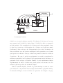
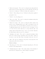
Au cours de la thèse, un titrateur automatique, complétement commandé
par ordinateur, a été assemblé dans l’atelier d’électronique du département. Les
programmes pour effectuer les titarages potentiométriques à forces ioniques constantes, ont été mis en œuvre. Le titrateur est composé de quatre burettes de
haute précision, d’une cellulle permettant une grande augmentation du volume
de la solution, d’un voltmètre de haute impédance, d’un couple d’électrodes pour
la mesure du pH (électrode de verre et une électrode de référence Ag/AgCl) et
d’un système de dégazage par l’azote. Un convertisseur analogique-digital a été
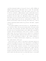
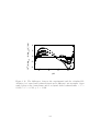
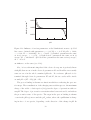
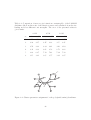
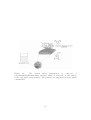
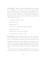
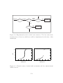
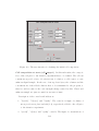
incorporé avec le voltmètre. Le nouveau titrateur ”Jonction” est représenté sur
la figure à la page suivante et décrit dans l’annexe de la thèse.
Dans le premier chapitre sont présentées la méthodologie expérimentale, ainsi
que l’analyse des données pour une évaluation de la charge présente sur une
molécule subissant l’échange de protons avec l’eau. Pour obtenir les données de
l’acidité en fonction du pH, un titrage est effectuée, durant lequel les volumes
des solutions ajoutées (HCl, KOH, KCl) et le pH, sont mesurés. L’expérience est
i
5
N2
voltmeter
A/D converter
3
2
HCl KOH KCl H2O
1
RS232
4
water
298 K
6
RS232
Le titrateur Jonction.
réalisée avec et sans la substance analysée. L’évaluation de la charge se base sur
une soustraction de l’acidité de solution blanc, à l’acidité de solution contenant la
molécule analysée. Une normalisation de la charge par la charge maximale donne
le degré de protonation; et la dépendence de ce dernier avec le pH est nommée
l’isotherme de liaison des protons. L’interprétation des courbes de titration du
blanc est effectuée avec une fonction analytique dont les paramètres sont obtenus
par régression non-linéaire. Cette procédure nous permet de vérifier les conditions
d’expérience. En outre, la précision expérimentale est verifiée en analysant les
substances standards dont les valeurs de pK apparaissent dans la littérature, en
particulier l’acide acétique et l’éthylène diamine. De très satisfaisants résultats
expérimentaux ont mis en évidence une grande précision de mesure avec des
valeurs de pK très proches des valeurs théoriques.
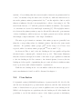
Dans le deuxième chapitre, la méthode poténtiométrique est mise en œuvre
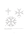
pour analyser le comportement électrostatique du dendrimère poly(amidoamine).
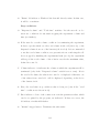
La structure chimique de cette molécule est representée sur la figure à la page
ii
suivante. Un mécanisme de protonation est proposé: il se base sur un traitement
statistique de toutes les espèces provenant de la protonation. Ceci inclut une
distinction des espèces macroscopiques et des espèces microscopiques. L’espèce
macroscopique est définie par le nombre des protons liés à la molécule, m. Ceci est
aussi appellé l’état de protonation macroscopique. Les états microscopiques sont
definis par la distribution des protons liés parmi les sites de protonation. Pour un
macro-état donné, les états microscopiques peuvent être définis en utilisant un
vecteur de dimension m, composé d’une variable binaire, si , assignée à chaque site
i. Donc, les espèces microscopiques sont definies par le vecteur si , où i = 1 à m.
L’énergie d’un état microscopique peut être modelisée en utilisant l’expansion:
1 βF ({si })
=−
pK̂i si +
ij si sj + ...
ln 10
2! i,j
i
où la sommation est effectuée sur tous les sites i, les pK̂i dénotent des constantes
de protonation microscopiques, ij dénotent des interactions entre les sites voisins,
et β = 1/kT . Toutes les probabilités statistiques des espèces macroscopiques,
ainsi que microscopiques, peuvent être calculées en utilisant l’équation ci-dessus.
Dans ce cas-là, les probabilités statistiques correspondent aux abondances des
espèces dans la solution. Par ailleurs, il est possible de calculer les constantes
de protonation macroscopiques et microscopiques. Pour un micro-état donné, les
constantes microscopiques sont la mesure de l’energie de liaison d’un proton à
un site particulier, les pK̂i sont des microconstantes du micro-état dans lequel
la molécule est complètement déprotonée, et avec ij , ils forment les paramètres
”cluster”.
La symétrie moléculaire des dendrimères permet l’établissement des
paramètres cluster, toujours selon le même principe, dont le nombre de ces
paramètres reste modéré. Il est possible de calculer toutes les constantes de protonation en utilisant ces paramètres; et réciproquement, il est possible d’obtenir
les paramètres cluster des isothermes de protonation, de manière similaire à la
régression non-linéaire.
iii
NH2
HN
O
N
N
H
N
N
N
H
N
H
N
H2N
NH2
NH2
O
O
O
H
H2N
H
H
NH2
N
NH2
N
N
N
N
N
N
N
H2N
N
NH2
N
NH2
H2N
dendrimère poly(propylèneimine)
NH2
N
H2N
NH2
H2N
NH2
N
N
N
H2N
NH2
N
NH2
H2N
H2N
N
NH2
N
H2N
NH2
N
N
N
N
H2N
N
N
H2N
NH2
N
NH2
N
H2N
H2N
N
N
dendrimère poly(amidoamine)
H2N
NH2
N
H2N
NH2
H2N
NH2
H2N
N
O
H
NH2
H
O
N
O
NH2
O
H
H
O
O
H2N
O
N
N
HN
H
O
O
H
N
N
H
HN
N
H2N
O
N
N
N
H
O
N
H
N
N
N
H
O
O
O
H
N
O
O
O
N
N
N
NH2
O
N
H
N
O
N
O
NH2
N
HN
H
N
N
H
N
NH
O
NH
O
O
N
O
H2N
H2N
HN
H
N
H2N
N
NH2
H2N
dendrimère (2,3)
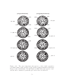
Les dendrimères étudiés de génération G2.
iv
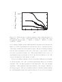
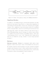
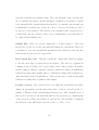
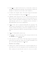
degree of protonation
1.0
m=5
0.8
m=0
m=4
0.6
0.4
0.2
0.0
2
4
6
8
10
12
pH
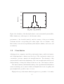
Mécanisme de protonation macroscopique de dendrimère
poly(amidoamine) G1.
Par la suite, les isothermes de protonation des six premières génerations du
dendrimère poly(amidoamine) ont été analysées par le modèle. Six paramètres
cluster sont déterminés, ceci suffisant pour une très bonne description des
courbes expérimentales. Les constantes de protonation macroscopiques sont calculées en utilisant les paramètres cluster. Puis, la connaissance des constantes
macroscopiques permet d’établir les diagrammes d’abondance des espèces macroscopiques par rapport au pH. On appelle ceci un mécanisme de protonation
macroscopique. Pour les deux premières génerations, pour lequelles le nombre
de sites reste modéré, il est même possible d’obtenir ces constantes directement par régression non-linéaire. Les valeurs obtenues de cette façon, sont en
très bon accord avec des valeurs calculées à partir des paramètres cluster. Un
mécanisme de protonation macroscopique pour la première génération de dendrimère poly(amidoamine), est présenté sur la figure ci-dessus.
Les mécanismes de protonation microscopique tiennent compte des probabilités de présence de toutes les micro-espèces, en fonction du pH. Aussi pour
v
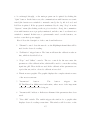
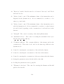
degree of protonation
1.0
0.8
PPI
2/3
0.6
1/2
0.4
(2,3)
PAMAM
0.2
0.0
2
4
6
8
10
12
pH
Isothermes de protonation de la quatrième génération des dendrimères poly(amidoamine), poly(propylèneimine) et (2,3).
les mécanismes macroscopiques, il est possible d’établir les mécanismes microscopiques en partant des paramètres cluster, cela en utilisant un traitement statistique, où l’équation 1 donne les probabilités de présence des micro-espèces.
Dans le troixième chapitre, les mécanismes de protonation sont comparés pour
trois types de dendrimères polyamine, à savoir les dendrimères poly(amidoamine),
poly(propyleneimine), et un dendrimère qui ressemble à ce dernier, mais avec une
unité centrale plus longue. Au moment de la rédaction de la présente thèse, ce
dernier dendrimère, n’est pas présent dans la litterature scientifique, car pas
encore synthétisé. Nous le nommons alors ici, dendrimère (2,3). Les isothermes de protonation pour la quatrième génération des tous les dendrimères, sont
répreésentées sur la figure ci-dessus. Les mécanismes de protonation de trois types
de dendrimères se présentent différement. Le dendrimère poly(amidoamine) est
protoné en deux étapes distinctes. Dans une première zone du pH comprise entre
10 et 7.5, les sites amines primaires sont protonés, et le reste l’est de pH 7 à
4. Dans la région de pH entre ces deux zones, apparaı̂t une micro-espèce, avec
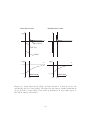
vi
poly(amidoamine)
poly(propylèneimine)
protoné
deprotoné
Micro-espèces intermédiaires présentes autour du pH=7, pour
les dendrimères poly(amidoamine) et poly(propylèneimine).
des sites amines primaires protonés, ce qui donne un plateau dans l’isotherme
de protonation au degré de protonation égal à un demi. Pour le dendrimère
poly(propylèneimine), l’isothèrme du protonation montre deux zones. Le plateu intermédiaire se situe au degré du protonation égal à deux tiers. Là, les sites
amines primaires et tous les autres sites qui se situent dans les anneaux impairs, en
comptant l’anneau avec les sites primaires comme étant le premier, sont protonés.
Le dendrimère (2,3) montre des caractéristiques dans le mécanisme de protonation, qui ont des ressemblances avec les deux dendrimères, poly(amidoamine) et
poly(propylèneimine). Pour la génération zéro, le mécanisme est proche de celui
du dendrimère poly(amidoamine), et pour les générations suivantes, il ressemble plus au mécanisme du dendrimère poly(prolpylèneimine). Les micro-espèces
intermédiaires présentes autour de pH=7, données par les mécanismes microscopiques pour les dendrimères poly(amidoamine) et poly(propylèneimine) sont
présentées sur la figure ci-dessus.
Le comportement électrostatique des surfaces colloı̈dales chargées, en absence
vii
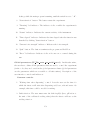
-2
surface charge (Cm )
a) pDADMAC
0.2
experiment
mixture
0.0
-0.2
b) carboxylate latex
sum a) + b)
-0.4
-0.6
4
5
6
7
pH
8
9
10
Isothermes de protonation de latex carboxil pur, de pDADMAC
pur et de latex en présence de pDADMAC adsorbé. Les courbes
représentent la somme des charges des composants purs.
et en présence d’un polyélectrolyte de charge opposée, est presenté dans les deux
derniers chapitres. Dans le chapitre 4, les isothermes de protonation des particules de latex carboxylé sont étudiée en absence et en présence du poly(chlorure de
dimethyldiallylammonium) (pDADMAC). La structure de la surface est presentée
sur la figure 4. Les isothermes du protonation pour le latex en absence du
pDADMAC, montrent le comportement typique d’une surface avec des sites acide
faible. Les isothermes de protonation du pDADMAC pur, ne montrent aucune
dépendance en charge, par rapport au pH. Par contre, les isothermes de protonation de la surface, avec le pDADMAC adsorbé, donc dans le cas d’un système
mixte, montrent une inversion de charge autour d’une certaine valeur pH. Cette
valeur peut être considérée comme le point de charge nulle (PCN), auquel de
le potentiel électrostatique de surface est égal à zéro. Les isothermes des composants purs, ainsi que de système mixte, sont présentés sur la figure à la page
suivante.
viii
Le comportement électrostatique de la surface du latex carboxylé, en présence
du pDADMAC, ressemble au comportement d’une surface d’un oxyde métallique,
par le fait de la présence du point de charge nulle.
La coı̈ncidence existe
entre celui-ci, et le point isoeléctrique trouvé par des mesures de mobilité
électrophoretique du même système. De plus, le point de charge nulle du système
mixte peut-être régi par la quantité de polyélectrolyte adsorbé. Cependant, le
point de charge nulle est présent dans les isothermes d’adsorption, mais uniquement dans les cas d’adsorptions correspondant au rapport numérique entre les
sites DADMAC et carboxylates < 1. Le comportement électrostatique de système
mixte est bien en accord avec un modèle de Stern, modifié pour la présence du
polyélectrolyte adsorbé.
Tout l’excès de charge dissout, y compris les sites DADMAC dans la solution,
peut être détecté comme un excès de charge au point de charge nulle, en observant
l’isotherme de protonation. Ceci est utile pour la détermination quantitative
d’adsorption de pDADMAC sur la surface de latex. Observée de cette manière,
l’adsorption coı̈ncide bien avec celle mesurée par l’analyse de carbone et d’azote
totaux dans la solution, comme le montre la figure à la page suivante.
Le même comportement électrostatique, précédemment observé pour le
système mixte pDADMAC-latex carboxylé, est remarquable pour le système
pDADMAC-silice. La surface de la silice exerce un comportement acide, dans
la région de pH d’étude, ce qui est montré sur la figure à la page suivante.
Cependant, quand le pDADMAC est présent à la surface, les isothermes de protonation font remarquable le point de charge nulle. Dans les expériences présentées
dans le cinquième chapitre, l’effet de la masse molaire du pDADMAC sur la
compensation de la charge de surface de la silice est étudié en comparant les
dépendances du point de charge nulle, au taux de charge du DADMAC adsorbé,
cela pour deux masses molaires, à savoir 100 et 500 kDa. La figure présentée à
la page xi ne revèle aucun effet de masse molaire.
La méthode de titrage potentiométrique s’est montrée adaptée pour effectuer
ix
-2
Adsorbed DADMAC (sites nm )
0.0
(mg m )
0.4
0.6
0.2
0.8
1.0
-2
1.0
0.8
3
diss)
0.6
2
0.4
1
(mg m-2 )
G(N
+
0.2
0
0.0
0
1
2
3
4
-2
Added DADMAC (sites nm )
Comparaison entre l’adsorption déterminée à partir des isothermes de protonation (symboles noirs), et des mesures directes
(symboles blancs).
-2
surface charge ( C m )
0.00
-0.05
-0.10
-0.15
-0.20
4
5
6
7
8
9
10
pH
Isothermes de protnation de la silice à trois forces ioniques differentes. Les courbes dénotent du modèle de Stern.
x
point of zero charge
8.5
8.0
7.5
7.0
6.5
6.0
0.2
0.4
0.6
GDADMAC (sites nm
0.8
-2
)
Point de charge nulle pour silice en présence du pDADMAC, en
fonction d’adsorption.
les études du comportement électrostatique des espèces chargées en milieux
aqueux, notamment des polyélectrolytes, des surfaces colloı̈dales, et des mélanges
des deux.
Les études des mécanismes de protonation des dendrimères polyamines ont
confirmé le modèle de protonation, suivant lequel les interactions électrostatiques
entre les sites voisins jouent un rôle très important, ainsi que les valeurs des
pK microscopiques inhérents aux sites eux-mêmes. Dans ce sens, le dendrimère
poly(amidoamine), selon lequel les sites de protonation voisins sont distants,
revèle un mécanisme de protonation determiné uniquement par les valeurs de
pK microscopiques. Au contraire, le dendrimère poly(propylèneimine), dont les
sites voisins sont plus proches, est caractérisé par un mécanisme où la protonation
des sites voisins est évitée pour raison de répulsion électrostatique.
Le comportement électrostatique d’une surface faiblement acide, s’est montré
très différent en présence, et en absence d’un polyélectrolyte de charge positive. En absence de celui-ci, le potentiel de surface est toujours négatif, et les
xi
isothermes de protonation montrent toujours une charge négative, augmentent
avec le pH. En présence du polyélectrolyte adsorbé, la charge de surface peut
être inversée par les protons liés et le potentiel de surface est égal à zéro autour
d’une valeur de pH donnée, soit au point de charge nulle. Pour cette raison, les
isothermes de liaison des protons à forces ioniques différentes, se croisent dans une
étroite région de pH. Le point de charge nulle peut être modulé par la quantité de
polyélectrolyte adsorbé. D’ailleurs, la charge mesurée au pointe de charge nulle
peut être utilisée pour déterminer le taux d’adsorption, et cela est en très bonne
adéquation avec les mesures directes. La dépendance du point de charge nulle
avec l’adsorption, pour deux masses molaires différentes, s’est montrée égale, ce
qui ne souligne aucune influence de la masse molaire du polyélectrolyte sur le
comportement électrostatique de l’interface.
xii
Introduction
Polyelectrolytes are polymers which are charged in aqueous solutions. Strong
and weak polyelectrolytes can be distinguished, one carrying strong, and the
other weak acidic or basic moieties. In water solutions, polyelectrolyte molecules
present a source of an excess charge, which stems from the conjugate pairs of
acid or base groups. The conformation of polyelectrolytes, as well as their mutual
interactions, are both closely related to the charge [1, 2]. This is important for
many of the solution properties, such as the viscosity [1, 3], aggregation stability
and aggregate structure [4], the response to the electrical and mechanical fields
[5], etc. On the other hand, the charge present on weak polyelectrolytes is tunable
by the solution conditions (pH, ionic strength), which can be used to control the
solution properties [1, 6].
The behavior of polyelectrolytes at a solid/liquid interfaces is interesting
partly due to the importance in industrial and environmental processes, and
partly due to the complexity of such systems. For example, polyelectrolytes can
be used to stabilize suspensions of particles, or induce their precipitation, which is
extensively used in industry (paper production, construction materials, food production), purification of waste waters by flocculation, etc. As well, adsorption
of polyelectrolytes at charged particles is important in production of spherical
membranes by self-assembled monolayers, which gained huge interest during the
past decade [7]. In all the above cases, a handful of colloidal properties, such
as the viscosity, colloidal stability, electrophoretic mobility, permeability of the
1
polyelectrolyte layers for small molecules etc, strongly depend upon the surface
charge. One of the goals of the present study, is to reduce the current deficit
in experimental surface charge data, and contribute to the understanding of pHdependent charging of surfaces in the presence of adsorbed polyelectrolytes.
The most straightforward method for measuring the equilibrium excess charge
in a system, which contains acid or base, is the potentiometric titration [6, 8]. The
methodology for estimating the solution excess charge from the potentiometric
titration data will be presented in the first chapter of this thesis. This will include
a thorough description of potentiometric data analysis, which will be supported
with experimental examples, the tests of precision and accuracy, and discussions
of error sources. Within the present thesis, a computer-controlled high-precision
titrator was developed. A peculiarity of this setup is the facility of performing
repeated titration experiments at constant ionic strengths, including real-time
data monitoring. A thorough technical description of this setup, directions for
programming and running, are presented in the appendix.
The focus of the second and the third chapter is on the protonation behavior
of hyperbranched polyamines in solutions. In the second chapter, the proton
binding isotherms of six different generations poly(amidoamine) dendrimers are
reported at different ionic strength. The fact that the protonation state of one site
can influence the protonation constant (pK) of another site, makes the solution
of the acid-base equilibria for polyelectrolytes more complicated than in the case
of simple or oligo-acids or bases, as was confirmed in numerous experimental
studies [1]. In the present thesis, this problem is addressed by applying a simple
site-binding model similar to the Ising model [9], which includes only several
parameters, and can be resolved by applying statistical mechanics. Within this
model, the same set of parameters can be applied for different types of molecules,
and its usefulness is demonstrated in the third chapter, where a comparison of
the detailed, microscopic charging mechanisms is presented for three types of
dendritic polyamines, namely the poly(amidoamine), poly(propyleneimine), and
2
an imaginary dendrimer, which has a structure similar to poly(propyleneimine)
dendrimer, but with a short core unit.
Fourth chapter presents a study of the charging properties of weakly acidic
carboxylate latex particles, in the presence of poly(dimethyldiallylammonium
chloride), which is a strong polycation. It is demonstrated, that the adsorbed
amount of polyelectrolyte can be inferred from the proton binding isotherms.
The applicability of the basic Stern model and a modified version of that model,
was investigated for the interpretation of the experimental data. Particularly
interesting results were obtained with the modified Stern model.
In the fifth chapter, the charging behavior of silica in the presence of adsorbed
poly(dimethyl-diallylammonium chloride) is reported. There, the focus is on
the influence of the polyelectrolyte molecular weight on the adsorption, and the
protnation behavior of silica.
3
4
Chapter 1
Potentiometric titrations at
constant ionic strengths
1.1
Introduction
In water solutions, charged species are produced through dissociation reactions.
For monoprotic acids and bases, the dissociation can be noted as:
HA H+ + A− ;
Kda =
a H+ a A−
aHA
(1.1a)
B+ + H2 O H+ + BOH ;
Kda =
aH+ aBOH
a B+
(1.1b)
where aX represents the equilibrium activity of the species X (by definition, activity of water equals unity), and Kda represents the dissociation equilibrium constant. The analytical concentrations of the species X, cX (or alternatively [X]),
are related to their activities, through the activity coefficients
γX =
aX
.
cX
(1.2)
It is also useful mentioning the mixed constants[8]:
Kd =
aH+ [A− ]
[HA]
(1.3)
5
Kd =
aH+ [BOH]
[B+ ]
(1.4)
These constants are not the true thermodynamic constants, to which they can
be related through the activity coefficients.
Equations (1.1a) and (1.1b) can be extended for polyprotic acids and bases,
which will be discussed in the chapter 3. For example, for a simple diprotic acid,
we can define the equilibirum constant for each step:
H2 A H+ + HA− ;
a
Kd,1
=
aH+ aHA−
a H2 A
(1.5a)
HA− H+ + A2− ;
a
Kd,2
=
aH+ aA2−
aHA−
(1.5b)
a
where Kd,i
denote the equilibrium constants for each step i.
The overall degree of protonation of a polyprotic acid or a base, θ, is defined
as:
1
[X]0
θ=
n
n[Xn ] − nmin
(1.6)
nmax − nmin
where n denotes the charge number of a dissociation species, nmin and nmax
are the minimum and maximum charge numbers, respectively (for acids, n is
negative, and for bases it is positive). The total concentration is given by
[X]0 =
[Xn ]
(1.7)
n
To be able to compare the concentrations of species in different solutions, the
relative concentrations, [X]/[X]0 , have to be used. The pH scale and the ionic
product of water, Kw , are defined as:
pH = − log10 aH+ , and
(1.8)
Kw = aH+ · aOH− .
(1.9)
The electroneutrality condition is one of the most important concepts for
resolving the speciation in water solutions [8]. It states that the net charge of the
6
solution as a whole equals zero:
n[Xn ] + [H+ ] − [OH− ] = 0
(1.10)
n
where [Xn ] is the analytical concentration of a species Xn . For example, if the
solution contains HCl, KOH and KCl, the electroneutrality condition reads:
[H+ ] + [K+ ] − [OH− ] − [Cl− ] = 0
(1.11)
H-Acidity and OH-Alkalinity are two quantities, which will be useful for the
calculation of the proton binding isotherms. The H-Acidity ([H-Acy]) is the
excess concentration of the protons, with respect to their concentration in a
neutral solution. For example, in a solution of acetic acid, KOH, and HCl, the
H-Acidity is:
[H-Acy] = [H+ ] − [OH− ] − [CH3 COO− ] = [Cl− ] − [K+ ]
(1.12)
Conversely, the OH-Alkalinity ([OH-Alk]), is the negative H-Acidity, for example:
[OH-Alk] = [CH3 COO− ] + [OH− ] − [H+ ] = [K+ ] − [Cl− ]
(1.13)
The activities of all the dissociation species are mutually dependent[10].
Therefore, at a fixed initial composition of the solution, the overall speciation
can be regulated by changing the activity of one single species. Since the proton
activity is easily measurable, it is convenient to express the concentrations of the
dissociation species versus pH. This also enables a comparison of the speciation
in different solutions (e.g. two different acids), with the same total concentrations
(this is the reason for which pH is called the ”master” variable[8]).
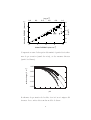
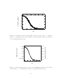
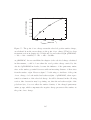
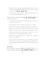
Proton binding isotherm is the dependency of the overall degree of protonation
of an acid or a base, upon pH, θ(pH) (see figure 1.1). proton binding isotherm
reflects the dissociation speciation in the solution, and is fully defined by pK̄d,i
values and the pH. For example, for acetic acid, when pH < pKd , the protonated
CH3 COOH species dominate over the deprotonated, charged CH3 COO− species.
7
degree of protonation (q)
1.0
0.8
0.6
0.4
0.2
0.0
2
4
6
8
10
pH
Figure 1.1: Example of a modeled proton binding isotherm of acetic acid at 0.1 M
ionic strength. The dashed line denotes pH=pKd =4.66[11].
When pH > pKd , the situation is reversed. In the case where the initial acid
or base concentration is proportional to some other measurable quantity, e.g.
the surface area of a particle with acidic or basic surface groups, the degree of
protonation, θ, can be replaced with the charge (in Coulombs) per surface area,
or the number (in moles) of elementary charges per surface area.
1.2
Potentiometric titration method
For the experimental determination of the proton binding isotherms, it is necessary to measure the concentrations of the charged dissociation species upon
a variation of pH in the solution. Many quantitative analytical methods can
serve for the measurement of the charged species equilibrium concentrations, for
example, spectrophotometry, NMR, conductometry, voltammetry, etc. Nevertheless, the most common way to obtain the proton binding isotherm are the
potentiometric titrations [8].
Potentiometric titration is a method, where the pH of the solution is varied by
8
controlled and measured additions of strong acid or base (e.g. HCl or KOH), and
simultaneously measured by a pH-sensitive electrode couple. The usual (minimal) experimental setup includes a burette that contains a strong acid or base
at a known concentration, a pH-measurement couple (combined glass electrode,
or separated glass and reference electrodes) with a high-impedance voltmeter,
the titration vessel and a stirrer [12]. Although the existence of the first automated titrators was reported already in the late sixties [13], the appearance of the
personal computers triggered the wide use of such systems (one example of the
first PC-controlled titrator stems from 1978 [14]). The earliest review of the automated potentiometric titration methodology, known to this author, originates
from 1968 [15].
The measured quantities are the electromotive force of the pH-sensitive electrode couple, the volumes of the strong electrolyte(s) added to the system, and the
total volume of the system (sum of the initial volume and the added volume(s) ).
From these data, the experimental titration curves (OH-Acidity versus pH) are
calculated. The term ”blank titration” will be used for a titration of a system,
which contains only strong acid and strong base counterions at concentrations
that are regulated through the additions from the burettes, protons and hydroxyle ions. For the system which, in addition to this, contains a substance for
which the proton binding isotherm should be calculated (e.g. acetic acid), the
term ”analyte titration” will be used.
In the present work, a method for automated potentiometric titrations at
constant ionic strengths was developed. The setup resembles to the Wallingford
titrator [16], and includes four burettes, each containing strong acid, strong base,
1:1 salt solution at high concentration, and water. For each titration step, the
additions of all of the burette solutions are calculated by the computer. The titrations were automatically performed at pre-defined and controlled constant ionic
strengths. In particular, this means that the pH was swept in a controlled way,
and the titration data (the glass electrode potential with respect to an Ag/AgCl
9
reference electrode, as measured by a high-impedance voltmeter, and the volumes
of the added solutions) were collected at pre-defined ionic strengths, which were
kept constant during one titration run. Successive forward and backward titration runs were performed (throughout this text, ”forward” titration means the
pH sweep from the initial to the final pre-defined pH value, and ”backward” is
the opposite direction), at different ionic strengths, which were adjusted after a
forward and backward titration cycle.
1.3
Experimental setup
In this work, with an invaluable effort of Stephane Jeannerret, a computercontrolled high-precision titration setup was built from scratch. The experience
with the Wallingford titrator [16] was very helpful to fulfill this task. The new
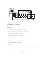
titrator is called the ”Jonction” titrator. The scheme of the Jonction titrator
setup is presented in figure 1.2. All the technical details about the ”Jonction”
titrator, and the details about the software needed to run the constant ionic
strength titrations, are presented in the appendix of this thesis.
The hardware of the Jonction titrator consists of the following (the numbers
in the list correspond to the scheme presented in fig. 1.2):
1. Four Metrohm 712 Dosimat burettes with tubings
2. pH-measurement electrode couple
3. Voltmeter (with A/D converter)
4. Titration cell
5. Pure nitrogen degassing apparatus
6. PC
10
5
N2
voltmeter
A/D converter
3
2
1
HCl KOH KCl H2O
RS232
4
water
298 K
6
RS232
Figure 1.2: Scheme of the Jonction titrator, an automated potentiometric titration setup with four burettes.
These components are connected according to the scheme depicted in figure 1.2.
The RS232 standard cables are used for the connections of the burettes and the
voltmeter to the PC.
Automatic burettes serve for high-precision dosing of all the solutions to the
titration vessel (precision of 1 µL). The additions are defined by the computer.
The bottles have to be well sealed to prevent the dissolution of CO2 .
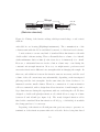
The burette tubing endings were fitted with ca. 15 cm of a narrow teflon
tubing (1/16”OD ×0.01”ID, see figure 1.3). These tubings were fitted with PEEK
fittings 1/16” ID and 1/8” ID (Alltech, cat. # 37172 and 37168, respectively),
by using the Easy Flange tool (Alltech , cat. # 35900), and joined with a PEEK
union (Alltech, cat. # 20088). Custom teflon caps with five holes were produced
in order to introduce these tubing endings into the titration cell. These caps are
produced according to the Metrohm standard for the electrode sleeves, so that
they could be placed into a standard Metrohm titration cell lid (see below).
The pH-measurement electrode couple used in this work is a separated glass,
and an Ag/AgCl reference electrode. The voltmeter and an A/D converter are
11
fittings
0.01" ID
1/16" OD
to burette
union
(Metrohm standard)
tubing ending
Figure 1.3: Fitting of the burette endings, which prevents leakage or and contact
with air.
embedded in one housing (HighImp4 instrument). The communication of the
voltmeter unit with the PC is established by means of a Labview-based software.
Jonction titrator can use any kind of standard Metrohm titration cells with
double-walls for thermostating. These cells usually have a volume of ca. 200 mL,
with a minimum solution volume (for the electrodes to be immersed) of ca. 90 mL.
However, a substantial increase in the solution volume may occur during the
constant ionic strength titrations. Moreover, one might want to perform several
successive titrations at different ionic strengths without changing the sample. In
that case, salt additions between the titration runs are necessary, and the total
volume of the cell content may vary substantially, depending on the investigated
pH range and the ionic strengths. At the same time, the electrodes have to be
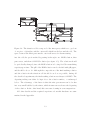
immersed even into small volumes. Therefore, construction of a custom titration
cell is recommended, with a design that allows titrations of small samples, and a
big volume increase during the experiment, without overflowing the cell. We have
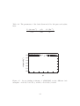
designed a double-wall plexiglas titration cell, which allows a range in volume
between 45 and 450 mL (see figure 1.4). The newly designed titration cell is
fitted with a standard Metrohm titration cell lid (e.g. 6.1414.010), from which
the clamp part has to be cut away.
Degassing of the titration cell with pure nitrogen is necessary to prevent contamination of the titration system with carbon dioxide. Before being introduced
12
Figure 1.4: The titration cell is composed of the inner part, which is scooped out
of one piece of plexiglas, and the outer wall, which is sealed around the cell,. The
space between the inner part ant the outer wall serves for thermostating.
into the cell, the gas is washed by passing it through conc. KOH solution, then
pure water, and then 0.1 M KCl solution (see figure 1.5). The solutions should
be periodically changed, since the KOH solution is loosing it’s CO2 neutralizing
capacity upon time. The pH of the KOH solution can be checked with pH-paper,
and should be above 13. Although the compositions of the final washing solution
and the solution in the titration cell should be as close as possible, during all
the described experiments, the final washing solution was always 0.1 M KCl. The
degassing tubing can either be kept above the solution surface, or submerged
below. The advantage of the latter is that the nitrogen stream can be broken
into very small bubbles by the stirrer, which in turn can accelerate the degassing
of the solution. In the other hand, this can cause foaming in some suspensions.
All other details and the acquired experience about this hardware are summarized in the Appendix.
13
N2
KOH
conc.
H 20
KCl
0.1 M
Figure 1.5: The degassing apparatus.
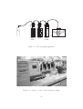
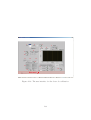
Figure 1.6: A photo of the Jonction titration setup.
14
1.4
Materials
The burette solutions are: HCl, 0.25 M, prepared form 1 M solution (Merck,
Titrisol); KOH 0.25 M, prepared from 1 M solution (J. T. Baker); KCl 3 M,
prepared from pure salt (p.a., Acros Organics), and pure decarbonated water.
The concentrations of the burette solutions can be varied according to the pH
range of interest, ionic strengths range, burette precision or some other preference.
The reported concentrations were found to be the most convenient for all the
titrations performed during this work. For all the solutions, the Millipore water
(from the Millipore A 10 deionization and purification system) was used, from
which the CO2 was removed through boiling. This procedure consists of boiling
the water for 5-10 min., and then cooling it under pure nitrogen atmosphere.
1.5
Experimental procedure
The typical experiment is performed in the following manner. First, the analyte
is added to the titration cell, which is then closed. The electrodes and all the
tubings were flushed with Millipore water, rinsed with soft paper, and mounted
to the cell. Then, the titration software is launched. The experiment is fully
controlled by the software, and from this point, the manual control over the
burettes is disabled.
First, the initial solution is automatically dosed to the titration cell, and the
pH is automatically adjusted to the pre-defined initial value. This is necessary
only in the case of analyte titrations, otherwise the initial automated dosing
will result with a solution where pH equals the initial pH. Then, a sequence of
titration steps is repeated until the final pre-defined pH value is achieved. Each
step in the titration consists of an acquirement of the reading values, namely
the electromotive force (EMF), all the added volumes, the total volume, and
additions of the burette solutions. The measurement of the pH is recorded after
15
the solution has reached thermodynamic equilibrium, which can be seen from the
drift of the electrode signal. After the final pH is achieved, the forward run is
finished, and the sense of the pH-sweep is reversed. The sequence of titration
steps is repeated in the backward-run. These two runs are repeated at all the
pre-defined ionic strengths. The experiment is terminated after all the forward
and backward titrations were effectuated at all the desired ionic strengths. The
details about all the algorithms, EMF measurement, etc. can be found in the
Appendix.
1.6
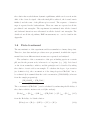
Data treatment
The automatization of the experiment enables accumulation of many data points.
Therefore, fast data analysis procedures were programmed, in which the experimental data from different titration runs were separated and analyzed.
The evaluation of the concentration of the proton-binding species at a certain
pH, used in the present work, is known for a long time (e.g. [14]). It is based
on the electroneutrality condition, and the principle can be described by taking
the solution of acetic acid as an example: To calculate the degree of protonation
(see definition 1.6), the concentration of the charged species CH3 COO− has to
be evaluated (it is assumed that the total concentration, [CH3 COOH]0 , is known
from the sample preparation):
θ=
[CH3 COOH]0 − [CH3 COO− ]
[CH3 COOH]0
(1.14)
The concentration [CH3 COO− ] can be calculated by subtracting the H-Acidty of
the solution which contains acetic acid (the analyte):
[H-Acy]HAc = [H+ ]HAc − [OH− ]HAc − [CH3 COO− ] = [Cl− ]HAc − [K+ ]HAc (1.15)
from the H-Acdity of a blank solution:
[H-Acy]blank = [H+ ]bl − [OH− ]bl = [Cl− ]bl − [K+ ]bl
16
(1.16)
-3
H-Acidity / moldm
0.01
0.00
-0.01
-0.02
2
4
6
8
10
12
pH
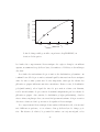
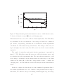
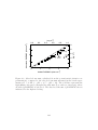
Figure 1.7: Experimental potentiometric titration curves. ◦ blank titration curve;
Acetic acid titration curve; Acetic acid charging curve.
This subtraction has to be done for all the measured pH values. The H-Acidities
are determined by the concentrations of the strong acid and base counterions
(Cl− and K+ , respectively), and thus can be calculated from the experimental
concentrations of the added strong acid and base. The charges of the ions coming from highly dissociated salts, like KCl, cancel out in the electroneutrality
expression.
The result of a typical potentiometric titration experiment, is presented in
figure 1.7. The H-Acidity versus pH curves are called the titration curves, and
are calculated from the experimental data. The curve that represents the overall
excess charge concentration in the analyte titration, with respect to the blank
solution at the same pH, is called the ”charge titration curve” or simply the
”charging curve”. It is the difference between the analyte and the blank titration
curves.
In the above figure, the data shown are from a simulated experiment, thus do
not include experimental errors. Two features of the presented data are important: First, in contrast to the proton binding isotherm (figure 1.1), the charge
17
titration curve (closed squares) is not constant at high pH: it shows a slight decrease of the [CH3 COO− ] with an increasing pH. This is due to the fact that the
concentrations depend upon the total volume, and the latter varies in the real
titration experiment (it increases with increasing pH in the presented figure).
To discard this artefact, the concentration [CH3 COO− ] can be either multiplied
by the total volume to give an amount in moles, or recalculated into the degree
of protonation through division by the total concentration [CH3 COOH]0 , which
varies with the total volume in the same way as [CH3 COO− ]. Second, the experimental points from the blank and the analyte titrations do not coincide on
the pH scale. To obtain the interpolated values, analytical function for the blank
titration curve was used, which enables computation of the OH-Alkalinities of
the blank solution at the experimental pH values from the analyte titration. The
blank titration curves were fitted to an analytical function by means of the least
squares method (a fast converging Newton method was used, acquired from the
NAG library [17]). This has enabled a comparison of the fitted parameters with
the literature values, and a cross-check of different experiments. In turn, the literature values of the blank titration curve parameters were used as a calibration
of the whole experiment. All the data analysis programming was done in the
FORTRAN language.
The volume dependency of the charging isotherms (see figure 1.7) can be
discarded by either converting the H-Acidity into the degree of protonation (1.6),
or by multiplying the H-Acidity with the total volume. In the latter case, the
amount of charge in the units of mols is obtained. As an example, figure 1.8
is showing the raw titration curves and the ”charging” curves of acetic acid.
The volume dependence is apparent from the difference between the forward
and backward titration data. Figure 1.9 is showing the two volume-independent
representations (charge in units of mols and the degree of protonation). Here,
the forward and backward titration data coincide.
The analytical expression for the electromotive force as a function of the
18
H-Acidity / mmoldm
-3
0
-5
-10
-15
-20
3
4
5
6
7
8
pH
Figure 1.8: Titration curves and charging curves of acetic acid. ◦: titration
curves; : charging curves. Open symbols: forward titration runs. Closed symbols: backward titration runs.
0.8
-1.0
0.6
-1.5
0.4
-
-[CH3COO ]· Vt/ mol
-0.5
-2.0
0.2
-3
-2.5x10
degree of protonation (q)
1.0
0.0
0.0
3
4
5
6
7
8
pH
Figure 1.9: The charging curve of acetic acid, multiplied with the total volume
of the solution. ◦: forward titration run. •: backward titration run.
19
titrant volume EMF(Va or Vb ), can be obtained from the electroneutrality condition for the blank solution (1.16). The right hand part can be expressed through
the volumes of the added strong acid and base and the total volume of the system
(Va , Vb , Vt ), and the burette concentrations of these solutions (ca , cb ):
[H-Acy]blank =
ca Va − cb Vb
10−pH 10pH−pKw
=
−
Vt
γH
γOH
(1.17)
Here, the concentrations of the H+ and OH− ions are expressed through pH, Kw ,
and the activity coefficients, according to the definition of pH (1.8) and the ionic
product of water (1.9). As an approximation we can use the common activity
coefficient (γH = γOH = γ), which accounts for the non-ideal behavior of ions
[18], and obtain:
[H-Acy]blank =
ca Va − cb Vb
1
= (10−pH − 10pH−pKw )
Vt
γ
(1.18)
The pH of the solution can be expressed through the experimentally measured
EMF, assuming the linear relationship:
EMF = E0 + ∆ · pH
(1.19)
In the above expressions, the experimentally accessible quantities are all the
volumes and the electromotive force of the electrode couple. The rest of the
quantities are parameters: ca , cb , Kw , γ , E0 , and ∆. It could be argued that the
concentrations of the burette solutions can be known from the sample preparation, but since the blank titration curve is more sensitive to these concentrations
than the accuracy of the preparation, it makes more sense fitting them.
Non-linear least squares fitting, and the cross-correlations between the blank
titration curve parameters. As mentioned in the description of the data treatment, non-linear least squares fitting of the blank titration curves is performed
in order to obtain the blank titration data at the pH values of the analyte titration curve. The advantage of this approach in front of a simple interpolation
procedure, is that in this manner, one can verify the experimental precision by
20
comparing the values of the fitted parameters with some expected, or literature
values. However, in order to obtain unambiguous values from fitting, one has to
establish the set of parameters, which can be simultaneously fitted.
In the case of the blank titration curves, the sum-of-the-squares function can
be obtained by combining equations 1.18 and 1.19:
sum =
ca Va,i − cb Vb,i
1
[
− (10(E0 −EMFi )/∆ − 10(E0 −EMFi )/∆−pKw )]2 (1.20)
Vt,i
γ
i
where i is the counter of the experimentally measured data. In the case of functions with a number of parameters that are to be fitted, the least-squares method
may not be free of ambiguities. Namely, sets of parameters may occur, which
give the same minimum in the sum-of-the-squares function (cross correlations
between parameters [19]).
Let’s now examine the sets of parameters, which can not be fitted simultaneously. For example, if we vary simultaneously the parameters γ, ca and cb (the
rest of them we keep fixed), we could find different values which give exactly
the same sum-of-the-squares (the change in the left term in equation 1.20 can
be compensated by a change in the right term, if we choose an appropriate γ).
Thus, we can not fit those parameters simultaneously. In the same manner, we
can deduce that combinations [ca , cb , pKw , E0 , ∆], and [pKw , E0 , ∆, γ] can not
be fitted. Furthermore, parameters pKw and γ could be simultaneously tuned
without affecting the sum-of-the-squares function, which means that they can
not be fitted in combination with each other.
Equation 1.20 shows that distinguishing of ca and cb is possible only if there
is a significant difference between the added amounts of strong acid and base
(Va,i and Vb,i , respectively). Otherwise, when Va,i ≈ Vb,i , the first term becomes
Va,i (ca − cb )/Vt,i . In this case, only the difference (ca − cb ) can be obtained from
fitting, and the two concentrations can not be deduced.
Having in mind the above demonstrations, the most reasonable set of fitted
parameters might be [ca or cb , γ, E0 and ∆]. The choice was to fix the acid
21
burette concentration ca , since this solution is stable regarding the dissolution
of CO2 so it’s analytical concentration is more accurate than that of the KOH.
After examining the correlations between the fitted parameters by plotting them
against each other (in this manner, the cross-correlations are ”visualized”), it was
observed that either E0 or ∆ have to be fixed (not fitted, see figures 1.16 and
1.17). The features of the blank titration curve fitting will be discussed in more
detail in section 1.8.
1.7
Results
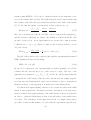
A typical result of a forward and backward blank titration at ionic strength of 0.1
M, obtained through the procedure described in section 1.6 is shown in figure 1.10.
The fitted parameters from forward titration curve are: c(KOH) = 0.2506 M,
E0 = 384.14 mV, γH = γOH = 0.82, and from the backward titration curve:
c(KOH) = 0.2505 M, E0 = 383.5 mV, γH = γOH = 0.80. Other parameters
from function 1.17 were not fitted, but fixed at the following values: c(HCl) =
0.2500 M, ∆ = −59.0 mV, Kw = 10−14 . Figure 1.11 is showing the residuals
calculated from the fitting. To discard the volume-dependency (see section 1.6),
the residuals are represented as charge in units of mols. The fitting is usually very
good, with a mean residual value (averaged over all the experimental points) of
the order of 10−6 mol see figure 1.11, which is considered as the detection limit.
Since the total volume of the system is approximately 100 mL, the detection
limit can be expressed in terms of concentration, and it equals 10−5 M. If the
solutions are prepared with care, the burettes functioning impeccably, and the
CO2 dissolution is lowered to minimum, the forward and backward curves should
coincide. Figure 1.11 nicely shows the influence of the CO2 dissolution. Here,
the fitted H-Acidities were subtracted from the experimental (as shown in the
previous figure), and multiplied with the total volume. As explained in section
1.6, the conversion of H-Acidities into amounts in moles is necessary to discard
22
-3
H-Acidity / moldm
0.001
0.000
-0.001
4
6
8
10
pH
Figure 1.10: Forward and backward blank titrations at I = 0.1 M. The markers
represent the experimental data (◦:forward,•:backward), and the lines represent
the fitted functions. The burette concentrations are: c(HCl) = 0.25 M; c(KOH) =
0.25 M; c(KCl) = 3.00 M. The aimed pH increment is 0.17 units.
the total volume dependency of the data (without this the subtracted acidities at
different pH could not be compared). The experiment was started at pH=3, and
the titration was performed up to pH=11. After the solution was exposed to a
basic pH, the CO2 started dissolving, which is apparent from an increase of the
residuals in the backward-run. The solution was again freed (to a certain extent)
of the CO2 , due to the degassing in the acidic region. This process repeats at
all the examined ionic strengths, and can be tracked in figure 1.11.
In order to test the instrument, the experimental procedures and data processing, titrations of simple acids and bases were performed. In this chapter,
the results for ethylene-diamine and acetic acid are presented. The pK-values
obtained by non-linear least squares fitting were compared with the literature
values [11]. The comparison between the fitted and the literature value serves as
an estimation of the precision of the pH-scale [14].
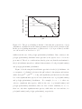
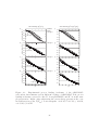
The proton binding isotherms (in terms of charge in mol units, see section
23
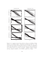
6
10 · (H-Acyexp - H-Acycalc)·Vt / mol
4
2
0
-2
-4
4
6
8
10
pH
Figure 1.11: The differences between the experimental and the calculated HAcidities for forward and backward titrations at different ionic strengths. Open
symbols denote the forward-runs, and closed symbols the backward-runs. ◦ : I =
0.1 M; : I = 0.5 M; : I = 1.0 M.
24
(H-AcyEDA-H-Acyblank)· Vt / mol
-3
4x10
3
2
1
4
6
8
10
pH
Figure 1.12: Titration curve of ethylene diamine at three different initial concentrations, at I = 0.1 M. Open symbols denote the forward, and closed
the backward titration runs. ◦ : [EDA]0 = 5.0 mM; : [EDA]0 = 2.5 mM;
: [EDA]0 = 1.0 mM.
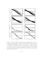
1.6) of ethylene diamine at three different initial concentrations are presented in
figure 1.12. These experiments were performed in order to verify the precision
of the charge calculated from the titration curves. The proton binding isotherms
from the same experiments, at the scale of the degree of protonation, coincide
very well, as presented in figure 1.13. This result testifies about a very good
experimental accuracy (as mentioned before, the detection limit is ca. 10−5 M),
even at concentrations of the analyte of 1 mM.
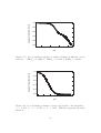
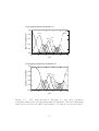
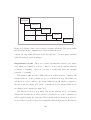
The proton binding isotherms of acetic acid at three different ionic strengths
are shown in figure 1.14. The solid lines represent the fitted proton binding
isotherms. The only fitted parameter is the mixed pKd . The ionic strength
dependence of this parameter reflects the variation of the activity coefficient of
the charged species. The proton binding isotherm of ethylene diamine exhibits
two well distinguished steps, and a plateau value at 1/2, as can be seen in figure
25
degree of protonation (q)
1.0
0.8
0.6
0.4
0.2
0.0
4
6
8
10
pH
Figure 1.13: Proton binding isotherms of ethylene diamine at different concentrations. ◦ : [EDA]0 = 1.0 mM; : [EDA]0 = 2.5 mM; : [EDA]0 = 5.0 mM.
degree of protonation (q)
1.0
0.8
0.6
0.4
0.2
0.0
3
4
5
6
7
8
pH
Figure 1.14: Proton binding isotherms of acetic acid at three ionic strengths.◦ :
I = 0.1 M; : I = 0.5 M; : I = 1.0 M. Full lines represent the fitted
functions.
26
degree of protonation (q)
1.0
0.8
0.6
0.4
0.2
0.0
4
6
8
10
12
pH
Figure 1.15: Proton binding isotherms of ethylene diamine at three ionic
strengths. ◦ : I = 0.1 M; : I = 0.5 M; : I = 1.0 M. Full lines represent the fitted functions. The fitted values of pKd are summarized in the table
1.2.
1.15. It can be noticed that the titration steps are somewhat broader than for
the acetic acid. The same treatment as for the acetic acid, can be performed
for ethylene diamine. The two pKd can be obtained by fitting, and their values
depend upon the ionic strengths. The values are summarized in table 1.1, together
with the literature values[11]. It should be noticed that the constants reported
in Martell and Smith are the concentration constants, defined as:
Kconc =
[H+ ][A− ]
[HA]
(1.21)
To compare the fitted mixed deprotonation constants (see the definitions 1.3
and 1.4) with the literature values, a correction of the mixed constants for the
activity coefficient of the proton is required. The ionic strength dependence is
more pronounced than in the case of acetic acid, which is due to the interactions
of the protonated sites, as will be discussed in chapter 2. From table 1.1, it can
be verified that the experimentally obtained deprotonation constants fit very well
with the literature values. The only exception is in the case of ethylene diamine at
27
Table 1.1: The fitted mixed deprotonation constants versus the corrected literature values.
1st step
2nd step
Substance
I /M
fit
literature [11]
fit
literature [11]
Ethylene diamine
0.1
10.02
10.02
7.21
7.02
0.5
10.14
10.15
7.44
7.43
1.0
10.21
10.29
7.54
7.56
0.1
4.70
4.66
0.5
4.62
4.62
1.0
4.64
4.67
Acetic acid
1.0 M ionic strength, where the data are less accurate due to the CO2 dissolution,
which is becoming more pronounced in the later stage of the experiment.
1.8
Discussion
The quality of the blank titration fitting is usually very good. However, this
does not necessarily mean that the obtained parameters have physical meaning.
Namely, the fitting of non-linear functions with several parameters can be ambiguous, due to the cross-correlations between the parameters [19], or the insensitivity
of the function value to a parameter in a certain range of the domain.
In order to verify the cross-correlations between the parameters E0 , ∆ and
γ which, by analytical inspection of the sum-of-the-squares function (see section
1.6), do not appear as correlated, the values obtained from fitting were plotted
against each other (figures 1.16 and 1.17). Since the absolute values of E0 and
∆ are not very significant by themselves [20], they are compared to the calibration values E0 and ∆ . In these representations, the activity coefficients γ are
28
50
E0-E0'/ mV
40
30
20
10
0
-0.2
0.0
0.2
g-g'
Figure 1.16: The cross-correlations between E0 and γ from various experiments
with two different electrode couples. Parameter E0 is presented with respect to
the value obtained from the calibration of the electrodes with standard buffers
E0 , and γ with respect to the Davies value γ . The parameters E0 and ∆ were
obtained by fitting the set [E0 , ∆, γ and cb ].
compared to the values obtained with the Davies formula (1.22). Both figures
are showing remarkable correlation between the electrode parameters and the
activity coefficient.
The parameters E0 and ∆ depend on the electrodes that are used for the
experiment. The electrode response is changing upon time, which is caused by the
changes in the electrode solutions, wearing of the glass and the ceramic diaphragm
of the reference electrode, etc. This is evident from figures 1.16 and 1.17, where
a change of the electrodes has caused a parallel shift of the data.
The fitted activity coefficients are compared with the values calculated from
the Debye-Hckel limiting law at I < 0.002 M, and Davies formula for higher ionic
strengths (see figure 1.18):
√
a· I
b
√ + ·I
γ =
2 · (1 + I) 2
(1.22)
where I is the ionic strength in M, and a and b are empirical coefficients, a = 1.022
29
D-D' / mV
0
-2
-4
-0.2
-0.1
0.0
0.1
0.2
0.3
g-g'
Figure 1.17: The cross-correlations between ∆ and γ from various experiments
with two different electrode couples. The slope ∆ is presented with respect to
the value obtained from the calibration of the electrodes with standard buffers
∆ , and γ with respect to the Davies value γ . The parameters E0 and ∆ were
obtained by fitting the set [E0 , ∆, γ and cb ].
and b is given in table 1.2. Although the fitted values are significantly scattered,
a trend is noticeable, which is similar to the prediction of the Davies equation
at low to moderate ionic strengths. At I = 1.0 M, the discrepancy is significant,
which could be due to an experimental error (these points stem from the titrations
which were performed as the last in the course of an experiment, at which stage
the system contains more dissolved CO2 ).
The parameters obtained from fitting are determinant for the experimental
pH-scale. Figure 1.19 is showing several modeled blank titration curves, with
different parameters. It can be concluded that γ influences the curve at high
and low pH. Parameter E0 shifts the titration curve parallel with the pH-scale,
while parameter ∆ causes a shift, and broadening of the titration curve. The
ionic strength influences the curve through the activity coefficients, shifting it in
high and low pH regions. The influence of pKw is growing with pH, and it is
becoming predominant over pH at pH = pKw /2. At low pH, pKw does not have
30
Table 1.2: Parameter b from the Davies formula, and the corresponding activity
coefficients.
I /M
b
log γ γ
0.1
−0.46
−0.10
0.80
0.5
−0.37
−0.12
0.76
1.0
−0.34
−0.09
0.82
1.0
0.9
g
0.8
0.7
0.6
0.5
0.0
0.2
0.4
0.6
0.8
1.0
-3
I / moldm
Figure 1.18: The activity coefficients γ obtained from the blank titration curve
fittings, versus the ionic strengths. The solid line is calculated by means of the
Davies formula.
31
-3
H-Acidity / moldm
0.001
0.000
-0.001
4
6
8
10
pH
Figure 1.19: Influence of various parameters on the blank titration curve. a) Solid
line: curve obtained with parameters ca = 0.25 M; cb = 0.25 M; pKw = 14.00;
γ = 0.90; E0 = 380.00 mV; ∆ = −59 mV. b) Dashed: parameters the same
as in a) except ; γ = 0.70. c) Dash-dotted: parameters the same as in a)
except ; E0 = 420.00 mV. d) Dotted line: parameters the same as in a) except ;
∆ = −45mV .
an influence on the curve (see 1.18).
Also, it is worth mentioning that if the electrode response is perfectly linear
with pH, then an error in the electrode parameters E0 and ∆ will not necessarily
cause an error in the whole examined pH-scale. If a reference pH-scale is determined through electrode parameters E0 and ∆ , the two scales will coincide
around pH ≈ (E0 − E0 )/(∆ − ∆ ).
The proton binding isotherms are functions which are reflecting the protonation steps. The normalization of the charging curves with respect to the maximum
charge of the acidic or basic species (1.6) gives the degree of protnation with versus pH. The degree of protonation can attain values between 0 and 1, and reflects
the protonation state of the species. The steps in the proton binding isotherms
occur in the pH regions around the pKd values, where the equilibrium is changing in favor of one species, depending on the direction of the change in pH. In
32
these regions, the solution has a higher buffering capacity [8]. The plateau values
reflect the regions in pH where one species predominates over all the others, and
the change in pH does not cause a change in speciation. Special are the proton binding isotherms of polyelectrolytes and interfaces, which are broader than
the proton binding isotherms of simple acids. These substances have a buffering
capacity in a broader pH range.
A very important feature of the proton binding isotherms are the trends with
respect to the ionic strength. These trends can be interpreted through the activity
coefficients. As a rule of a thumb, at I < 0.2 M, for acids, the pKd shift to lower
values with an increasing ionic strength. The opposite is valid for bases. The
activity coefficients actually express the deviation in the behavior of ions with
respect to the ideal solutions. This deviation is influenced by the electrostatic
potential of the counterion, which is positive in the case of a base, and thus favorable for deprotonation. The acid counterion is negative, thus electrostatically
attractive for protons, which is favorable for protonation. The electrostatic potential, experienced by the protons, depends on the ionic strength, and is higher
at lower ionic strength. At I > 0.2 M, the trend in the activity coefficients with
respect to the ionic strength is reversed, which reflects hydration layer influence
on the deviation from ideality. The hydration layer of an ion is growing with
decreasing electrostatic potential [18].
The accuracy of the experimental proton binding isotherms, and the experimental pH window, are important for assessment of the sources of errors. These
can be divided in two groups, namely error in the calculated degree of protonation, and the error of the pH scale.
The degree of protonation can be falsely calculated due to the following:
In the low and high pH regions, the H-Acidities have high values, whereas the
charge concentration, which obtained by subtracting the blank H-Acidity form
the analyte H-Acidity, can have a very a low value. In effect, one subtracts two
big numbers to obtain a small one. This is sensitive to errors because a small
33
relative error in the H-Acidities will cause a big error in the charge concentration.
This error is scaling with the initial concentration of the analyte. Thus, the initial
concentration is a determining factor for the pH window which can be experimentally studied. This error can be noticed in figure 1.13, from the broadening
of the curves at high pH (the curve at [EDA]0 = 1mM is laying slightly above
the others at high pH).
An error in the calculation of the initial concentration of the analyte can occur
due to a poor dosing control during the preparation of the analyte solution, or
e.g. due to a fact that the concentration of the stock solution is not known.
An error in the preparation of the burette solutions, causing an error in e.g.
ca , which is not fitted from the blank. An erratic preparation of the burette
solution, which concentration is fitted, will not cause any errors, since the proper
fitting will pollute the right value.
All the occurrences, which are affecting the titration curve parameters (equation 1.17 for blank titration), can be sources of errors for the pH scale, because
they have to be exactly the same for the blank and the analyte titration. These
can be changes in the electrode reading conditions between the analyte and the
blank titrations. Then, the parameters E0 and ∆ are changed, and so is the pH
scale. The error can as well arise if the experimental temperature is not the same
for the blank and the analyte titration (all the titration curve parameters are
temperature dependent to a larger or lesser extent). Furthermore, the temperature affects all the pK values, so that the proton binding isotherms at different
temperatures are not comparable. Because the literature values for pKd values
are reported at 25 ◦ C, this is the standard working temperature.
The measure for the experimental accuracy are the proton binding isotherms
of the simple acids and bases, performed at the initial concentrations of interest,
and the agreement of the fitted pKd , with the literature values. Good analyte
standards for this are the ethylene diamine and the acetic acid. Their only
disadvantage is a rather high volatility in both cases. To give an insight in the
34
0.4
frequency
0.3
0.2
0.1
0.0
-0.2
-0.1
0.0
0.1
0.2
pKd (exp) - pKd (literature)
Figure 1.20: Statistics of the fitted pK values for various standard systems (HAc,
EDA, Alanine,etc.) with respect to the literature values.
performance of the described method, and the accuracy of the proton binding
isotherms and the corresponding pKd values, figure 1.20 is a statistic of the
fitted values, from various experiments (with ethylene diamine, and acetic acid
as analytes).
1.9
Conclusion
A high-precision computer-controlled potentiometric titrator with four burettes,
and a high-impedance voltmeter was developed. The four-burette setup is very
convenient to perform constant ionic strength titrations. The advantage of this
system is that it enables the adjustments of the ionic strength in the titration cell,
without having to change the analyzed solution nor any of the burette solutions.
The data treatment, which includes fitting of the experimental blank titration
curves is advantageous, because it enables an insight in the electrode quality, and
gives insight in the possible sources of errors.
High-precision potentiometric titrations appear as a powerful tool for study35
ing the concentrations of the charged species in a solution. If all the sources of
errors are under good control, the absolute error of the determined analyte concentration is not higher than 10−6 mol. Thus, 100 mL of analyte solution with
initial concentration of 10−5 M can be easily be analyzed with only 1 % error.
The pH scale is defined by the blank titration curve parameters. The accuracy
of the pH scale, obtained in this manner, is 0.04 units.
The pH-scale, calculated from the blank titrations, can easily be verified
through titrations of substances with known dissociation constants pKd . For
this purpose, ethylene diamine and acetic acid have shown to be convenient
standards, because their proton binding isotherms exert well-defined protonation
steps. Ethylene diamine is turned out to be more convenient, since it protonates
in two well defined steps, around pH=10 and pH=7.5, so that the pH scale can
be verified in a range of several units. Furthermore, in the case of ethylene diamine, the ionic strength trends of the proton binding isotherms are sufficient to
be experimentally distinguished.
36
Chapter 2
Proton binding isotherms of
poly(amidoamine) dendrimers
2.1
Introduction
During the past two decades, dendritic polyamines have invoked great interest
of the polyelectrolyte community, due to their unique properties and potential
applications as metal complexing agents [21, 22], nanoreactors for particle synthesis [23], light harvesting devices [22], or as gene vectors [24, 25]. Their unusual
properties have been studied by numerous authors [26–39]. Their conformation
has been investigated in solution mainly by scattering [26–28] and spectroscopic
methods [29, 30], while in the adsorbed state on surfaces with AFM [31, 40]
and reflectometry [32]. Their charging behavior was studied by electrochemical
techniques [33–35], NMR [36, 37], and capillary electrophoresis[38]. The most
abundant physico-chemical studies, are those of poly(propylene imine) (PPI)
dendrimers [28, 33, 35–37], and poly(amidoamine) (PAMAM) dendrimers (see
Fig. 2.1) [26, 27, 29–31, 41]. In both cases, these dendrimers can accumulate
positive charge by protonation of the primary amines at the rim and the tertiary
amines in the interior. Their charge is thus pH dependent, whereby they are
37
positively charged at low pH and neutral at high pH.
The charging mechanisms of poly(amidoamine) and poly(propyleneimine)
dendrimers will be presented in chapter 3. In the present chapter, the aim is
to discuss experimental potentiometric titration data for poly(amidoamine) dendrimers. The interpretation of the proton binding isotherms will be presented in
terms of a site binding model, which can be used to infer both the macroscopic,
and microscopic protonation mechanisms. After introducing the model, the most
important relations for the macroscopic interpretation will be put forward. The
overall proton binding isotherms and the protonation macroconstants, calculated
by means of the site binding model, will be compared with the experimental proton binding isotherms and the macroscopic protonation constants obtained by
direct fitting of the isotherms.
2.2
Macroscopic protonation equilibria in polyelectrolyte solutions
The macroscopic protonation equilibria of polyelectrolytes is equivalent to the
protonation equilibria of polyprotic acids, where the macroscopic protonation
state, or ”macrostate”, is defined by the number of the protonated sites, m, and
the total number of protonation sites, N [6, 11]. Thus, there are N protonation
steps, and to each step, a macroscopic protonation constant is assigned:
Km =
[Hm A]
.
[H(m−1) A]aH
(2.1)
The degree of protonation, θ, can be calculated from the probabilities of the
macrostates, Pm :
N
1 θ=
mPm .
N m=1
(2.2)
38
NH2
H2N
NH2
H
N
O
NH2
N
O
HN
O
H
O
N
N
O
H
NH2
O
O
HN
H2N
NH
O
HN
O
N
N
O
O
N
N
N
H
H
NH2
NH2
H
H
NH2
O
N
N
H
N
H2N
O
N
O
H
O
H
H
O
O
O
NH2
O
H
N
N
O
H2N
H
H
N
O
N
HN
G2
O
H
N
N
H
N
H2N
HN
N
N
N
O
N
H
N
N
N
H
O
O
O
N
O
NH2
O
HN
O
O
N
N
G1
NH2
O
N
NH2
N
H2N
O
H
N
N
H
N
NH
O
HN
NH
O
O
N
O
H2N
H
N
HN
H
N
N
H2N
H2N
NH2
NH2
NH2
N
G0
O
N
N
O
N
N
N
O
H
N
H2N
H
H
O
N
H
H
N
N
O
N
NH2
H
H2N
O
O
N
N
H
O
H
N
N
H
N
H
H
NH2
NH2
Figure 2.1: Chemical structure of the zeroth, first and second generation of
poly(amidoamine) dendrimers.
39
The probability of a macrostate can be expressed through the macroscopic protonation constants:
Pm =
1+
am
H
N
m
i=1 Ki
m
m
m=1 aH
i=1
(2.3)
Ki
Equations 2.2 and 2.3 define the proton binding isotherm, θ(pH). However, the
macroscopic picture of protonation equilibria does not give information about
the distribution of bound protons among the different protonation sites. For the
convenience of the following discussions, it is also useful defining the cumulative
protonation constant for a macroscopic protonation state m:
m
K̄m =
Ki .
(2.4)
i=1
Thus, from eq. 2.3 and eq. 2.4, the macrostate probability can equivalently be
expressed as
Pm =
am
H K̄m
.
N
K̄
1 + m=1 am
m
H
(2.5)
Protonation equilibria of polyprotic acids or bases can be described with a site
binding model, which is analogous to the classical Ising model [6, 33, 36, 37, 42].
To each protonation site i, a state variable si (i = 1, 2, ..., N ) is assigned, such
that si = 1 if the site is protonated and si = 0 if the site is deprotonated. The protonation microstate is then specified by the set of state variables {s1 , s2 , ..., sN },
abbreviated as {si }. Neglecting the intermolecular interactions in a dilute solution, the free energy of a particular microstate relative to the fully deprotonated
state and for unit activity of protons can be written as an expansion
1 βF ({si })
pK̂i si +
ij si sj + ...
=−
ln 10
2!
i
i,j
(2.6)
where the sums run over all the sites, pK̂i is the microscopic protonation constant of the site i given all other sites are deprotonated, ij are pair interaction
parameters, and β = 1/kT [6, 42, 43]. The parameters ij can be related to the
40
free energy of the electrostatic repulsion between the protonated sites, Eij :
βEij
.
ln 10
ij =
(2.7)
The symmetry relation ij = ji is obeyed, and ii = 0. The multiplication of
ij with si and sj in equation 2.6 ensures that only the interactions between
the protonated sites are taken into account. It is essential to realize that within
the present model, the pair interactions act through the molecular backbone, and
their magnitude is supposed to decrease quickly with increasing distance between
the ionizable groups [44]. Thus, in the first approximation, we can consider only
the nearest-neighbor interactions, in which case the presented model is equivalent
to the Ising model [9]. Triplet, and other interactions, which in principle could
play a role, will be omitted in the present approach. The parameters pK̂i and
ij are also called the cluster parameters. The model, which is defined through
eq. 2.6 (also called the Ising Hamiltonian [42]) allows us to calculate all the
quantities related to both macroscopic, and the microscopic equilibria, from the
cluster parameters and the pH.
The total number of bound protons can be calculated for each microstate, by
m=
N
si , .
(2.8)
i=1
The probability of a particular macrostate is given by [42]:
Pm (aH ) = Ξ−1 K̄m am
H
(2.9)
where the normalization constant can be interpreted as a partition function
Ξ=
anH e−βF ({si }) .
(2.10)
{si }
and the K̄m are the cumulative protonation constants, which can be expanded
as [42]:
K̄m =
e−βF ({si }) δm, j sj .
(2.11)
{si }
41
The Kronecker symbol is denoted as δij , with δi=j = 1 and vanishes otherwise. The commonly used macroscopic step-wise dissociation constants (eq. 2.1)
can be expressed in terms of the cumulative constants as pKm = log10 Km =
log10 (K̄m /K̄m−1 ). Eq. 2.11 is also being referred to as the binding polynomial.
It becomes clear, that the site binding model can be used to express the overall
degree of protonation θ by introducing eq. 2.11 into eq. 2.5 and 2.2:
nK̄n anH
1 N
θ=
n=0
N
n
N
n=0 K̄n aH
(2.12)
Alternatively, the degree of protonation can be expressed as [42]:
θ=
aH ∂ log Ξ
N ∂aH
(2.13)
The cluster parameters can be determined by fitting the macroscopic titration
curves based on the site binding model. In contrast to the macroconstants, the
number of cluster parameters remains the same for all dendrimer generations.
For moderately sized molecules (N ≤ 30) the model was evaluated numerically
by direct enumeration of all states. For larger molecules, the model was also
solved exactly employing a transfer matrix technique. A detailed description of
this technique is given elsewhere [43].
2.3
Experimental
In this stage of the thesis, the Wallingford titrator was used to perform the
potentiometric titration experiments (for details, see appendix ). The burettes
containined 0.25 M HCl (Merck Titrisol), 0.25 M CO2 -free KOH (Baker DilutIt), 3.0 M KCl (Merck, p.a.), and pure water. All solutions were prepared with
water from a MiliQ A10 UV/UF (Milipore) system, from which the residual
CO2 was eliminated through boiling. The double-wall potentiometric plexiglass
cell was thermostatized to 25◦ C, and continuously flushed with moist CO2 -free
nitrogen. The potential between a separate glass electrode and an Ag/AgCl
42
reference electrode was measured with an high-impedance voltmeter (Microlink
PH4-S) after the drift criterion of less than 0.1 mV/min has been achieved.
A typical run started with the titration of acidified solution with KOH, and
was then back-titrated with HCl. The instrument maintains a constant ionic
strength during such a titration. The acid-base, and base-acid titrations were
repeated at ionic strengths of 0.1 M, 0.5 M, and 1.0 M. The whole sequence
of acid-base titrations at different ionic strengths was carried out automatically
within a single titration experiment.
Blank titrations were used to calibrate the glass electrode in a pH-range between 3 and 11 at ionic strengths in the range of 0.1–1.0 M. The exact base
concentration and the activity coefficients were determined by a least squares
fit. Starburst polyamidoamine (PAMAM) dendrimers (Dendritech Corporation,
Midland, USA) were titrated at total concentrations of amine groups of 10 and
20 mM. By taking the difference between the titration curves between the sample
and the blank, the charging curve of the dendrimers is obtained. The titration
curves were normalized with the known concentration of the dendrimers, and are
reported as the overall degree of protonation θ as a function of pH. The estimated
errors are ±0.04 for θ and ±0.02 for pH, respectively. The overall performance of
the system was checked with titrations of ethylenediamine and acetic acid. The
resulting ionization constants were in accord with literature values [11] within the
expected error. The dendrimer concentrations were determined from the titration
curves, and were within 2% of the values expected from the sample dosage.
2.4
Results
Potentiometric titration curves of PAMAM dendrimers at ionic strengths 0.1, 0.5
and 1.0 M in KCl for the different generations G0, G1, G2, G3, G4 and G6 are
presented in Fig. 2.2. The solid lines are model calculations to be discussed below.
The titration (or charging) curves show the characteristic dependence with the
43
Table 2.1: Cluster parameters of the site binding model of the poly(amidoamine)
dendrimers. ∆ has to be recalculated into the next-nearest neighbor parameter,
by using formula 2.14.
I (M) pK (I)
pK (III)
pK (III )
∆
0.1
9.00
6.00
6.70
0.15
2.85
0.14
0.5
9.20
6.50
7.00
0.15
2.85
0.07
1.0
9.30
6.70
7.30
0.15
2.85
0.06
ionic strength for a polybase, which is becoming more acidic with decreasing
ionic strength [6, 33]. It was further verified that the titration curves were fully
reversible and independent of the dendrimer concentration within experimental
error, indicating that dendrimer-dendrimer interactions are negligible.
The titration curves undergo a characteristic transition with increasing generation number. This transition is more clearly illustrated in Fig. 2.3, where
the titration curves for the different generations at fixed ionic strength of 0.5 M
are plotted. The smallest dendrimer G0 has 6 ionizable sites (4 primary and 2
tertiary amine groups, see Fig. 2.3 and Tab. 2.4) and shows three protonation
steps and two intermediate plateaus at θ = 4/6 and 5/6. On the other hand, the
largest dendrimer G6 with 510 ionizable sites shows two protonation steps, and an
intermediate plateau at θ = 1/2. The differences between titration curves of the
smaller dendrimers are substantial, while the titration curves of the dendrimers
G4 and above are minor, and reflect the large molecule limit. This limit, where
the titration curves becomes independent of molecular weight, is characteristic
for polyelectrolytes.
44
degree of protonation
1.0
0.8
0.6
0.4
0.2
G0
G1
G2
G3
G4
G6
0.0
degree of protonation
1.0
0.8
0.6
0.4
0.2
0.0
degree of protonation
1.0
0.8
0.6
0.4
0.2
0.0
2
4
6
8
10
12
pH
2
4
6
8
10
12
pH
Figure 2.2: Potentiometric titration curves at different ionic strengths in KCl of
PAMAM dendrimers of generations G0, G1, G2, G3, G4, and G6. Solid lines are
calculations with the site binding model.
45
degree of protonation
1.0
0.8
0.6
0.4
0.2
0.0
2
4
6
8
10
12
pH
Figure 2.3: Potentiometric titration curves of PAMAM dendrimers of generations
G0, G1, G2, G3, G4, and G6 at at ionic strength 0.1 M in KCl. Solid lines are
calculations with the site binding model.
46
2.5
Modelling and Interpretation
The macroscopic equilibria of G0 and G1 poly(amidoamine) dendrimers is described in classical terms, by fitting the pK values directly from the proton binding isotherms, and by calculating them according to the site binding model by
using the relations presented in sect. 2.2. The proton binding isotherms are interpreted in terms of the site binding model, where the degree of protonation was
calculated from the site binding model.
The macroscopic ionization constants have been determined by a least-squares
fit of the experimental titration curve (cf. eq. 2.12). The resulting macroscopic
protonation constants pKn are summarized in Tabs. 2.5 and 2.5. Six macroconstants can be determined for G0, and fourteen for G1, with reasonable confidence.
A disadvantage of this classical picture is that it is becoming impractical with increasing generation number, as the number of macroconstants increases quickly.
Furthermore, as will be discussed in chapter 3, it does not lead to insight into the
microscopic protonation mechanism of the molecule. Both disadvantages can be
overcome with the site binding model discussed now.
The cluster parameters, are illustrated in Fig. 2.4. Since the ionizable amine
groups are relatively far apart, we assume pair interactions only. Nearest neighbor
interactions act along bonds, namely one containing the amide bond with an
interaction parameter , and the ethyl chain in the center of the dendrimer with
an interaction parameter . As we shall see, a nonzero next nearest neighbor
interaction parameter between the primary amine groups must be introduced,
similarly as in the description of the charging behavior of carboxylated dendrimers
[34].
The microconstant of the primary amine groups is denoted by pK̂ (I) . For
the tertiary groups, two different microconstants must be distinguished due to
different chemical environments. The microconstant of the innermost tertiary
amines is denoted by pK̂ (III ) , while for all others the same value of pK̂ (III) will
47
Table 2.2: Comparison of macroscopic ionization constants pKm of the PAMAM
dendrimer G0 from direct fit of the titration curves and calculated from the site
binding model at different ionic strengths. The error of the presented values is
≤ 0.03 units.
0.1 M
0.5 M
1.0 M
m
fit
model
fit
model
fit
model
1
9.70
9.59
9.83
9.78
9.98
9.87
2
9.26
9.17
9.47
9.36
9.55
9.45
3
8.74
8.82
8.99
9.01
9.10
9.10
4
8.31
8.39
8.61
8.59
8.73
8.68
5
6.68
6.67
7.13
7.03
7.34
7.32
6
3.15
3.21
3.65
3.57
3.91
3.87
e''
pK (III)
e
pK (I)
pK (III')
e'
Figure 2.4: Cluster parameter assignment for the poly(amidoamine) dendrimer.
48
Table 2.3: Comparison of macroscopic ionization constants pKm of the PAMAM
dendrimer G1 from direct fit of the titration curves and calculated from the site
binding model at different ionic strengths. The error of the presented values is
≤ 0.03 units.
0.1 M
0.5 M
1.0 M
m
fit
model
fit
model
fit
model
1
9.95
9.85
10.02
10.78
10.16
10.15
2
9.70
9.50
9.87
9.72
9.76
9.79
3
9.25
9.25
9.47
9.47
9.76
9.54
4
9.19
9.05
9.34
9.27
9.28
9.34
5
8.78
8.86
9.08
9.08
9.21
9.15
6
8.68
8.65
8.92
8.88
9.07
8.95
7
8.30
8.41
8.57
8.64
8.60
8.72
8
7.96
8.07
8.29
8.30
8.47
8.39
9
7.10
7.06
7.43
7.44
7.50
7.68
10
6.36
6.35
6.91
6.81
7.21
7.00
11
5.95
5.96
6.33
6.43
6.39
6.61
12
5.55
5.61
6.17
6.08
6.56
6.27
13
5.10
5.18
5.52
5.66
5.59
5.84
14
3.07
3.20
3.51
3.57
3.66
3.86
49
be used.
While these parameters cannot be uniquely determined from a single titration
curve, they can be obtained by a simultaneous fit of G0 and G1 data. The
interaction parameters are = 0.15 and = 2.85. At this point we have set
= 0. The ionization constants increase with the ionic strength and the values
are given in Tab. 1. While a slight decrease of the interaction parameters with
increasing ionic strength could be found, the data can be equally well described
by assuming these parameters to be ionic strength independent. This approach
was adopted here for simplicity.
For the dendrimers G2, G3, G4, and G6 it was observed that a good fit cannot
be obtained without introducing an interaction between the primary amines .
While the data for all dendrimer generations can be obtained with the same cluster parameters, one further observes that increases with increasing generation
number. It was found that this dependence can be modelled as
= ∆(k − 1)
(2.14)
where k is the generation number (k > 1) and ∆ is ionic strength dependent and
is given in Tab. 1. For G0 and G1 (k = 0, 1), it was found that the interaction
parameter is negligible ( = 0). From Figs. 2.2 and 2.3 it can be inferred
that this five-parameter model describes all experimental data at a given ionic
strength to good accuracy.
The interaction parameters for the amide bond, 0.15, has not been reported in the literature before, but this value is well comparable with the corresponding value of 0.18 for an alkyl chain with the corresponding number of carbon atoms, as in hexamethyleneamine [6]. The interaction parameter 2.87
is somewhat larger than the value of 2.13 reported for ethylenediamine [6]. This
increase is probably caused by the presence of the amido side chains coordinating the nitrogen atoms. Note that decreases within increasing ionic strength,
while and are virtually ionic strength independent. This difference can be
50
understood by realizing that the nearest neighbor interactions parameterized by
and act mainly along the hydrocarbon backbone, while the interactions between the primary amines parameterized by act through the solution, and is
thus more influenced by the ionic strength due to effects of screening [6, 39]. The
trend in the increase of with the generation number is similar to the sequence
of conformations observed by small angle scattering [27]. The negligible interaction between the primary amine groups for G0 and G1 reflects the open structure
of these dendrimers, while its increase for higher generations is in line with the
increasingly compact structure of the larger dendrimers.
The microscopic ionization constants of the amine groups are generally lower
than the corresponding values for aliphatic amines, but show the same trends
otherwise. For primary amine groups, pK̂ (I) in the range 9.4–9.7 have been
reported, while for tertiary amine groups pK̂ (III) lies around 7.5 [6].
As shown in Tabs. 2 and 3, the site binding model can equally well predict
the fitted macroconstants pKn obtained from eq. 2.11. This feature illustrates
that the classical description in terms of the macroscopic equilibria is inherent
to the site binding model. In contrast to the classical picture, however, the site
binding model is capable of quantifying the protonation behavior within an entire
homologous series with a limited number of parameters.
With the site binding model one can further address the microscopic protonation mechanism in detail, as will be discussed in chapter 3.
2.6
Conclusion
Poly(aminido amine) (PAMAM) dendrimers of generations G0, G1, G2, G3, G4,
and G6 were investigated by potentiometric titrations, and the data analyzed in
terms of classical macroscopic protonation equilibria and a site binding model.
While both descriptions are equivalent, the site binding model offers further the
possibility to model the titration curves of the higher generation dendrimers,
51
and to describe all dendrimers within a common set of parameters. These parameters involve the microscopic ionization constants for each group in the fully
deprotonated state, and nearest neighbor pair interaction parameters.
52
Chapter 3
Microscopic protonation
mechanisms of dendritic
polyamines
3.1
Introduction
In the microscopic picture of protonation, the species are distinguished by both
the number of bound protons m, and their distribution among the protonation
sites [6, 45]. The studies of the protonation species at the molecular level, were
first become feasible with the development of the NMR techniques [46, 47]. This
approach has substantially become important for the studies of biologically important molecules, like oligophosphates [48, 49] or aminoacids [50]. As well, the
insight into the protonation of specific proton-binding sites within a molecule, is
important in the case of metal complexation [21, 51], or incorporation of small
molecules [52].
The microscopic charging mechanism of the dendritic polyamine molecules
is not immediately obvious, and has prompted quite some discussion in the literature [29, 31, 33, 35–37, 53]. The charging behavior of poly(propyleneimine)
53
dendrimers has been studied in substantial detail by potentiometric titrations
[33] and 15 N-NMR [36], and it was shown that these dendrimers protonate in two
steps with an intermediate plateau at a degree of protonation of 2/3. Briefly,
during the first step occurring around pH 10, the primary amine sites, and the
sites in each second shell counting from the rim, protonate. In the second step
around pH ≈ 5, the rest of the sites protonate. However, it was as well suggested
that in the poly(propyleneimine) dendrimers the primary and tertiary amines
protonate almost independently, leading to two distinct protonation steps [35].
Since in a larger dendrimer the number of primary and tertiary amine groups is
almost the same, this model would incorrectly predict an intermediate plateau
at 1/2, and not at 2/3 as observed experimentally.
The charging mechanism of poly(amidoamine) dendrimers was suggested
to involve two independent protonation steps of the primary and tertiary
amine groups [53], while others have surmised that poly(propyleneimine) and
poly(amidoamine) dendrimers should protonate similarly [31]. In this chapter,
it will be demonstrated that the protonation mechanism of poly(amidoamine)
dendrimers is very different from the poly(propyleneimine) dendrimers, and for
higher generations indeed involves the almost independent protonation of primary
and tertiary groups, which is consistent with the observed intermediate plateau
at 1/2. However, this picture is only partially correct for lower generations, since
the two innermost tertiary groups interact strongly, and protonate in two distinct
steps. Furthermore, it will be demonstrated that the protonation mechanisms of
poly(propyleneimine) and poly(amidoamine) dendrimers can be combined in the
case of a dendrimer, with a structure similar to poly(propyleneimine) dendrimer,
but with a short core carbon chain, which will be referred to as (2,3) dendrimer.
The microscopic protonation mechanisms, presented hereby, have been obtained by applying the same microscopic site binding model which was introduced in chapter 2. The cluster expansion of the free energy of protonation
[6, 33, 36, 37, 42] is used in the same manner as presented there, with a set of
54
10
11
9
4
5
12
1
8
3
2
6
7
13
protonated
deprotonated
i = 14
{si}={1,0,1,0,0,0,0,1,0,1,1,0,1,1}
Figure 3.1: One of the possible protonation microstates, for the macrostate defined with N = 14, and m = 6. The state vector si defines the microstate.
statistical-mechanical experssions, which enable the assesment of the microscopic
protonation constants, microstate probabilities, and other microscopic properties.
Again, the basis for these calculations are the cluster parameters, which in the
case of poly(amidoamine) dendrimers, are the same as presented in chapter 2.
3.2
Microscopic protonation equilibria
To define all the possible distributions of the bound protons among the protonation sites, the sites are enumerated with i, and a two-valued ”state” variable,
si = 0 or 1 (0 for deprotonated, 1 for protonated) is assigned to each site. The
microscopic protonation state (alternatively, microstate or microspecies) is defined by a state vector {si }, as demonstrated for the first generation dendrimer
molecule in figure 3.1. The microscopic protonation constant, K̂j ({si }) is attributed to an unprotonated site j when the molecule attains a microstate {si }.
The site binding model is defined in the previous chapter, through equation
2.6. However, the probability of a given microstate depends on the proton activ55
ity, aH [6, 43]:
−βF ({si })
p({si }) = Ξ−1 am
He
(3.1)
The normalization constant Ξ can be interpreted as the partition function of the
polyelectrolyte, with respect to different states of protonation:
Ξ=
−βF ({si })
am
.
He
(3.2)
{si }
As mentioned earlier, the fully unprotonated molecule is taken as the reference
state. The number of microstates for a macrostate m grows with the number of
sites, as N
[6]. The probability of a microstate, can be expressed as a product:
m
p({si }) = π({si })Pm (aH )
(3.3)
where π({si }) denotes the conditional probability of the microstate {si } within
the macrostate m. This probability is given by
−1 −βF ({si })
π({si }) = K̄m
e
(3.4)
It should be noted that the probability π({si }) does not depend on pH, and can be
easily interpreted as the mole fraction of the microspecies within a macrospecies
m.
Once all cluster parameters are known, the microscopic protonation constants,
for all the unprotonated sites within all the microstates can be calculated in a
straightforward fashion. If we label the unprotonated site with j, the association
equilibrium can be written as
A{si } + H A{si }
(3.5)
where si = si for all i = j, but sj = 0 and sj = 1. Using expansion for the
free energy (eq. 2.6), the microscopic pK value for the reaction given by eq. 3.5
follows as [42]
pK̂A{si } = pK̂i −
ij sj − ...
(3.6)
j
56
This relation defines the change in the microscopic protonation constant of a
group, in the presence of another protonated group, and reflects the group additivity concept for the estimation of protonation constants [54]. In the present
approach, the microconstants from eq. 3.6 represent secondary parameters, which
can be easily evaluated once the primary cluster parameters are known.
3.3
Protonation behavior of hyperbranched
polyamines
The concepts presented in the introduction to this chapter will be demonstrated
on several examples of branched polyamines.
These will include the zeroth
and the first generation of the poly(amidoamine) and poly(propyleneimine) dendrimers, and a dendrimer, with a structure similar to the poly(propyleneimine)
dendrimer, but with a shorter core unit. To the best knowledge of the author of
this text, the latter molecule was not yet synthesized, but could exert some interesting protonation properties to be discussed. It will be referred to as (2,3) dendrimer. The structures of poly(propyleneimine) and (2,3) dendrimers are shown
in figure 3.2, and of poly(amidoamine) dendrimer in figure 2.1. The microscopic
mechanisms estimated for the lowest two generations, will be applied to predict
the microscopic picture of protonation for the higher generations. The number
of sites for different generations can be calculated according to the formula
N = 2G+3 − 2
(3.7)
where G denotes the generation number, which is zero for the smallest molecule.
The assessment of the microscopic protonation mechanism refers to prediction of the probabilities of the microspecies with respect to pH: The macroscopic
mechanism gives the probabilities of the macrospecies. The microscopic mechanism gives the probabilities of the microspecies, and the microscopic protonation
57
constants, which can be assigned to each unprotonated site within a certain
macrostate. The probabilities of the protonation species can be interpreted in
terms of abundances in the solution. The presence of the microspecies can be
experimentally confirmed by means of spectroscopic methods, in particular NMR
[6, 36, 37], and UV-VIS and IR techniques [6]. The microstates will be presented
schematically as shown in fig. 3.1, and the macrostates will be simply denoted
with m, which is the number of bound protons to the molecule. The microscopic
mechanisms will be presented as schemes of the most prominent microspecies for
a certain macrostate, together with the according probabilities and all the microconstants. The macroscopic protonation mechanisms, will be presented in terms
of the speciation diagrams Pm (pH) (e.g. fig. 3.7), which are directly reflected in
the proton binding isotherms, as can be concluded from the eq. 2.2. In this manner, a comprehensive picture of protonation can be gained for all the molecules
studied.
The protonation mechanism can be deduced once all the cluster parameters
are assessed. The conditional probabilities of the microspecies within a certain
macrospecies can be calculated according to formula 3.4, and the microconstants
according to eq. 3.6. The difference in the microstate probabilities reflects the
difference in the free energies of microspecies, which can be calculated according
to eq. 2.6. In other words, the microstate probability is weighted by the free
energy. The proton binding isotherms can be obtained from the cluster parameters in the following manner; The energy spectrum of the molecule is calculated
according to eq. 2.6, and the cumulative macroscopic constants can then be
calculated from eq. 2.11. The degree of protonation can be obtained from the
cumulative protonation constants in a straightforward fashion, by introducng the
macrostate probabilities from eq. 2.5 into eq. 2.2.
The number of cluster parameters in the case of studied molecules is small:
a very good fitting of the proton binding isotherms of the high-generation
poly(amidoamine) dendrimers was achieved by using effectively only five differ58
H2N
NH2
NH2
H2N
N
H2N
NH2
N
H2N
NH2
N
N
N
N
NH2
NH2
NH2
NH2
H2N
H2N
N
N
H2N
NH2
N
H2N
N
N
NH2
N
N
N
NH2
N
H2N
H2N
N
N
N
N
H2N
NH2
NH2
N
H2N
G0
N
G2
NH2
N
G1
H2N
NH2
poly(propyleneimine) dendrimers
H2N
NH2
NH2
H2N
N
H2N
N
G0
H2N
NH2
N
NH2
N
N
H2N
NH2
N
NH2
H2N
NH2
N
NH2
N
N
N
N
N
NH2
H2N
N
H2N
G2
NH2
H2N
NH2
H2N
NH2
H2N
N
N
N
NH2
N
N
N
H2N
N
NH2
N
N
G1 H N
2
NH2
(2,3) dendrimers
Figure 3.2: Chemical structures of the studied molecules.
59
Table 3.1:
Cluster parameters of the site binding model for the
poly(propyleneimine) dendrimers for I = 0.1M [33].
)
pK (I)
-
9.97
0.61
1.05
-
-
9.66
9.85
0.61
1.05
1.57
8.19
7.99
9.72
9.79
0.61
1.05
1.57
3
8.19
8.02
9.71
9.70
0.61
1.05
1.57
4
8.19
7.95
9.66
9.56
0.61
1.05
1.57
generation
pK (III )
pK (III)
0
9.02
-
1
8.19
2
pK (III
ent cluster parameters (see chapter 2), and only three parameters in the case of
the zeroth generation. In the case of poly(propyleneimine) dendrimers, according
to [33], seven parameters are needed to fit the proton binding isotherms of the
second and higher generations, four for the zeroth, and six for the first generation
(see table 3.4). The procedure to obtain the cluster parameters from the experimental proton binding isotherms for poly(amidoamine) dendrimers was described
in chapter 2. For poly(propyleneimine) dendrimers, the cluster parameters were
obtained in a similar manner [33]. For (2,3) dendrimers, the cluster parameters
for the zeroth generation were taken from [44].
3.4
Poly(amidoamine) vs. poly(propyleneimine)
dendrimers
The cluster parameters, obtained by fitting the proton binding isotherms of
poly(amidoamine) dendrimers are shown in table 2.4 in chapter 2. For the
poly(propyleneimine) dendrimers, the cluster parameters were used, as reported
in [33], and the values at I = 0.1M are presented in table 3.4. For the explanation
of the seven different parameters, see figure 3.3.
60
pK(I)
pK(III'')
pK(III)
pK(III')
e
e'
Figure 3.3:
The assignment
poly(propyleneimine) dendrimers.
of
the
e''
cluster
parameters
for
the
The proton binding isotherms of poly(amidoamine) and poly(propyleneimine)
dendrimers, calculated from the cluster parameters, are presented in fig. 3.4. In
both cases, the isotherms for higher generations all follow the same curve, and a
deviation from this curve can be observed for the lowest two generations. Since
the site binding model is inherent to the type of the protonation groups and the
pair interactions, and is insensitive to the number of the protonation sites, the
appearance of the common proton binding isotherm at high generations can be
explained by the fixed respective amounts of different types of sites. For example,
for high generations of poly(amidoamine) dendrimer, there are only two types of
sites that play an important role with two distinct pK̂i values, namely the primary amine groups and the tertiary amine groups; there is only one significant
pair interaction parameter, namely . In the case of high generations, the innermost sites are greatly outnumbered by the rest, and the ratio of the primary
amine groups to the total number of sites N is approaching 1/2. Consequently,
the proton binding isotherm exerts a plateau at θ = 1/2. The proton binding
isotherms of high generations of poly(propyleneimine) dendrimers are showing a
plateau at θ = 1/3. The source of the plateau in these curves can be rationalized
61
by inspecting the most prominent microspecies, presented in fig. 3.10, as will be
discussed later.
The microscopic protonation mechanisms for the zeroth generation of
poly(amidoamine) and poly(propyleneimine) dendrimers, are shown in figures
3.5 and 3.6, respectively. In the lower part of these figures, the macroscoopic
speciation diagrams, and the overall proton binding isotherm are presented. The
proton binding isotherm shows a pronounced protonation step, at 8 < pH < 10
for poly(amidoamine), and at 9 < pH < 11 for poly(propyleneimine), where
two thirds of the sites are protonated. The microscopic mechanisms show that
the peripheral sites are protonated in the first step, due to four symmetrically
equivalent outermost groups. A common feature of the G0 mechanism for both
dendrimers is that the macrostate with four bound protons exerts three distinct
microspecies, out of which the one with the protonated primary amine groups
is largely predominant over the two with one deprotonated primary group. In
principle, another microspecies, with two unprotonated primary amine sites can
be imagined, but it turns out that the probability of that one is lower than one
per thousand. A difference in these mechanisms can be noticed regarding the
last protonation step: In the case of poly(propyleneimine) G0 dendrimer, the
inner two sites are protonated in a single step, at 5 < pH < 7. In the case of
poly(amidoamine) G0 dendrimer, the protonation of the inner two sites occurs in
two separate steps, around pH ≈ 6 and around pH ≈ 3.5. This difference can be
explained by the dependence of the pair interaction parameter on the distance
between the sites [6, 44]. For poly(propyleneimine) dendrimers, where there are
four carbon atoms in between the inner two sites, the pair interaction parameter
is lower than for the poly(amidoamine) dendrimers. These sites are separated by
only two carbon atoms.
The macrostate probability diagrams of the first generation poly(amidoamine)
and poly(propyleneimine) dendrimers are shown in fig. 3.7. The main difference is in the probabilities of the most pronounced intermediate macrostates,
62
poly(amidoamine) dendrimers
degree of protonation
1.0
0.8
G1 G2 G3
G0
0.6
G4
1/2
0.4
0.2
0.0
2
4
6
8
10
12
pH
poly(propylene) dendrimers
degree of protonation
1.0
0.8
G0
2/3
G1 G2
0.6
G3
0.4
G4
0.2
0.0
2
4
6
8
10
12
pH
Figure 3.4: Proton binding isotherms of the first five generations of the
poly(amidoamine) (top) and poly(propyleneimine) (bottom) dendrimers. The
proton binding mastercurve for poly(amidoamine) dendrimers exerts a plateau
value of θ = 1/2 at pH ≈ 7.5
63
9.00
1.2 %
8.85
8.85
3.55
1.2 %
negligible
9.00
3.55
6.40
6.70
100 %
98 %
100 %
m=5
m=4
m=0
degree of protonation
1.0
0.8
0.6
0.4
0.2
0.0
2
4
6
8
10
12
pH
Figure 3.5: Bottom: macrospeciation diagram of the zeroth generation
poly(amidoamine) dendrimer as a function of pH (broken lines), where m denotes the number of protons bound to the molecule (macrospecies). The overall
titration curve is represented with a full line. Top: the most prominent microspecies for a certain protonation step, where the micro pK values are assigned
to the unprotonated sites.
64
9.97
7.36
0.3 %
8.92
8.92
6.31
0.5 %
3.5 %
9.97
6.31
6.92
9.02
96 %
99.5 %
100 %
1.0
degree of protonation
m=4
0.8
m=5
0.6
0.4
0.2
0.0
2
4
6
8
10
12
pH
Figure 3.6: Bottom: macrospeciation diagram of the zeroth generation
poly(propyleneimine) dendrimer as a function of pH (broken lines), where m denotes the number of protons bound to the molecule (macrospecies). The overall
titration curve is represented with a full line. Top: the most prominent microspecies for a certain protonation step, where the micro pK values are assigned
to the unprotonated sites.
65
which are causing a plateau in the proton binding isotherm: In the case of
poly(amidoamine) dendrimer, it is the species with m = 8, while in the case
of poly(propyleneimine) dendrimer, it is the one with m = 10. The microscopic
mechanisms will be used to establish the most probable microstates for these
two macrostates, which play an important role for the overall proton binding
isotherms.
The
microscopic
protonation
mechanism
poly(amidoamine) dendrimer is presented in fig.
for
3.8.
the
first
generation
The most prominent
microspecies are shown with the according probabilities, and the microconstants
are presented for each unprotonated site. The increased complexity of the microscopic protonation picture for the first generation, as compared to the zeroth
generation, is not surprising, having in mind that the number of microstates
. The most prominent microspecies can
for a certain macrostate grows as N
m
be spotted by inspecting the probabilities of the microstates. In the case of
poly(amidoamine) dendrimer, these are the microspecies at m = 8, with the
protonated primary amine sites, and at m = 9, with the protonated primary,
and one of the core tertiary amine sites. These microspecies have significantly
higher probabilities than the others. For m > 9, there is one more significant
microspecies, with the protonated primary, and one of the outermost tertiary
amine sites, which is a consequence of the long chains, thus almost negligible
pair interactions, between the primary and the outermost tertiary sites.
In the case of the first generation poly(propyleneimine) dendrimer, the most
interesting microspecies is for m = 10, with protonated primary, and the innermost tertiary amine sites, as can be seen by inspecting figure 3.9. Another
difference with respect to the mechanism of the poly(amidoamine) dendrimer,
is that the difference in the probabilities of the two microspecies at m = 13, is
less pronounced, which is a consequence of a smaller difference between pK (III)
and the pK (III ) in the case of poly(propyleneimine) dendrimer. Apart from the
above differences, the microscopic mechanisms of the G1 poly(amidoamine) and
66
a) poly(amidoamine) dendrimer G1
degree of protonation
1.0
m=0
m=13
0.8
m=8
0.6
m=9
0.4
0.2
0.0
2
4
6
8
10
12
pH
b) poly(propyleneimine) dendrimer G1
degree of protonation
1.0
0.8
m=10
m=0
m=9
0.6
0.4
0.2
0.0
2
4
6
8
10
12
pH
Figure 3.7:
The macrospeciation diagrams for the first generation
poly(amidoamine) and poly(propyleneimine) dendrimers. The most important
macrospecies are denoted with m (the number of bound protons per molecule).
67
5.70
6.70
9.00
6.00
6.70
91 %
9.00
5.85
6.70
5.70
m=0
m=8
3.5 %
5.70
9.00
3.5 %
5.70
6.70
6.55
5.70
0.25 %
5.70
9.00
5.55
3.85
5.70
5.55
3.70
5.70
m=9
3.70
5.70
5.55
5.55
3.85
5.70
5.55
82 %
5.85
3.85
5.70
6.55
1.0 %
3.85
5.70
9.00
16 %
5.55
3.85
5.70
8.85
53 %
m = 10
5.55
38 %
0.25 %
5.70
6.70
6.40
8%
5.55
3.70
5.70
6.40
6.55
5.70
62 %
m = 11
4%
22 %
3.70
5.70
56 %
5.55
3.55
5.55
3.55
m = 12
3.85
5.70
6.40
40 %
5.55
5.55
11 %
2%
5.55
2%
5.55
3.55
98 %
m = 13
2%
Figure 3.8: The microscopic mechanism of the first generation poly(amidoamine)
dendrimer. The most important microspecies are presented for several distinguished macrospecies, denoted with m (see figure 3.7). A probability is assigned
to each microspecies, and the micro pK values are assigned to the unprotonated
sites.
68
poly(propyleneimine) dendrimers are similar. For example, at m = 9, there is
the same most probable microspecies, with the primary, and one innermost tertiary groups protonated. Another similarity is that at m > 9, neither of the two
mechanisms does exert clearly predominant species.
As the number of the possible microstates grows as 2N , the computation of the
detailed microscopic mechanisms, which requires calculation of the free energy for
all the microstates, is becoming increasingly consuming in terms of computation
time with an increasing generation number. In fact, for generations higher than
the second, this computation was not possible with the 1.7 GHz CPU and 512
MB RAM PC. However, the proton binding isotherm can be predicted by using
a recursive approach [43]. The sites are divided into repeating blocks, for which
the model can be solved explicitly. The protonation patterns for the blocks are
assumed to be conserved when considering the whole molecule. In spite of the
fact, that detailed mechanisms for the higher generations of dendrimers were not
calculated, the prediction of the most prominent species can be done by extending
the mechanism for the first generation. The most prominent species for the fourth
generation poly(amidoamine) and poly(propyleneimine) dendrimers are presented
in fig. 3.10.
69
8.40
6.52
8.19
9.97
9.67
8.19
8.40
7.14
69.5 %
m=0
5.47
6.53
6.52
8.19
6.52
2%
7.5 %
8.40
6.52
7.58
8.09
5.47
6.53
8.09
5.47
m=8
9.97
9.97
18.5 %
1.0 %
5.47
7.58
6.52
6.52
8.19
7.14
6.52
89 %
6.52
6.53
5.47
m=9
4%
7.04
9.97
5.47
5.47
25 %
8.40
6.53
6.52
5.47
1.5 %
m = 10
5.47
7.58
6.52
6.52
8.19
6.09
5%
71 %
2%
1%
5.47
5.47
6.53
6.52
5.47
59 %
m = 11
57 %
6.52
7.14
6.09
5.47
5.48
10 %
m = 12
37 %
5.47
5.48
6.09
1%
27 %
6.53
6.52
2%
3.5 %
5.47
5.48
67 %
m = 13
33 %
Figure 3.9:
The microscopic mechanism of the first generation
poly(propyleneimine) dendrimer.
The most important microspecies are
presented for several distinguished macrospecies, denoted with m (see figure
3.7). A probability is assigned each microspecies, and the micro pK values are
assigned to the unprotonated sites.
70
A difference in the microscopic protonation mechanisms of the higher generations of the two types of dendrimers is evident from the proton binding
isotherms for high generations. As discussed in the previous chapter, in the
case of poly(amidoamine) dendrimer, the outermost primary amine groups protonate almost randomly in the first step, at 7.5 < pH < 10. One of the innermost
sites protonates around pH ≈ 7, but for higher generations, this does not contribute significantly to the overall degree of protonation. In the second step, at
4 < pH < 7, the rest of the sites protonate almost randomly, with an exception
of one of the core sites, which protonates last, around pH ≈ 3.5. The intermediate protonation microstate with the protonated outermost primary amine
sites is prominent for the plateau value in the overall proton binding isotherm at
θ = 1/2.
In the case of the poly(propyleneimine) dendrimers, the plateau value at
θ = 1/3 is a consequence of the existence of an intermediate microspecies with
alternating protonated and deprotonated shells, which is depicted in fig. 3.10.
The primary amine groups protonate at 8.5 < pH < 11. As can be inferred from
pK (III ) and the proton binding isotherm (see fig. 3.4), the rest of the sites, leading to the shell-like intermediate structure, protonate around pH=8. This occurs
in a step which is not clearly distinguished from the protonation of the primary
amine sites. Thus, in the proton binding isotherm, this appears as a less steep
continuation of the steep part at high pH. One of the innermost tertiary amine
sites protonates next, but this contribute significantly to the overall degree of
protonation for higher generation poly(propyleneimine) dendrimers. As can be
inferred from the microconstants within the intermediate microstate, the second
step, at 3 < pH < 6, can be divided in two sub-steps, which are not distinguishable from the proton binding isotherm. In the first of these two sub-steps,
around pH ≈ 5.5, protonate the outermost tertiary amine sites, and the second
core site, while the other tertiary amine sites stay unprotonated. In the case of
the fourth generation, the latter unprotonated sites contribute only with around
71
6 % to the total number of sites. For high generations, this number is found to
converge to 8.3 %. All of these unprotonated sites protonate around pH ≈ 4.8,
which leads to the fully protonated molecule. A peculiarity of the intermediate
microspecies of the poly(propyleneimine) dendrimer, is that the protonation state
of the alternately protonated shells changes if the generation number is increased
by one.
3.5
Poly(propyleneimine)
dendrimer
with
ethylenediamine core - (2,3) dendrimer
The protonation of the poly(propyleneimine) dendrimer with ethylenediamine
core, which will be addressed to as (2,3) dendrimer, is interesting due to the
structure featured with a short ethane carbon chain in the middle of the molecule,
as shown in figure 3.2. The three carbon atom chains in the branched part are
the same as in the poly(propyleneimine) dendrimer. Therefore, this molecule
has structural features of both poly(propyleneimine) and poly(amidoamine) dendrimers. The hyperbranched part is the same as in poly(propyleneimine), and
the core as in poly(amidoamine) dendrimer. Therefore, if the site binding model,
presented for the poly(amidoamine) and poly(propyleneimine) dendrimers is correct, the microscopic protonation mechanism of the (2,3) dendrimers should exert
features of both poly(propyleneimine) and poly(amidoamine) dendrimers. For
the low (zeroth) generation, the protonation mechanism should be more similar
to the poly(amidoamine) dendrimer, and for the higher genereations, where the
branched part dominates the structure, the mechanism should be similar to the
poly(propyleneimine) dendrimer.
The cluster parameters, used to infer the protonation mechanism for the (2,3)
dendrimer from the site binding model, were used as reported in [44]. They are
listed in table 3.5 and presented in fig. 3.14 (the scheme refers to the fully
72
poly(amidoamine)
poly(propyleneimine)
9.56
6.70
9.66
10 < pH
10 < pH
6.00
9.00
7.95
6.70
5.52
8.19
6.09
7 < pH < 8
6.00
4.80
5.70
6 < pH < 8
3.55
4.80
3.5 < pH < 4.5
5.1 < pH < 5.3
pH < 3
pH < 3
Figure 3.10: The most important microspecies of the fourth generation
poly(amidoamine) (left) and the poly(propylene) (right) dendrimers, indicating
the protonation mechanism. The pH ranges in which these microspecies occur,
and the microconstants for particular protonation sites are indicated.
73
Table 3.2: Cluster parameters of the site binding model for the (2,3) dendrimer.
pK (III)
pK (I)
7.50
9.40
2.20
1.00
unprotonated molecule). It was assumed that one pK̂i value is satisfactory for all
the tertiary amine sites. As well, the pair interaction parameters were assumed
to depend purely on the spacer length between the sites. In this manner, the
parameters, which were estimated for the zeroth generation in [44], were used for
all the higher generations.
The proton binding isotherms of the first five generations of the (2,3) dendrimer are presented in fig. 3.11. Some of the features, which were established for
poly(amidoamine) and poly(propyleneimine) dendrimers, can be noticed here as
well. The proton binding isotherm of the zeroth generation is distinguished from
the other curves, which are becoming more similar to a common curve, as the
generation number is growing. The proton binding isotherm of the zeroth generation shows three distinguished titration steps, while for the higher generations,
two well distinguished steps are noticeable.
In fig. 3.12, the macroscopic speciation diagrams, and the according most
probable microspecies, are presented for the zeroth and the first generation (2,3)
dendrimer. In the case of the zeroth generation, two intermediate macrostates
are determinant for the overall proton binding isotherm, and the microscopic
protonation mechanism is very similar to that of the poly(amidoamine) dendrimer
(see fig 3.5).
The macroscopeciation diagram for the first generation (2,3) (fig. 3.12), shows
pronounced species at m = 8, m = 9 and m = 13. As a reminder, this is similar
to the macroscopic speciation of the poly(amidoamine) dendrimer. However,
the macrospecies at m = 8 is less dominant than the species at m = 9, which is
74
degree of protonation
1.0
0.8
G0
2/3
0.6
G1
G2
G3
G4
1/2
0.4
0.2
0.0
2
4
6
8
10
12
pH
Figure 3.11: The proton binding isotherms of the first five generations of (2,3)
dendrimers, calculated from the cluster parameters for the zeroth generation [44].
In the proton binding mastercurve, a plateau at θ = 2/3 is pronounced, another
one can as well be noticed at θ = 1/2.
similar as in the case of the poly(propyleneimine) dendrimer. But, contrary to the
poly(propyleneimine) dendrimer macrospeciation, the species at m = 10 is not
pronounced. The above considerations already point out, that the mechanism for
the (2,3) dendrimer may show combined characteristics of both poly(amidoamine)
and poly(propyleneimine) dendrimes.
Figure 3.13 is showing the detailed microspeciation for the (2,3) dendrimer. As
a consequence of a distinction between the pK̂i values for the primary and tertiary
amine sites (pK (I) − pK (III ) = 1.90), and significant pair interactions, the number of the significant microspecies is lower, than in the case of poly(amidoamine)
and poly(propyleneimine) dendrimers.
For example, for m = 9, there are
only two significant microspecies, while in the case of poly(amidoamine) and
poly(propyleneimine) dendrimers, there are four of them. Similarly, for m = 8,
there are only three significant microspecies, while there are four and five, for
poly(amidoamine) and poly(propyleneimine), respectively.
75
9.40
3.30
5.50
7.50
100 %
100 %
100 %
fraction macrospecies
1.0
0.8
0.6
0.4
0.2
0.0
2
4
6
8
10
12
8
10
12
pH
degree of protonation
1.0
0.8
0.6
0.4
0.2
0.0
2
4
6
pH
Figure 3.12: The macroscopic speciation diagrams, with the according most probable microspecies, for the zeroth (top) and first (bottom) generation of (2,3)
dendrimer.
76
5.50
7.50
9.40
7.50
7.50
82 %
9.40
6.50
5.30
5.50
m=8
4.50
m=0
8.40
16.5 %
6.50
5.50
7.50
1.0 %
4.50
5.30
5.50
5.50
7.50
6.50
89 %
5.50
4.30
4.50
m=9
4.50
4%
78 %
m = 10
5.30
5.50
5.50
7.50
5.50
8%
4.50
12 %
4.50
1%
4.50
4.30
5.50
8%
m = 11
26 %
4.50
5.50
5.30
4.50
3.30
4.50
3.30
8%
m = 12
2%
82 %
4.30
5.50
64 %
10 %
4.50
3.30
89 %
m = 13
11 %
Figure 3.13: The microscopic mechanism of the first generation (2,3) dendrimer. The most important microspecies are presented for several distinguished
macrospecies, denoted with m (see figure 3.7). A probability is assigned each
microspecies, and the micro pK values are assigned to the unprotonated sites.
77
The most convincing evidence that the protonation mechanism of the
(2,3) dendrimer would exert intermediate microspecies, characteristic for both
poly(amidoamine) and poly(propyleneimine) dendrimer, is demonstrated in figure
3.14. The prominent microspecies at pH ≈ 8.5 has the outermost primary amine
sites protonated, as in the case of poly(amidoamine) dendrimer. At 5 < pH < 7,
the prominent microspecies is featured with alternated protonated and deprotonated shells, as in the case of the poly(propyleneimine) dendrimer. Therefore,
the proton binding isotherm of the fourth generation of the (2,3) dendrimer (presented in fig. 3.11) is featured with a clear plateau at θ = 2/3, as in the case of
poly(propyleneimine) dendrimer. However, a less pronounced plateau at θ = 1/2
can be noticed, which is characteristic for the poly(amidoamine) dendrimers. For
the generations higher than the first, the proton binding isotherm is mostly affected by the protonation of the hyperbranched part of the molecule, which is
similar (same) as in the poly(propyleneimine) dendrimer. This is the reason why
the protonation mastercurve resembles the poly(propyleneimine) mastercurve,
with a pronounced plateau at θ = 2/3.
3.6
Conclusion
The presented site binding model is very useful for prediction of the protonation
mechanisms. Precise microscopic protonation mechanisms, which include the
probabilities of all the microstates, can be obtained for polyprotic molecules with
a very large number of sites. For this, a symmetric arrangement of the sites is
necessary, as is the case for dendrimers. However, for molecules with less than
thirty sites, the symmetric arrangement is not essential.
The microscopic protonation mechanism can be fully inferred from the cluster
parameters, which include microscopic pK values for the unprotonated molecule,
and the nearest neighbor pair interaction parameters. The pK̂i values are inherent
to a particular site, and the pair interaction parameters depend on the distance
78
7.50
5.50
9.40
7.50
11 < pH
pH = 8.5
4.50
5.50
5 < pH < 7
pH < 3
Figure 3.14: The most prominent microspecies of the (2,3) dendrimer, at pHvalues which correspond to a plateau in the overall titration curve. The microconstants of particular protonation sites are indicated.
79
between the protonated sites. Due to the symmetry of the molecule, only a limited
number of cluster parameters is necessary for an assessment of the protonation
mechanism for even very large molecules.
The poly(amidoamine) and poly(propyleneimine) dendrimers exert different
microscopic protonation mechanisms, due to a difference in the structure of the
two molecules. In the case of poly(amidoamine) dendrimers, the core carbonchain is short, while the ”arms” of the hyperbranched part are long, and vice versa
for the poly(propyleneimine) dendrimer. For poly(amidoamine) dendrimers, this
causes the mechanism to be mainly sensitive to the pK̂i parameters; the pair
interaction parameter is playing a role only for the protonation of the last core
site, at low pH. In the case of poly(propyleneimine) dendrimer, both the pK̂i ,
and the pair interaction parameters play an important role.
The
difference
in
the
microscopic
protnation
mechanisms
of
the
poly(amidoamine) and poly(propyleneimine) dendrimers affects the overall proton binding isotherm. In the case of poly(amidoamine) dendrimer, the intermediate microspecies is present at 7 < pH < 8, where the outer rim sites are
protonated, and the tertiary amine sites deprotonated. This is reflected in a
plateau in the proton binding isotherm at θ = 1/2. The protonation mechanism of the poly(propyleneimine) dendrimers is featured with an intermediate
microspecies around pH ≈ 7, where the primary amine sites, and the sites in
each second shell, counting from the outermost, are protonated. Consequently, a
plateau in the proton binding isotherm is present at θ = 2/3.
The imaginary dendrimer, which is also discussed, is built from a
short inner core unit with two carbon atoms (as in poly(amidoamine) dendrimer), and the hyperbranched part with ”arms” of three carbon atom
chains (as in poly(propyleneimine) dendrimer).
The microscopic protona-
tion mechanism shows features characteristic for both poly(amidoamine) and
poly(propyleneimine) dendrimers. At 5 < pH < 7, a microspecies with alternated protonated and deprotonated shells is present, which is the same as the one
80
observed in the poly(propyleneimine) dendrimer mechanism. A less pronounced
microspecies, present at pH ≈ 8.5, with protonated primary amine sites, is the
same as the one observed in the mechanism of the poly(amidoamine) dendrimer.
The latter microspecies is becoming more important for low generations, due to
the fact, that for higher generations, the structure of this dendrimer is dominated
by the hyperbranched part.
81
Chapter 4
Charging of carboxylated latex
particles in the presence of
pDADMAC
4.1
Introduction
Adsorption of polyelectrolytes at solid surfaces is widely used to control the colloidal stability and the hydrodynamic properties in colloidal suspensions, which
is of great interest in, for example, food and paper industry, or purification of
waste water. The colloidal stability is greatly affected by the charge carried by
particles in suspensions [55]. Furthermore, the surface charge, as well as the polyelectrolyte charge, and the concentrations of ionic species within the adsorption
layer are playing an important role for the conformation and structure of the
adsorbed or grafted polyelectrolyte layers. While the scaling theory, set forward
by de Gennes [56], led to a breakthrough in understanding the conformations of
the adsorbed polyelectrolyte layers [57, 58]. However, the ionic distributions in
the adsorbed layers still require explicit computations by means of Monte-Carlo
simulations [59].
83
An insight into the charging processes at interfaces can be gained through
the shear (or ζ-) plane potential, which can be experimentally determined from
the electrophoretic mobility or streaming potential measurements. By applying
the theory of Derjaguin, Landau, Vervey and Overbeck (DLVO) [60], an insight
about the shear plane potential may be gained from the measurements of the
aggregation rates, in the initial stages of the particle aggregation, where dimers
are formed from monomers [61]. In these studies, the aggregation rates are usually
compared with the electrophoretic mobilities, and the fast aggregation regime
typically coincides with the isoelectric point [62, 63]. As well, an evidence of
the charge distributions at solid surfaces with adsorbed polyelectrolytes can be
gained indirectly, by measuring the thickness and conformation of the adsorbed
polyelectrolyte layers [64, 65].
Potentiometric titrations provide a direct measurement of the surface charge.
In this case, the excess charge present in the solution, compensated by the protons or OH− ions, is attributed to the surface, which is acting as a conjugated
acid or base [8]. Several potentiometric titration studies of the systems consisting
of strong [66–68], and weak [69] polyelectrolytes, adsorbed on oppositely charged
surfaces, are available. In these studies, the measured amounts of adsorbed polyelectrolytes, and the net surface charge have been interpreted in terms of the
self-consistent mean field model [57]. The same approach was found appropriate
in interpretation of the layer thickness [70], the effects of the polyelectrolyte polydispersity [64], and some other effects, like the influence of the surface curvature
on the adsorption [71]. In the self-consistent mean field approach, the interactions between the ionic species, polylectrolyte segments, the solvent, and the
surface sites are treated explicitly. The relation between the surface charge and
the potential within the adsorbed layer can be solved by applying a site binding
model, which is acting as a boundary condition for solving the Poisson-Boltzmann
equation [66]. The minimum free energy, and the corresponding spatial distributions of the ions and the polyelectrolyte segments, are found by means of
84
Monte Carlo algorithms. The self-consistent mean field model invokes a number
of Flory-Huggins coefficients, which describe the interactions between different
constituents of the system (poleyelectrolyte segments, surface groups, inert electrolyte ions, solvent molecules) [72].
In this chapter, the primary aim is to present the potentiometric titration
data of the strong cationic polyelectrolyte poly(dimethyl-diallylammonium chloride) (pDADMAC), adsorbed onto carboxyl latex particles (see figure 4.1). The
fraction of the total added pDADMAC charge, which influences the surface potential (at the point of zero charge) will be evaluated from the proton binding
isotherms, and compared to the adsorbed amount of pDADMAC sites.
The experimental proton binding isotherms will be interpreted with the Stern
model [6], which is extended for a specific adsorption of oppositely charged ions
[8, 73]. The model is treating the dissociation of the surface sites through a
discrete site-binding model, similar to those which were developed for the metaloxides [74–77], with a difference that it accounts only for negative carboxylate
sites. In the case of adsorbed polyelectrolytes, the model is able to reproduce the
point of zero charge, by considering the presence of positively charged ions at the
surface, which do not undergo dissociation. The ratio of the positive polyelectrolyte sites to the negative carboxylate sites depends on the adsorbed amount.
So far, interpretation of the proton binding isotherms of the charged surfaces with
adsorbed oppositely charged polyelectrolytes has not been reported in terms of
the Stern model, which presents a mean-field approach. Our aim is to explore the
advantages and limitations of such an approach, when applied to adsorbed polyelectrolytes. The basic Stern model was first developed for the interpretation of
the ionic distributions and the corresponding electrostatic potentials near homogeneous charged surface (namely that of a mercury drop in water). Some decades
ago it became widely used for inorganic surfaces with discrete charging sites, like
metal oxides [75], and surfaces with organic acidic or basic surface moieties [74].
The applicability of the Stern model is increased through extensions, such as to
85
include the specific adsorption of ions [73, 78], or different proton binding sites
[79].
86
Figure 4.1:
The system under investigation is composed of
poly(dimethyldiallylammonium chloride) which is adsorbed on the surface
of the carboxylate latex particles. The particles are suspended in water, which
contains KCl.
87
4.2
Extension of the Basic Stern model
The pDADMAC sites can be considered to be situated in the 0-plane, or displaced
towards the solution. In the first case, the system can be described by means of
the basic Stern model. If the fixed positive charge is considered as displaced from
the surface origin, the first step towards modeling could be to place this charge at
the origin of the diffuse layer, as depicted in fig. 4.2. The latter approach will be
referred to as the modified Stern model, where the negative electrostatic potential
in the 0-plane has a higher magnitude, due to a smaller influence of the positive
pDADMAC sites. This modification is equivalent to the model which includes
the specific adsorption of the counterions, with an infinite binding constant [73]
for the cations.
The basic Stern model is a classical approach for solving the charging equilibria at homogeneous surfaces [6, 8, 74], where the interface is divided into two
compartments, namely the surface and the diffuse layer. As a consequence of the
electroneutrality condition, the charge in the diffuse layer, σd has to neutralize
the surface charge, σ0 :
σd = −σ0
(4.1)
The Gouy-Chapman equation can be invoked to calculate the potential in the
diffuse layer:
ψd = (2kT /e)arcsinh[eσd /(2kT 0 r κ)]
(4.2)
where e is the elementary charge, σd is the charge per surface area at the origin of
the diffuse layer, 0 r is the permittivity of the medium, kT the thermal energy,
and κ the inverse Debye-length:
κ=(
2e2 I 1/2
)
0 r kT
(4.3)
where, I is the ionic strength in units of number of ions per m3 . On the other
88
Modified Stern model
Basic Stern model
r(z)
z
+
z
-
G(K )+G(Cl )
G(N+ads)
G0(-COO-)
y(z)
y(z)
z
z
diffuse layer
y0
diffuse layer
yd
y0
yd
Figure 4.2: Basic Stern model (left), and the extension of that model for the
specifically adsorbed ions (right). Presented are the charge density distributions
(top), and the corresponding electrostatic potentials (bottom), with respect to
the axis normal to the surface.
89
hand, the surface charge is governed by the surface protonation equilibria:
−COOH H+ + −COO− ;
(4.4)
The corresponding deprotonation constant is
Kd =
aH+ · Γ(−COO− )
exp(qψ0 /kT ),
Γ(−COOH)
(4.5)
where ψ0 is the potential at the surface (in the plane of the surface-bound protons). Adsorbed pDADMAC sites are considered as completely dissociated, so
that pDADMAC sites are carrying a pH-independent positive charge. In the
Stern model, a potential drop between the 0-plane, and the d-plane is allowed,
such that:
CS =
σ0
ψ0 − ψd
(4.6)
where CS is the Stern layer capacitance, which can be related to the distance
between the surface and the diffuse layer plane:
d =
CS
0 r
(4.7)
The surface potential and the surface charge can be found numerically, by solving
equations 4.1-4.6
4.3
Experimental
Poly(dimethyl-diallylammonium chloride) (pDADMAC), of molecular weight
100 − 200 kDa, was purchased from Aldrich (Cat. No. 26062-79-3). The carbon and nitrogen content, and the mass percentage of the purchased solution
have been verified by the total carbon and nitrogen analysis, and were found to
agree with the formula. The solution was used without any further purification,
and was diluted to give the necessary concentration.
90
The sample of carboxyl-sulfate latex particles was kindly supplied by the
BASF company. The diameter of the particles and the polydispersity, measured
with atomic force microscopy (AFM) are 190 nm and 25.3 %, respectively. Static
and dynamic light scattering measurements of the particle diameter resulted in
a value of 250 nm. The difference between the values measured with AFM and
light scattering, is due to the fact that the diameter measured by light scattering
is intensity-weighted [80]. The surface area of the pure particles, calculated from
the AFM measurement, and taking the polydispersity into account, is 27.3 m2 g−1 .
Prior to the experiments, the particles were dialyzed against the Milli-Q water,
which was daily exchanged, until the conductivity of the outer batch water was
below ∼ 1.1 µScm−1 . For this, dialysis membranes (Spectra-pore, pore size of
500 kDa) have been used. The water, from which the CO2 was removed by boiling,
was used for the preparation of all the solutions. The burette solutions for the
potentiometric titrations, were prepared from CO2 -free KOH (Baker, Dilut-it),
HCl (Merck Titrisol) and KCl (Merck, p.a.). For the pH measurements during
the sample preparations, a combined glass electrode (purchased from Metrohm
AG) and a standard pH-meter (Metrohm 691) were used.
The potentiometric titration experiments were performed with pDADMAClatex mixtures, at five different pDADMAC loadings (see table 4.3). The final
concentration of the latex was 10 g/L in all experiments. About 20 g of a 47 g/L
latex stock solution was first mixed with pDADMAC stock solution, and the
mixture was adjusted to pH = 10. The total amount of titrated latex particles is
determinant for the accuracy of the charge determination from the potentiometric
titration (see chapter 1). The total titratable charge calculated from the latex
loading is 0.16 mmol, which means that the error of the charge determination is
lower than 2 %. The mixture was then shaken head-over-head for cca 2 minutes,
and the pH was adjusted again. Samples prepared in this way were then subjected
to potentiometric titration experiments.
Potentiometric titrations were performed with the Wallingford Titrator[16]
91
Table 4.1: Sample preparation for the titration experiments. Additions of the
pDADMAC stock solution (750 mg / L) to 20 g of 47 g/L latex suspension.
pDADMAC loading (mgm−2 )
0.15
0.40
0.65
0.85
1.00
additions pDADMAC stock solution (g)
5.0
13.9
21.5
29.0
34.4
(for a description of the automated titrators, see appendix). The experimental
set-up consists of four burettes (Metrohm Dosimat 765, cylinder volume 5 mL),
containing KOH and HCl at 0.25 M, KCl at 3 M, and water. The electromotive
force is measured with a high impedance voltmeter (Microlink PH4-S), which is
embedded in a computer interface (Microlink 3000) for the communication with
external units (burettes, stirrer). For that task, separate glass and Ag/AgCl
reference electrodes (both purchased from Metrohm AG) were used. The homemade plexiglass reaction vessel (minimum and maximum volume of the titrated
system is 45 mL, and 450 mL, respectively) was thermostatized at 25 ◦ C by an
external thermostat (Haake DC 10), and the solution was constantly degassed
with nitrogen, previously washed with concentrated KOH, water, and 0.1 M KCl
solution.
The potentiometric titration experiments are fully controlled by the computer.
First blank titrations were performed, where the electrode readings were recorded
after a drift criterion of 0.1 mV/min was satisfied, which is usually achieved in
less than 3 minutes (except in the region around pH = 7, where up to 5 minutes
were needed). Then,the samples of the composite pDADMAC-carboxylate latex
suspensions were transferred to the titration cell. The experiment begins with an
addition of HCl, KCl, and water, in order to reach the initial conditions (pH = 3,
the ionic strength of 10 mM, and total volume of 100 mL). At the beginning, the
pH is corrected in a rapid step-wise manner, through acid and base additions,
followed by the adjustment of the ionic strength to the pre-defined initial value.
92
After that, the initial conditions are achieved (pH = 3, and I = 10 mM). Then,
titration to pH = 11 is performed with a pH step of 0.4 units, which is kept
constant (see see fig. A.5 in the appendix). This is followed by a backward
titration to pH = 3 with constant dosages of 0.2 mL of HCl. In the dynamic
titration mode, the consecutive additions of acid or base are being calculated
according to the pre-defined step in pH.
The titrations of the mixture were performed in a ”rapid” manner, in order
to avoid the slow processes that were observed through long equilibration times
and high drifts (up to 1 mV/min after three minutes) of the electrode signal.
These processes could possibly be desorption, or conformational changes of the
adsorbed pDADMAC. ”Rapid” means that the maximum waiting time between
the readings was 3 minutes, in the case that the drift criterion of 0.1 mV/min
was not achieved sooner. Still, for high pDADMAC loadings and in a narrow pH
region, the drifts after 3 minutes were observed to be in the order of 5 mV/min.
The pH region of such high drifts seems to be reproducible for a certain loading.
Each addition of acid or base is followed by the ionic strength adjustment through
an addition of KCl buret solution or water. After such a forth and back titration
cycle, the ionic strength is increased. The above procedure has been repeated
until all titrations have been performed at all the pre-defined ionic strengths.
For the electrophoretic mobility measurements, the sample preparation (adsorption of pDADMAC) for the electrophoretic mobility measurements was done
in a similar way as for the potentiometric titrations.
The total amount of
pDADMAC per surface area was the same as for the titration samples, as given
in table 4.3. The final latex concentration in the samples was 5 mg / L. In order to achieve approximately the same additions of the pDADMAC and the
latex, the stock solutions were diluted to 20 mg / L and 0.32 mg / L, for latex
and pDADMAC, respectively. The final pH was varied in a range of several
pH units, such as to include an anticipated isoelectric point (assumption was
that the isoelectric point will coincide with the point of zero charge). The pH
93
was measured with a standard Metrohm 691 pH-meter, equipped with a combined pH electrode (Metrohm 6.0234.110). The values were acquired after there
was no pH-drift registered by the instrument, but for a maximum time of five
minutes. In this manner, the pH measurement conditions in the electrophoretic
mobility measurements, resemble as much as possible to these conditions in the
titrations. Electrophoretic mobilities were measured with a doppler-velocimeter
setup (Malvern Zetasizer 2000). The cell potential was set to 75 V for the measurements at I = 0.1 M , and to 100 V for the measurements at I = 0.01 M, in
order to optimize the current. The modulator frequency was set to 1 kHz. Each
data point was measured six times. For each measurement, the count rates of
the scattered photons were accumulated for 30 seconds.
The sample preparation for the batch experiments were performed in the
following manner. The latex suspension (stock solution at 0.160 mg / L) was
dialyzed against the Milli-Q water, which was daily exchanged until a constant
conductivity of cca 1 µScm−1 in the surrounding water. The pDADMAC was
used as purchased, and several stock solutions were prepared, in order to cover
a wide range of the final sample concentrations. 14.17 g of latex suspension was
mixed with a comparable volume of the pDADMAC stock solution. Then the pH
and the ionic strength were adjusted by using 0.1 M HCl and KOH solutions, and
a 1 M KCl solution. Thus, the resulting mixture has a particle concentration of
800 mg / L. After mixing, the samples were gently stirred for 24 hours. Then, the
majority of the particles was sedimented by centrifugation for 4 hours at 24000
rpm (103864 G), at 25 ◦ C (Ultra-centrifuge Beckman Coulter Avanti J30-I). The
rest of the particles were separated from the supernatant by filtration (Millex,
hydrophilic PVDF filters, pore size 0.1 µm). The supernatant was analyzed by
the total carbon and nitrogen analysis. For this, the calibration was done by
using potassuim-hydrogenphtalate and KNO3 as standards.
94
4.4
Data treatment
This section contains an important explanation of two corrections that are being performed on the raw proton binding isotherms of the composite system
pDADMAC-carboxylate latex. The first correction has to be carried out in order to subtract the charge of the free ions, added during the sample preparation.
These include K+ ions which were added to the sample as KOH in order to adjust
the pH to the adsorption value, and Cl− ions which were added with pDADMAC.
The net excess charge which stems from these strong electrolyte ions causes a shift
in the proton binding isotherms parallel with the y-axis. Therefore, the difference
between these two concentrations was subtracted from the raw proton binding
isotherms. The corrected proton binding isotherms are presented in the figure
4.3 (left).
In the second correction, the charge of the quaternary amine sites, which does
not influence the surface potential in the point of zero charge, is subtracted from
the proton binding isotherms. These sites will be referred to as not adsorbed and
+
their charge denoted [N+
diss ]. It has to be mentioned that [Ndiss ] includes the charge
of adsorbed pDADMAC sites which are displaced from the surface, wherefore
their charge is compensated by the the bulk solution ions. Their influence on
the surface potential is mitigated, and they can not be distinguished from the
dissolved sites in the proton binding isotherms. Thus, the total charge of the
added pDADMAC is split into two terms, namely adsorbed ([N+
ads ]) and dissolved
([N+
diss ]), so that the electroneutrality condition reads as:
−
−
−
+
[K+ ] + [H+ ] + [N+
ads ] + [Ndiss ] = [Cl ] + [OH ] + [∼ COO ]
(4.8)
The point of zero charge, where the surface potential equals zero, corresponds
to the common intersection point of the proton binding isotherms at different
ionic strength [78], [6]. This enables estimation of the dissolved pDADMAC
charge [N+
diss ], from the proton binding isotherms.
95
b)
surface charge (Cm - 2 )
a)
surface charge (Cm - 2 )
after subtracting ([K+]-[Cl-])
after subtracting ([N+diss]+[K+]-[Cl-])
DADMAC
loading:
0.0
0.15 mgm-2
-0.1
-0.2
f)
-0.1
G (N+diss)
-0.2
-0.3
-0.3
-0.4
-0.4
-0.5
0.40 mgm-2
0.2
g)
0.1
0.1
0.0
0.0
G
-0.1
(N+
-0.1
diss)
-0.2
-0.2
-0.3
-0.3
surface charge (Cm - 2 )
c)
0.65 mgm
-2
h) 0.3
0.3
0.2
0.2
0.1
0.1
0.0
G (N+diss)
0.0
-0.1
-0.1
-0.2
0.84 mgm-2
0.5
surface charge (Cm - 2 )
d)
0.0
i)
0.4
0.3
0.3
0.2
0.2
0.1
0.0
0.1
G (N+diss)
0.0
4
5
6
7
pH
-0.1
8
9
10
4
5
6
7
pH
8
9
10
Figure 4.3: Experimental proton binding isotherms of the pDADMACcarboxylate latex mixture at four different loadings of pDADMAC. Left: proton
binding isotherms corrected for the Cl− from pDADMAC, and K+ from the sample preparation. Right: after subtracting the excess charge present at the common intersection point, Γ(N+
diss ). Ionic strengths: ◦ 0.01 M, 0.05 M, 0.10 M,
0.50 M, ♦ 1.00 M.
96
The outcome of the second correction is shown in the figure 4.3 (right). After the correction, at the common intersection point (point of zero charge), the
surface charge equals zero. Assuming that [N+
diss ] corresponds to the charge of
dissolved pDADMAC, it makes sense subtracting this quantity from the total
added pDADMAC charge, and comparing with the adsorption isotherm, which
is shown in fig. 4.6.
Both of the above corrections were performed only in the case of the composite
pDADMAC-carboxylate latex system data. The proton binding isotherms of the
pure latex are presented as obtained by the standard data treatment, as explained
in chapter 1. In the case of pure pDADMAC titrations, the charge of the Cl−
ions, added with pDADMAC, was subtracted.
4.5
Results
The proton binding isotherms of pure carboxylate latex suspension are presented
in figure 4.4. The total amount of the titrated sites in this experiment is 0.1 mmol.
For this total amount of titratable sites, the accuracy of the calculated surface
charge equals ±2 %, within the experimental window 4 < pH < 10. Open
symbols represent experiments in which the initial pH in the titration was set
to 3.0, and the final pH to 11.0 (forward titration runs). The closed symbols
represent the opposite direction titration run. The data are showing a monotonic
dependence of the surface charge upon pH, which is typical for weakly acidic
particles [6, 61]. The maximum charge, which is achieved above pH = 10, equals
600 ± 20 mCm−2 , which corresponds to 3.74 elementary charge units per nm2 . At
low pH, typically below pH = 4, the surface charge approaches zero.
The lines in figure 4.4 represent the best fit of the basic Stern model to the
experimental data. The model parameters are presented in table 4.5. Better
fitting could not be achieved by a lower value for the Stern capacitance. The
basic Stern model in which the Stern capacitance equals infinity is equivalent to
97
-2
surface charge (Cm )
0.0
-0.1
-0.2
-0.3
-0.4
-0.5
-0.6
4
5
6
7
8
9
10
pH
Figure 4.4: The proton binding isotherm of carboxylated latex suspension at three
ionic strengths: ◦ • 0.01 M , 0.05 M , 0.10 M . The maximum surface
charge equals 600 mC m−2 . Open and closed symbols represent the forward, and
the backward titration runs, respectively. The lines represent the Basic Stern
model predictions, the parameters are presented in table 4.5.
the simple double layer model which does not include a capacitor [74, 78].
The proton binding isotherms of the pure pDADMAC solution are shown in
figure 4.5. In this case, 0.0161 g of the pure pDADMAC was titrated, which
corresponds to 0.1 mol of nitrogen (quaternary amine sites). The amount of
pDADMAC monomer units corresponds to cca 600 mC g−1 by considering every
monomer unit as one elementary charge (100 % quaternization). The curves are
showing a constant charge in the whole experimental pH range.
The results of the adsorption measurements, in the range of the loadings
which were used for the titration experiments, are presented in figure 4.6. It
can be noted that at pH = 10, all the added pDADMAC is adsorbed. The
adsorption data calculated from the proton binding isotherms are in a reasonably
good agrement with the results obtained from the batch experiemnts. Thus, it is
likely that [N+
diss ] corresponds to the pDADMAC in the solution (at least at the
point of zero charge). In the batch experiments, the adsorption of pDADMAC to
98
Table 4.2: The parameters of the basic Stern model for the pure carboxylate
latex.
Γ0 (sites nm−2 )
pKd
CS (Fm−2 )
3.74
4.20
∞
-1
charge (mCg )
0.6
0.5
0.4
0.3
0.2
0.1
0.0
4
5
6
7
8
9
10
pH
Figure 4.5: Proton binding isotherms of pDADMAC at five different ionic
strengths: ◦ 0.01 M, 0.05 M, 0.10 M, 0.0.50 M, ♦ 1.00 M.
99
the carboxylate latex particles was measured at pH = 4 and pH = 10, and at
ionic strength 0.1 M, and in the concentration range of pDADMAC as studied in
the titration experiments. The pDADMAC surface concentration of 1.0 mgm−2
corresponds to 1:1 binding of pDADMAC sites to the latex surface sites. Figure
4.6 is showing that the adsorption is higher at pH = 10 than at pH = 4.
It has to be stressed that the sample preparation for the adsorption experiments is somewhat different than for the titration experiments, which may be
a reason for the discrepancies between the measured adsorbed amounts. The
adsorbed amounts obtained from the proton binding isotherms may not be the
equilibrium amounts, since these experiments were not performed in conditions
of equilibrium adsorption. Generally, the adsorbed amounts may depend on pH
and the ionic strength, thus may vary during the titration experiments. However, from the agreement between the titration and the batch experiment data
at low loadings, it may be assumed that the adsorption of pDADMAC does not
substantially change during the titration. The fact that the charge reversal occurs in a narrow pH range, i.e. the common intersection point, points out in the
same direction. For all the model calculations which will be presented further,
the adsorbed amounts were used, as obtained from the titration experiments (the
values are listed in table 4.5). This is reasonable, because neither the charge of
the pDADMAC in the solution, nor the quaternary amine sites in the surface
vicinity that are compensated with Cl− ions, affect the protonation behavior of
latex.
The proton binding isotherms for all the studied mixtures, at several different
ionic strengths, and corrected only for the amount of chloride ions added through
pDADMAC, and potassium ions added during the sample preparation, are presented at the left side in figure 4.3. As discussed in the data treatment section,
the positive charge present at the common intersection point, [N+
diss ] could be
used to calculate the adsorbed amount of pDADMAC, by subtracting it from
the loaded pDADMAC. The proton binding isotherms to the right in figure 4.3,
100
0.0
0.2
0.8
1.0
1.0
-2
0.8
3
G(N+diss)
0.6
2
0.4
1
(mg m-2 )
Adsorbed DADMAC (sites nm )
-2
(mg m )
0.4
0.6
0.2
0
0.0
0
1
2
3
4
-2
Added DADMAC (sites nm )
Figure 4.6: Adsorbed amounts, calculated from the potentiometric titration experiments (•), compared to the adsorbed amounts measured in the batch experiments at I = 0.1M (◦ : pH = 4, : pH = 10). The solid line represents the
high-affinity adsorption (straight line with unit slope and zero intercept), where
all added pDADMAC is adsorbed. The dissolved amount of pDADMAC sites is
indicated for the highest loading.
101
which are corrected for charge [N+
diss ], will be used to test the models. In the
case of the highest loading (1.00 mg m−2 ), the common intersection point is not
clearly detectable. Therefore, [N+
diss ] could not be estimated, and calculation of
the model curves was not possible.
A comparison of the proton binding isotherms of the mixture, with the proton binding isotherms of all the components (pure latex suspension and pure
pDADMAC solution), is presented in figure 4.7. The charge of the components
(these experiments are described in figures 4.4 and 4.5), is normalized to the concentrations actually present in the mixture. The lines represent the sum of the
component charges. For this summation, the charges of pDADMAC at the pH
values of the pure latex isotherms, were computed by interpolation. A significant
disagreement between this sum, and the experimental proton binding isotherms
of the actual mixture becomes apparent.
Modeling of the proton binding isotherms of the carboxylate latex particles in
the presence of the adsorbed pDADMAC was attempted with two models, namely
the basic Stern model and the modified Stern model for the specific adsorption of
counterions. The basic Stern model, with a pKd value for the carboxylate sites
of 4.9 is not able to reproduce the curves, as can be seen in the figure 4.8 (left
column). The Stern capacitance influences the slope of the curves (the lower the
capacitance, the lower the slope), but does not affect the position of the point of
zero charge, which can in this case not be correctly reproduced in the modeled
curves.
Much better descritpion was achieved with the modified Stern model, which
was described in the introduction to this chapter. The parameters that resulted
in the best fitting are presented in the table 4.3. The fitting was also attempted
with a protonation constant value of 4.2 (as obtained from the fitting of the
proton binding isotherms of the pure latex suspension, see figure 4.4 and table
4.2), but resulted with worse fits.
The proton binding isotherms, as compared to the pH-dependencies of the
102
-2
surface charge (Cm )
a) pDADMAC
0.2
experiment
mixture
0.0
-0.2
b) carboxylate latex
sum a) + b)
-0.4
-0.6
4
5
6
7
pH
8
9
10
Figure 4.7: Proton binding isotherms of carboxylated latex suspension in the presence of pDADAMAC, at a loading of 0.65 mgm−2 , at five different ionic strengths.
Closed symbols represent the isotherms of pure components (pure pDADMAC
solution in the upper part, and the pure latex suspension in the lower part of
the graph), recalculated to the concentrations present in the mixture. The lines
represent the sum of the (interpolated) isotherms of the pure components. Open
symbols represent the experimental proton binding isotherm of the mixture. Ionic
strengths: ◦ • 0.01 M, 0.05 M, 0.10 M.
103
Basic Stern model
Modified Stern model
e)
0.0
-2
surface charge (Cm )
a)
-0.1
-0.2
-0.3
-0.4
-0.5
-2
surface charge (Cm )
b)
f)
0.1
0.0
-0.1
-0.2
-0.3
-2
surface charge (Cm )
c) 0.3
g)
0.2
0.1
0.0
-0.1
-0.2
-2
surface charge (Cm )
d)
h)
0.3
0.2
0.1
0.0
-0.1
4
5
6
7
8
9
10
pH
4
5
6
7
8
9
10
pH
Figure 4.8: A comparison between the predictions of the proton binding isotherms
(lines), for four different surface compositions (as indicated in table 4.5), of the
basic Stern model (left), and the modified Stern model (right). The parameters
used for the basic Stern model calculations are the same as for the modified Stern
model (listed in table 4.5), except for the Stern capacitances (given in Fm−2 ):
a) ∞, b) 5.00, c)1.50, d) 1.00. Ionic strengths: ◦, full line: 0.01 M; , dashed:
0.05 M; , dash-dot: 0.10 M; , dot: 0.50 M; ♦, dash-dot-dot: 1.00 M.
104
Table 4.3: The parameters used to calculate the modified Stern model predictions
of the proton binding isotherms for different pDADMAC-latex mixture compositions. The adsorbed and dissolved amounts were calculated from the charge at
point of zero charge. Stern capacitance is denoted CS .
pDADMAC
Γ(N+
ads )
Γ(N+
diss )
loading (sites nm−2 )
(sites nm−2 )
(sites nm−2 )
CS (Fm−2 )
pHpzc
0.56
0.35
0.21
6.95
4.00
1.50
1.18
0.32
3.02
5.82
2.44
1.91
0.53
2.90
6.84
3.15
2.27
0.88
2.40
7.76
1.00
-
-
-
> 9.0
electrophoretic mobilities, are presented in figure 4.9. The lines in the top figures were calculated by means of the modified Stern model, as described in the
introduction to this chapter, and using the parameters listed in table 4.3. The
coincidence between the point of zero charge, as obtained from the proton binding isotherms, and the isoelectric points, as obtained from the electrophoretic
mobility measurements, is obvious. The lines in the bottom figures represent the
predictions of the O’Brien [81] and White theory for the electrophoretic mobilities. For this, the shear-plane potential was calculated from the surface potential
(ψ0 ) by means of the Gouy-Chapman theory (the fitted shear-plane distances are
given in table 4.4). The calculation of the electrophoretic mobilities from the
shear-plane potential is described in the paper of O’Brien and White. In the
present work, the mobilities have been obtained by interpolation, from databases
which contain mobilities for various values of the shear-plane potential.
105
b)
0.0
0.1
-2
surface charge (Cm )
a)
-0.1
0.0
-0.2
-0.1
-0.3
-0.2
-0.4
-0.3
-0.5
c)
-2
surface charge (Cm )
0.3
d)
0.3
0.2
0.2
0.1
0.1
0.0
0.0
-0.1
-0.1
-0.2
electrophoretic mobility
-8 2 -1 -1
(10 m V s )
e)
f)
4
4
2
2
0
0
-2
-2
-4
-4
-6
electrophoretic mobility
-8 2 -1 -1
(10 m V s )
g)
h)
4
4
2
2
0
0
-2
-2
-4
-4
4
5
6
7
pH
8
9
10
4
5
6
7
pH
8
9
10
Figure 4.9: Proton binding isotherms (a-d) and pH-dependence of the electrophoretic mobility (e-h) of carboxylated latex suspension in the presence
of pDADAMAC. pDADMAC loadings: 0.15 mg / m2 (a,e); 0.40 mg / m2 (b,f);
0.65 mg / m2 (c,g); 0.84 mg / m2 (d,h). Ionic strengths: ◦ 0.01 M, 0.05 M,
0.10 M, 0.25 M, ♦ 1.00 M. The lines in the figures (e-d) represent the
the modified Stern model predictions (parameters listed in table 4.5). The lines
in figures (e-h) represent the O’Brien and White model prediction (shear plane
distance listed in table 4.5).
106
Table 4.4: The shear plane distances obtained by fitting the experimental electrophoretic mobilities according to the O’Brien and White theory [81].
pDADMAC loading (mgm−2 ) 0.15
shear plane distance (nm)
4.6
0.20
0.40
0.65
0.84
0.30
0.32
0.40
Discussion
The adsorption isotherms from the batch experiments (figure 4.6) at pH = 10
are showing a high-affinity equilibrium adsorption behavior of pDADMAC at the
carboxylate latex surface. Small deviations from this behavior are possibly due
to a fact that the equilibrium was not reached. High-affinity adsorption is a
regime, where the adsorption is quantitative up to a saturation limit, after which
the adsorbed amount can not be further increased, but remains constant upon
further additions. In the present case, when the adsorption is carried out at
pH = 10, the saturation limit is not reached in the range of loadings examined.
The presence of the adsorbed oppositely charged polyelectrolyte is promoting
the development of the negative charge at the latex surface, which is in turn
promoting the adsorption [69, 82, 83]. However, at pH = 4, lower adsorption
was observed, and in this case the adsorption is not of the high-affinity type.
The increased adsorption at higher pH is not surprising, having in mind that
the charge, present at the surface of the carboxylate latex particles is increasing
with an increasing pH. This points out that in the studied (low) range of loading,
adsorption of pDADMAC to the carboxylate latex surface can be regarded as an
example of the screening-reduced regime, according to de Keizer et al. [84].
The proton binding isotherms of the pure latex suspension (fig. 4.4) are showing typical protonation behavior for weakly acidic particles [6, 8]. The experimental data could be reasonably well fitted with the simple double layer model.
The value of 4.2, obtained for the microscopic pKd of a carboxylic surface site,
107
seems a bit too low (the reported values are usually around 4.9 [61], [85] and for
comparison, the pKd of acetic acid in solution is ∼ 4.6 [11]). However, this was
the highest value that could be used in order to describe the data in terms of the
double layer model, or the basic Stern layer model. A possible source for such a
low pKd value might be the specific adsorption of negative counterions (in this
case Cl− [8]). As well, a higher surface charge (∼ 600 mCm−2 ) than usual has
been observed [61, 85], which could be due to the surface roughness.
The proton binding isotherms of pDADMAC (figure 4.5) are showing a fairly
constant charge of the quaternary amine groups, upon the variation of pH. It has
to be stressed that pDADMAC does not contribute to the total net charge in the
solution, since the charge of the quaternary amine groups is fully compensated
by the charge of the counterions Cl− , and in this respect, pDADMAC acts as a
monovalent strong electrolyte. However, when adsorbed to the carboxylate latex
surface, these counterions are to a certain extent depleted from pDADMAC,
which gives rise to the positive surface charge of the adsorbed pDADMAC [67].
Although the adsorption isotherms from the batch experiments are showing a
dependence of the equilibrium adsorbed amount on the pH, a very good reversibility of the titration curves was achieved by fast titration experiments, which was
established by comparing the data from the forward and backward titration runs
at same pH and ionic strength. This, and the fact that the common intersection
points can be easily recognized in the proton binding isotherms, is leading to a
conclusion that the adsorbed amounts of pDADMAC did not change to a great
extent during the titrations.
The main feature of the proton binding isotherms of the carboxylate latex
particles in the presence of adsorbed pDADMAC, is the common intersection
point of the curves at different ionic strengths, which indicates the reversal of
the surface charge. This can be clearly explained by inspecting figure 4.7. If the
latex particles and pDADMAC would be separated in the water medium (with
the supporting electrolyte), this mixture would titrate as indicated by the sum
108
of the components. The particles would be exerting a negative surface charge (or
zero, at low pH), while pDADMAC would not contribute to the overall charge
(due to the compensation with the counterions). The protons that are exchanged
between the particle surface and the solution, would always experience a negative electrostatic potential. The ”screening effect” would in that case cause a
shift of the proton binding isotherms towards lower pH values upon an increase
in the background electrolyte concentration, and there would be no common intersection point [18]. However, the presence of the adsorbed positively charged
pDADMAC in the vicinity of the carboxylate sites, is giving rise to a possibility
of a surface charge reversal. In this case, the carboxylate surface sites can behave
similarly as amphoteric species, upon the electrostatic screening by the background electrolyte. The charge reversal occurs when the sum of the pDADMAC
charge experienced by the carboxylate sites and the charge of the protons bound
to them, equals the negative charge of the deprotonated carboxylic groups. The
pH value of the charge reversal can be referred to as the point of zero charge,
pHPZC (or P.Z.C.), where the electrostatic potential at the surface origin (where
the carboxylic groups reside) ψ0 , equals zero [78]. This point depends on the
surface charge concentration of the carboxylate groups, the surface concentration
of the adsorbed pDADMAC, and the solution pH, but does not depend on the
background electrolyte concentration. The point of zero charge in the composite
system depends on the adsorbed pDADMAC charge, which, in the low range of
pDADMAC (less than one pDADMAC site per one surface site), turned out to be
tunable by the polyelectrolyte loading. In the pH-range above the point of zero
charge, when the surface charge is negative, the surface is acting as a weak acid.
Conversely, in the pH-range below the point of zero charge, the surface charge is
positive, and the surface is acting as a weak base.
The presence of the point of zero charge in the experimental proton binding isotherm, enables distinguishing the adsorbed from the dissolved pDADMAC
charge. The adsorbed charge is the fraction of the added pDADMAC charge,
109
which has an influence on the surface potential. The dissolved charge, estimated
as the excess charge at point of zero charge, does not influence the surface potential. In principle, three contributions to the latter charge are possible, which
can not be distinguished from the proton binding isotherms; the charge of the
pDADMAC sites which are not adsorbed and thus present in the bulk solution,
the pDADMAC charge compensated by Cl− and OH− ions which are incorporated in the adsorbed layer, and the charge of the pDADMAC sites, which are
adsorbed, but not in the proximity of the surface, whereby their contribution to
the surface potential is reduced.
The adsorbed amounts, as calculated from the excess charge present at the
point of zero charge [N+
diss ], are in a reasonably good agreement with the result
of the batch experiments. Neglecting the influence of different sample preparation for the titration and batch experiments, it may be concluded that [N+
diss ]
actually corresponds to the residual pDADMAC in the solution, and not to the
adsorbed sites, which have less influence on the surface potential, due to their distance from the surface, or incorporation of the counterions into the pDADMAC
layer. Therefore, for low polyelectrolyte loadings, the majority of the adsorbed
pDADMAC charge actually influences the surface potential. Unfortunately, the
adsorbed charge can not be determined from the proton binding isotherms at
higher loadings.
The presented models, although very simple, are giving some insight into the
distribution of charges in the electrical double layer at the particle/solution interface. The basic Stern models with two surface components at the surface (two
types of sites, with two different pK values), is not capable of reproducing the
experimentally determined point of zero charge (see figure 4.8). This deviation
is becoming larger with an increase of the adsorbed amount of pDADMAC. This
is due to an overestimation of the pDADMAC charge influence at the surface
potential ψ0 . On the other hand, the modified Stern model can give good predictions of the point of zero charge, which is a consequence of the fact that the
110
pDADMAC sites are modeled to be at a certain distance from the surface (see figure 4.2), such that the surface potential ψ0 is less influenced by the pDADMAC
charge. The presence of the pDADMAC charge which does not influence the
surface potential, is in agreement with the picture of the pDADMAC sites as
displaced from the surface: as the distance of the positive pDADMAC sites from
the surface is increased, their effect on the surface potential ψ0 decreases. The
decrease of the ”effectiveness” of the pDADMAC sites, will be compensated by
an uptake of protons by the surface (so that the degree of surface protonation
is increased). This uptake corresponds to a shift in the bulk pH towards higher
values, which explains the difference in the predictions of the point of zero charge
between the basic, and modified Stern model.
It is apparent that the modified Stern model, although overly simple, can
satisfactorily reproduce the measured proton binding isotherms, in particular, the
dependence of the point of zero charge upon the variation of the adsorbed amount
of pDADMAC. The trend of the Stern capacitance (see table 4.5), might be
pointing out that the center of mass of the adsorbed pDADMAC is becoming more
displaced from the surface, with an increasing adsorbed amount. Consequently,
the fraction of the pDADMAC sites which do not influence the surface potential
increases. Figure 4.6 supports this conclusion, since it shows more dissolved
pDADMAC sites at higher loadings (the dissolved amount does not increase with
loading at the same rate as the actually adsorbed amount).
In spite of the above successes of the extended Stern model, the quantitative
prediction of the proton binding isotherms in the whole pH range, is still lacking.
The causes for the discrepancy may be as follows. The model does not assume
any particular distribution of the adsorbed pDADMAC sites in the electric double
leayer, and the sites are uniformly distributed in a plane at some distance from
the surface. Consequently, we are not able to draw more precise conclusions
about the actual conformation of the pDADMAC layer from the proton binding
isotherms. For example, in the directions parallel to the surface, the distribution
111
of the adsorbed pDADMAC sites may not be uniform, but patch-wise. In the
direction normal to the surface, the distribution might assume different shapes,
as some simulation results are pointing out [86, 87], with different proportions
between the tails, loops, and trains. Both the lateral, and the vertical distribution
of the adsorbed sites could have a pronounced influence on the surface potential.
Furthermore, the conformation of the adsorbed pDADMAC is pH- and ionic
strength-dependent, and it is very likely that it dynamically changes during the
described titration experiments.
The response of the counterions (K+ , and Cl− ) in the diffuse layer to the presence of the adsorbed pDADMAC, can be qualitively predicted by the presented
extended Stern model. The charge balance between the surface and the diffuse
layer, which has to equal zero at all time, leads to the conclusion that upon the
adsorption of pDADMAC, some positive counterions (i.e. potassium ions) have
to be depleted from the diffuse layer into the solution. In fact, the coincidence
of the point of zero charge, and the isoelectric point (see figure 4.9), is indicating
that there is an equal distribution of counterions (K+ , and Cl− ) in the adsorbed
pDADMAC layer.
4.7
Conclusion
All of the presented results are demonstrating the usefulness of the potentiometric titrations for studying the charging mechanisms in the system consisting of
pDADMAC, adsorbed to oppositely charged, carboxylate latex surface. In combination with the surface complexation models, the experimental proton binding
isotherms can give a deeper insight in the surface concentrations of ions and their
distributions along the interface. The pDADMAC charge, which has an influence
on the surface potential, can be determined from the proton binding isotherms
at the point of zero charge. The comparison between the adsorbed amount, as
calculated from the proton binding isotherms, and measured independently in the
112
batch experiments, is showing that at low pDADMAC loading (< 0.6 mg m−2 ),
all the added pDADMAC sites influence the surface potential. However, at higher
loadings, this is no longer the case.
The best fitting of the experimental data were achieved by applying an extension to the basic Stern model, where the adsorbed polyelectrolyte sites are considered to be displaced from the surface. The Stern capacitance, obtained from
fitting the extended Stern model to the experimental proton binding isotherms,
is showing that the distance of the center of mass of pDADMAC to the surface,
is increasing with an increasing adsorbed amount.
113
Chapter 5
pH dependent charging of silica
particles in the presence of
pDADMAC
5.1
Introduction
In the previous chapter, the proton binding isotherms of weakly acidic carboxylate latex particles in the presence of a strong cationic polyelectrolyte
poly(dimethyldiallylammonium chloride) (pDADMAC), have been presented.
The measured proton binding isotherms enable distinguishing the charge of
the adsorbed pDADMAC, which influences the surface potential, from the
pDADMAC charge, which is not adsorbed, or does not influence the surface
potential due to compensation with the bulk solution ions, or the Cl− ions which
are present within the adsorbed layer. It was concluded that the latter case may
as well occur if some fraction of the pDADMAC charge is displaced from the
surface, and is therefore less effective in neutralizing the surface charge. In this
chapter, a charging behavior of the silica particles will be studied in the presence
of pDADMAC. The emphasis will be made on the effect of the molecular weight
115
of the polyelectrolyte. In particular, it will be investigated, whether the polyelectrolyte molecular weight influences the effect of the adsorbed positive charge on
the surface.
Silica is silicon oxide, and as such, it is amphoteric. This was confirmed in
many studies of the charging behavior of silica suspensions [88–91]. The protonation of pure silica can be well interpreted in terms of the 1-pK MUSIC [76, 77]
model. The advantage of this model is that it is able to predict the surface charge,
according to the actual crystallographic structure of the surface. According to
the MUSIC model, theoretically one or two protons can bind to singly, or doubly
coordinated oxygens of silicon oxide. The pK values for these four protonation
reactions can be calculated (further explanations can be found in the above publications), and it turns out that for silica, the only protonation reaction which
takes place in the experimental pH-range of 3.5 < pH < 9.0, is that one where a
proton is bound to a singly coordinated oxygen. Binding of the second proton to
the singly coordinated, and the first proton to the doubly coordinated oxygens,
would occur at much lower pH values. Therefore, the surface charge on the pure
silica surface originates from the SiO− surface species, according to the reaction:
SiOH SiO− + H+
(5.1)
The pK of this reaction is around 7.5, so at pH > 3, similar to the carboxylate
latex particles, silica is weakly acidic, and negatively charged.
The CD-MUSIC model is found to be suitable for describing adsorption,
charging behavior, and particularly, surface speciation of the adsorption sites,
in the case of adsorption of small molecules to metal oxide surfaces [92–95]. A
problem that may arise when studying the pH-dependent charging, is that silica dissolves, and the dissolution rate increases with pH [96]. However, it was
established that the dissolution of silica, prepared according to the Stöber procedure, starts playing an important role around pH ≈ 9 [74]. Therefore, the
experimental window for the potentiometric titration studies, is constrained to
116
3 < pH < 9.
A very large number of studies, dealing with the polyelectrolyte adsorption
on silica (or silicon oxide), are available [66, 67, 83, 84, 97]. The importance of
this process can be related to several factors. The first is probably, the natural
abundance of silica, which can act as a carrier of the natural organic substances,
and small molecules [8]. Another example of application of silica particles, is the
preparation of microcapsules by layer-by-layer adsorption of oppositely charged
polyelectrolytes [7]. Silicon wafers with a surface oxide layer are suitable for
measurements like reflection infrared spectroscopy (total or attenuated) or ellipsometry. Adsorption studies have been carried out with various strong [67, 97]
or weak [83] polyelectrolytes, or polyampholytes [98]. Particularly interesting
for the present chapter are the potentiometric titration studies, carried out by
Shubin [66, 67], where the surface charge was related to the conformation of the
adsorbed polyelectrolyte.
The proton binding isotherms, obtained in the present study, will be interpreted in the same way, as was presented in the previous chapter. The dissolved
charge will be subtracted from the added amount of quaternary amine sites, in
order to obtain the adsorbed charge, which has an influence on the electrostatic
potential at the origin of the silica surface (ψ0 ), where the protonation sites are
situated. According to the MUSIC, the sites can be singly or doubly coordinated
with oxygen [77]. In this chapter, the modified Stern model (as presented in the
previous chapter) will be used in order to fit the experimental proton binding
isotherms. An overall charge will be attributed to the protonation sites of silica,
thus the exact speciation will not be discussed.
5.2
Experimental
Stöber silica particles were kindly supplied by the Nippon Shokubai company
(Japan). The particles were obtained as powder, which was pre-treated by heating
117
500 nm
Figure 5.1: The transmission electron micrograph of the heated silica particles
which were used for the titrations.
at 800 ◦ C for 24 hours. This procedure was reported as useful for elimination of
the microporosity of Stober Silica particles [90, 91]. After the heating treatment,
the particles were suspended in MilliQ water to give a 10 % (by weight) stock
suspension. The suspension was sonicated 4 × 15 min and shaken in between
sonication.
Figure 5.1 is a transmission electron micrograph of the particles, after the
heating treatment. The micrograph is showing that the particles are fairly spherical and monodisperse. From the TEM, the particles have a radius of 64 nm.
The hydrodynamic radius, calculated from TEM, is 66.5 nm. The hydrodynamic
radius, measured with dynamic light scattering equals 69 nm. The surface area,
calculated from the diameter measured with TEM, equals 24.3 m2 g−1 . The BET
surface area equals to 32.0 m2 g−1 .
The 0.2 % (by weight) stock solutions of high molecular mass 400 − 500 kDa,
and low molecular mass 100 − 200 kDa poly(dimethyldiallylammonium chloride)
(pDADMAC), were prepared with MilliQ water, from the 20 % solutions, which
were purchased from Aldrich. The purchased solutions were used without any
118
further purification. The concentration of the purchased solutions were verified
with the total carbon and nitrogen analyis, which have as well shown a correct
stoichiometric ratio of carbon and nitrogen.
The adsorption of pDADMAC was carried out in the following manner. First,
the silica suspension (10−20 ml) was added into a polyethylene container of 30 ml.
The measured pH of the pure silica suspension is around 5. Then, pDADMAC
solution was added. The concentration of the pDADMAC stock solution is adjusted, so that the addition of pDADMAC is of the order of a few milliliters. The
mixture was shaken, and the pH was adjusted to pH ≈ 7.5 by carefully (with an
automatic burette) adding KOH (0.25 M). The mixture was shaken for several
minutes, and transferred into the titration cell. Titrations were performed with
the Jonction titrator (see appendix), in the same way as described in chapter
4. The studied pH range was 4 < pH < 8.5. Higher pH values were not studied in order to minimize the dissolution of silica, and constant ionic strengths
were maintained throughout titrations at 0.01, 0.05, 0.10, 0.50, 1.00, by additions of 3 M KCl and de-carbonized water. The burette concentrations of HCl
and KOH were 0.25 M. The titration mixture was degassed with nitrogen, which
was previously passed through conc. KOH, water, and 0.1 M KCl solution.
5.3
Data treatment and results
The data treatment of the potentiometric titration experiments was performed
in the same way, as described for the pDADMAC-latex system (chapter 4): In
a first correction, the charge of all the free Cl− and K+ ions, which were added
with pDADMAC, and during pH-adjustment for the adsorption, was subtracted
from the experimental ”raw” proton binding isotherms. The resulting proton
binding isotherms showed an excess positive charge, which can be considered as
dissolved charge N+
d iss, at the common intersection point. Following the same
argument as described in the data treatment for the pDADMAC-latex system
119
-2
adsorbed DADMAC (sites nm )
1.0
0.8
0.6
0.4
0.2
0.0
0.0
0.2
0.4
0.6
0.8
1.0
-2
added DADMAC (sites nm )
Figure 5.2: The excess positive surface charge, as calculated from the positive
charge at the point of zero charge (see text), recalculated into sites per nm2 ,
is plotted versus the loaded amounts of pDADMAC. ◦: low molecular weight
pDADMAC (100-200 kDa); : high molecular weight pDADMAC (400-500 kDa).
(chapter 4), this charge was used to calculate the adsorbed charge. The values
of the adsorbed and the dissolved charge are listed in table 5.2. In the second
correction, the dissolved charge [N+
diss ], was subtracted from the proton binding
isotherms, so that the presented data exert a common intersection point at zero
surface charge.
In figure 5.2, the adsorbed amount of quaternary amine sites, calculated from
the excess charge at the point of zero charge, is presented versus the total added
amount of quaternary amine sites. The presented adsorbed amount of the quaternary amine sites does not include the sites which are displaced from the surface,
since their influence on the surface potential is mitigated. However, in chapter
4, a good agreement between the adsorbed amount, calculated from the excess
charge at the point of zero charge, and the adsorbed amount, measured in batch
experiments, was observed. This is pointing out, that the dissolved pDADMAC
is the major contribution to the excess charge at the point of zero charge.
120
The proton binding isotherms are showing typical protonation behavior for
Stöber silica particles, pre-treated by heating [91]. The titrations were repeatedly
performed with acid and base at the same ionic strength, for pH < 9. Since the
proton binding isotherms from titrations with acid, and with base, do not show
any significant difference, it can be concluded that in the studied pH range, the
dissolution of the pre-treated silica can be neglected. This finding is in agreement
with previous findings [90, 91], which show that the dissolution rate of silica is
low at pH < 9, and starts growing at higher pH values. The proton binding
isotherms of silica which was not pre-treated, have shown differences (hysteresis)
between the titrations performed with acid, and base. The same is the case if the
pH-range is extended to higher pH-values.
The surface charge of the pre-treated silica is negative in the whole examined
pH-range. At pH < 3, silica is positively charged [88, 89], but such low pH
was not experimentally examined in the present work. The maximum surface
charge at high pH can not be experimentally determined, because the highest
experimentally reachable pH is around (or slightly below) pH = 9. Above that
pH, the dissolving of silica is becoming pronounced [90]. At pH = 9, the charged
fraction of the protonation sites is around 8 to 15 per cent of the total protonation
sites (considering the value of 8 sites per nm2 for the total surface concentration
of the protonation sites [77]), depending on the ionic strength.
A very good description of the experimental proton binding isotherms of pure
pre-treated silica suspension, with the basic Stern model can be noticed in figure
5.3. The parameters obtained from fitting are listed in table 5.3. However,
it has to be stressed that in this case (as opposed to the case of carboxylate
latex particles), the fitting is not free of ambiguity. Namely, the total surface
concentration of the protonation sites is calculated from the slope of the proton
binding isotherm, which is as well influenced by the Stern capacitance, CS . In
other words, in the absence of a clear plateau in the data at high pH, these two
parameters are correlated.
121
-2
surface charge ( C m )
0.00
-0.05
-0.10
-0.15
-0.20
4
5
6
7
8
9
10
pH
Figure 5.3: Proton binding isotherms of the silica particles. Open symbols represent the forward titrations, and closed symbols the backward titrations. Ionic
strengths: ◦ , , •, : 0.01 M , , , , : 0.10 M , ♦, , , ⊗ : 1.00 M . The lines
represent the prediction by the basic Stern model, with the parameters enlisted
in the table 5.3.
Table 5.1: The parameters of the basic Stern model obtained from fitting the
experimental proton binding isotherms of silica, where pKd is the microscopic
dissociation constant, and Γ0 total surface concentration of the protonation sites,
from [76] (fitted with the MUSIC model).
pKd
7.5
Stern capacitance
(Fm−2 )
3.5
122
Γ0
(sites nm−2 )
8
Table 5.2: The results obtained from the proton binding isotherms of the composite pDADMAC-silica system. Adsorbed, and the dissolved sites ([N+
diss ]) are
explained in detail in the data treatment section in chapter 4. The Stern capacitance is obtained by fitting the modified Stern model (see chapter 4) to the
experimental proton binding isotherms. The upper part of the table refers to
pDADMAC with Mw = 100 − 200 kDa, and the lower part to pDADMAC with
Mw = 400 − 500 kDa.
DADMAC
loading
(sites nm−2 )
0.26
0.45
0.44
0.68
0.37
0.60
0.94
DADMAC
adsorbed
(sites nm−2 )
0.12
0.26
0.28
0.53
0.36
0.50
0.83
DADMAC
dissolved
(sites nm−2 )
0.14
0.19
0.16
0.15
0.01
0.10
0.11
CS
(Fm−2 )
2.90
1.26
1.26
1.10
1.62
1.05
1.05
pHpzc
5.78
6.71
6.72
7.72
6.78
7.68
8.70
The proton binding isotherms of silica particles in the presence of adsorbed
pDADMAC are presented in figure 5.4. The upper part of the figure is showing
the data for several different loadings of pDADMAC (Mw = 100−200 kDa). The
lower figures are presenting results, which were obtained with pDADMAC of a
higher molecular weight (Mw = 400 − 500 kDa). As was observed in the case
of carboxylate latex (chapter 4), the proton binding isotherms in figure 5.4 are
showing a point of zero charge, which is tunable by the loading of the pDADMAC.
The lines in these figures are the best-fittings of the modified Stern model, as
described in chapter 4. The parameters obtained from fitting are presented in
table 5.2.
Figure 5.5 is showing the point of zero charge, determined from the proton binding isotherms, versus the adsorbed charge of the quaternary amine sites
(from pDADMAC), which is expressed as the number of elementary charges (or
sites) per surface area. The adsorbed charge was determined by subtracting the
excess charge at the point of zero charge, from the total positive charge added
123
pDADMAC Mw:
100-200 kDa
b) 0.05
-2
surface charge ( C m )
a)
0.00
0.00
-0.05
-0.05
-0.10
-0.10
c)
-0.15
d)
-2
surface charge ( C m )
0.05
0.05
0.00
0.00
-0.05
-0.05
-0.10
-0.10
-0.15
4
5
6
7
8
9
4
5
6
pH
pDADMAC Mw:
-2
surface charge ( C m )
9
7
8
9
f)
0.05
0.00
0.00
-0.05
-0.05
-0.10
4
g)
-2
8
400-500 kDa
e) 0.05
surface charge ( C m )
7
pH
5
6
pH
0.10
0.05
0.00
-0.05
4
5
6
7
8
9
pH
Figure 5.4: Proton binding isotherms of the silica particles in the presence
of low molecular weight (top figures), and high molecular weight (bottom figures). Loadings of pDADMAC: a) 0.07 mgm−2 , b) 0.12 mgm−2 , c) 0.12 mgm−2 ,
d) 0.18 mgm−2 , e) 0.10 mgm−2 , f) 0.16 mgm−2 , h) 0.25 mgm−2 . Ionic strengths:
◦ 0.01 M, 0.05 M, 0.10 M, 0.25 M, ♦ 1.00 M.
124
point of zero charge
8.5
8.0
7.5
7.0
6.5
6.0
0.2
0.4
0.6
GDADMAC (sites nm
0.8
-2
)
Figure 5.5: The point of zero charge versus the adsorbed positive surface charge,
as calculated from the excess charge at the point of zero charge [N+
d iss] (see data
treatment section in chapter 4), for high and low molecular weight pDADMAC.
◦ : Mw = 100 − 200 kDa; : Mw = 400 − 500 kDa
as pDADMAC. As was established in chapter 4, the adsorbed charge calculated
in this manner, could be lower than the total positive charge carried by the
adsorbed pDADMAC molecules, because the influence of the quaternary amine
sites on the surface potential decreases with an increasing distance of these sites
from the surface origin. However, figure 5.5 is showing a coincidence of the point
of zero charge, for both studied molecular weights of pDADMAC, when represented as a function of the adsorbed charge. As will be discussed in the following
section, this observation may be pointing out, that the molecular weight of the
polyelectrolyte, does not affect the surface density of the charged quaternary
amine groups, which compensate the negative charge present at silica surface at
the point of zero charge.
125
5.4
Discussion
The proton binding isotherms of the silica particles, in the presence of adsorbed
strong cationic polyelectrolyte pDADMAC, exhibit the point of zero charge, as
was observed for the carboxylate latex particles in the presence of pDADMAC.
At the point of zero charge, the surface potential equals zero. This fact has
important consequences and, in the case of homogeneous surfaces (e.g. metal
oxide), can provide an insight into the charge distribution near the surface. In
the case of metal oxide, at the point of zero charge, the surface charge density
equals zero, and in the case of a monovalent inert electrolyte, the amounts of
positive and negative counterions in the diffuse layer are perfectly matching. The
aim of the following discussion is to explain the charge distribution at the point
of zero charge, for the case of the composite system of a weakly charged surface
in the presence of an adsorbed strong polyelectrolyte.
Although amphoteric, bare silica surface can bear only negative charge in the
studied pH-range (above 3), which is in agreement with previous findings (e.g.
[74, 89]). Since the second protonation step can be discarded above pH = 2,
in the case of pure silica, the same charging model can be applied, as for the
carboxylate latex particles, which is demonstrated in the figure 5.3. The obtained
parameters are in a good agreement with the already published results for the
same type of silica [77].
As a simplest model of the silica surface with an adsorbed pDADMAC, let us
imagine a situation, where all the quaternary amine sites reside in the plane at the
surface origin, together with the protonation sites of silica. Then, at the point of
zero charge, where the surface potential equals zero, the number of deprotonated
silica sites has to equal the number of the adsorbed quaternary amine groups
of pDADMAC. Thus, any positive charge which appears in the proton binding
isotherm at the point of zero charge, after subtraction of the excess charge (Cl−
added with pDADMAC, or K+ added during the sample preparation to adjust
126
the pH to the adsorption value), could only be attributed to the quaternary amine
groups of the dissolved pDADMAC. In this case, the calculation of the adsorbed
amount of pDADMAC at the point of zero charge would be straightforward.
The adsorbed amount would equal the difference between the loaded amount of
pDADMAC, and the amount of elementary charge units present at the point of
zero charge.
The basic Stern model, can not reproduce the proton binding isotherms of
the composite system, in particular the point of zero charge, as was shown in
chapter 4. Therefore, it is sensible to assume that the quaternary amine sites
from pDADMAC, do not influence the surface potential with the same efficiency.
This could in the first place occur due to a fact, that some of these groups reside
at a larger distance from the surface than the others. In this case, the point
of zero charge depends on the density distribution of the adsorbed pDADMAC
[99], and this complicates the prediction of the adsorbed amount from the point
of zero charge. Furthermore, Cl− ions which may be present in the adsorbed
pDADMAC layer, neutralize the charge of the quaternary amine groups to a
certain extent, which in turn reduces the effect of the pDADMAC charge on the
surface potential.
As discussed in the data treatment, we can express the excess charge, present
at the point of zero charge, as the excess amount of the quaternary amine sites. If
we subtract the excess quaternary amine sites from the total added pDADMAC
sites, we obtain the portion of adsorbed positive charge that affects the surface
potential.
Figure 5.5 is showing the same dependency of the point of zero charge upon the
adsorbed pDADMAC charge that affects the surface potential, for two different
molecular weights of pDADMAC. From this, and in the light of the previous
discussion, two conclusions can be made. First, that the surface density of the
adsorbed pDADMAC sites, at the point of zero charge, is the same for two
different molecular weights of pDADMAC, and at the same time, the Cl− ions
127
have the same effect in both. Second, the effect of a difference in the surface
density of pDADMAC sites, on the surface potential, for two different molecular
weights of pDADMAC, is matched through an exchange of the Cl− ions with
the solution. The two conclusions can not be distinguished from the current
experiments. Therefore, it can not be clearly stated whether the difference in the
pDADMAC charge, experienced by the silica surface, presented in figure 5.2 for
two different molecular weight of pDADMAC, reflects a difference in the adsorbed
amount, the density of the adsorbed sites, or an exchange of Cl− ions with the
solution. A combination of these effects is possible as well.
5.5
Conclusion
Silica particles are suitable for studying the charging behavior in a system composed of weakly charged particles and adsorbed strong polyelectrolyte. The
presented proton binding isotherms can give important information about the
charging behavior in these systems. An interesting feature of the proton binding
isotherm is the point of zero charge, which is tunable by the adsorbed amount of
pDADMAC. If there are no counterions present within the adsorbed layer, and
the strong polyelectrolyte is adsorbed in a conformation where all the sites reside
at the surface, the excess charge which is present at the point of zero charge, can
be attributed to the polyelectrolyte in the solution.
The coincidence between the point of zero charge, observed with two different
molecular weights of pDADMAC, at the same adsorbed pDADMAC charge (i.e.
the pDADMAC charge which actually influences the surface potential), is pointing out in two directions. First, the effective charge of the strong polyelectrolyte,
is always the same fraction of the total adsorbed polyelectrolyte charge, which is
situated in the close vicinity of the surface (the rest of the polyelectrolyte charge
is compensated with the counterions). Second, for different molecular weights
of polyelectrolyte, the difference in the surface densities of the charged polyelec128
trolyte sites, is matched by a difference in the amount of counterions which are
incorporated into the adsorption layer.
129
Conclusions
Potentiometric titrations have been used to study the charging properties of various systems. These included pure solutions of poly(amidoamine) dendrimers, colloidal suspensions of carboxylate latex and silica particles, and composite systems,
where strong cationic poly(dimethyl-diallylammonium chloride) (pDADMAC) is
adsorbed onto carboxylated latex, or silica particles.
The methodology of the potentiometric titrations, in determinations of the
excess charge in water solutions and suspensions, was presented in chapter 1. To
obtain the proton binding isotherms of the above systems, the blank acid-base
titration curves were subtracted from the titration curves of the systems of interest. The pH-scale of the proton binding isotherms was calculated from the
parameters of the blank titration curves, which were obtained by fitting, and
verified through determinations of the pK values of standard systems, namely
ethylenediamine and acetic acid. The determined pK values are within ±0.03
units from the values reported in literature. The blank titration curve parameters include the concentrations of the strong acid and base in the burettes, the
slope and offset of the electrode reading versus pH, the common activity coefficient of H+ and OH− ions, and the dissociation product of water. A study of
the correlations between these parameters has shown that the common activity
coefficient, one of the burette reagent concentrations, and one of the electrode
parameters are reasonable for fitting. The fitted common activity coefficients
have shown to be in agreement with the predictions of the Davies formula. As
131
well, the blank titration curves were used to verify the titration baselines, which
are showing the carbonate content in the titrated system. The amount of the
dissolved carbon dioxide was reduced to less than 10−5 moldm−3 by a careful
preparation of reagents and degassing with purified nitrogen.
The potentiometric titration study of the protonation of poly(amidoamine)
dendrimers is presented in chapter 2. The proton binding isotherms of the high
generations are showing two steps, at 7.5 < pH < 10 and 4 < pH < 7, and an
intermediate plateau at 7 < pH < 8, with the degree of protonation of 1/2. It
was shown that the proton binding isotherms can be very well interpreted with
a site binding model, which includes the microcopic protonation constants, and
the nearest neighbor pairwise interactions as parameters. The model can be used
for assessment of both macroscopic and microscopic protonation mechanism. In
the case of poly(amidoamine) dendrimers, the proton binding isotherms can be
described even for a large number of protonation sites, by using only six parameters. The cluster parameters can be unambiguously fitted from the experimental
proton binding isotherms by starting from G0, where only three parameters are
needed, and proceeding towards higher generations, by using always the same
values of cluster parameters. In turn, the macroscopic pK values could be calculated from the site binding model. The comparison between the pK values which
were obtained by direct fitting of the proton binding isotherms, and the pK values
calculated from the cluster parameters, has shown a very good agreement.
Further analysis of the proton binding isotherms of poly(amidoamine) dendrimers was carried out in terms of a microscopic protonation mechanism, where
the protonation species are distinguished by the distribution of the bound protons
among the sites, as described in chapter 3. It was shown that for high generations, the plateau in the proton binding isotherm at θ = 1/2 corresponds to an
intermediate protnation microspecies where the outermost primary amine sites
are protonated, while the rest of the sites are deprotonated. The intermediate
species is evident at 7 < pH < 8. The microcopic protonation mechanism further
132
reveals that the primary amine groups protonate in the first step, which occurs
at 7.5 < pH < 10. The inner part of the molecule protonates in the second step,
which occurs at 4 < pH < 7. The last site to protonate is one of the innermost
sites. This occurs at pH ≈ 3.5. The mechanism is the same for the low generations of poly(amidoamine) dendrimers (i.e. G0 and G1), except that the proton
binding isotherms of these molecules attain a slightly different shape, due to a
different proportion between the outermost primary, the innermost tertiary, and
the rest of the sites.
A comparison between the protonation mechanisms of three different dendritic polyamine structures is presented in chapter 3.
These include the
poly(amidoamine) and poly(propyleneimine) dendrimer, and the (2,3) dendrimer, where the structure is the same as in the poly(propyleneimine) dendrimer, but with a short spacer between the innermost two sites. The agreement between the microscopic protonation constants for poly(amidoamine) and
poly(propyleneimine) dendrimers is showing that the microscopic pK is inherent
to a certain type of the protonation group, and its chemical environment. The
comparison of the pair interaction parameters is showing that they depend on
the spacer length between the neighboring protonation sites.
The microscopic protonation mechanisms of the three studied dendrimer
structures turns out to be different. The poly(propyleneimine) dendrimers protonate with a prominent intermediate microspecies, where the sites in the odd
shells, counting from the rim, are protonated. The rest of the sites, which reside
in even shells counting from the rim, are deprotonated. This leads to a plateau in
the proton binding isotherm at θ = 2/3. The lowest generation of the (2,3) dendrimer protonates with a mechanism which is similar as for the poly(amidoamine)
dendrimer, while the higher generations protonate with a mechanism, which is
similar to poly(propyleneimine) dendrimers. However, the microspecies, which
was observed for poly(amidoamine) dendrimers at θ = 1/2, can be noticed even
for high generations of the (2,3) dendrimer, but is less prominent than the mi133
crospecies with the shell-like protonation pattern.
The proton binding isotherms of the carboxylate latex particles in the presence of adsorbed strong cationic pDADMAC are presented in chapter 4. At
different ionic strength, the proton binding isotherms are crossing in a common
intersection point, where the surface potential equals zero. In this manner, this
composite system is showing a behavior, which can be compared with the protonation behavior of amphoteric systems, like the metal oxides. The common
intersection point corresponds to the point of zero charge, and can be used to
evaluate the amount of adsorbed pDADMAC. For different pDADMAC loadings,
the adsorbed amounts obtained in this manner are in a good agreement with the
values which were determined in batch experiments. In this system, the point of
zero charge is tunable by the amount of adsorbed pDADMAC. However, the point
of zero charge can be observed only for low adsorption, where the ratio between
the adsorbed pDADMAC sites, and the surface sites, is lower than unity. At
higher adsorbed amounts, the surface charge is overcompensated by pDADMAC,
and the surface can no longer bind protons in the experimental pH-window. The
point of zero charge determined from the proton binding isotherms coincides with
the isoelectric point, determined from the electrophoretic mobility measurements.
The proton binding isotherms of the carboxylate latex particles in the presence
of adsorbed pDADMAC were interpreted in terms of Stern model. The basic
Stern model has shown as inappropriate, since it could not reproduce correctly
the point of zero charge. Much better results were obtained by implementing a
modification of the basic Stern model, where the pDADMAC sites were treated
as displaced from the surface origin. Having in mind the simplicity of this model,
the fitting is surprisingly good.
The effect of the molecular mass of adsorbed pDADMAC, on the protonation
behavior of silica, is shown in the last chapter. In this case as well, the proton
binding isotherms are featured with a point of zero charge, which was used to determine the adsorbed amounts of pDADMAC. For two studied molecular masses,
134
namely that of 100-200 kDa and 400-500 kDa, the points of zero charge were
found to coincide for the same adsorbed amounts. The modified Stern model, as
presented in chapter 4, was here as well found to be appropriate for describing
the proton binding isotherms.
As a part of this thesis, and with an invaluable effort of the department electronic workshop, an automated titrator was developed and called Jonction titrator. The routines were developed in order to perform potentiometric titrations
at pre-set constant ionic strengths. The development of this setup is described
in the appendix.
135
136
Appendix A
Automated potentiometric
titrator
Introduction
In the initial stage of this work, constant ionic strength acid-base potentiometric
titrations were performed with the Wallingford titrator, introduced and described
by Kinniburgh and Milne [16]. The Wallingford titrator is featured with very good
flexibility, and to my knowledge, it is the most widely used setup for this kind
of experiments. Although not very user-friendly, this setup can be applied for a
variety of titration tasks, including the conductivity titrations.
A new titration system, called ”Jonction” titrator, was set up during the later
stage of this work, based on the experience with the Wallingford titrator. For the
new setup, Mr. Stephane Jeannerret, at the Department of inorganic, analytical,
and applied chemistry at the University of Geneva, has built a high-impedancs
voltmeter with an A/D converter unit, as a replacement of the robust Microlink
3000 interface of the Wallingford titrator. The rest of the hardware, namely the
burettes and the stirrer, are the same. The basic routines for the communication
between the hardware and the PC, as well as the electrode reading routines,
137
were all developed by Mr. Stephane Jeannerret. For all his effort, the author
of this thesis owes him a huge credit. The constant ionic strength titration
routines have been programmed by the author of this thesis. Our new software
is programmed upon the LabView platform, which provides user-friendliness,
although it requires a considerable amount of programming time. This text
contains a brief description of the Wallingfdord titrator with a summary of my
experience with that setup, and a thorough description of our own-built system.
However, the main purpose is to provide a user-manual for the Jonction titrator.
138
N2
PH4 / S
RS232
Microlink 3300
relays
GPIB
HCl KOH KCl
modified RS232
H2O
water
298 K
Stirrer
Figure A.1: Wallingford titrator.
Wallingford titrator
Hardware
The Wallingford titrator [16] hardware consists of:
• Four Metrohm 712 Dosimat burettes with tubings
• pH-measurement electrode couple
• Microlink 3300 interface with modules
• Titration cell
• Pure nitrogen degassing apparatus
• Conductivity meter (optional)
• PC
These components are connected according to the scheme depicted in figure A.1:
139
Metrohm 712 Dosimat burettes and the tubings Metrohm 712 Dosimat
burettes consist of the main body, that embeds all the mechanic and electronic
parts, and of an exchange unit, that embeds the bottle containing the dispensed
liquid, the dispensing cylinder, and tubings. The exchange units can vary in the
size of the dispensing cylynder. In this work, both 5 mL and 10 mL exchange
units were used, without an observable difference in the precision of the results.
An advantage of the 10 mL in front of the 5 mL unit is that the dispensing
cylinder is less frequently filled, which in turn may prolongue the lifetime of the
exchange unit and the mechanical parts of the burette. Highest care should be
made that no air (or gas) is being dispensed, which would produce an error of the
measured volume. Therefore, all the tubing connections should be well sealed.
Operating the burette is simple, and while the titrator is not running, it can be
accessed manually via the touchpad interface. Although the overall impression is
that they are reliable and durable, occasional checks are recommended. Tubing
fittings every time after disconnecting them, the glass cylinders have to be cleaned
if they appear dirty or contain precipitate, and the pistons replaced if damaged.
The taps can easily be replaced if they become blocked by some precipitate. A
check by an official Metrohm mechanic is recommended (after cca 5000 hours of
usage) for all the mechanical and electronic parts within the main body. It is
recommended to check the precision of the piston walk on the same occasion.
Directions for manually operating and maintaining the burettes can be found in
the Metrohm burette manual.
In order to dispense volumes smaller than the size of a drop, the tubing
endings were submerged into the solution. To minimize the diffusion flux of the
ions through the tubing openings, the tubing endings were made of 0.2 mm inner
diameter teflon tubing. Therefore, in order to minimize the dispensing pressure,
the dispensing rate should not exceed 5 mL/min. Otherwise, leakages may occur.
140
Electrodes The pH measurement couple consists of two separate electrodes:
glass electrode (Metrohm 6.0123.100) and Ag/AgCl reference electrode (Metrohm
6.0733.100).
pH-measurement couple specifications:
• Glass electrode:
pH measuring range: 0...14
Membrane glass type: U Membrane
resistance: 150...500 MΩ
Electrode slope: > 97 % of the ideal Nernst value
Electrode zero point: 0 ± 15 mV
• Ag/AgCl reference electrode:
Diaphragm: Ceramic pin
Reference electrolyte: KCl, c = 3 M
Diaphragm flow rate: 5...15 µL/h
Diaphragm resistance: 0.4...0.9 kΩ
The performance of the electrode couple is measured by the stability of the
reading expressed as the drift, and the time needed for equilibration after an
abrupt change in pH of the medium. A satisfactory drift value is about 2 × 10−4
pH units per minute (ca 0.1 mV / min). This drift criterion should normally be
achieved within no more than 5 minutes, except in the region around pH = 7,
where the drifts are usually larger, and the equilibration time longer. While the
above electrodes have shown good performance in solutions of simple acids or
bases, their lifetime is becoming considerably shorter if they are used in suspensions. The problem usually arises from the deposition of the particles or polymers
at the glass electrode surface, and at the ceramic diaphragm, which is the electric
141
contact of the reference electrode with the outer solution. This is very pronounced
in the systems containing polyelectrolytes or colloidal particles, and even more
in their mixtures.
Generally, the glass electrode is usually conditioned with HCl [100]. However,
in the case when the electrodes were immersed into particle suspensions, there is
no common way of conditioning, but it rather depends on the composition of the
suspension. As a rule of a thumb, a good approach is to tune the pH of the conditioning solution, in order to achieve the conditions where the electrode charge
is similar to the charge of the particle. In the case of polyelectrolytes adsorbed
to the particles, one should as well consider the polyelectrolyte charge. In that
case, one should tune the electrode charge according to the polyelectrolyte. For
example, in the case of positively charged polyelectrolyte adsorbed on a negative surface (e.g. pDADMAC adsorbed onto carboxylated latex), the electrodes
should be conditioned in 0.1 M HCl. Very unstable response, especially in the
basic pH region, was observed after using the electrodes in suspensions of metal
oxides (e.g. SiO2 , TiO2 ). In the case of silica, this is probably due to deposition
at the glass electrode surface, and blocking of the reference electrode ceramic
diaphragm by the particles. While a good rinse with a surfactant solution (1 %
Hellmanex) is sufficient for the glass electrode, one should condition the reference
electrode in 1 M HNO3 for several hours. Changing the inner solution after conditioning the reference electrode is recommended. Finally, if the electrodes are
showing bad response even after conditioning, they should be replaced.
Microlink 3300 interface and PC requirements Microlink 3300 is an interface that provides computer control over all the hardware used in the Wallingford
titrator setup. It belongs to a wider family of Microlink 3000 series interfaces,
with a GPIB connection to the PC. Other models (3200, 3301, etc.) can be connected via RS 232, Ethernet, or both. The GPIB connection at the PC end can
be achieved through a PC card. In that case, one first has to install the driver
142
software, which is supplied together with the interface.
The Microlink 3300 interface contains power supply and a control card that
handles the communication with the computer. It can port a number of various
modules, which appear as integrated circuit boards. The modules can serve
for various tasks, ranging from time counting, analogue signal aquirement and
modulation, high-speed signal scanning, to digital signal processing and device
control by means of relays. This gives the Wallingford titrator setup the flexibility
to be used in conjunction with various other devices.
The standard Wallingford titrator setup makes use of nine modules. Two
pH measurement modules (PH4/S), six RS232 interface modules for burette and
conductivity meter communication, and a relay module for the stirrer control.
This allows connection and reading of up to eight ISE-reference electrode couples,
a conductivity meter, five burettes and the stirrer (which makes use of only one
of the eight relays). In principle, the RS232 and relay modules could as well be
used for other purposes, but the Wallingford titrator software is not suitable for
that.
143
PH4 / S module This module combines eight high impedance analogue inputs
and an integrating A-D converter with a 4.5 digit resolution. The integrating
period of 400 ms allows up to 2.5 readings per second, and is sufficiently long to
eliminate both 50 and 60 Hz interferences. Eight high impedance inputs can host
up to four ion selective - reference electrode couples. The ion selective electrode
inputs are BNC sockets, while the reference electrode inputs are standard banana
sockets. Other specifications are:
Voltage range: −1.9999 V...1.9999 V
Input current: 10 pA
Input impedance: 1 TΩ
A/D converter: 4.5 digit precision, dual-slope, integrating
Conversion time: 400 ms
Integration time: 0.1 s (rejects 50 and 60 Hz)
Accuracy: ±0.03 % of reading ±2 l.s. digits
RS 232 module The RS 232 modules are used for the control of the burettes
and the conductivity meter. Attention should be paid to the cables that are
used to connect the Metrohm 762 Dosimat burettes with the module. The pin
assignment is different at the two ends. This is due to the fact that the RS 232
module belongs to data terminal equipment (DTE) standard, while the computer
belongs to data communication equipment (DCE) standard. The cables must be
adapted according to the scheme which can be found in the instrument manual
or [16].
The baud rate, parity, stop bits and XON-XOFF modes are preset by the
manufacturer. An address, set by DIP switches that are found on the integrated
144
circuit board, is assigned to each module, and is normally preset by the manufacturer. It should be adjusted if the ports of the modules are changed. The
sequence of the module addresses has to go from lower to higher numbers, from
left to right respective to the main frame.
Conductivity meter and conductivity cell (optional) Conductometric
titrations are one more option of the Wallingford titrator. For that, one needs
a Metrohm 712 conductivity meter connected to the Microlink 3300 interface
through a RS 232 module. During this work, it was established that the conductivity meter should be connected at an address which is higher than all the
burette addresses. Otherwise, the communication may fail. The settings for the
conductivity meter are:
baud rate=9600
data bit=7
stop bit=1
parity=even
handshake=none
RS232 control=ON.
Other conductivity meter specifications are:
Measurement range: 0..20 S/cm
Max. conductivity resolution: 4.5 digits
The conductivity cell used in this work is an epoxy-body Accumet (Cat. no.
13-620-161) cell with two platinum electrodes. The cell constant is 0.1 cm−1 . The
epoxy sleeve around the platinum plates was removed to achieve a better flow of
the solution into the space between the electrodes.
145
PC Since the Wallingford titrator software is running under DOS, the requirements for the PC are rather minimal: an IBM-compatible PC with installed DOS.
However, from my experience, the communication with the Microlink 3200 interface is not achievable with any computer: the reasons could be in the talk-listen
delays or data buffering properties of a particular PC. This can change from one
PC to another.
Software
The Wallingford titrator software is actually a programming language, with a
structure similar to Fortran. The language consists of settings and commands.
In the settings, the user can define the features that are constant during an
experiment. This includes the hardware settings (e.g. the devices that are used,
the burettes settings), and other features like the electrode reading criterion,
stirring status etc. The commands can be regarded as subroutines, which can
be called from the main routine. The experimental procedure is defined in the
main routine, which can contain loops, conditional statements, and calculations.
User-defined or pre-defined (e.g. current reading of the EMF, dosed volumes,
etc.) variables can be used as arguments for commands or for programming
purposes. These programming features provide enough flexibility to develop even
very advanced titration routines. More details about this language can be found
in [16].
Some minor problems connected with the Wallingford titrator software were
spotted in the course of this thesis. The drift reading conditions are not obeyed,
and the salt additions upon using the TITRATI command were observed as not
precise. The latter can be bridged by programming the constant ionic strength
routines from scratch, by using the very neat programming possibility of the
Wallingford titrator software. However, for an unexperienced user, this might be
time-consuming.
146
to electrodes
+
TI INA 116 amplifier
to PC
A
D
Filter 50 Hz
A/D Converter
Microchip TC 514
to display
Microcontroller
Microchip PIC
Figure A.2: Scheme of the signal processing by the HighImp4 instrument.
Jonction titrator
As a difference to the Wallingford titrator, the Microlink 3200 interface was eliminated from Jonction titrator setup. Therefore, a voltmeter that communicates directly with the PC through a RS232 connection was constructed by Mr. Stephane
Jeannerret. The communication between the burettes and the PC is established
directly, by using the RS232 connections as well. Except for the drivers and some
simple supporting routines for the burettes, which were found on the web page of
National Instruments (http://www.ni.com/support/), all the necessary software
was originally developed in the Labview programming language. By the time
of this manuscript, the PC control of the conductivity meter reading and the
stirrer were not included in our setup. A scheme of our new setup is presented
in chapter 1.
Hardware
Highimp4 instrument HighImp4 is an instrument which embeds a highimpedance voltmeter and an A/D converter. The instrument was developed by
Mr. Stephane Jeannerret at the Department of inorganic, analytical and applied
chemistry at the University of Geneva. All the technical details about this device,
and the according low-level Labview programs (drivers) can be found in [101].
The signal processing by this instrument is depicted in figure A.2.
147
PC requirements To run Labview, the PC should be equipped with a 200
MHz processor unit, 32 MB RAM, and Windows ’98 version installed. Though,
higher speed processors and more RAM are desirable for code development. From
the hardware side, the PC has to be equipped with at least five serial ports (one
for the HighImp4, and the rest for the burettes).
Software
The software for Jonction titrator is fully developed under the Labview platform.
LabView is a very powerful application software, intended for the control of peripheric instruments by a PC, acquirement and modulation of meter readings,
virtual signal processing etc. While the possibilities of this software seem endless, we have used only the least necessary to develop the constant ionic strength
potentiometric titration procedures. In general, LabView programs consist of two
parts, namely the user interface and the code. The user interface is presented as
a console of a virtual instrument, and contains all the input and output variables,
organized as controls or indicators. The controls can be modified by the user,
and are displayed in forms of buttons for boolean variables, numeric fields or
turnable buttons for numeric variables, etc. The indicators are just showing the
current values of variables, and are being displayed in forms of led indicators for
boolean, numeric fields for numeric variables, graphs for numeric arrays, etc. All
the values of these variables are constantly updated in real time.
Jonction titrator program has a hierarchical concept, as shown in figure A.3.
The user has to start the main program, which is calling various subroutines. As
well as the main program, the subroutines too have an user interface. The user
has to be acquainted only with the interfaces of the two highest levels in order
to run experiments. While some subroutines are interactive, which means that
the user is asked for input, the others are not. These are just displaying some
indicator variables, and performing calculations in the background. If it does not
148
Main program
Upper level
Lower level
Drivers
LabView Shell
Figure A.3: Scheme of the Jonction titrator software hierarchy. The arrows define
the directions in the communication between different levels.
contain any important information, the user interface of a subroutine is hidden
while the main program is running.
Experimental modes There are several experimental scenarios (see figure
A.4), which are defined by a choice of three boolean controls: titrant additions
(constant or dynamic) , direction (one way or forth-back), and ionic strength
(variable or constant).
The titrant addition control defines the mode which is used to calculate the
titrant additions: in the dynamic mode, for each titration step, the addition is
calculated in order to achieve a pre-defined difference in pH which is constant for
the whole run (see figure A.5). In the constant mode, the titrant additions are
pre-defined and constant (see figure A.5).
The direction selection is possible only in the dynamic mode, and defines
whether the dynamic mode will be used for both directions, or the constant mode
will be applied during the back-run. This is useful if the back-run is preferred to
be accelerated for some reasons. It is emphasized that in all scenarios, the titrator
149
NO
CONSTANT
ADDITIONS
DYNAMIC
FORTH
-BACK
CONST.
DIRECTION
YES
SCENARIO 1
ONE
YES
CONST.
SCENARIO 2
NO
Figure A.4: Experimental scenarios with Jonction titrator. The bare arms in the
flowchart denote directions which were still not implemented at the time of this
manuscript.
a)
10
b)
pH
8
6
4
0.0
0.2
0.4
0.6
0.8
1.0
1.2
V(KOH) / ml
0.0
0.2
0.4
0.6
0.8
1.0
1.2
V(KOH) / ml
Figure A.5: Titration curves obtained with a) dynamic and b) constant titrant
addition modes.
150
performs forth and back titration runs. The ionic strength control lets the user
choose whether the titrator should attempt to maintain a pre-defined constant
ionic strength in the system during the titration. A constant ionic strength can
be maintained by adding salt or water in order to correct for the change produced
by an acid or base addition. The variable ionic stength scenario is previewed for
a setup with only two burettes, but so far not implemented, and will therefore
be omitted in the further text.
Output files There are several output files of Jonction titrator. The data
file and the log file are created automatically during the experiment. There are
possibilities to save the experimental parameters and calibration data into files
with extensions .par and .cal, respectively.
Data output file (.txt) This file contains the output data, which are written
to the file every time a reading has been acquired. The data are organized in
columns, in the following order: total volume of the solution in the cell (including the sample), burette1, burette2, burette3, burette4 volumes (in milliliters),
calibrated reading value (usually pH, see ”Calibrated reading value acquisition”),
drift, standard deviation (explanations of these terms can be found in paragraph
Calibrated reading value acquisition subroutine).
Log file (.txt.log) The log file serves for recording the actions that were taken
during an experiment, and the times when they occurred. As well, at the beginning of this file, all the experimental parameters are found. Actually, most of
the reported actions are automatically taken by the program (e.g. acquirements
of the electrode reading, salt addition to increase the ionic strength, or changing
the direction of the pH change between ”forth” to ”back”, etc.).
151
Running Jonction titrator
From the software side, all what is needed to run an experiment is to know how
to use LabView interfaces of the main program and the upper level subroutines
(see figure A.3). In the chapters below follow the descriptions of the experimental steps and the according interfaces, in a sequence as they appear in an actual
experiment. The relevant controls and indicators are found in the upper parts of
the windows. The lower parts contain only indicators that are of no importance
for the user, and are therefore shaded out. In later chapters, more information
will be given about the other non-interactive subroutines and the actual code
of Jonction titrator program. The experiment usually consists of two independent parts: calibration of the electrodes, and titration. The program needs the
calibration parameters for the conversion of the raw electrode reading into pH.
Jonction titrator main program (Titrator dusko.vi) The main program
is contained in the LabView file Titrator dusko.vi. Opening this file by doubleclicking on it will start LabView, and the user interface of the main program
will appear on the screen (see figure A.6). The user has to launch the program,
by pressing Ctrl+R, or by choosing ”Start” from ”Operate” menu, or clicking
on the white flesh in the toolbar. Immediately after launching, the program
initializes HighImp4, which is announced on the screen. After that, the program is calling the subroutine for entering various experimental parameters (see
SV Titr enter par multi test.vi). The user interface of that subroutine automatically appears on the screen. After user closes that, the subroutine for burette
assignment (see Prod assign.vi) is called. Upon quitting on command, the main
program performs burette initialization, where the communication is established
and some settings are passed to them (limiting volumes, filling and dispensing
rates), which should take less than 5 seconds. After that, the program will initialize the log file, and then wait for further commands. This is announced by
152
Titration
Channel
a
b
c
d
Titration
Calibration
Slope
Offset
0.00000 pH
-1
4.60
0.00000
4.40
4.20
5
Parameters for Titration
4.00
6
3.80
3.60
7
View Drift
On
8
Start Titration
9
3.40
Titrating
3.20
Off
10
3.00
0.35
0.40
0.45
0.50
Status
0.55 0.60 0.65
Volume [mL]
0.70
0.75
0.80
0.85
Volume [mL]
11
12
Time elapsed
Calibrated value
( H)
0
Current ionic strgth
min
0.000
mol/l
Quit
error
13
14
Old_values
List of Channels
Manual Dosimat Access
0
Not used
Old_Slope
0.000
Old_Vol
0.000
Old_Meas
0.000
pH_Array
Index
0.00
1
0.00
Vol_Array
0
Acid_Used
VISA_acid
Base_Used
Salt_Used
0.00
Water_Used
Chronometring
delta_pH_init
VISA_base
0.00
refnum data
refnum log
VISA_salt
Vsample
0.00
View_Refnum
Volumes
VISA_water
vi reference
Va_total
Vb_total
Vs_total
0.000
0.000
0.000
Va_dosage
Vb_dosage
0.000
0.000
0.000
Total_Vol
Vw_total
0.000
Vs_dosage
0.000
Vw_dosage
0.000
Old_Meas
0.00
End_Experiment
Figure A.6: Main program user interface. The controls in the lower part can not
be changed by user.
153
the message ”Idle” in the status indicator. The commands that can be given
at this point, by clicking one of the buttons, are: ”Calibration”, ”Parameters
for titration”, ”Titration”, or ”Quit”. Clicking on the ”Parameters for titration” button will again launch the subroutine for parameter setting (if a check or
change is desired), while the ”Quit” button will stop the experiment and LabView
will be closed. The button ”Calibration” will launch the calibration subroutine
(see SV HighImp4 Set Calib Parms.vi). If the calibration parameters are a priori known, the calibration is not necessary. Then the parameter values have to
be entered in the ”Slope” and ”Offset” fields (see figure A.6.). Once the calibration parameters are defined, the titration may be launched, by pressing the
”Titration” button. At that event, the timer is started. The program continues
by initializing the data file and writing ”Start titration”, the date and time to
it, and filling burette cylinders. The titration starts by an addition of water,
salt, and acid or base, in order to achieve the initial pH, ionic strength, and the
initial total volume (the calculation of the additions is previously performed by
a non-interactive subroutine, see init dose calc.vi). After that, an adjustment
of the initial pH in the cell is performed (see SV adjust pH.vi). Usually, this
step is needed only when the initial solution contains some substance undergoing
dissociation, and not needed for the blank titrations. Then, the titrations are
performed under the conditions that have previously been defined (several possible experimental scenarios are described in figure A.4.). The subroutine which
performs the dynamic constant ionic strength titration in one direction, between
pre-defined initial and final pH, is SV titra dyn cnst I forth1.vi. For the dynamic
mode forth-and-back titrations at constant ionic strength, it is invoked in loops
where the directions (inner loop) and ionic strengths (outer loop) are varied. After the titrations have been finished at the highest defined ionic strength, the
program will close the data file, stop the chronometer, and wait for further commands (”Idle state, waiting for command” is announced in the status indicator).
If desired, the experiments can be repeated (the system in the titration cell has
154
to be exchanged though), or the main program can be quitted by clicking the
”Quit” button. In the latter case, the communications with burettes are terminated (the burettes are switched to manual control), the log file is closed, and
LabView is quitted. If the program is terminated by choosing ”Stop” from the
”Operate” menu (Or clicking at the stop icon in the toolbar), the communications with burettes are not properly terminated, and the control over them is not
switched to manual. In that case, to gain manual control over the burettes, one
needs to reset their power supply.
Here follows the description of the controls and indicators:
1. ”Channel” control: Lets the user choose the HighImp4 channel that will be
used for the electrode reading.
2. ”Calibration” trigger button: The button will start the calibration subroutine, which is described below.
3. ”Slope” and ”Offset” controls: The two controls let the user enter the
parameters of the calibration line, which will be used to convert the reading
signal into pH. These fields are used if the calibration line parameters are
a priori known, and no electrode calibration is needed.
4. Titration curve graphic: The graphic displays the complete titration curve
of the most recent run.
5. ”Parameters”
button:
The
button
triggers
the
SV Titr Enter Par Multi test.vi subroutine, where most of the important
controls for the titration are being set.
6. ”Parameter file” indicator: Indicates a filename if the parameters have been
saved.
7. ”View drift” switch: The switch triggers the window for a graphic that
displays electrode reading versus time. This window will be active on the
155
desktop while the main program is running, until the switch is set to ”off”.
8. ”Start titration” button: The button starts the experiment.
9. ”Titrating” led indicator: The indicator is lit on while the experiment is
running.
10. ”Status” indicator: Indicates the current activity of the instrument.
11. ”Time elapsed” indicator: Indicates the time elapsed after the titration was
launched by clicking ”Start titration” button.
12. ”Current ionic strength” indicator: Indicates the ionic strength.
13. ”Quit” button: The button terminates the program and LabView.
14. ”Error” led indicator: Indicator is lit on if some error occurred during the
run.
Global parameters (SV Titr enter par multi test.vi) In this subroutine,
the user has to define all the paramteres that are used to control the experiment
(in the code, they are located in the global parameter cluster (global parameters
are the parameters which are accessible to all subroutines). Description of the
user interface controls and indicators:
Common controls:
1. ”Waiting time after dispensing” control: Lets the user set the time for
which the titrator will wait after dispensing acid, base, salt and water. Or
example, this time could be needed for mixing.
2. Drift criterion: The user must enter the drift in pH/s (here, pH refers to
the unit of the calibrated reading value) that the titrator will use as the
reading criterion.
156
Parameters
BURETTES
COMMON
1
2
4
6
8
Waiting Time After Dis pensing
Drift_Crit
0.0002
Delta t1
pH/s
10.00
sec
Time-out for Drift
600
Max total volume
450.000
60
sec
30.00
sec
T
Delta t2
7
sec
3
5
9
100.000
5
5
5
Max. disp. volume
400.000
400.000
400.000
400.000
12
pH limits
OFF
19
21
22
25
Titration mode
Constant
Dynamic
ON
20
0.25
Acid conc (mol dm-3 )
0.25
Base conc (mol dm-3)
3.00
Salt conc (mol dm-3)
0.002
mL
0.200
mL
Constant addition
FORTH AND BACK
ONE WAY
Delta Vol Min
Delta Vol Max
26
27
28
29
0.030
Parameters
Save
Load
34 35
Dispensed Volume
23
24
Const ionic strength
pH_init
11.00
pH_end
0.05
delta_pH_init
Delta pH
0.180
Attenuation constant
0.7500
31
Const. ionic stren gths
15 18
16
17
3.00
mL
Cell com position at start
pH
32
Filename for the data
Exists
ERROR(S)
38
Return
Missing Filename
450.000
Total volume
mL
ON
30
37
STOP CONDITIONS
ON
mL/min
13
Const_I_mode
Standard titration
14
TITRATION CURVE
Burette4
5
mL
14.00
pKw
Burette3
Burette1
Dispensing Speed
11
Initial total volume
mL
Burette2
10
sec
0
mL
OR
33
Total Time
0
sec
36
Rsv 13
FileOut
Not used
NoName_
Up
Slope_Dir
Down
Figure A.7: The user interface of the parameter assignment subroutine.
157
3. ”Drift monitoring time”: The control for setting the time during which the
drift is monitored. If the reading criterion is weak, this will be the time gap
between two readings (see ”Calibrated reading value acquisition”).
4. ”Delta t1”: First reading period (see ”Calibrated reading value acquisition”
paragraph, below).
5. ”Delta t2”: Second reading period.
6. ”Time out for drift”: The control for setting the maximum waiting time
for satisfying the drift criterion.
7. ”Initial total volume”: The control for setting the initial volume in the
titration vessel. Minimum initial total volume is determined by the cell
geometry and the electrodes (the limitation is that the electrodes have to
be sufficiently immersed into the solution). For the cell in figure 1.4, it is
cca 45 mL. However, this volume has to be larger than the sum of the
sample volume and the initial dosages of acid or base and salt. Otherwise,
the initial burette additions can not be calculated.
8. ”Maximum total volume”: The control for setting the maximum volume
that can be achieved in the experiment, if the total volume condition is
chosen (see control 34). This volume is determined by the size of the cell.
9. ”pKw”: The control for setting the ionic product of water (depends on the
temperature, pKw=14.00 at 298 K).
Burette settings:
10. ”Dispensing speed”: The control for setting the dispensing rate. The value
depends on the tubing diameter.
11. ”Maximum dispensed volume”: The security setting for the maximum volume that can be dispensed from a burette during an experiment.
158
12. ”Const I mode” switch: Lets the user choose between the constant ionic
strength and standard titrations (in spite of the fact that the constant ionic
strength are commonly done and could be called ”standard”).
13. ”Constant ionic strengths” button: The button triggers the subroutine
where the ionic strengths are being set (Cnst I par.vi).
14. ”pH limits” switch: Previewed for the choice between the mode where the
pH is swept in a pre-defined range, and a mode where the pH range is not
defined, so that the experiment is terminated according to the conditions
defined through controls 33 to 36, or manually. However, at the time of
this manuscript this option was not implemented.
15. ”pH init”: The control for setting the initial pH in the experiment. The
initial solution is automatically dosed to achieve the initial pH. If the cell
contains a substance that undergoes dissociation, manually dosed prior to
starting the experiment, the pH will be automatically adjusted to the initial
value.
16. ”pH end”: The final pH in a titration run.
17. ”Delta pH init” control: Lets the user set the convergence criterion for the
initial pH setting (see SV cnst mode.vi).
18. ”Cell composition at start” button: The button triggers the subroutine
where the user can enter the content of the cell that was manually dosed
prior to the current experiment (see cell comp.vi).
Titration curve settings:
19. ”Titration mode” switch: Lets the user choose between dynamic and constant additions mode (see the paragraph about the experimental modes).
If the constant mode is used, then the controls 21 to 24 are not accessible.
159
20. ”Direction” switch: Lets the user choose between ”One way” and ”Froth
and back” modes.
21. ”Delta vol min” control: The minimum volume of the titrant that can be
dispensed in the dynamic mode. It is recommended to set this to a low
value (e.g. 0.005 mL).
22. ”Delta vol max” control: The maximum volume of the titrant that can be
added in dynamic mode. It is recommended to set this to a value between
0.2 and 1.0 mL, depending on the concentrations of acid and base in the
burettes.
23. ”Delta pH”: The control for setting of the aimed pH increment.
24. ”Attenuation factor”: The control for setting the attenuation factor (see
SV titra dyn cnst I forth1.vi).
25. ”Constant additions”: The constant additions of the titrant, used in the
constant mode. This value is also used for the first step addition in the
dynamic mode.
26. Control for entering the concentration of the acid in the burette
27. Control for entering the concentration of the base in the burette
28. Control for entering the concentration of the monovalent salt in the burette
29. Saving the parameters entered in the fields on the disk.
30. Loading the parameters from a (.par) file.
31. ”Filename for the data”: The control for entering the filename and the full
path for the data file.
160
32. ”Exists” led indicator: Flashes if the data file already exists. In that case,
it will be overwritten.
Stop conditions:
33. ”Dispensed volume” and ”Total time” switches: Let the user choose between two conditions for automatic stopping the experiment: volume and
time (see further).
34. If the user chooses the volume condition for terminating the experiment,
he has to specify which one: the total volume in the cell (choice 0), or the
dispensed volume from one of the burettes (choices 1-4). It is recommended
to use the total volume condition, as a prevention from overflowing the cell:
if not stopped by finishing the experimental task (see A), the experiment
will stop if the total volume of the solution exceeds the maximum value,
defined in control 8.
35. Volume indicator: it indicates the volume at which the experiment will be
terminated (only if the ”Dispensed volume” switch is set to true). If it is
the total cell volume, the value from control 8. is displayed. Otherwise one
of the values from controls 11. will be displayed, depending on the choice
of the burette in 34.
36. Here, the total time stop condition value is being set (only if the ”total
time” condition was chosen in 33).
37. Error indicator: Some of the common errors in the parameter values, which
can be recognized by the program, are indicated. If there are errors, the
led indicator in this field flashes.
38. ”Return” trigger button: Terminates the subroutine.
161
Cell composition at start
2
1
V (acid)
0.000
ml
c (acid)
0.00
mol/l
V (base)
0.000
ml
c (base)
0.00
mol/l
V (salt)
0.000
ml
c (salt)
0.00
mol/l
0.000
ml
3
Vsample
(Including water)
4
Added solid salt
0.000
mmol
5
message
7
6
OK
Sample
Figure A.8: The user interface for defining the initial cell composition.
Cell composition at start (cell comp.vi) In this subroutine, the composition of the cell prior to the titration experiment has to be defined. The cell can
contain strong acid or base, 1:1 salt in form of solution or solid, water or some
unknown liquid sample. In the case of strong electrolytes, the volumes and the
concentrations of the added solutions have to be transmitted to the program, so
that it could account for the ionic strength change caused by this. Water and
unknown sample are just accounted as an extra volume.
Description of the controls and indicators:
1. ”V(acid)”, ”V(base)” and ”V(salt)”: The controls for input of volumes of
strong acid, strong base and salt (1:1), respectively, added to the cell prior
to the titration experiment.
2. ”c(acid)”, ”c(base)” and ”c(salt)” controls: The input of concentrations of
162
the strong acid, strong base and salt solutions that were added to the cell
prior to the titration experiment.
3. ”V(sample)” control: Input of the total volume of all the components added
to the cell prior to the titration experiment, including water and weak
electrolytes.
4. ”Added solid salt”: The control for input of the moles of solid 1:1 salt added
to the cell prior to the experiment.
5. ”message”: If a value smaller than 0 has been entered in the above controls,
an error message will be indicated.
6. ”Sample” led indicator: Flashes if an entry was made in the above controls.
7. ”OK” button: Triggers quitting from the subroutine.
Burette assignment (prod assign.vi) In this subroutine, acid, base, salt or
water can be assigned to each burette. The burette numbers are defined by their
VISA addresses (in LabView, every external device has to be assigned a logical
address), which are in turn related to the ports where they are connected. It is
logical that one keeps the order of the burettes at the bench in the sequence of
their visa addresses, such that burette1 is the one on the left, and burette4 the
one on the right side. However, it does not matter which solution is contained
in which burette, as long as all of them are different. This was done in order
to provide the freedom for the user to exchange the upper units of the burettes
without having to intervene in the titrator code. A warning will appear in the
message box if the burettes are ambiguously assigned (e.g. acid assigned to more
than one burette). This subroutine closes upon clicking the OK button.
163
Figure A.9: The user interface for burette assignment.
164
Description of controls and indicators:
1. ”Burette n” control: Here, the user has to assign acid, base, salt and water
to each burette (i.e. VISA address).
2. ”Warnings”: Indicates a warning if the same solution is assigned to different
burettes. Otherwise, ”OK” is displayed.
Calibration (SV HighImp4 Set Calib Parms.vi) Due to the analogdigital conversion, the values sent to the PC by the HighImp4 instrument, are
not calibrated on the absolute voltage scale, but rather some ”raw” values. For
the calibration, standard buffer solutions are needed, thermostated to the experimental temperature. The a priori known values can be given in pH units,
millivolts etc., which will in turn determine the units of the calibrated signal. To
update the calibration, the user has to enter a known value in the field at right,
and then click on the field at left.
165
2
1
3
5
4
6
8
9
7
10
11
12
13
14
15
17
18
16
Not used
Figure A.10: The user interface for the electrode calibration.
166
Controls and indicators:
1. ”Channel” selection: lets the user choose the voltmeter channel that will
be used for the electrode reading and calibration.
2. ”Average” control: the user can choose the number of points for blockaveraging
3. ”View mV” switch: sets the value displayed in the graphic. It can be in
millivolts (obtained by a rough internal calibration of the instrument), or
the calibrated signal, obtained from the raw values by using the current
values of the calibration parameters.
4. ”Graph” controls: the switch to the left is used to display the time dependency of the reading value in the graph below, and the one to the right to
clear the graph.
5. ”Raw value” indicator: indicates the currently read raw value at the preset
channel.
6. ”Real value” indicator: indicates the current calibrated signal.
7. Display for the time dependency of the reading value (in millivolts or calibrated value, depending on the position of the switch 3).
8. The array of calibration points, i.e. the raw values (left) and some calibrated
values that are known a priori (right).
9. ”Add point” buttons: the user can set as many as ten calibration points.
10. ”Remove point” button: To remove points.
11. ”Correlation” indicator: indicates the coefficient of correlation for the calibration data.
167
12. ”Slope” indicator: the slope of the calibration line.
13. ”Offset” indicator: the offset of the calibration line.
14. ”Update calibration data” button: upon pressing, the calibration parameters (slope and offset) are saved for the experiment.
15. Indicators of the calibration parameters for each channel.
16. ”Load” and ”Save” buttons: serve for loading the parameters from a file or
saving them.
17. ”Communication with HighImp4” buttons: serve to transfer the calibration
parameters and the used units to the voltmeter, which will change the value
displayed on the voltmeter display.
18. ”Quit” button: serves to quit the calibration subroutine, and return to the
main program.
pH adjustment subroutine (SV adjust pH.vi) Controls and indicators:
1. ”Current measure” indicator: the user can read the current c.r.v.
2. ”Split dose” led indicator: flashes when the titrant dose was decreased by
half (see SV cnst mode.vi).
3. ”Exit” led indicator: flashes when the convergence criterion was satisfied
and the subroutine automatically closed.
4. ”View drift” switch: the user can turn on the time dependency of the
calibrated signal graphic (same as switch 7 in Titrator dusko.vi).
5. ”Variable regulation” switch: turns on the controls for the below variables.
6. ”Convergence
criterion”
control:
SV Titr enter par multi test.vi).
168
(same
as
17
in
section
7. ”Initial pH” control: the user can adjust the pH that is being set. However,
this will not affect the initial pH variable set in the subroutine for entering
the parameters (SV Titr enter par multi test.vi).
8. ”Constant addition” control: the user can adjust the additions of the acid
or base used in the pH adjustment procedure.
Dynamic
mode
titration
procedure(SV titra dyn cnst I forth1.vi)
Commands and indicators:
1. ”Current volume” indicator: indicates the volume of the titrant dispensed
in the current titration run.
2. ”Current measure” indicator: displays the last acquired c.r.v. (pH).
3. ”Index” indicator: indicates the number of the data point currently acquired (or the total number of acquired points in the current titration run).
4. ”Limited” led indicator: indicates whether the calculated addition volume
was inside limits which were set as parameters, or it had to be corrected
(see the chapter about the dynamic titration procedure).
5. Titration curve graphic: all the points [c.r.v., titrant volume] of the current
titration run are displayed.
6. ”Error” led indicator: this will indicate some errors that may occur during
the titration (e.g. a burette was not properly assigned to the titrant solution, the maximum dispensing volume for the titrant burette was exceeded,
etc.).
Algorithms
Data acquisition subroutine (SV read all and write to data.vi) The
flowchart of the data acquisition subroutine is presented in the figure A. The
169
Calibrated reading value
acquisition
Write to data
Reading the volume from
Burettei
i=1
i>4? Y
N
i=i+1
Figure A.11: The data acquisition subroutine flowchart.
Start chrono
drift<drift
criterion?
OR
t>timeout
Read HigImp4 during T,
calculate CRV, drift, stdev
Y
EXIT
N
Figure A.12: The calibrated reading value acquisition flowchart.
c.r.v. is acquired simultaneously as the volumes from all the burettes. These
values are being written to the data file. The time delay for this subroutine is
given by the time delay for the c.r.v. acquisition.
Calibrated
reading
value
acquisition
(SV HighImp4 Acq Drift.vi) The flowchart of the c.r.v.
subroutine
acquisition
subroutine is depicted in the figure A.12.
The core of this subroutine is the middle part, where the c.r.v. (Calibrated
reading value), drift and standard deviation are being calculated. The calibrated
reading value is the value acquired as a valid reading, according to the drift or
time-out criterion, in the units of the calibrated signal. The calculation is done in
the following manner: The raw signal is continuously acquired and recalculated
into the calibrated signal during a time T (see figure A.13). Time T is divided
170
6.8
calibratedsignal (pH)
6.7
6.6
6.5
P1
6.4
P2
6.3
T
D1
6.2
0
10
20
30
D2
40
50
60
t/s
Figure A.13: Calibrated signal versus time during one reading period T. Depicted
are the two significant time periods ∆1 and ∆2 . P1 and P2 are the points for the
drift calculation.
into three parts: ∆1 , ∆2 and T − ∆1 − ∆2 . The c.r.v. is the mean value of the
calibrated signal acquired during ∆2 . The drift is the slope of the straight line
through two points: [mean of the calibrated signal acquired during ∆1 , ∆1 / 2]
and [mean of the calibrated signal acquired during ∆2 , T − ∆2 / 2]. Standard
deviation is calculated from the calibrated signal acquired during ∆2 .
The formulas for calculating the c.r.v., drift and standard deviation of the
signal are:
T
crv =
T −∆2
pH · dt
T
T −∆2
dt
171
∆1
0
drift =
pH·dt
∆1
0
dt
stdev =
T
− T −∆2T
T −∆2
T−
T
T −∆2
pH·dt
dt
(A.1)
∆1+∆2
2
(pH − crv)2 · dt
T
T −∆2
(A.2)
dt
The input global parameters for this subroutine are: the drift criterion
(drift crit), drift monitoring interval (T ), first and second data acquisition interval (∆1 and ∆2 ) and the maximum waiting time (TO drift).
Dynamic mode addition calculation (SV Dynamic Disp d.vi) The dose
of a titrant is calculated from the two recent points in the titration curve by using
the formula:
addititon =
catt · ∆pH · (V2 − V1 )
pH2 − pH1
(A.3)
where V2 , V1 , pH1 and pH2 are the volumes and the pH values of the two most
recent data points, respectively (see figure A.13). The attenuation constant ca tt
was introduced to decrease the overshootings that cause a lower data density
before the equivalence point. Conversely, undershooting and consequent accumulation of data points appear after the equivalence point. Therefore, catt has to
be assigned the highest possible value, but which still sufficiently attenuates the
overshooting (usually, 0.7-0.8 is a good choice, but this depends on the concentrations of the solutions in the burettes). The method is depicted in figure A.14
Input global parameters: The aimed pH increment (Dyn delta E), attenuation
factor (C slope)
Calculation of the dosages for the initial solution In this subroutine, the
initial volumes of the acid (Va), base (Vb), salt (Vs) and water (Vw), are cal172
7
pH
6
5
next point
[V2,pH2]
4
calculated addition
[V1,pH1]
3
0.28
overshooting
aimed DpH
0.32
0.36
V(KOH)/ml
0.40
Figure A.14: Dynamic addition calculation. The red line is the titration curve
(blank HCl-KOH titration), [V1,pH1] and [V2,pH2] are the two recently measured
data points.
173
culated according to the initial pH (pHinit), initial ionic strength (I(1)), total
volume (Vtinit), sample volume (Vsample), and all the components that were
added to the cell prior to the experiment: Va in, ca in and Vb in, cb in are the
volumes and concentrations of added of acid and base solutions, respectively,
Vs in and cs in are the volume and concentration of added salt solution, ns in is
the amount of added solid salt in moles, and Vsample is the total volume of all
added solutions (for example, it can include the volume of some sample of a weak
acid, and the volumes of the acid and base added to the cell previously). The
initial pH, ionic strength, total volume, sample volume, and the concentrations of
the burette solutions of acid (ca), base (cb), salt (cs) are set in the global parameter subroutine. The initial additions of acid, base, salt and water additions are
calculated in the following manner: First the acid or base addition is calculated,
according to the initial pH:
Va =
Vtinit · (10−pHinit − 10pHinit−pKw ) − ca in · Va in + cb in · Vb in
(A.4)
ca
Vb =
Vtinit · (10pHinit−pKw − 10−pHinit ) − cb in · Vb in + ca in · Va in
(A.5)
cb
If the calculated acid or base addition is smaller than 0 (pHinit ≤ 7, then Vb ≤ 0,
otherwise if pHinit ≥ 7, then Va ≤ 0), it is set to 0 for further calculation. Then,
the salt addition can be calculated:
Vs = Vtinit
2 · I · Vtinit − sum
2 · cs · Vtinit
(A.6)
sum = ca · Va + cb · Vb + ca in · Vai n +
+cb in · Vb in + absacid + cs in · Vs in + ns in · 1000
absacid = |ca · Va + ca in · Va in − cb · Vb − cb in · Vb in|
174
(A.7)
(A.8)
Finally, the water addition is the difference between the initial total volume
(Vtinit) and the acid (Va), base (Vb), salt (Vs), and sample additions (Vsample):
Vw = Vtinit − Vsample − Va − Vb − Vs
(A.9)
Input global parameters: initial pH (pHinit), initial ionic strength (I(1)), total
volume (Vtinit), sample volume (Vsample), Va in, ca in, Vb in, cb in, Vs in,
cs in, ns in and Vsample (see the above definitions).
The pH adjustment procedure (Constant addition mode) This subroutine is used to adjust the pH to the pHinit value at the beginning of the
experiment, or in the scenario with one-way titrations (see A). Constant volumes of the titrant (V ad dose) are added until the pH exceeds the initial value
(pH init). Then, the addition volume is split by half, and the titrant is changed
(to acid if initially it was base, and vice-versa). This procedure is repeated until
the convergence criterion (|pH init − pH| ≤ delta pH init) is satisfied.
Input global parameters: the initial pH (pH init), constant titrant addition
(V ad dose), the convergence criterion for the procedure (delta pH init)
175
Ionic strength adjustments In the constant ionic strength mode, this subroutine is called after each acid or base addition. It calculates and doses the salt
(Vs) or water (Vw) additions needed to correct for the ionic strength changes.
The formulas for the calculation are:
Vs =
I · Vt − cs · Vst − cs in · Vs in − ns · 103 − 12 · sum
cs − I
(A.10)
sum = ca · Va + ca in · Va in + cb · Vb + cb in · Vb in + abs
(A.11)
abs = |ca · Va + ca in · Va in − cb · Vb − cb in · Vb in|
(A.12)
Vw =
sum1
− Vt
2·I
(A.13)
sum1 = ca · Va + ca in · Va in + cb · Vb + cb in·
Vb in + abs + 2 · cs · Vs t + 2 · cs in · Vs in + 2 · ns · 103 (A.14)
Input global parameters: Ionic strength
176
Acknowledgements
I dedicate this thesis to my parents.
Special thanks to prof. Michal Borkovec, for all his support.
As well, I would in particular like to thank the following people, whose help
was invaluable:
Mr. Stéphane Jeannerret.
Dr. Cécile Géhin-Delval.
Dr. Jörg Kleimann.
Dr. Claire Chassagne.
Dr. Motoyoshi Kobayashi.
Mr. Francois Bujard.
All the guys from the group, for discussion, support and friendship (Last
but not least).
177
List of Figures
1.1
Acetic acid proton binding isotherm . . . . . . . . . . . . . . . . .
8
1.2
Scheme of the Jonction titrator . . . . . . . . . . . . . . . . . . .
11
1.3
Fitting of the burette endings . . . . . . . . . . . . . . . . . . . .
12
1.4
The titration cell . . . . . . . . . . . . . . . . . . . . . . . . . . .
13
1.5
The degassing apparatus. . . . . . . . . . . . . . . . . . . . . . . .
14
1.6
A photo of the Jonction titration setup. . . . . . . . . . . . . . . .
14
1.7
Experimental potentiometric titration curves . . . . . . . . . . . .
17
1.8
Titration curves and charging curves of acetic acid . . . . . . . . .
19
1.9
The charging curve of acetic acid . . . . . . . . . . . . . . . . . .
19
1.10 Forward and backward blank titrations . . . . . . . . . . . . . . .
23
1.11 Experimental and calculated H-Acidities for forward and backward
titrations . . . . . . . . . . . . . . . . . . . . . . . . . . . . . . . .
24
1.12 Titration curve of ethylene diamine . . . . . . . . . . . . . . . . .
25
1.13 Proton binding isotherms of ethylene diamine . . . . . . . . . . .
26
1.14 Proton binding isotherms of acetic acid at three ionic strengths-1
26
1.15 Proton binding isotherms of ethylene diamine at three ionic
strengths-2 . . . . . . . . . . . . . . . . . . . . . . . . . . . . . . .
27
1.16 The cross-correlations between E0 and γ . . . . . . . . . . . . . .
29
1.17 The cross-correlations between ∆ and γ . . . . . . . . . . . . . . .
30
1.18 The activity coefficients γ . . . . . . . . . . . . . . . . . . . . . .
31
1.19 Influence of various parameters on the blank titration curve
32
179
. . .
1.20 Statistics of the fitted pK values . . . . . . . . . . . . . . . . . . .
35
2.1
Chemical structure of the poly(amidoamine) dendrimers. . . . . .
39
2.2
Potentiometric titration curves of PAMAM dendrimers . . . . . .
45
2.3
Potentiometric titration curves of PAMAM dendrimers at ionic
strength 0.1 M . . . . . . . . . . . . . . . . . . . . . . . . . . . .
46
2.4
Cluster parameter assignment for the poly(amidoamine) dendrimer. 48
3.1
Protonation microstate . . . . . . . . . . . . . . . . . . . . . . . .
3.2
Chemical structures of the poly(propyleneimine) and (2,3) dendrimers. . . . . . . . . . . . . . . . . . . . . . . . . . . . . . . . .
3.3
Macrospeciation
diagram
of
the
zeroth
Macrospeciation
diagram
of
the
zeroth
The
macrospeciation
diagrams
for
the
first
The
microscopic
mechanism
of
the
first
The
microscopic
mechanism
of
the
first
67
generation
poly(amidoamine) dendrimer . . . . . . . . . . . . . . . . . . . . .
3.9
65
generation
poly(amidoamine) and poly(propyleneimine) dendrimers . . . . .
3.8
64
generation
poly(propyleneimine) dendrimer . . . . . . . . . . . . . . . . . . .
3.7
63
generation
poly(amidoamine) dendrimer . . . . . . . . . . . . . . . . . . . . .
3.6
61
Proton binding isotherms of the first five generations of the
poly(amidoamine) and poly(propyleneimine) dendrimers. . . . . .
3.5
59
Cluster parameter assignment for the poly(propyleneimine) dendrimers . . . . . . . . . . . . . . . . . . . . . . . . . . . . . . . . .
3.4
55
68
generation
poly(propyleneimine) dendrimer . . . . . . . . . . . . . . . . . . .
70
3.10 The most important microspecies of the fourth generation
poly(amidoamine) and poly(propyleneimine) dendriemrs . . . . .
73
3.11 The proton binding isotherms of the first five generations of (2,3)
dendrimers . . . . . . . . . . . . . . . . . . . . . . . . . . . . . . .
180
75
3.12 The macroscopic speciation diagrams of the zeroth generation (2,3)
dendrimer . . . . . . . . . . . . . . . . . . . . . . . . . . . . . . .
76
3.13 The microscopic mechanism of the first generation (2,3) dendrimer 77
3.14 The most prominent microspecies of the (2,3) dendrimer . . . . .
79
4.1
The system composed of pDADMAC and carboxylate latex particles 87
4.2
Stern models . . . . . . . . . . . . . . . . . . . . . . . . . . . . .
4.3
Experimental proton binding isotherms of the pDADMACcarboxylate latex mixture . . . . . . . . . . . . . . . . . . . . . .
4.4
98
Proton binding isotherms of pDADMAC at five different ionic
strengths . . . . . . . . . . . . . . . . . . . . . . . . . . . . . . . .
4.6
96
The proton binding isotherm of carboxylated latex suspension at
three ionic strengths . . . . . . . . . . . . . . . . . . . . . . . . .
4.5
89
99
Adsorbed amounts, calculated from the potentiometric titration
experiments . . . . . . . . . . . . . . . . . . . . . . . . . . . . . . 101
4.7
Proton binding isotherms of carboxylated latex suspension in the
presence of pDADAMAC . . . . . . . . . . . . . . . . . . . . . . . 103
4.8
Predictions of the proton binding isotherms . . . . . . . . . . . . 104
4.9
Proton binding isotherms versus the pH-dependence of the electrophoretic mobility . . . . . . . . . . . . . . . . . . . . . . . . . . 106
5.1
TEM of the heated silica particles . . . . . . . . . . . . . . . . . . 118
5.2
The excess positive surface charge at the point of zero charge . . . 120
5.3
Proton binding isotherms of the silica particles . . . . . . . . . . . 122
5.4
Proton binding isotherms of the silica particles in the presence of
pDADMAC . . . . . . . . . . . . . . . . . . . . . . . . . . . . . . 124
5.5
The point of zero charge versus the adsorbed positive surface
charge for pDADMAC-silica . . . . . . . . . . . . . . . . . . . . . 125
A.1 Wallingford titrator. . . . . . . . . . . . . . . . . . . . . . . . . . 139
181
A.2 Scheme of the signal processing by the HighImp4 instrument. . . . 147
A.3 Scheme of the Jonction titrator software hierarchy . . . . . . . . . 149
A.4 Experimental scenarios with Jonction titrator . . . . . . . . . . . 150
A.5 Titration curves obtained with a) dynamic and b) constant titrant
addition modes. . . . . . . . . . . . . . . . . . . . . . . . . . . . . 150
A.6 Main program user interface . . . . . . . . . . . . . . . . . . . . . 153
A.7 The user interface of the parameter assignment subroutine. . . . . 157
A.8 The user interface for defining the initial cell composition. . . . . 162
A.9 The user interface for burette assignment. . . . . . . . . . . . . . 164
A.10 The user interface for the electrode calibration. . . . . . . . . . . 166
A.11 The data acquisition subroutine flowchart. . . . . . . . . . . . . . 170
A.12 The calibrated reading value acquisition flowchart. . . . . . . . . . 170
A.13 Calibrated signal versus time . . . . . . . . . . . . . . . . . . . . . 171
A.14 Dynamic addition calculation . . . . . . . . . . . . . . . . . . . . 173
182
List of Tables
1.1
The fitted mixed deprotonation constants versus the corrected literature values. . . . . . . . . . . . . . . . . . . . . . . . . . . . . .
28
1.2
Davies formula parameters . . . . . . . . . . . . . . . . . . . . . .
31
2.1
Cluster parameters of the poly(amidoamine) dendrimers . . . . .
44
2.2
Macroscopic ionization constants pKm of the PAMAM dendrimer
G0 . . . . . . . . . . . . . . . . . . . . . . . . . . . . . . . . . . .
2.3
48
Macroscopic ionization constants pKm of the PAMAM dendrimer
G1 . . . . . . . . . . . . . . . . . . . . . . . . . . . . . . . . . . .
49
3.1
Cluster parameters of the poly(propyleneimine) dendrimer. . . . .
60
3.2
Cluster parameters for the (2,3) dendrimer . . . . . . . . . . . . .
74
4.1
Sample preparation for the titration experiments . . . . . . . . . .
92
4.2
The parameters of the basic Stern model for the pure carboxylate
latex. . . . . . . . . . . . . . . . . . . . . . . . . . . . . . . . . . .
99
4.3
Stern model parameters . . . . . . . . . . . . . . . . . . . . . . . 105
4.4
The shear plane distances for the O’Brien and White calculations
5.1
The parameters of the basic Stern model for the pure silica particles122
5.2
The results obtained from the proton binding isotherms of the
107
composite pDADMAC-silica system . . . . . . . . . . . . . . . . . 123
183
Bibliography
[1] Dautzenberg H., Jaeger W., Kötz J., Philipp B., Seidel Ch., and Stscherbina
D. Polyelectrolytes. Carl Hanser Verlag, Munich, Vienna, New York, 1994.
[2] Zimmermann R., Kratzmuüller T., Erickson D., Li D. Q., Braun H.G., and
C. Werner. Langmuir, 20:2369–2374, 2004.
[3] Scherrenberg R., Coussens B., van Vliet P., Edouard G., Brackman J.,
de Brabander E., and Mortensen K. Macromolecules, 17:456–461, 1998.
[4] Biesheuvel M. P. and Cohen Stuart M. A. Langmuir, 31:2785–2791, 2004.
[5] Hoagland D. A., Smisek D. L., and Chen D. Y. Electrophoresis, 17:1151–
1160, 1996.
[6] Borkovec M., Jönsson B., and Koper G. J. M. In E. Matijevic, editor, Surface and Colloid Science, volume 16. Kluwer Academic/Plenum Publishers,
New York, 2001.
[7] Decher G. Science, 277:1232–1237, 1997.
[8] Stumm W. and Morgan J. J. Aquatic Chemistry. John Wiley and Sons,
New York, 1996.
[9] Hill T.L. Statistical Thermodynamics. Dover, New York, 1986.
[10] Atkins P. W. Physical Chemistry. Oxford University Press, Oxford, 1994.
185
[11] Smith R. M. and Martell A. E. Critical Stability Constants, volume 6.
Plenum Press, New York, 1989.
[12] Contescu C., Jagiello J., and Schwarz J. A. Langmuir, 9:1754–1756, 1996.
[13] Miyake S. Talanta, 13:1253, 1966.
[14] Avdeef A. Analytical Chemistry, 50:2137–2142, 1978.
[15] Toren E. C. Jr. Analytical Chemistry, 40(402R-413R), 1968.
[16] Kinniburgh D. G. and Milne C. J. Guide to the wallingford titrator. Technical, British Geological Survey, 1992.
[17] Nag fortran library, mark 18, 1997.
[18] Baes C. F. Jr. and Mesmer R. E. The Hydrolysis of Cations. Krieger,
Malabar, 1986.
[19] Press W. H., Teukolsky S. A., Vetterling W. T., and Flannery B. P. Numerical Recipes in Fortran. Cambrige University Press, Cambridge, 1986.
[20] Gans P. and O’Sullivan B. Talanta, 51:33–37, 2000.
[21] Sun L. and Crooks R. M. Journal of Physical Chemistry B, 106:5864–5872,
2002.
[22] Vögtle F., Gestermann S., Hesse R., Schwierz H., and Windisch B. Progress
in Polymer Science, 25:987–1041, 2000.
[23] Ottaviani M. F., Monalti F., Romanelli M., Turro N. J. A., and Tomalia
D. Journal of Physical Chemistry B, 100:11033–11042, 1996.
[24] Haensler J. and Szoka F. C. Bioconjugate Chemistry, 4(372-379), 1993.
186
[25] Kukowska-Latallo J. F., Bielinska A. U., Johnson J., Spindler R., Tomalia D. A., and Baker J. R. Proceedings of the National Academy of Sciences,
93:4897–4902, 1996.
[26] Prosa T. J., Bauer B. J., and Amis E. J. Macromolecules, 34:4897–4906,
2001.
[27] Nisato G., Ivkov R., and Amis E. J. Macromolecules, 33:4172–4176, 2000.
[28] Ramzi A., Scherrenberg R., Joosten J., Lemstra P., and Mortensen K.
Macromolecules, 35:827–833, 2002.
[29] Ottaviani M. F., Valluzzi R., and Balogh L. Macromolecules, 35:5105–5115,
2002.
[30] Chen W., Tomalia D. A., and Thomas J. L. Macromolecules, 33:9169–9172,
2000.
[31] Betley T. A., Banaszak Holl M. M., Orr B. G., Swanson D. R., Tomalia D.
A., and Baker J. R. Langmuir, 17:2768–2773, 2001.
[32] van Duijvenbode R. C., Koper G. J. M., and Böhmer M. R. Langmuir,
16:7713–7719, 2000.
[33] van Duijvenbode R. C., Borkovec M., and Koper G. J. M.
Polymer,
39:2657–2664, 1998.
[34] van Duijvenbode R. C., Rajanayagam A., Koper G. J. M., Baars M. W. P.
L., de Waal B. F. M., Meijer E. W., and Borkovec M. Macromolecules,
33:46–52, 2000.
[35] Kabanov V. A., Zezin A. B., Rogacheva V. B., Gulyaeva Z. G., Zansochova M. F., Joosten J. G. H., and Brackman J. Macromolecules, 31:5142–
5144, 1998.
187
[36] Koper G. J. M., van Genderen M. H. P., Elissen-Roman C., Baars M. W. P.
L., Meijer E. W., and M. Borkovec. Journal of the American Chemical
Society, 119:6512–6521, 1997.
[37] Borkovec M. and Koper G. J. M. Analytical Chemistry, 72:3272–3279, 2000.
[38] Huang Q. R., Dubin P. L., Moorefield C. N., and Newkome G. R. Journal
of Physical Chemistry, 104:898–904, 2000.
[39] Welch P. and Muthukumar M. Macromolecules, 31:5892–5897, 1998.
[40] Pericet-Camara R., Papastavrou G., and Borkovec M. Langmuir, 20:3264–
3270, 2004.
[41] Niu Y., Sun L., and Crooks R. M. Macromolecules, 36:5725–5731, 2003.
[42] Borkovec M. and Koper G. J. M. Journal of Physical Chemistry, 98:6038–
6045, 1994.
[43] Borkovec M. and Koper G. J. M. Macromolecules, 30:2151–2158, 1997.
[44] van Duijvenbode R.C., Rajanayagam A., Koper G.J.M., Borkovec M.,
Paulus W., Steuerle U., and Haussling L. Physical Chemistry Chemical
Physics, 24:5649–5652, 1999.
[45] Noszal B. Journal of Physical Chemistry, 90:4104–4110, 1986.
[46] Rabenstein D. L. Journal of the American Chemical Society, 95:2797–2803,
1973.
[47] Rabenstein D. L. and T. L. Sayer. Analytical Chemistry, 48(1141-1146),
1976.
[48] Mernissi-Arifi K., Schmitt L., Schlewer G., and Spiess B. Analytical Chemistry, 67(2567-2574), 1995.
188
[49] Felemez M., Bernard P., Schlewer G., and Spiess B. Journal of the American
Chemical Society, 122:3156–3165, 2000.
[50] Zhang X. X., Oscarson J. L., Izatt R. M., Schuck P. C., and Li D. Journal
of Physical Chemistry, 104:8598–8605, 2000.
[51] Yamamoto K., Higuchi M., Shiki S., Tsuruta M., and Chiba H. Nature,
415:509–511, 2002.
[52] Sideratou Z., Tsiourvas D., and Paleos C. M. Langmuir, 16:1766–1769,
1999.
[53] Lee I., Athley B. D., Wetzel A. W., Meixner W., Baker Jr. J. R., Tomalia D.
A., and Baker J. R. Macromolecules, 35:4510–4520, 2002.
[54] Perrin D. D., Dempsey B., and Serjeant E. P. pKa Prediction fpr Organic
Acids and Bases. Chapman and Hall, London, 1981.
[55] Russel W. B., Saville D. A., and Schowalter W. R. Colloidal dispersions.
Cambridge University Press, Cambridge, 1989.
[56] de Gennes A. Scaling Concepts in Polymer Physics. Ithaca, NY, 1979.
[57] Fleer G. J., Stuart M. A., Scheutjens J. M. H. M., Cosgrove T., and Vincent
B. Polymers at Interfaces. Chapman and Hall, London, 1993.
[58] Tran Y. and Auroy P. Journal of the American Chemical Society, 123:3644–
3654, 2001.
[59] Belloni L. Journal of Chemical Physics, 119:7560–7565, 2003.
[60] Evans D. F. and Wennerström H. The Colloidal Domain. Wiley-VCH, New
York, 1999.
[61] Behrens S. H., Christl D. I., Emmerzael R., Schurtenberger P., and
Borkovec M. Langmuir, 16:2566–2575, 2000.
189
[62] Yu W. L., Bouyer F., and Borkovec M. Journal of Colloid and Interface
Science, 241:392–399, 2001.
[63] Bouyer F., Yu W. L., Robben A., and Borkovec M.
Langmuir, 392-
399(17):5225–5231, 2001.
[64] Vermeer A. W. P. and Koopal L. K. Langmuir, 14:4210–4216, 1998.
[65] Rojas O. J., Ernstsson M., Neumann R. D., and Claesson P. M. Langmuir,
18:1604–1612, 2002.
[66] Shubin V. and Linse P. Macromolecules, 30:5944–5952, 1997.
[67] Shubin V. Journal of Colloid and Interface Science, 191:372–377, 1997.
[68] Goloub T. P., Koopal L. K., and Bijsterbosch B. H. Langmuir, 12:3188–
3194, 1996.
[69] Vermeer A. W. P. and Koopal L. K. Journal of Colloid and Interface
Science, 212:176–185, 1999.
[70] Vermeer A. W. P., van Riemsdijk W. H., and Koopal L. K. Langmuir,
14:2810–2819, 1998.
[71] Haronska P., Vilgis T. A., Grottenmüller R., and Schmidt M. Macromolecular theory and simulations, 7:241–247, 1998.
[72] Blaakmeer J., Böhmer M. R., Cohen Stuart M. A., and Fleer G. J. Macromolecules, 23:2301–2309, 1990.
[73] Schudel M., Behrens S. H., Holthoff H., Kretzschmar R., and Borkovec M.
Journal of Colloid and Interface Science, 196:241–253, 1997.
[74] Healy T. W. and White L. R. Advances in Colloid and Interface Science,
9:303–345, 1978.
190
[75] Davies J. A., James R. O., and J. O. Leckie. Journal of Colloid and Interface
Science, 63:480–499, 1978.
[76] Hiemstra T., van Riemsdijk W. H., and Bolt G. H. Journal of Colloid and
Interface Science, 133:91–104, 1989.
[77] Hiemstra T., de Wit J. C. M., and van Riemsdijk W. H. Journal of Colloid
and Interface Science, 133:105–117, 1989.
[78] Kallay N. and Blesa M. A. Advances in Colloid and Interface Science,
28:111–134, 1988.
[79] Prelot B., Janusz W., Thomas F., Villieras F., Charmas R., Piasecki W.,
and Rudzinski W. Journal of Physical Chemistry B, 106:13280–13286, 2002.
[80] Berne B. J. and Peccora R. Dynamic Light Scattering. Wiley, New York,
1976.
[81] O’Brien R. W. and White L. R. Journal of the chemical society - Faraday
transactions II, 74:1607–1626, 1978.
[82] Wagberg L., Pettersson G., and Notley S. Journal of Colloid and Interface
Science, 274:480–488, 2004.
[83] Meszaros R., Thompson L., Bos M., and de Groot P. Langmuir, 18:6164–
6169, 2002.
[84] Szekeres M., Dekany I., and de Keizer A. Colloids and Surfaces, 141:327–
336, 1998.
[85] Shubin V., Samoshina Yu., Menshikova A., and Evseeva T. Colloid and
Polymer Science, 275:655–660, 1997.
[86] Beltran S., Hooper H. H., Blanch, H. W., and Prausnitz J. M. Macromolecules, 24:3178–3184, 1991.
191
[87] Park S. Y., Barrett C. J., Rubner M. F., and Mayes A. M. Macromolecules,
34:3384–3388, 2001.
[88] Bolt G. H. Journal of Physical Chemistry, 61:1166–1169, 1957.
[89] Tadros Th. F. and Lyklema J. Journal of Electroanalytical Chemistry,
17:267–275, 1968.
[90] Yates D. E. and Healy T. W. Journal of Colloid and Interface Science,
55:9–19, 1976.
[91] Wells J.D., Koopal L. K., and de Keizer A. Colloids and Surfaces, 166:171–
176, 2000.
[92] Hiemstra T. and van Riemsdijk W. H. Journal of Colloid and Interface
Science, 179:488–508, 1996.
[93] Meeussen J. C. L., Filius J. D., Hiemstra T., and van Riemsdijk W. H.
Journal of Colloid and Interface Science, 244:31–42, 2001.
[94] Boily J-F., Persson P., and S. Sjöberg. Geochimica et Cosmochimica Acta,
64:3453–3470, 2000.
[95] Rietra R. P. J. J., Hiemstra T., and van Riemsdijk W. H. Geochimica et
Cosmochimica Acta, 63:3009–3015, 1999.
[96] Hiemstra T. and van Riemsdijk W. H. Journal of Colloid and Interface
Science, 136:132–150, 1990.
[97] Mahltig B., Rehahn M., and M. Stamm. Polymer Bulletin, 45:501–508,
2001.
[98] Mahltig B., Gohy J-F., Jerome R., and Stamm M. Journal of Polymer
Science B, 39:709–718, 2001.
192
[99] Ennis J., Sjöström L., Akesson T., and Jönsson B. Journal of Physical
Chemistry, 201:2149–2164, 1998.
[100] Eisenman G., Bates R., Mattock G., and Friedman S. M. The Glass Electrode. Wiley, New York, 1965.
[101] Jeannerret S. Highimp4 user’s guide. Technical report, Department of
inorganic, analytical and applied chemistry, University of Geneva, 2004.
193