Download DNA microarrays: How to Make Your Own “Teaching Chips” Spring

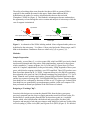
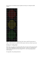
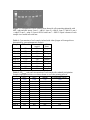
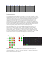
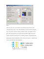
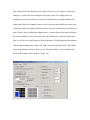
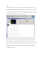
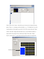
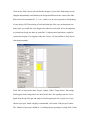
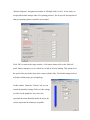
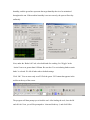
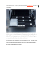
DNA microarrays: How to Make Your Own “Teaching Chips”
Spring, 2005. Davidson College.
Amore, A., Bossie, S., Citrin, M., Cobain, E., McDonald, M., Solé, M., Wilson, E.,
Choi, D., Oldham, E., Pierce, D. and Campbell, A.M.
ABSTRACT
DNA microarrays are an important tool in the fast-growing field of genomics. The
purpose of this investigation was two-fold. First, we learned to design and print DNA
microarrays, identifying some of the areas in these processes which we found
problematic. Despite our results, it is likely that results using the method described here
will improve. Our second goal was to develop a “teaching chip” protocol to be used in
other undergraduate settings. This paper describes one way that microarrays could be
incorporated into undergraduate genomics courses.
INTRODUCTION
DNA microarrays are becoming increasingly prevalent because this technology provides
investigators the opportunity to explore simultaneously the interactions among all genes
in an organism’s genome. Integrating comprehensive genomic research opportunities into
undergraduate education will facilitate advancement of the field of genomics, thus
broadening the potential medical applications of microarray technology. The pedagogical
value of this type of investigation is tremendous. Students gain experience designing and
implementing original experiments in addition to improving their understanding of the
principles underlying the creation and analysis of microarrays. As students become
confident with their abilities to explore microarray technology, they will develop a
comprehension that will rapidly escalate the utility of similar methodologies. For
example, pharmacogenomics examines how a patient’s genetic makeup affects his or her
response to a therapeutic drug regimen; an explosion of interest in this field would
positively affect an incredible number of patients.
A basic introduction to microarrays is available at the following web address:
http://www.ncbi.nlm.nih.gov/About/primer/microarrays.html (Microarrays, 2004).
Further conceptual information, including a description of the history and potential of
“The Microarray Revolution,” is presented in an article from Biochemistry and Molecular
Biology Education by Brewster (2004). Complementary DNA base pairing permits the
target/probe hybridization, which is the foundation of microarray technology. The
essential steps to this process are as follows: grow cells, isolate and extract RNA, convert
mRNA into cDNA, hybridize with Cy3 and Cy5 tagged probes, scan chip to measure
fluorescence intensity, analyze data to determine repression and induction patterns from
image profiles. For an animated overview of DNA microarray methodology, please refer
to the following website: http://www.bio.davidson.edu/Courses/genomics/chip/chip.html
(Campbell 2001).
The utility of teaching chips stems from the fact that no RNA or genomic DNA is
required for the methods presented in this paper. Rather than traditional RNA
hybridization, the probes we used are oligonucleotides that are detected with
Genisphere's 3DNA kit (Figure 1). This method is advantageous because students have
the opportunity to learn through the active creation and analysis of microarrays while the
cost of reagents is minimized.
Cy5 dendrimer
Cy3 dendrimer
5’
31mer capture sequence
5’
30mer oligo probe
500mer target
3’
31mer capture sequence
30mer oligo probe
3’
500mer target
Figure 1: A schematic of the 3DNA labeling method. 61mer oligonucleotide probes are
hybridized to the microarray. 30 of these 61 base pairs bind to the 500mer target, and 31
bind to the dendrimer. Dendrimers fluoresce either red (Cy5) or green (Cy3).
Methods:
Sample Preparation:
In this study, we used three S. cerevisiae genes (idh1, mhp2 and SHY) previously cloned
into bacterial plasmids and 61bp probes with complementary sequences to these genes
which contained a 5’ capture sequence, the Cy5 (red) and Cy3 (green) dyes (D. Pierce
and A.M. Campbell, unpublished). In the previous study, 500bp fragments of these yeast
genes, which had no sequence similarity, were PCR amplified. These PCR products were
then cloned into plasmid pCR 2.1-TOPO. Competent bacterial cells (JM109) containing
these plasmids were grown in 50mL LB Broth containing 50µl Ampicillin at 37°C for 16
hours. Plasmids were isolated using both the Qiagen HiSpeed Plasmid Purification Kit
and the less expensive Promega Pure Yield Plasmid Midi Prep System. Plasmid isolation
from both kits was confirmed by detection of DNA on a 0.7% agarose gel. Isolated DNA
from both kits was quantified by spectrophotometry and the yields were compared. We
then performed an ethanol precipitation of the DNA that was isolated.
Designing a “Teaching Chip”:
Our aim in this design was to orient the plasmid DNA from the three yeast genes
previously prepared onto the chip in a simple pattern that would yield clear results. We
decided that we would spot the plasmid DNA for these three genes in a “stoplight”
pattern, which, after hybridization with both red and green probes for these gene
sequences and merging of red and green images using MagicTool software would yield a
red circle (mhp), a yellow circle (idh1) and a green circle (SHY) (Figure 2). We decided
that in the space surrounding the genes printed on the chip we would print a buffer
solution.
Figure 2: Stoplight design using mhp (red), idh1 (yellow) and SHY (green) genes as
targets. Buffer solution was printed in all black squares that do not contain a gene name.
Printing the “Teaching Chip”:
DNA chips were printed on CSA amino slides (CEL Associates) in the pattern described
above using the BioRobotics MicroGrid II Compact. A total of 20_l of the DNA for
each gene was pipetted into the microwell plate in a 1:1 ratio with spotting solution
before printing.
See Appendix A for printing instructions.
Post-Printing Processing:
After printing, slides were crosslinked by UV light for three minutes using a DNA
transfer lamp from Fotodyne.
Pre–Hybridization Wash:
See appendix B
Hybridization Procedure:
See appendix C
Scanning Analysis:
Slides were scanned using an arrayWoRx escanner from Applied Precision.
Results and Discussion:
Sample Preparation:
We isolated plasmid DNA using both the Qiagen HiSpeed Midi Prep Kit and the
Promega Pure Yield Plasmid Midi Prep System. We ran all samples on a 0.7% agarose
gel to confirm that DNA had been recovered. The results from the gel indicated that both
kits did recover plasmid DNA in approximately equal amounts (Figure 3). In order to
compare the DNA yields achieved by both kits, we conducted a spectrophotometric
analysis to determine the concentration of DNA in each sample (Table 1). Both kits
produced similar DNA yields, indicating that they are equally as efficient despite the
difference in price of the two products. We did find that one Promega sample (idh1 #3)
had an unusually high yield however, we believed this to be due to the high protein
content in the sample (Table 1).
Although both kits were able to produce comparable yields, we found the Qiagen kit to
be most user friendly. Although the Qiagen kit is more expensive, there were very few
materials necessary to complete the plasmid isolation outside of what was provided in the
kit, whereas the Promega kit required several centrifugation steps that were often
cumbersome. After ethanol precipitation of these samples, we chose the one sample of
each gene with an OD260/280 ratio closest to 1.8 and a high concentration of DNA when
compared to the other samples of the same gene to use for printing our chips (Table 2).
Figure 3: Confirmation of DNA isolation from bacterial cells containing plasmids with
SHY, mhp and idh1 inserts. Lane 1 = idh1#1, Lane #2 = idh1#2, Lane 3 = idh1#3, Lane 4
= mhp#2, Lane 5 = mhp #3, Lane 6 SHY#1 and Lane 7 = SHY#2. Equal volumes of each
sample were loaded into each lane.
Table 1: Concentration of each sample isolated with either Qiagen or Promega kits as
determined by spectrophotometric analysis.
Sample
OD 260/280
Concentration
Kit
(µg/ml)
Name
idh1 #1
1.76
370
Qiagen
idh1 #2
1.76
440
Qiagen
idh1 #3
1.32
790
Promega
mhp #1
1.02
420
Qiagen
mhp #2
1.375
330
Qiagen
mhp #3
1.82
200
Promega
SHY #1
1.81
290
Qiagen
SHY #2
1.83
220
Promega
SHY #3
1.71
290
Qiagen
Table 2: OD260/280 ratio and concentration of each sample after ethanol precipitation.
Samples highlighted in blue were those chosen to use in the printing process.
Idh1 1a
Idh1 1b
Idh1 2a
Idh1 2b
Idh1 3a
Idh1 3b
OD260
0.360
0.046
0.015
0.266
0.353
0.512
OD280
0.220
0.046
0.017
0.164
0.247
0.375
260/280
1.64
1.00
0.88
1.64
1.43
1.37
Concentration (ug/mL)
7.20
0.92
0.30
5.32
7.06
10.24
Mhp 1a
Mhp 1b
Mhp 2a
Mhp 2b
Mhp 3a
Mhp 3b
0.183
0.528
0.305
N/A
0.399
N/A
0.105
0.303
0.171
N/A
0.285
N/A
1.74
1.74
1.78
N/A
1.40
N/A
3.66
10.56
6.10
N/A
7.98
N/A
SHY 1a
SHY 1b
SHY 2a
SHY 2b
SHY 3a
SHY 3b
0.356
0.340
0.200
N/A
0.327
0.282
0.208
0.194
0.135
N/A
0.243
0.177
1.71
1.75
1.48
N/A
1.35
1.59
7.12
6.80
4.00
N/A
6.54
5.64
Printing and Analysis:
After attempting the printing protocol several times, we were unable to produce a visible
stoplight pattern on any of our slides. Initially, there were several factors that we believed
contributed to this outcome. First, we recognized during the printing procedure that our
robot was not properly calibrated. However, after recalibration of the robot we still
encountered several difficulties. We also recognized that a probable source of error
included our failure to combine spotting solution in a 1:1 ratio with DNA sample in the
microwells before printing. Many of our initial scans revealed that our spots had dried up,
leaving very little sample on the slide for the probe to detect (data not shown). Once this
error was recognized, spotting solution was used in all subsequent trials.
After correcting these errors, we were still unable to obtain positive results (i.e. no
fluorescence was detected by the scanner). In order to further investigate probable
sources of error, we constructed a test slide that was hand spotted using 0.5_l of each
plasmid sample (120ng/_l and 240ng/_l), each oligo (provided by Sigma Proligo) and
two positive controls (provided by Genisphere) (Figure 4A). Once again, we were unable
to detect fluorescence on any spots other than the positive controls (Figure 4B).
A
B
Figure 4: Test Slide Design and Results. A: Anticipated results if all reagents were
functioning properly. O = oligo, RT = Reverse Transcript, C = control. B: Only the two
positive controls fluoresced as expected
Based upon these results we suspected that the capture sequence on the oligos used were
not complementary to the dendrimer sequences, thus not allowing binding to occur. We
determined that these sequences were in fact not complementary and thus, ordered new
oligos with the correct capture sequence (Table 3).
Table 3: Correct capture sequences for Cy3 and Cy5 dendrimers
Cy3
5’ TTC TCG TGT TCC GTT TGT ACT CTA AGG TGG A 3’
Cy5
5’ ATT GCC TTG TAA GCG ATG TGA TTC TAT TGG A 3’
Once the oligos with the correct capture sequence were obtained, we were able to obtain
positive results (Figure 5). Despite the many other sources of error discussed previously,
this mistake was by far the most significant. As a next step, the results obtained should
be analyzed using MagicTool® in order to quantify the level of fluorescence. Also,
optimization of the Cy5:Cy3 ratios needed to increase the fluorescence of Cy5 should be
completed, as our Cy5 signal was a bit weak.
Figure 5: Results obtained using oligos with the correct capture
sequence (Table 3). Note the appearance of the stoplight pattern.
We believe this protocol will be a useful teaching tool in the
undergraduate laboratory setting for students who have been
introduced to these techniques previously in the classroom. This
protocol gives undergraduate students the freedom to design their
own custom “teaching chips” and bridges the knowledge gap between
understanding the methodology and the actual practice of the
technique. With this basis, it is likely that undergraduate students will
be able to undertake more complex DNA microarray experiments
which may otherwise only be considered feasible in a graduate
setting.
Appendix A:
Modified Protocol for Cleaning the Pins
1. Soak pins in 50mM KOH for 5 minutes, careful not to let pin holder touch the
liquid (aluminum will get corroded).
2. Rinse pins in dH2O by wiggling in cup for ~5 seconds twice (in 2 separate
containers) to wash away excess salt.
3. Sonicate for 30 minutes to 1 hour with enough distilled water to fill basin within
an inch of the rim.
4. Soak in 90-95% EtOH for 30 minutes to 1 hour.
5. Let pins dry by hanging above EtOH for at least 5 minutes and not too much
longer (dust).
10 minutes + 1 hour + 1 hour +10 minutes = 2 hours and 20 minutes
Notes:
•Never let pin tips touch bottom of any container.
•It’s important to let pins dry before running the printer: washes may not be sufficient to
get EtOH off.
•30 minutes may be sufficient as a minimum for sonicate/soak, but the longer they do
each, the better they perform.
•Always wear powder-free gloves when handling the pin tool.
•Always clean pins before a major run. Once the pin tool has been placed back in its
polyethylene holder, it must be cleaned carefully in order to work.
Robot information:
Username: chippers
Password: spotters
ArrayWoRx information:
Username: awuser
Password: serca2a
Designing the printing pattern
Before you begin, you must decide on a printing pattern that establishes the orientation of
the spots on your chip. We designed a pattern that mimicked a stoplight using three
Mhp Mhp Mhp
Mhp Mhp Mhp Mhp Mhp
Mhp Mhp Mhp Mhp Mhp Mhp Mhp
different genes (idh1, mhp, and SHY). Asymmetric designs are best
so you can orient your slide after scanning.
Mhp Mhp Mhp Mhp Mhp Mhp Mhp
Mhp Mhp Mhp Mhp Mhp Mhp Mhp
It was helpful to use the cells of an Excel spreadsheet to plan the
Mhp Mhp Mhp Mhp Mhp
Mhp Mhp Mhp
idh1 idh1 idh1
idh1 idh1 idh1 idh1 idh1
idh1 idh1 idh1 idh1 idh1 idh1 idh1
idh1 idh1 idh1 idh1 idh1 idh1 idh1
idh1 idh1 idh1 idh1 idh1 idh1 idh1
idh1 idh1 idh1 idh1 idh1
spotting pattern. On your first attempt, it is best to choose a simple
design to establish a basic level of understanding. The key to a
simple design is a clear pattern while limiting the number of genes
used. Be sure when you choose your genes and probes, you are
idh1 idh1 idh1
aware of any partner-probe interactions, i.e. one probe with the
SHY SHY SHY
SHY SHY SHY SHY SHY
capacity to bind multiple genes (See D. Pierce, 2003).
SHY SHY SHY SHY SHY SHY SHY
SHY SHY SHY SHY SHY SHY SHY
SHY SHY SHY SHY SHY SHY SHY
SHY SHY SHY SHY SHY
SHY SHY SHY
Figure 1. Above is the design for our stoplight.
The red, yellow and green colors were generated
using the appropriate ratios of Cy3:Cy5.
Preparing the Robot
When not in use, be sure to keep the lid of the robot closed. It is best if the machine is
not in direct sunlight: be sure the blinds are closed, as this can alter humidity and
temperature beyond the control of the robot. First, the main power unit should be filled
with 6 Liters of de-ionized water. The bottle in the humidification control unit also needs
to be filled with de-ionized water to use the climate control system.
The white trays known as wash baths 1 & 2 should be filled with de-ionized water for
washing the pins. There are two slide trays in the robot. Be sure all holes on the slide
tray(s) you are using are covered, as this is necessary for creating a vacuum that will hold
the slides in place. If you are not using all slide slots in your study, you can cover the
extra holes on the tray by placing spare slides horizontally (see Fig. 2 on page 5).
Sample Preparation
Once a design has been decided upon, you must consider how the DNA samples will be
placed in the robot. The machine can hold samples in either a 96-well plate or a 384-well
plate. Although slides in most experiments will not require 384 separate samples, the use
of a 384-well plate is highly recommended. This is due to the fact that the smaller surface
area of the wells in the 384-well plate decreases volume of DNA needed and the amount
of evaporation. Next it will be necessary to determine how many samples you will need
to print your slide. In our design, we filled 3 wells with sample DNA plus spotting
solution in a 1:1 ratio and 3 wells with buffer solution (1X TE). Each well in use should
contain 10 to 25µl of sample; in our investigation, we used 20µl of sample per well.
Software
To begin your journey into microarray printing, first turn on your robot by switching on
the main power unit (MPU), followed by the humidification control unit (HCU).
Figure 2. The robot and its components: Main Power Unit (MPU), Humidification Control Unit (HCU).
It is now time to explore the wonderful world of your TAS Application Suite. Once the
program is opened, click on ‘New Microarray’ under the ‘File’ menu. The screen should
appear like this:
Options:
Under the options tab, you will define your well plate size (under ‘group’) and the pin
configuration (under ‘tool’). ‘Spots per source visit’ represents the number of times each
pin will touch the slides before returning to the 384-well plate (called the source). This
number should not exceed 30 to ensure the pin does not run out of sample. Under ‘wash
frequency’ you should choose ‘wash before new source visit,’ which ensures that no
sample mixing of DNA occurs. Next, click on the ‘Source’ tab.
Source:
Under the ‘Source’ tab, you will define where and how the pins will print. Under
‘Microplate Group’ choose ‘Classic Plate Definitions’. Be sure that under ‘Microplate
Type’ your specific well plate is selected. ‘Number of Plates’ is the number of source
plates. This option should be set at one since the MicroGridII Compact only has the
capacity to hold one microwell plate. The ‘Number of Samples’ is dependent upon the
printing pattern and pin configuration you have chosen. In our study, we wanted to print
from six wells in the following configuration:
Figure 3. Sample placement in the 384-well plate.
We printed from this sample configuration using 3 pins. A 3x1 pin configuration is not a
program option; therefore, we utilized the 3x2 pin configuration without loading the
second column of pins into the tool.
Figure 4. Robot arm and pin arrangement.
When a 3x2 pin configuration is chosen, the software assumes that 6 samples are present
in the source in a corresponding 3x2 configuration, filling wells A1-A3 and B1-B3.
When the ‘Number of samples’ tab is changed to 12, the software assumes that DNA
samples occupy wells A1-A3, B1-B3, C1-C3, and D1-D3. The software is then able to
obtain sample from wells A1-A3 and B1-B3 in one source visit, and sample from wells
C1-C3 and D1-D3 in a second source visit. In order to print our design, we set the sample
number at 12, loading our samples into wells A1-A3 and C1-C3. With this setup, we
were able to utilize a 3x2 pin configuration with only 3 pins and 6 true samples. ‘Last
plate’ defines how many different wells each pin will visit. For example, a 6-pin setup
making two visits to the microwell plate will require a total of 12 sample wells. Pay
attention to the text in this box; green means excellent (source visits and available tool
spots match), black is acceptable (source visits are less than the available tool spots), and
red indicates that a run cannot be initiated (source visits are greater than the available tool
spots). Under ‘Source loading into adapter plates’ you must choose how many well plates
the robot will hold at a time. Once again, this robot holds only 1 well plate. On the right
side, you will see an overall picture of the slide positions. If slides appear red the problem
must be addressed under the ‘Target’ tab. Under ‘Source action’ choose the ‘Dip’ option
when using split pins (which is what we use). ‘Prompt for plates’ is not available in the
MicrogridII Compact. Next, open the ‘Target’ tab.
Target:
Options under the ‘Target’ tab are very project specific. We will guide you on our
journey and try to explain the general logic (or lack thereof) of the software. Under the
‘Tool array definition’ you must click on the ‘Edit pattern’ button to inform the software
of the design you previously created (e.g. the spotlight).
First enter the values for the size of the grid that each pin will print. Each numbered
square represents one spot on the slide. The numbers in the boxes correspond to the
positions of the samples in the 384-microwell plate. When you click on the yellow spots
in the black box that appears at the top of the screen, the well plate coordinates are
displayed as seen below:
Under ‘Format’ click ‘Custom,’ as this allows you to create your own unique microarray
pattern. Choose n = x (entering your desired number, i.e. n = 2 for duplicates) if you wish
to print replicates of each sample on your slide. Click ‘OK’ to return to the main ‘Target’
window. Next under ‘Adapter Plate and Slide Layout,’ you will define the number of
targets (slides) to be printed. Click on ‘Edit Layout’ button. Then, under ‘Adapter
Layout’ you must select 27 vertical slides from the pull down menu. See image below:
384-Microwell Plate
Click on the ‘Slide Layout’ tab to define the margins of your slide. Each margin can be
changed independently and ultimately the design should be near the center of the slide.
Each colored area (numbered 1, 2, 3, etc.; yellow 1 in our case) represents a full printing
of your design, NOT the printing of each individual pin. Here you can determine how
many times you would like your design to be printed on each slide. In our investigation,
we printed our design one time on each slide. To adjust pattern replication, expand or
contract the margins. If red appears under the ‘Source’ tab, the problem is likely due to
your margin settings.
Click ‘OK’ to return to the main ‘Target’ window. Under ‘Target Action,’ the settings
which appear in the image above are ideal for the robot. Pre-spotting removes excess
liquid from the tip of the pin and ensures all subsequent spots are of equal size. If you
choose to pre-spot, which is highly recommended, click on the ‘Edit pre-spot’ button.
The ‘Number of pre-spots’ should be 1, confining the pre-spotting to a single slide. Under
‘Historical Options’, designate the number of ‘Multiple strikes’ to be 5. In our study, we
accepted the default settings under ‘Pre-spotting protocol’, but for specific descriptions of
other pre-spotting options consult the user manual.
Click ‘OK’ to return to the target window. A left mouse button click on the ‘Edit soft
touch’ button, transports you to a whole new world of decision making. This option slows
the speed of the pins before they make contact with the slide. The default settings worked
well and resulted proper spot morphology.
In this window, Under the ‘Climate’ tab, you can
control the humidity settings. Below are the settings
we chose. In the graph box, the yellow line
represents the actual humidity inside the robot, the
red line represents the minimum acceptable
humidity, and the green line represents the target humidity that is to be maintained
throughout the run. If the machine humidity is not set correctly, the spots will not dry
uniformly.
Next, under the ‘Baths 1&2’ tab, select both baths for washing. Set ‘Wiggle’ in the
‘Action’ box to no greater than 0.200mm. Be sure that ‘Use recirculating baths as static
baths’ is selected. We left all other tabs at default settings.
Click ‘OK.’ You are now ready to roll! Click the green ‘GO’ button that appears in the
tool bar at the top of the screen.
The program will then prompt you to load the tool. After loading the tool, close the lid
and click ok. Next, you will be prompted to ‘clean and load tray 1, and click OK to
switch on the vacuum.’ Be sure to push slides to the bottom (closest to you) left corner of
each slide slot.
Figure 5. Tray 1 setup with slides covering holes that create the vacuum.
After the vacuum is activated, the program will prompt you to ‘check that the slides are
held well. Check this by trying to move a slide and click ‘OK.’ The robot will begin its
run automatically. Sit back and relax until the run is finished.
Do not click the ‘Stop’ button unless you wish to terminate your run. The ‘Pause’ button
allows you to halt the program temporarily so that you can make minor adjustments to
the program before continuing your journey.
Appendix B: Pre-hybridization Wash
1. Wash the slides in 0.1% SDS for 2 min. (at RT)
2. Repeat step 1
3. Wash the slides in dH2O for 2 min. (at RT)
4. Boil the slides in H2O for 2.5 min.
5. Place the slides in 95% ethanol for 1 min. (at RT)
6. Spin at 1600 rpm for 2 min (or spray with pressurized CO2)
Appendix C:
1. Resuspend the oligos to a final concentration of 1ng/µl.
2. Vortex 25 µL of Buffer #6 (Genisphere®), 4 µL of each oligo, 1 µL calf thymus DNA
(1 ng/µL) and heat at 80°C for 10 min. This is the hybridization mixture.
Table 1: Oligonucleotide Probes With Corrected Capture Sequence (Not Bolded)
Cy3 SHY
5’ TTC TCG TGT TCC GTT TGT ACT CTA AGG TGG A
GCTGTAAACGGAACGCAAGCTGTTGATAAT 3’
Cy3 idh1
5’ TTC TCG TGT TCC GTT TGT ACT CTA AGG TGG A
GAACATGAATCCGTCCCTGGTGTAGTGGAA 3’
Cy3 Mhp
5’ TTC TCG TGT TCC GTT TGT ACT CTA AGG TGG A
AGTGATACCAACGGTACGAACGCAGATGAT 3’
Cy5 SHY
5’ ATT GCC TTG TAA GCG ATG TGA TTC TAT TGG A
GCTGTAAACGGAACGCAAGCTGTTGATAAT 3’
Cy5 idh1
5’ ATT GCC TTG TAA GCG ATG TGA TTC TAT TGG A
GAACATGAATCCGTCCCTGGTGTAGTGGAA 3’
Cy5 Mhp
5’ ATT GCC TTG TAA GCG ATG TGA TTC TAT TGG A
AGTGATACCAACGGTACGAACGCAGATGAT 3’
Table 2: Oligo ratios used.
Concentration (ng/_l)
Cy3 SHY
2620
Cy3 idh1
2380
Cy3 Mhp
1730
Cy5 SHY
2030
Cy5 idh1
3050
Cy5 Mhp
3150
3. In a test tube mix together the volume of hybridization mixture needed of each probe
in the appropriate ratios. See above (Table 3) for an example for our stoplight design.
4. Pipet 10µl of mixture onto slides under glass coverslip and incubate prepared slides at
42°C overnight, 12-18 hours
5. Wash slides in a Coplin jar with 2X SSC/ 0.2% SDS for 15 min. at 37°C
6. 2X SSC for 10 min. at room temperature
7. 0.2X SSC for 10 min. at room temperature
8. 95% EtOH for 1 min without air drying
9. Spin at 1600 rpm for 2 min.
10. Vortex 2.5 µL Cy3 dendrimer, 2.5 µL Cy5 dendrimer (or dH2O if only one
fluorophore is used) and 45 µL buffer #6; heat at 80°C for 10 min.
11. Incubate hybridized slides at 54°C for 2 hours
12. Using Coplin jars wrapped in aluminum foil, wash slides in 2X SSC/ 0.2% SDS for
15 min. at 54°C
13. 2X SSC for 10 min. at room temperature
14. 0.2X SSC for 10 min. at room temperature
15. 95% EtOH for 1 min without air drying
16. Spin at 1600 rpm for 2 min (or spray with pressurized CO2)
17. Keep slides in dark until ready to scan.