Download OLYMPUS Stream

User Manual
OLYMPUS Stream
IMAGE ANALYSIS SOFTWARE
Any copyrights relating to this manual shall belong to Olympus Soft Imaging
Solutions GmbH.
We at Olympus Soft Imaging Solutions GmbH have tried to make the information
contained in this manual as accurate and reliable as possible. Nevertheless,
Olympus Soft Imaging Solutions GmbH disclaims any warranty of any kind,
whether expressed or implied, as to any matter whatsoever relating to this
manual, including without limitation the merchantability or fitness for any
particular purpose. Olympus Soft Imaging Solutions GmbH will from time to time
revise the software described in this manual and reserves the right to make such
changes without obligation to notify the purchaser. In no event shall Olympus
Soft Imaging Solutions GmbH be liable for any indirect, special, incidental, or
consequential damages arising out of purchase or use of this manual or the
information contained herein.
No part of this document may be reproduced or transmitted in any form or by any
means, electronic or mechanical for any purpose, without the prior written
permission of Olympus Soft Imaging Solutions GmbH.
Adobe and Acrobat are trademarks of Adobe Systems Incorporated and be
registered in various countries.
© Olympus Soft Imaging Solutions GmbH
All rights reserved
Version 510_UMA_OlyStream19-Krishna_en_03_09July2013
Olympus Soft Imaging Solutions GmbH, Johann-Krane-Weg 39, D-48149 Münster,
Phone (+49)251/79800-0, Fax: (+49)251/79800-6060
Contents
1.
Before you start............................................................................................. 6
1.1.
Which documentation comes along with your software? ...............................................6
Online help for your software..........................................................................................6
1.2.
About your software........................................................................................................7
Main features of your software .......................................................................................7
2.
User interface ................................................................................................ 9
2.1.
Overview.........................................................................................................................9
2.2.
Layouts .........................................................................................................................11
2.3.
Document group ...........................................................................................................12
2.4.
Tool Windows ...............................................................................................................13
2.5.
Working with documents ..............................................................................................14
Saving documents ........................................................................................................14
Closing documents .......................................................................................................15
Opening documents .....................................................................................................15
Activating documents in the document group ..............................................................16
3.
4.
Configuring the system .............................................................................. 17
3.1.
Overview.......................................................................................................................17
3.2.
Configuring the system.................................................................................................18
Acquiring images ........................................................................................ 21
4.1.
Acquiring a single image ..............................................................................................21
4.2.
HDR images .................................................................................................................22
Acquiring an HDR image with an automatically set exposure range ...........................23
Acquiring more HDR images without setting the exposure range anew ......................24
4.3.
Acquiring movies and time stacks ................................................................................25
Recording a movie........................................................................................................25
Acquiring a time stack ..................................................................................................26
4.4.
Acquiring a Z-stack.......................................................................................................28
Acquiring a Z-stack.......................................................................................................28
4.5.
Acquiring an EFI image ................................................................................................29
Acquiring an EFI image without a motorized Z-drive....................................................30
4.6.
Creating stitched images ..............................................................................................34
Acquiring a stitched image without a motorized XY-stage (Manual MIA) ....................34
Acquiring a stitched image with a motorized XY-stage (XY-Positions / MIA) ..............38
Acquiring a stitched image with extended depth of focus ............................................41
Automatically acquiring several stitched images..........................................................42
Combining individual images into a stitched image......................................................43
5.
6.
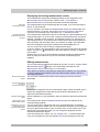
Processing images...................................................................................... 45
5.1.
Commenting images.....................................................................................................45
5.2.
Processing images .......................................................................................................45
Measuring images ....................................................................................... 47
6.1.
Overview.......................................................................................................................47
6.2.
Measuring images ........................................................................................................50
Measuring image objects interactively .........................................................................50
Outputting various measurement parameters ..............................................................52
Measuring several images............................................................................................54
Measuring heights ........................................................................................................55
6.3.
Measuring welding seams ............................................................................................58
Measuring a throat thickness........................................................................................58
Performing an asymmetry measurement .....................................................................62
7.
Performing a materials science analysis .................................................. 65
7.1.
Tool window - Materials Solutions ................................................................................65
Starting an analysis process.........................................................................................66
Selecting the image source ..........................................................................................67
Setting the stage path...................................................................................................69
7.2.
Chart comparison .........................................................................................................76
Performing a chart comparison ....................................................................................77
7.3.
Grains Intercept ............................................................................................................80
Settings for the intercept analysis.................................................................................81
Performing an intercept analysis ..................................................................................82
7.4.
Grains Planimetric ........................................................................................................86
Settings for the planimetric analysis.............................................................................87
7.5.
Layer Thickness............................................................................................................91
Settings for layer thickness measurements..................................................................93
Performing an automatic layer thickness measurement ..............................................94
Performing a layer thickness measurement with the magic wand (closed layer) ........97
Performing a manual layer thickness measurement ..................................................101
7.6.
Cast Iron Analysis.......................................................................................................104
Performing a cast iron analysis (unetched sample) ...................................................106
Performing a cast iron analysis (etched sample) .......................................................110
7.7.
Inclusions Worst Field ................................................................................................113
Performing an inclusions worst field analysis.............................................................114
Editing inclusions........................................................................................................116
7.8.
Throwing Power..........................................................................................................119
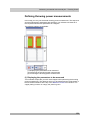
Defining throwing power measurements ....................................................................121
Performing a throwing power measurement ..............................................................123
7.9.
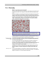
Porosity.......................................................................................................................128
Thresholds for porosity measurements ......................................................................130
Counting conditions for porosity measurements ........................................................132
Performing a porosity measurement ..........................................................................134
7.10. Phase analysis............................................................................................................138
Performing a phase analysis ......................................................................................141
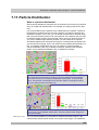
7.11. Particle Distribution.....................................................................................................145
Measuring the particle distribution..............................................................................147
7.12. Coating Thickness ......................................................................................................153
Measuring the coating thickness ................................................................................154
8.
Creating reports ........................................................................................ 158
8.1.
Overview.....................................................................................................................158
8.2.
Working with the report composer..............................................................................160
8.3.
Working with the Olympus MS-Office add-in..............................................................164
Creating and editing a new template..........................................................................165
Editing a report ...........................................................................................................167
Working with detail zooms..........................................................................................172
Before you start – Which documentation comes along with your software?
1.
Before you start
1.1. Which documentation comes along with
your software?
The documentation for your software consists of several parts: the installation
manual, the online help, and PDF manuals which were installed together with
your software.
Where do you find
which information?
A quick setup guide describing the software activation is delivered with your
software.
On the setup-DVD, several PDF manuals are provided.



In the installation manual, you can find the system requirements.
Additionally, you can find out how to install and configure your software.
In the user manual, you will find both an introduction to the product and
an explanation of the user interface. By using the extensive step-by-step
instructions you can quickly learn the most important procedures for
using this software.
The database is explained in its own user manual.
In the online help, you can find detailed help for all elements of your software. An
individual help topic is available for every command, every toolbar, every tool
window and every dialog box.
New users are advised to use the manual to introduce themselves to the product
and to use the online help for more detailed questions at a later date.
Writing convention
used in the
documentation
Example images that
are automatically
installed
In this documentation, the term "your software" will be used for OLYMPUS
Stream.
During the installation of your software some sample images have been installed,
too. These example images might be of help to you when you familiarize yourself
with your software.
00018
Online help for your software
In the online help, you can find detailed help for all elements of your software. An
individual help topic is available for every command, every toolbar, every tool
window and every dialog box.
When you use the help mode, you'll have access to most online topics. As soon
as you use the Context help command, you will find yourself in the help mode. In
the help mode, a question mark will be attached to the mouse pointer. Then you
will be able to call for help on almost all of your software's functions.
Switching to the help
mode
There are various ways of switching to the help mode.



Click the Context Help
button. You can find this button on the
Standard toolbar.
Use the Help > Context Help command.
Use the [Shift + F1] shortcut.
00087
6
Before you start – About your software
1.2. About your software
Note: Not every software package contains all of the features!
To support the different requirements on the software optimally, a variety of
packages are available for your software. The larger software packages contain
more features than the smaller packages. For example, the smaller packages
contain only restricted database functionality.
Some of the functions described are, therefore, of no relevance to users of
smaller packages.
Main features of your software
Acquiring images
You can use your system to acquire high resolution images of a sample in a few
steps. Your system is comprised of your software and the hardware, e.g.,
microscope and camera. During image acquisition, the data from the camera
which is mounted on your microscope will be read out and displayed on your
computer's monitor.
You can first examine the live-image and adjust it optimally. The live-image will
be constantly updated, i.e., when you, for example, move the stage to a different
position, the live-image will be changed accordingly. You can switch the liveimage on and off and acquire a photo of the parts of the sample that interest you.
When you do this, you will create a digital image that you can save and process
or analyze with a variety of your software's functions.
Acquiring and viewing
multi-dimensional
images
Acquiring an EFI image
Acquiring stitched
images
A multi-dimensional image is always made up of several frames. These have, for
example, been acquired at different times, or in different focus positions. With
your software you can, e.g., acquire a time stack or a Z-stack. For optimum
viewing of multi-dimensional images, use the separate navigation bar that is
shown directly in the image window when a multi-dimensional image is loaded.
With your software, you can acquire images which have a practically unlimited
depth of focus. These images are called EFI images. EFI is the abbreviation for
"Extended Focal Imaging". For the creation of an EFI image, the software
determines which of the pixels from the differently focused frames in a Z-stack
are the sharpest, and calculates an image that is sharply focused in all areas
from them.
When your system is equipped with a motorized XY-stage: Use the XY-Positions
/ MIA acquisition process to acquire a stitched image of a larger part of the
sample. MIA stands for Multiple Image Alignment. During the acquisition, this
acquisition process directly combines all of the images that are acquired, into a
stitched image, just like a puzzle.
When your system is not equipped with a motorized XY-stage: Use the Manual
MIA acquisition process and manually move the stage to have the different,
adjoining parts of the sample put on display one after the other. By using this
acquisition process directly during the acquisition, you combine all of the images
that are acquired into a stitched image, just like a puzzle.
Saving documents in a
database
You can insert not only images, but also documents which have another file
format into a database. That enables you to store all manner of data that belongs
together in one location. Search and filter functions make it quick and easy to
locate documents.
Images will, by default, be saved in the TIF or VSI file format. When you save an
acquired image in TIF format, a lot of important image information will be
automatically saved with it, for example, data concerning the camera used, the
exposure time, the resolution, the time of creation, and so on. You can later view
7
Before you start – About your software
this data again whenever you want, simply by opening the image with your
software. You do not need to collect this data separately.
A PDF manual for your database is installed together with your software.
Measuring images
You can make various measurements on images, and, e.g., measure the length
of a line, the perimeter of an ellipse or an angle in degrees. The measurement
objects will be displayed in the image's drawing layer, and can be faded in and
out. The measurement results will be shown in a sheet and can be differently
sorted by a click of your mouse. You can export measurement results, for
example, to the XLS format (for further editing in the MS-Excel application
program).
You can measure an image, or several images at the same time, according to
different material science analysis processes.
The Materials Solutions tool window works similarly to a software wizard. As
soon as you've started an analysis process you'll be guided step by step through
the measurement.
The following material science analysis processes are available:












Chart comparison
Grains Intercept
Grains Planimetric
Layer Thickness
Cast Iron Analysis
Inclusions Worst Field
Throwing Power
Porosity
Phase Analysis
Particle Distribution
Automatic Measurement
Coating Thickness
Processing images
You can process the acquired images and retroactively optimize the image
quality according to your requirements. Numerous filters and functions are
available for this purpose, e.g., various smoothing or sharpness filters, and
functions to optimize the contrast. As well as this, you can mirror the images and
also rotate them through an arbitrary number of degrees.
Analyzing images
automatically
With an automatic image analysis, your software searches for areas in an image
that have the same intensity, or color. All of the areas that have the same
intensity, or color will be assigned to a phase, and evaluated. This makes it
possible to automate typical measurement tasks. You can, for example,
determine the area ratios of the different phases in an image.
Creating reports
You can document the results of your work in a report. To do this, select the
required page templates and images in the Report Composer tool window, for
example, and generate an MS-Word report.
In case you want to insert images, workbooks or charts from your software into
new or existing MS-Word or MS-PowerPoint documents, use a special Olympus
add-in for this. With the help of this add-in, you can access all documents and
data that you created with your image analysis program from MS-Word or MSPowerPoint. You can apply different options to all the MS-Word or MSPowerPoint report's images, detail zooms, for example. It's sufficient for your
image analysis program to be open in the background.
Controlling the
microscope
You can control your microscope's motorized parts via the software. For
example, you can change an objective, load an ND filter, or open and close a
shutter, with your software. To make this communication function, the
components must not only be motorized, but also have been configured in the
software.
00017 15052013
8
User interface – Overview
2.
User interface
2.1. Overview
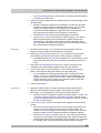
The graphical user interface determines your software's appearance. It specifies
which menus there are, how the individual functions can be called up, how and
where data, e.g. images, is displayed, and much more. Here, the basic elements
of the user interface are described.
Note: Your software's user interface can be adapted to suit the requirements of
individual users and tasks. You can, e.g., configure the toolbars, create new
layouts, or modify the document group in such a way that several images can be
displayed at the same time.
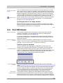
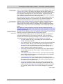
Appearance of the user
interface
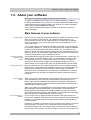
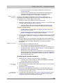
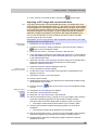
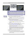
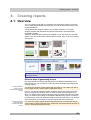
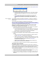
The illustration shows the schematic user interface with its basic elements.
(1) Menu bar
(2) Document group
(3) Toolbars
(4) Tool windows
(5) Status bar
(1) Menu bar
You can call up many commands by using the corresponding menu. Your
software's menu bar can be configured to suit your requirements. Use the Tools
> Customization > Start Customize Mode... command to add menus, modify, or
delete them.
You can find more information in the online help.
(2) Document group
The document group contains all loaded documents. These can be of all
supported document types.
When you start your software, the document group is empty. While you use your
software it gets filled - e.g., when you load or acquire images, or perform various
image processing operations to change the source image and create a new one.
9
User interface – Overview
(3) Toolbars
Commands you use frequently are linked to a button providing you with quick
and easy access to these functions. Please note, that there are many functions
which are only accessible via a toolbar, e.g., the drawing functions required for
annotating an image. Use the Tools > Customization > Start Customize Mode...
command to modify a toolbar's appearance to suit your requirements.
(4) Tool windows
Tool windows combine functions into groups. These may be very different
functions. For example, in the Properties tool window you will find all the
information available on the active document.
In contrast to dialog boxes, tool windows remain visible on the user interface as
long as they are switched on. That gives you access to the settings in the tool
windows at any time.
(5) Status bar
The status bar shows, e.g., a brief description of each function. Simply move the
mouse pointer over the command or button for this information.
You can also find additional information in the status bar.
00108
10
User interface – Layouts
2.2. Layouts
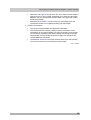
What is a layout?
Your software's user interface is to a great extent configurable, so that it can
easily be adapted to meet the requirements of individual users or of different
tasks. You can define a so-called "layout" that is suitable for the task on hand. A
"layout" is an arrangement of the control elements on your monitor that is optimal
for the task on hand. In any layout, only the software functions that are important
in respect to this layout will be available.
Example: The Camera Control tool window is only of importance when you
acquire images. When instead of that, you want to measure images, you don't
need that tool window.
That's why the "Acquisition" layout contains the Camera Control tool window,
whereas in the "Processing" layout it's hidden.
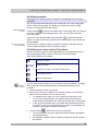
Which elements of the
user interface belong to
the layout?
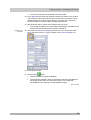
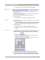
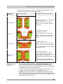
The illustration shows you the elements of the user interface that belong to the
layout. The layout saves the element's size and position, regardless of whether
they have been shown or hidden. When, for example, you have brought the
Windows toolbar into a layout, it will only be available for this one layout.
(1) Toolbars
(2) Tool windows
(3) Status bar
(4) Menu bar
Switching to a layout
Which predefined
layouts are there?
To switch backwards and forwards between different layouts, click on the righthand side in the menu bar on the name of the layout you want, or use the View >
Layout command.
For important tasks several layouts have already been defined. The following
layouts are available:




Work with a database ("Database" layout )
Acquire images ("Acquisition" layout)
View and process images ("Processing" layout)
Generate a report ("Reporting" layout )
In contrast to your own layouts, predefined layouts can't be deleted. Therefore,
you can always restore a predefined layout back to its originally defined form. To
do this, select the predefined layout, and use the View > Layout > Reset Current
Layout command.
00013
11
User interface – Document group
2.3. Document group
The document group contains all loaded documents. These can be of all
supported document types.
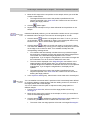
Appearance of the
document group
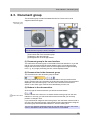
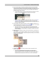
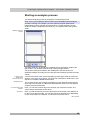
The illustration shows left, a schematic representation of a user interface. On the
right, the document group is shown enlarged.
(1) Document group in the user interface
(2) Document bar in the document group
(3) Buttons in the document bar
(4) Navigation bar in the image window
(1) Document group in the user interface
You will find the document group in the middle of the user interface. In it you will
find all of the documents that have been loaded, and of course also all of the
images that have been acquired. Also the live-image and the images resulting
from, e.g., any image processing function, will be displayed there.
(2) Document bar in the document group
The document bar is the document group's header.
For every loaded document, an individual field will be set up in the document
group. Click the name of a document in the document bar to have this document
displayed in the document group. The name of the active document will be
shown in color. Each type of document is identified by its own icon.
(3) Buttons in the document bar
At the top right of the document bar you will see several buttons.
Button with a hand
Click the button with a hand on it to extract the document group from the user
interface. In this way you will create a document window that you can freely
position or change in size.
If you would like to merge two document groups, click the button with the hand in
one of the two document groups. With the left mouse button depressed, drag the
document group with all the files loaded in it, onto an existing one.
You can only position document groups as you wish when you are in the expert
mode. In standard mode the button with the hand is not available.
12
User interface – Tool Windows
Arrow buttons
Button with a cross
The arrow buttons located at the top right of the document group are, to begin
with, inactive when you start your software. The arrow buttons will only become
active when you have loaded so many documents that all of their names can no
longer be displayed in the document group. Then you can click one of the two
arrows to make the fields with the document names scroll to the left or the right.
That will enable you to see the documents that were previously not shown.
Click the button with a cross to close the active document. If it has not yet been
saved, the Unsaved Documents dialog box will open. You can then decide
whether or not you still need the data.
(4) Navigation bar in the image window
Multi-dimensional images have their own navigation bar directly in the image
window. Use this navigation bar to determine how a multi-dimensional image is
to be displayed on your monitor, or to change this.
00139
2.4. Tool Windows
What is a tool window?
Tool windows combine functions into groups. These may be very different
functions. For example, in the Properties tool window you will find all the
information available on the active document.
In contrast to dialog boxes, tool windows keep visible on the user interface as
long as they are switched on. That gives you access to the settings in the tool
windows at any time.
Showing and hiding tool
windows
Which tool windows are shown by default depends on the layout you have
chosen. You can, at any time, make specific tool windows appear and disappear
manually. To do so, use the View > Tool Windows command.
Position of the tool windows
The user interface is to a large degree configurable. For this reason, tool
windows can be docked, freely positioned, or integrated in document groups.
Docked tool windows
Tool windows can be docked to the left or right of the document window, or
below it. To save space, several tool windows may lie on top of each other. They
are then arranged as tabs. In this case, activate the required tool window by
clicking the title of the corresponding tab below the window.
Freely positioned tool
windows
You can only position tool windows as you wish when you are in the expert
mode.
You can at any time float a tool window. The tool window then behaves exactly
the way a dialog box does. To release a tool window from its docked position,
click on its header with your left mouse button. Then, while keeping the left
mouse button depressed, drag the tool window to wherever you want it.
Saving the tool
window's position
Tool windows and their positions are saved together with the layout and are
available at the same position the next time you start your software. Resetting
the layout using the View > Layout > Reset Current Layout command will have
the result that only the tool windows that are defined by default will be displayed.
13
User interface – Working with documents
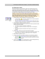
Buttons in the header
In the header of every tool window, you will find the three buttons Help, Auto
Hide and Close.
Click the Help button to open the online help for the tool window.
Click the Auto Hide button to minimize the tool window.
Click the Close button to hide the tool window. You can make it reappear at any
time, for example, with the View > Tool Windows command.
Context menu of the header
To open a context menu, rightclick a tool window's header. The context menu
can contain the Auto Hide and Transparency commands.
Additionally, the context menu contains a list of all of the tool windows that are
available. Every tool window is identified by its own icon. The icons of the
currently displayed tool windows will appear clicked. You can recognize this
status by the icon's background color.
Use this list to make tool windows appear.
00037
2.5. Working with documents
You can choose from a number of possibilities when you want to open, save, or
close documents. As a rule, these documents will be images. In addition, your
software supports some other document types. You will find a list of supported
documents in the online help.
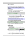
Saving documents
You should always save important documents immediately following their
acquisition. You can recognize documents that have not been saved by the star
icon after the document's name.
There are a number of ways in which you can save documents.
1. To save a single document, activate the document in the document group
and use the File > Save As... command.
2. Use the Documents tool window.
Select the desired document and use the Save command in the context
menu. For the selection of documents, the standard MS-Windows
conventions for multiple selection are valid.
3. Use the Gallery tool window.
Select the desired document and use the Save command in the context
menu. For the selection of documents, the standard MS-Windows
conventions for multiple selection are valid.
4. Save your documents in a database. That enables you to store all manner of
data that belongs together in one location. Search and filter functions make it
quick and easy to locate saved documents. Detailed information on inserting
documents into a database can be found in the online help.
Autosave and close
1. When you exit your software, all data that has not yet been saved will be
listed in the Unsaved Documents dialog box. This gives you the chance to
decide which document you still want to save.
2. With some acquisition processes, the acquired images will be automatically
saved after the acquisition has finished.
14
User interface – Working with documents
3. You can also configure your software in such a way that all images are saved
automatically after image acquisition. To do so, use the Acquisition Settings
> Saving dialog box.
Here, you can also configure your software in such a way that all images are
automatically saved in a database after the image acquisition.
Closing documents
There are a number of ways in which you can close documents.
1. Use the Documents tool window.
Select the desired documents and use the Close command in the context
menu. For the selection of documents, the standard MS-Windows
conventions for multiple selection are valid.
2. To close a single document, activate the document in the document group
and use the File > Close command. Alternatively, you can click the button
with the cross . You will find this button on the top right in the document
group.
3. Use the Gallery tool window.
Select the desired documents and use the Close command in the context
menu. For the selection of documents, the standard MS-Windows
conventions for multiple selection are valid.
Closing all documents
Closing a document
immediately
To close all loaded documents use the Close All command. You will find this
command in the File menu, and in both the Documents and the Gallery tool
window's context menu.
To close a document immediately without a query, close it with the [Shift] key
depressed. Data you have not saved will be lost.
Opening documents
There are a number of ways in which you can open or load documents.
1. Use the File > Open... command.
2. Use the File Explorer tool window.
To load a single image, double click on the image file in the File Explorer tool
window.
To load several images simultaneously, select the images and with the left
mouse button depressed, drag them into the document group. For the
selection of images the standard MS-Windows conventions for multiple
selection are valid.
3. Drag the document you want, directly out of the MS-Windows Explorer, onto
your software's document group.
4. To load documents from a database into the document group, use the
Database > Load Documents... command. You can find more information in
the online help.
Generating a test
image
If you want to get used to your software, then sometimes any image suffices to
try out a function.
Press [Ctrl + Shift + Alt + T] to generate a color test image.
With the [Ctrl + Alt + T] shortcut, you can generate a test image that is made up
of 256 gray values.
15
User interface – Working with documents
Activating documents in the document group
There are several ways to activate one of the documents that has been loaded
into the document group and thus display it on your monitor.
1. Use the Documents tool window. Click the desired document there.
2. Use the Gallery tool window. Click the desired document there.
3. Click the title of the desired document in the document group.
4. To open a list with all currently loaded documents, use the [Ctrl + Tab]
shortcut. Leftclick the document that you want to have displayed on your
monitor.
5. In the Window menu, you will find a list of all of the documents that have
been loaded. Select the document you want from this list.
Document group and
database
Please note that in the Database layout the document group will not be shown.
Select one of the other layouts, e.g., the Processing layout, to have the
document group displayed.
00143 08052012
16
Configuring the system – Overview
3.
Configuring the system
3.1. Overview
Why do you have to
configure the system?
After successfully installing your software you will need to first configure your
image analysis system, then calibrate it. Only when you have done this will you
have made the preparations that are necessary to ensure that you will be able to
acquire high quality images that are correctly calibrated. When you work with a
motorized microscope, you will also need to configure the existing hardware, to
enable the program to control the motorized parts of your microscope.
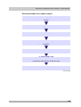
Process flow of the configuration
To set up your software, the following steps will be necessary:
Specifying which hardware is available
Configuring the interfaces
Configuring the specified hardware
Calibrating the system
Specifying which
hardware is available
Configuring the
interfaces
Configuring the
specified hardware
Calibrating the system
Your software has to know which hardware components your microscope is
equipped with. Only these hardware components can be configured and
subsequently controlled by the software. In the Acquire > Devices > Device List
dialog box, you select the hardware components that are available on your
microscope.
You can find more information on this dialog box in the online help.
Use the Acquire > Devices > Interfaces command, to configure the interfaces
between your microscope or other motorized components, and the PC on which
your software runs.
You can find more information on this dialog box in the online help.
Usually various different devices, such as a camera, a microscope and/or a
stage, will belong to your system. Use the Acquire > Devices > Device Settings...
dialog box to configure the connected devices so that they can be correctly
actuated by your software.
You can find more information on this dialog box in the online help.
When all of the hardware components have been registered with your software
and have been configured, the functioning of the system is already ensured.
However, it's only really easy to work with the system and to acquire top quality
images, when you have calibrated your software. The detailed information that
helps you to make optimal acquisitions, will then be available.
Your software offers a wizard that will help you while you go through the
individual calibration processes. Use the Acquire > Calibrations... command to
start the software wizard.
You can find more information on this dialog box in the online help.
17
Configuring the system – Configuring the system
About the system configuration
When do you have to
configure the system?
You will only need to completely configure and calibrate your system anew when
you have installed the software on your PC for the first time, and then start it.
When you later change the way your microscope is equipped, you will only need
to change the configuration of certain hardware components, and possibly also
recalibrate them.
Necessary user rights
for the system
configuration
To be able to configure the system, you have to be logged in to your software
with administrator or power user rights. If you have installed the software yourself
you will automatically have been assigned Administrator rights.
In contrast, other users who also wish to work with the software will only have
user rights as a Standard User. With these rights, the system configuration
cannot be changed or viewed, i.e., the Device List and Device Settings dialog
boxes cannot be opened.
For this reason, those users who did not themselves install the software, but who
are to be allowed to view or change the system configuration, have to be
assigned the necessary user rights. Use the Tools > User Rights... command to
open the User Rights dialog box. In it, select the required user, then click the
Properties... button.
You can find more information on user rights in the online help.
Switching off your
operating system's
hibernation mode
When you use the MS-Windows Vista operating system: Switch the hibernation
mode off.
To do so, click the Start button located at the bottom left of the operating
system's task bar.
Use the Control Panel command.
Open the System and Maintenance > Power Options > Change when the
computer sleeps window. Here, you can switch off your PC's hibernation mode.
00159
3.2. Configuring the system
In order to acquire correctly calibrated images, the software requires information
about your camera, the objectives and the microscope camera adaptor's
magnification. Set up your system with this in mind.
Preconditions
Your software is installed and the camera is connected to your PC. The camera
driver is installed in MS-Windows.
Specifying which hardware is available
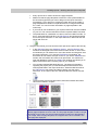
1. Start your software.
Setting up a new
hardware configuration
2. Use the Acquire > Devices > Device List... command.
3. Click the Create New Hardware Configuration

button.
The Create New Hardware Configuration dialog box will open.
4. Enter a name for the new hardware configuration in the Name field. It is a
good idea to choose a name combining the microscope and camera names,
for example, "BX51_DP25“.

Under this name, you can later reload this hardware configuration in the
Device Settings dialog box.
5. Select the Copy current hardware configuration option if you have previously
chosen your camera and microscope. Otherwise, choose the Empty
hardware configuration option.
6. Close the Create New Hardware Configuration dialog box with OK to return
to the Device List dialog box.
18
Configuring the system – Configuring the system
Defining a hardware
configuration

You will then find the new hardware configuration entered in the
Configuration field.

Once you have completely set up a new hardware configuration, all
entries from the Device List will be empty. You can now enter a
completely new definition for the hardware configuration.
Define the new hardware configuration in the Device List dialog box. A
description of this dialog box can be found in the online help. Begin with the
specifications for the camera and the microscope.
7. Select your camera (e.g. "DP25") from the Camera 1 list.
8. Select your microscope (e.g. "BX51") from the Frame list. If your microscope
isn't listed, select the Manual Microscope entry.

Once you have chosen a microscope, the options in the Device List
dialog box change. For some microscopes there are default settings .
Examples of default settings:

For the manual microscope BX51, the Manual Nosepiece entry from
theNosepiece list is preset.

For the manual stereo microscope SZX10, the Manual Nosepiece and
Manual Zoom/Magnification Changer entries are preset.
9. For some microscopes (such as IX71), you need to choose the port on which
your camera is mounted (e.g. Side (left)). You find the list to the right of the
camera list.
10. All other settings, such as nosepiece, observation filter wheel, shutter and
condensor are appropriately preset, independent of your microscope. Check
your settings and, if necessary, adjust them to suit your microscope
equipment.
Initializing your devices
11. Close the Device List dialog box with OK.

Your hardware configuration will be automatically saved.

You can return to the default configuration whenever you want to. To do
so, use the Acquire > Devices > Device Settings... command. Select the
Default entry in the Configuration list.

As soon as you close the Device List dialog box, your software will try to
set up the connection to the specified devices. You can see whether the
devices are able to be successfully controlled in the Acquire > Devices >
Device Settings device box.
Configuring the specified hardware
1. Use the Acquire > Devices > Device Settings... command.

In the tree view on the left side, you can find all hardware components
that you have chosen in the device list.
2. Select the Lightpath entry in the Sort by list.
Configuring your
camera
3. In the tree view on the left-hand side, expand the Camera > <camera name>
entry (e.g. "DP25“).
4. Select the Camera Adapter entry.
5. Select your camera adapter's magnification on the right-hand side of the
Magnification list. The magnification is imprinted on your camera adapter.
Common values are "1.00" or "0.63".
Configuring the
objective nosepiece
6. In the tree structure, either select the General > Manual Nosepiece entry (if
you have a manual microscope), or General > Nosepiece <Name of the
nosepiece> (if you have a motorized microscope).
19
Configuring the system – Configuring the system

On the right hand side of the dialog box, the current configuration of the
nosepiece will be displayed. When you configure the software for the first
time, the fields for the details referring to your objectives will be empty.
7. Choose the objectives which are currently fitted to the nosepiece from the
right-hand side of the Magnification lists. Start with the smallest magnification
and increase up through the higher magnifications. You can read the
magnification off of the objective.
8. Choose each corresponding objective from the Objective Type list. The type
is written on the objective.

In the Description field, a description of the objective will be suggested.
You may change the description of the objective in the Description field,
if you wish.
9. If the objectives don't use air as their refraction medium, select the immersion
medium from the Refraction Index list. In this case, you find an appropriate
label on the objective.
Configuring the mirror
turret
10. Select the General > <Name of the mirror turret> entry in the tree view.
11. Make a selection for every position, whether it is occupied or not. For
occupied positions, either select a filter or fluorescence cube being used from
the Filter list, or enter the name of your filter module.
12. Select the Free entry for positions that have been purposely left free to keep
the light path free of optical elements.
For example, where the mirror turret is concerned, it is especially important
that one position is kept free, in order not to impede the light path for the
transmitted light microscopy.
Finishing system
configuration
13. Close the Device Settings dialog box with OK.

In certain cases, you receive a message telling you to check the
calibrations. You can perform calibration now or later.
14. To have this toolbar displayed, use the View > Toolbars > Microscope
Control command.

The Microscope Control toolbar contains buttons with all of your
objectives with correct color codes.

For stereo microscopes or inverted microscopes, you find the zoom
factors in the list to the right of the objectives.
00156
20
Acquiring images – Acquiring a single image
4.
Acquiring images
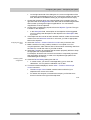
4.1. Acquiring a single image
You can use your software to acquire high resolution images in a very short
period of time. For your first acquisition you should carry out these instructions
step for step. Then, when you later make other acquisitions, you will notice that
for similar types of sample many of the settings you made for the first acquisition
can be adopted without change.
1. Switch to the "Acquisition" layout. To do this, use, e.g., the View > Layout >
Acquisition command.

You can find the Microscope Control (1) toolbar at the upper edge of the
user interface, right below the menu bar.
To the right of the document group, you can find the Camera Control (2)
tool window.
Selecting an objective
2. On the Microscope Control toolbar, click the button with the objective that
you use for the image acquisition.
Switching on the liveimage
3. In the Camera Control tool window, click the Live button.

The live-image (3) will now be shown in the document group.
4. Go to the required specimen position in the live-image.
Setting the image
quality
5. Bring the sample into focus. The Focus Indicator toolbar is there for you to
use when you are focusing on your sample.
6. Check the color reproduction. If necessary, carry out a white balance.
7. Check the exposure time. You can either use the automatic exposure time
function, or enter the exposure time manually.
8. Select the resolution you want.
Acquiring and saving
an image
9. In the Camera Control tool window, click the Snap button.

The acquired image will be shown in the document group.
10. Use the File > Save As... command to save the image. Use the
recommended TIF file format.
00027
21
Acquiring images – HDR images
4.2. HDR images
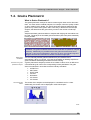
What are HDR images?
Under the microscope, certain samples (with very reflective metal surfaces, for
example) can have such strong differences in brightness that it is impossible to
find an exposure time that is suitable for all areas of the sample.
For such samples, an HDR image acquisition is recommended. HDR stands for
High Dynamic Range. Dynamic range relates to the capacity of cameras, or
image processing software, to display both the bright and the dark segments of
an image well.
Before acquiring an HDR image, the necessary exposure range needs to be
determined for the current sample. The exposure range is made up of a minimum
and maximum exposure time as well as several exposure times between them.
Several individual images are then taken of the sample with differing exposure
times, so that no image segment is left over or underexposed.
Your software then detects the best exposed pixels in each acquired individual
image and merges them into one new image. Under correctly defined acquisition
conditions, the HDR image will no longer contain any under or overexposed
image segments.
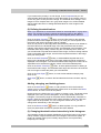
Just like with images acquired with Extended Focal Imaging (EFI image), an
HDR image is a rendered image containing information from several images.
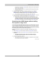
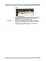
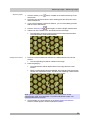
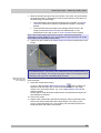
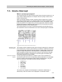
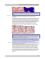
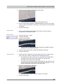
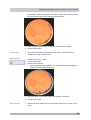
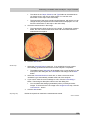
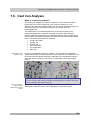
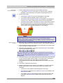
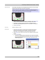
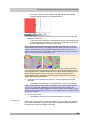
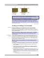
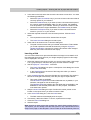
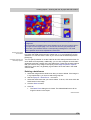
Here, you can see an image acquired of a very reflective metal surface. Example
1 shows an image which was not acquired using HDR. The reflective segments
of the surface are correctly exposed, whereas other segments are completely
underexposed. Example 2 shows an image which was acquired using HDR.
Without overexposing the reflective segments of the surface, now the structures
in the dark image segments, which were not recognizable before, are visible.
Determining the
exposure range
A recently determined exposure range will continue to be used for all HDR
images until you let your software determine the exposure range anew. It is
irrelevant whether the exposure range had been determined automatically or
manually.
If you are acquiring several images of the same or similar parts of a sample, you
don't need to determine the exposure range each time. If you change the sample
or adjust settings on the microscope, it is recommended to determine the
exposure range anew (either automatically or manually).
HDR images and
acquisition processes
HDR images and movie
recording
You can also insert an HDR image acquisition into an acquisition process, such
as during the acquisition of a time-lapse image or a Z-stack. The Process
Manager tool window informs you about the status of the HDR image acquisition.
If the Activate HDR check box is selected in the Camera control tool window, the
Process Manager tool window shows the Active entry in the HDR field. If the
check box is deselected, the Process Manager tool window shows the entry Off
in the HDR field.
It is not possible to record movies with HDR. Because of this, the Activate HDR
check box is ignored while the Movie recording check box is selected.
07510 04072011
22
Acquiring images – HDR images
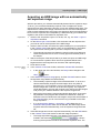
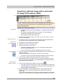
Acquiring an HDR image with an automatically
set exposure range
With this procedure, your software automatically determines the exposure range.
To do so, your camera automatically acquires a set of images with various
exposure times and measures the amount of over and underexposed pixels. The
exposure time continues to change until the amount of over and underexposed
pixels is within defined limits. At this point, the exposure range has been defined.
How much the exposure time is adjusted by is determined by your software with
regards to the minimum and maximum exposure time.
Preparations
1. Switch to the "Acquisition" layout. To do this, use, e.g., the View > Layout >
Acquisition command.
2. On the Microscope Control toolbar, click the button with the objective that
you want to use for the acquisition of the HDR image.
3. Switch to the live mode, and select the optimal settings for your acquisition,
in the Camera Control tool window. Carry out a white balance. Then select
an exposure time meaning that no part of the sample is overexposed.

The automatic exposure time detection uses this value as a basis and
raises the exposure time so as to correctly light even the dark parts of
the sample.
4. Search for the part of the sample which you want to acquire an HDR image
of. This should be a position which has such significant differences in
brightness that not all segments can be shown with optimal lighting.
5. Finish the live mode.
Acquiring an HDR
image
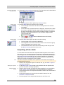
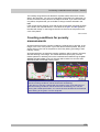
6. In the Camera Control tool window, select the Activate HDR check box.

In the upper part of the tool window, the Snap button changes to the
HDR
button.
7. In the Determine exposure range group, click the Automatic button to have
the exposure range determined automatically.

The necessary exposure range will now be determined. To do so, the
camera automatically acquires several images which only differ in
exposure time. This acquisition occurs in the background, which means
that the images are not shown in the document group. The exposure
range determined in this way will continue to be used for all HDR images
until you let your software determine the exposure range anew.

Determining the exposure range automatically takes about 30 seconds.
Pay attention to the progress bar located in the status bar. When all
elements in the tool window are active again, the process has finished. In
the Total time field, you can now see how long is needed for the HDR
image acquisition.

If, in the Acquisition Settings > Acquisition > HDR dialog box, the
Automatic HDR preview check box is selected, the HDR image will be
acquired and shown automatically, once the exposure range has been
set.
8. If the HDR image has not been acquired automatically, click the HDR button
in the Camera Control tool window to start the image acquisition.

The image acquisition will begin. Pay attention to the progress bar
. It shows
located in the status bar
how long the acquisition has taken and the total acquisition time. The
23
Acquiring images – HDR images
progress bar contains the Cancel button, which you can use to stop the
current image acquisition.

After the acquisition has been completed the HDR image will be shown
in the document group.
9. Check the image. If you want to change the settings (to use a different
algorithm for the output rendering, for example), open the Acquisition
Settings dialog box. Select the Acquisition > HDR option in the tree view.

You can find more information on this topic in the online help.
10. If you don't want to change any settings, use the File > Save As... command
to save the image. Use the recommended TIF or VSI file format.

These are the only formats which also save all the image information
including the HDR entries together with the image. This means that you
can always see whether or not an image was acquired using HDR. Open
the Properties tool window, and look at the data in the Camera group.
Acquiring more HDR images without setting
the exposure range anew
If you have just acquired HDR images of the same or a similar sample, as a rule,
it is not necessary to determine the dynamic range anew. In this case, you have
already completed the preparations for acquisition (such as carrying out a white
balance) and set the HDR image acquisition settings correctly (such as choosing
the optimal algorithm used for output rendering) anyway.
In such circumstances, acquiring an HDR image is especially easy. Do the
following:
1. In the Camera Control tool window, select the Activate HDR check box.
2. Click the HDR button in the Camera Control tool window to start the image
acquisition.

The image acquisition will begin. After the acquisition has been
completed the HDR image will be shown in the document group.
3. Check the image before saving it.

This step can be left out if your software is configured to import images
into a database directly after acquisition.
07500 15072011
24
Acquiring images – Acquiring movies and time stacks
4.3. Acquiring movies and time stacks
With your software you can acquire movies and time stacks.
Recording a movie
You can use your software to record a movie. When you do this, your camera will
acquire as many images as it can within an arbitrary period of time. The movie
will be saved as a file in the AVI format. You can use your software to play it
back.
1. Switch to the "Acquisition" layout. To do this, use, e.g., the View > Layout >
Acquisition command.
Selecting an objective
2. On the Microscope Control toolbar, click the button with the objective that
you want to use for the movie acquisition.
Selecting the storage
location
3. In the Camera Control tool window's toolbar, click the Acquisition Settings
button.

The Acquisition Settings dialog box opens.
4. Select the Saving > Movie entry in the tree structure.
5. You have to decide how a movie is to be saved after the acquisition. Select
theFilesystem entry in the Automatic save > Destination list to automatically
save the movies you have acquired.

The Path field located in the Directory group shows the directory that will
currently be used when your movies are automatically saved.
6. Click the [...] button next to the Path field to alter the directory.
Selecting the
compression method

The AVI file format is preset in the File type list. This is a fixed setting
that cannot be changed.
7. Click the Options... button when you want to compress the AVI file in order to
reduce the movie's file size.
8. From the Compression list, select the M-JPEG entry and confirm with OK.
Please note: Compressing the movie is only possible if the selected compression
method (codec) has already been installed on your PC. If the compression
method has not been installed the AVI file will be saved uncompressed.
The selected compression method must also be available on the PC that is used
for playing back the AVI. Otherwise the quality of the AVI may be considerably
worse when the AVI is played back.
9. Close the Acquisition Settings dialog box with OK.
Setting the image
quality
10. Switch to the live mode, and select the optimal settings for movie recording in
the Camera Control tool window. Pay special attention to setting the correct
exposure time.

This exposure time will not be changed during the movie recording.
11. Find the segment of the sample that interests you and focus on it.
25
Acquiring images – Acquiring movies and time stacks
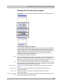
Switching to the "Movie
recording" mode
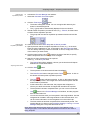
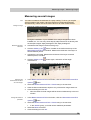
12. Select the Movie recording check box (1). The check box can be found below
the Live button in the Camera Control tool window.

Starting movie
recording
Stopping movie
recording
The Snap button will be replaced by the Movie button.
13. Click the Movie button to start the movie recording.

The live-image will be shown and the recording of the movie will start
immediately.

In the status bar a progress indicator is displayed. At the left of the slash
the number of already acquired images will be indicated. At the right of
the slash an estimation of the maximum possible number of images will
be shown. This number depends on your camera's image size and
cannot exceed 2GB.

on the Movie button indicates that a movie is being
This icon
recorded at the moment.
14. Click the Movie button again to end the movie recording.

The first image of the movie will be displayed.

The navigation bar for time stacks will be shown in the document group.
Use this navigation bar to play the movie.

The software will remain in the "Movie recording" mode until you clear
the Movie recording check box once more.
Acquiring a time stack
In a time stack all frames have been acquired at different points of time. With a
time stack you can document the way the position on the sample changes with
time. To begin with, for the acquisition of a time stack make the same settings in
the Camera Control tool window as you do for the acquisition of a snapshot.
Additionally, in the Process Manager tool window, you have to define the time
sequence in which the images are to be acquired.
Task
You want to acquire a time stack over a period of 10 seconds. One image is to
be acquired every second.
1. Switch to the "Acquisition" layout. To do this, use, e.g., the View > Layout >
Acquisition command.
Selecting an objective
Setting the image
quality
2. On the Microscope Control toolbar, click the button with the objective that
you want to use for the image acquisition.
3. Switch to the live mode, and select the optimal settings for your acquisition,
in the Camera Control tool window. Pay special attention to setting the
correct exposure time. This exposure time will be used for all of the frames in
the time stack.
4. Choose the resolution you want for the time stack's frames, from the
Resolution > Snap/Process list.
5. Find the segment of the sample that interests you and focus on it.
26
Acquiring images – Acquiring movies and time stacks
Selecting the
acquisition process
6. Activate the Process Manager tool window.
7. Select the Automatic Processes option.
8. Click the Time Lapse
button.

The button will appear clicked. You can recognize this status by the
button's colored background.

The [ t ] group will be automatically displayed in the tool window.
9. Should another acquisition process be active, e.g., Z-Stack, click the button
to switch off the acquisition process.

Selecting the
acquisition parameters
The group with the various acquisition processes should now look like
this:
10. Clear the check boxes Start delay and As fast as possible.
11. Specify the time that the complete acquisition is to take, e.g., 10 seconds.
Enter the value "00000:00:10" (for 10 seconds) in the Recording time field.
You can directly edit every number in the field. To do so, simply click in front
of the number you want to edit.
located to the right of the field, to specify
12. Click the button with the lock
that the acquisition time is no longer to be changed.
13. Specify how many frames are to be acquired.
Enter e.g., 10 in the Cycles field.

The Interval field will be updated. It shows you the time that will elapse
between two consecutive frames.
Acquiring a time stack
14. Click the Start
button.

The acquisition of the time stack will start immediately.

The Start Process button changes into the Pause
this button will interrupt the acquisition process.

button will become active. A click on this button will stop
The Stop
the acquisition process. The images of the time stack acquired until this
moment will be preserved.

At the bottom left, in the status bar, the progress bar will appear. It
informs you about the number of images that are still to be acquired.

The acquisition has been completed when you can once more see the
button. A click on
button in the Process Manager tool window, and the progress
Start
bar has been faded out.

You will see the time stack you've acquired in the image window. Use the
navigation bar located in the image window to view the time stack. You
can find more information on the navigation bar in the online help.

The time stack that has been acquired will be automatically saved. The
storage directory is shown in the Acquisition Settings > Saving > Process
Manager dialog box. The preset file format is VSI.
Note: When other programs are running on your PC, for instance a virus
scanning program, it can interfere with the performance when a time stack is
being acquired.
27
Acquiring images – Acquiring a Z-stack
00304
4.4. Acquiring a Z-stack
A Z-stack contains frames acquired at different focus positions. That is to say,
the microscope stage was located in a different Z-position for the acquisition of
each frame.
Note: You can only use the Z-Stack acquisition process when your stage is
equipped with a motorized Z-drive.
Acquiring a Z-stack
Example: You want to acquire a Z-stack. The sample is approximately 50 µm
thick. The Z-distance between two frames is to be 2 µm.
1. Switch to the "Acquisition" layout. To do this, use, e.g., the View > Layout >
Acquisition command.
Selecting an objective
Setting the image
quality
2. On the Microscope Control toolbar, click the button with the objective that
you want to use for the image acquisition.
3. Switch to the live mode, and select the optimal settings for your acquisition,
in the Camera Control tool window. Pay special attention to setting the
correct exposure time. This exposure time will be used for all of the frames in
the Z-stack.
4. Search out the required position in the sample.
Selecting the
acquisition process
5. Activate the Process Manager tool window.
6. Select the Automatic Processes option.
7. Click the Z-Stack
Selecting the
acquisition parameters
button.

The button will appear clicked. You can recognize this status by the
button's colored background.

The [ Z ] group will be automatically displayed in the tool window.
8. Select the Range entry in the Define list.
9. Enter the Z-range you want in the Range field. In this example, enter a little
more than the sample's thickness (= 50 µm), e.g., the value 60.
10. In the Step Size field, enter the required Z-distance, e.g., the value 2, for a Zdistance of 2 µm. The value should roughly correspond to your objective's
depth of focus.

In the Z-Slices field you will then be shown how many frames are to be
acquired. In this example 31 frames will be acquired.
9. Find the segment of the sample that interests you and focus on it. To do this,
use the arrow buttons in the [ Z ] group. The buttons with a double arrow
move the stage in larger steps.
Acquiring an image
10. Click the Start

button.
Your software now moves the Z-drive of the microscope stage to the
start position. The starting positions lies half of the Z-range deeper than
the stage's current Z-position.
28
Acquiring images – Acquiring an EFI image

The acquisition of the Z-stack will begin as soon as the starting position
has been reached. The microscope stage moves upwards step by step
and acquires an image at each new Z-position.

The acquisition has been completed when you can once more see the
button in the Process Manager tool window, and the progress
Start
bar has been faded out.

You can see the acquired Z-stack in the image window. Use the
navigation bar located in the image window to view the Z-stack. You can
find more information on the navigation bar in the online help.

The Z-stack that has been acquired will be automatically saved. You can
set the storage directory in the Acquisition Settings > Saving > Process
Manager dialog box. The preset file format is VSI.
Note: When other programs are running in the background on your PC, for
instance a virus scanning program, it can interfere with the performance when a
Z-stack is being acquired.
00367
4.5. Acquiring an EFI image
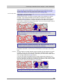
What is EFI?
EFI is the abbreviation for Extended Focal Imaging. By using the "EFI"
acquisition process you can acquire images with your microscope which have
practically unlimited depth of focus. To do this, EFI uses a series of differently
focused separate images (Focus series) to calculate a resulting image (EFI
image), that is focused in all of its parts.
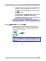
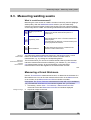
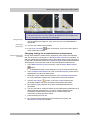
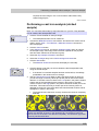
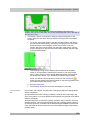
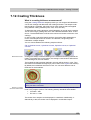
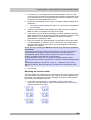
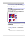
At the left hand-side, the illustration shows a number of frames that were
acquired at different Z-positions. In each of these frames there are only a few
image segments that are displayed sharply focused. These segments are shown
in color. These sharply focused image segments will be assembled into the EFI
image (right).
Creating an EFI image
Your software offers you several ways of creating an EFI-image.


Acquiring an EFI image without a motorized Z-drive
Acquiring an EFI image with a motorized Z-drive
29
Acquiring images – Acquiring an EFI image
Acquiring an EFI image without a motorized Zdrive
Task
You have a thick section in the transmitted light mode, or a sample with a very
rough surface in the reflected light mode, e.g., with holes, grooves, bumps peaks
or slanting planes. In the image it's only possible to bring one layer of the section,
or only part of the surface, sharply into focus, higher-lying or deeper-lying areas
are outside the depth of focus range. Acquire a Z-stack through the complete
thickness or height of the sample, and have the EFI image calculated for you.
In this case, you can use the manual Instant EFI acquisition process to acquire a
sharply focused image of all of the sample.
Note: You can use the Instant EFI acquisition process with every microscope.
When your microscope stage is equipped with a motorized Z-drive, use the ZStack acquisition process to acquire an EFI image.
Selecting the
acquisition process
1. Use the View > Tool Windows > Process Manager command to make the
Process Manager tool window appear.
2. Select the Manual Processes option.
3. Click the Instant EFI
Setting acquisition
parameters
button.

The button will appear clicked. You can recognize this status by the
button's colored background.

The Instant EFI group will be automatically displayed in the tool window.
4. From the Algorithm list, select the Reflected light entry, when you use your
light, or stereo microscope in the reflected light mode.
5. If you work with a stereo microscope, select the Automatic frame alignment
check box.
If you don't work with a stereo microscope, clear the Automatic frame
alignment check box.
Preparing an EFI
acquisition
6. Use the View > Tool Windows > Camera Control command to make the
Camera Control tool window appear.
7. In the Camera Control tool window, click the Live
button.
8. Move the microscope focus to the Z-position where either the lowest or the
highest place on the sample is only just no longer sharply focused. Use the
live-mode for a visual control.
9. Check the exposure time, and correct it if necessary. When the Instant EFI
acquisition process has been started, the exposure time will be kept constant
during the whole of the acquisition.
Acquiring an EFI image
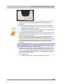
10. In the Process Manager tool window, click the Start
button.
30
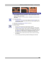
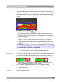
Acquiring images – Acquiring an EFI image

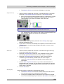
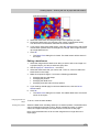
The live-image in the document group will divide itself into 3 images. On
the bottom right, you'll still see the live-image (3). On the bottom left,
you'll see the sharpness map (2). The large image above them is the
composite resulting image (1). The 3 images will be continually updated.
11. Use your microscope's Z-drive to move your stage slowly through the height
range of the sample's surface.

Your software will acquire images at the various focal planes, then it will
set them together. While this is being done, the camera will acquire the
images as quickly as possible. The sharpness value of individual pixels
will be calculated for every image. If the sharpness values are higher
than in the previous images, the pixels in the composite EFI image will
be adopted. The EFI image contains the pixels with the highest
sharpness values from all of the images acquired up till then.

The sharpness map at the bottom left will show you which image areas
will be sharply reproduced in the EFI image. The brighter a pixel is in the
sharpness map, the higher is its sharpness value in the EFI image.

Once the acquisition process has been started, the sharpness map
should only be bright at the deepest, or highest parts of the sample, the
rest of the map is dark.
12. Focus on the sample slowly once through all the focal planes.
After each change of the focus position, wait until you see that further areas
become brighter in the sharpness map.

As the process continues, more and more areas in the sharpness map
should become brighter. At the same time the EFI image will also get
better and better.
13. Check the EFI image and the sharpness map. Are all areas of the image now
sharp? Are there any areas in the sharpness map that are still dark?
Focus on these areas and have additional images calculated into the EFI
image. Continue acquiring additional images until the whole sample has
been sharply reproduced.
14. In the Process Manager tool window, click the Stop
button.

The resulting image is not a Z-stack, but a standard image.

The EFI image will be automatically saved. You can set the storage
directory in the Acquisition Settings > Saving > Process Manager dialog
box. The preset file format is VSI.
31
Acquiring images – Acquiring an EFI image
15. In the Camera Control tool window, click the Live
button again.
Acquiring an EFI image with a motorized Z-drive
Task
You have a thick section in the transmitted light mode, or a sample with a very
rough surface in the reflected light mode, e.g., with holes, grooves, bumps peaks
or slanting planes. In the image it's only possible to bring one layer of the section,
or only part of the surface, sharply into focus, higher-lying or deeper-lying areas
are outside the depth of focus range. Acquire a Z-stack through the complete
thickness or height of the sample, and have the EFI image calculated for you.
You can use the automatic Z-stack acquisition process to acquire a sharply
focused image of all of the sample.
Prerequisite: You can only use the Z-Stack acquisition process when your stage
is equipped with a motorized Z-drive.
Setting the EFI
parameters
1. Activate the Process Manager tool window.
2. To open the Acquisition Settings dialog box, click the Acquisition Settings
button in the tool window's toolbar.
3. Select the Acquisition > Automatic EFI entry in the tree view.
4. In the Algorithm list, select the Transmitted light (exp) entry, if you're working
in the transmitted light mode, and the Reflected light entry, if you're working
in the reflected light mode.
5. Select the Automatic frame alignment check box when you're working with a
stereo microscope and acquiring the sample at a viewing angle.
Otherwise, clear this check box.
6. Close the Acquisition Settings dialog box with OK.
Preparing for the
acquisition of a Z-stack
7. Carry out all the microscope settings.
8. On the Microscope Control toolbar, click the button corresponding to the
objective you've set.
9. Activate the Camera Control tool window.
10. Switch to the live mode.
11. Optimize the exposure time. The exposure time will be kept constant during
the acquisition of the Z-stack.
12. Click the Autofocus
to focus.
Setting the Z-stack
parameters
button in the Camera Control tool window's toolbar
13. Activate the Process Manager tool window.
14. Select the Z-Stack acquisition process.
15. Select the Top and bottom entry in the Define list.
16. Use the arrow buttons in the [ Z ] group to move your stage to the Z-position
at which the lowest-lying position on the sample is sharply focused.
The arrow buttons move the stage either by steps of 2 µm or of 20 µm.

The stage's current position will be shown to you in thePos. field.
17. Click the top Set button to define the starting position for the Z-stack
acquisition.

The current Z-position will be adopted in the End field.
18. Use the arrow buttons in the [ Z ] group to move your stage to the Z-position
at which the highest-lying position on the sample is sharply focused.
19. Click the bottom Set button to define the position at which the Z-stack
acquisition is to end.
32
Acquiring images – Acquiring an EFI image

The current Z-position will be adopted in the End field.
20. In the Step Size field, enter the distance between two frames in the Z-stack.
This Z-distance should be small enough to ensure that no positions on the
sample between two images remain blurred. The higher your objective's
Numerical Aperture is, the smaller the Z-spacing should be.
21. Use the [Enter] key to confirm the Z-distance that you've set.

Starting an EFI
acquisition
The number of images in the stack will be automatically calculated on the
basis of the Start and End values, and the Z-distance.
22. Select the Extended Focal Imaging (1) check box. You can find the check
box at the bottom of the [ Z ] group located in the Process Manager tool
window.
23. Finish the live mode.
24. Click the Start
button.

The EFI acquisition begins immediately.

The acquisition will begin. After the acquisition has been completed the
EFI image will be shown in the document group. This image was
calculated from the variously focused separate images.
00372 05072012
33
Acquiring images – Creating stitched images
4.6. Creating stitched images
What is a stitched
image?
If you acquire a stitched image, move the stage in a way that different, adjoining
parts of the sample are shown. All of the images that are acquired are combined,
just like a puzzle, into a stitched image. The stitched image will display a large
part of the sample in a higher X/Y-resolution than would be possible with a
simple snapshot.
The illustration shows left, four separate images. On the right you see the
stitched image made up from the four images.
Creating a stitched
image
Your software offers you several ways of creating a stitched image.





Materials science
analysis processes on
stitched images
Acquiring a stitched image without a motorized XY-stage (Manual MIA)
Acquiring a stitched image with a motorized XY-stage (XY-Positions /
MIA)
Acquiring a stitched image with extended depth of focus
Automatically acquiring several stitched images
Combining individual images into a stitched image
The Materials Solutions tool window offers several materials science analysis
processes. Most of these processes can also use stitched images an input,
provided that you are working with a motorized XY-microscope stage. The
acquisition of these stitched images are defined in the Stage path settings step
within the materials science analysis process. In this case, you won't need the
acquisition processes described in this topic.
Acquiring a stitched image without a
motorized XY-stage (Manual MIA)
Task
Prerequisite
You want to acquire an image of a large sample area. Use the Manual MIA
acquisition process to acquire several individual images of adjoining positions on
the sample, and to have them combined into a stitched image. MIA stands for
Multiple Image Alignment.
The camera is aligned parallel to the XY-stage. The angle between camera and
stage should be smaller than 1°.
1. Switch to the "Acquisition" layout. To do this, use, e.g., the View > Layout >
Acquisition command.
Selecting an objective
Setting the image
quality
2. On the Microscope Control toolbar, click the button with the objective that
you want to use for the acquisition of the stitched image.
3. Switch to the live mode, and select the optimal settings for your acquisition,
in the Camera Control tool window. Pay special attention to setting the
correct exposure time. This exposure time will be used for all of the stitched
image's individual images.
34
Acquiring images – Creating stitched images
4. Find the position on the sample at which you want to start acquiring the
stitched image.
5. Finish the live mode.
Selecting the
acquisition process
6. Activate the Process Manager tool window.
7. Select the Manual Processes option.
8. Click the Manual MIA button.

The button will appear clicked. You can recognize this status by the
button's colored background.

The Manual MIA group will be automatically displayed in the tool window.

Selecting the
acquisition parameters
Should the Instant EFI acquisition process have been active, it will be
automatically switched off. You can, however, use images with extended
depth of focus for the stitched image. To do this, before you acquire each
of the individual images, click the Instant EFI button located in the
Manual MIA group.
9. Make quite certain that the Auto Align button appears clicked. It should then
look like this:
.

Acquiring a stitched
image
Then your software will search for the same image structures in
neighboring individual images. The stitched image will be put together in
such a way that image areas that are the same will be superimposed.
10. Click the Start

button.
Your software switches into the live mode.
11. Bring the sample into focus.
12. Click on one of the arrow buttons to set the side of the current image at
which the next image is to be arranged. For example, click this button
the next image is to be laid to the right of the current image.

if
Your system now acquires an image at the current position on the
sample. In the image window you now see on the left (1) the acquired
image, and on the right (2) the live-image is displayed.
Since you haven't moved the sample, the live-image still shows the
current sample position, too, which means that you now see the current
image twice.
The two images overlap. Since the live-image is shown transparent, you
see both images in the overlap area simultaneously.
13. Make a note of a significant structure on the live-image's right border. You
will find the same sample structure in the overlap area. On the illustration, a
significant structure has been indicated by a circle.
35
Acquiring images – Creating stitched images
14. Now move the stage very slowly to make the structure on the live-image
move to the left. Keep moving the stage until the image structures in the
overlap area lie as exactly over each other as possible. The image structures
need not lie precisely over each other, since your software will match the
individual images with each other.

In the overlap area (3), the same image segments are shown now. This
enables your software to seamlessly combine the two images.

You can reverse the direction in which your stage moves, in the Device
Settings > Stage dialog box. Depending on how you can best orient
yourself, the live-image will then move to the left or to the right, when you
move your stage to the right.
15. Check whether both images have been correctly combined. Otherwise, you
can undo the last step by using the Undo last frame
button. You can then
move the stage again, and match the structures better.

During the acquisition, you can change the current stitched image's
zoom factor, e.g., to see certain parts in the overlap area better. You will
find an overview on the possibilities of changing an image's zoom factor
in the online help.
16. Define your way through the sample, with the arrow buttons, and follow that
with the stage.
In this manner, you can display a sample in any form you like in the stitched
image. The illustration shows a stitched image that is made up of 9 individual
images, and the stage path.
17. Click the Stop
stitched image.

button when you want to end the acquisition of the
You see the completed stitched image (4) in the image window.
Since the individual images can lie a little askew of each other, the
stitched image isn't as a rule, rectangular, but contains empty areas on
its borders (5). These areas will, as a rule, be cut off in the stitched
36
Acquiring images – Creating stitched images
image.
Properties of the
stitched image

The stitched image will, by default, be automatically saved. The storage
directory is shown in the Acquisition Settings > Saving > Process
Manager dialog box. The preset file format is VSI.

By default, in the overlap area, the intensity values of two adjoining
individual images will be matched with each other to make the image's
overall impression homogeneous.

Stitched images are calibrated. This means that you can measure
distances and objects on a stitched image.
37
Acquiring images – Creating stitched images
Acquiring a stitched image with a motorized
XY-stage (XY-Positions / MIA)
Task
You want to acquire an image of a large sample area. Use the automatic XYPositions / MIA acquisition process to scan a rectangular area of the sample and
to have adjoining images combined into one stitched image. MIA stands for
Multiple Image Alignment.
You can only use the XY-Positions/ MIA acquisition process if your microscope is
equipped with a motorized XY-stage.
Preconditions



The stage has been set up and initialized, i.e. its stage limits have been
defined.
The camera is aligned parallel to the XY-stage. The angle between
camera and stage should be smaller than 1°.
The shading correction has been set up.
1. Switch to the "Acquisition" layout. To do this, use, e.g., the View > Layout >
Acquisition command.
Selecting an objective
Selecting the
acquisition process
2. On the Microscope Control toolbar, click the button with the objective that
you want to use for the acquisition of the stitched image.
3. Activate the Process Manager tool window.
4. Select the Automatic Processes option.
5. Click the XY-Positions / MIA button.
Using the software
autofocus

The button will appear clicked. You can recognize this status by the
button's colored background.

The XY group will be automatically displayed in the tool window.
6. If your microscope is equipped with a motorized Z-drive, you can switch on a
software autofocus.
In the Process Manager tool window, click the Autofocus button.

The Autofocus group will be automatically displayed in the tool window.
7. In the Autofocus group, select the Multiposition / MIA check box.
8. If the sample surface is not plane or if it is inclined to the objective, choose
the Every MIA frame option. Now, the software autofocus will be performed
before every image acquisition.
Putting the stage
navigator on display
9. In the Process Manager tool window, click this button

.
The Stage Navigator tool window is shown. When you have acquired an
overview image of your sample, you will see this area of the image in the
stage navigator's image segment.
10. Set the magnification for the image segment in the Stage Navigator tool
window. To do this, use the zoom buttons at the bottom left of the tool
window (2).
The current stage position will be shown by a yellow rectangle in the image
segment (1). You should choose a magnification that enables you to see this
38
Acquiring images – Creating stitched images
rectangle clearly.

Defining the MIA scan
area
You can find more information on the Stage Navigator tool window in the
online help.
11. In the Process Manager tool window, click this button
.

The system will automatically switch into the live mode.

The Define MIA Scanning Area dialog box opens.
12. Move the XY-stage to the top left-hand corner of the MIA scan area you want
(3).
13. Focus, then select the optimal settings for your acquisition, in the Camera
Control tool window. Pay special attention to setting the correct exposure
time. This exposure time will be used for all of the stitched image's individual
images.
14. Confirm the starting position in the Define MIA Scanning Area dialog box with
OK.
15. Move the XY-stage to the bottom right-hand corner of the MIA scan area (4).
Confirm this position in the Define MIA Scanning Area dialog box with OK.

Acquiring a stitched
image
In the Stage Navigator tool window, the MIA scan areas that have been
defined are displayed. Here, you can immediately see how many
individual images are required for the acquisition of the stitched image,
when the current magnification is used.
16. Click the Start
button.
39
Acquiring images – Creating stitched images

The acquisition begins immediately. The individual images are acquired,
then immediately assembled. You can watch how the stitched image
grows, in the image window.

In the status bar at the bottom left of the user interface, you will find a
progress bar, the number of images already acquired, and the total
number of frames (e.g., 3/9).

The acquisition has been completed when you can once more see the
button in the Process Manager tool window, and the progress
Start
bar has been faded out.

You see the completed stitched image, in the image window. The
individual images won't be saved separately.

The stitched image will, by default, be automatically saved. The storage
directory is shown in the Acquisition Settings > Saving > Process
Manager dialog box. The preset file format is VSI.
40
Acquiring images – Creating stitched images
Acquiring a stitched image with extended
depth of focus
The acquisition of a stitched image with extended depth of focus, is both with and
without, a motorized XY-stage, possible.
Without a motorized
XY-stage
1. Start the Manual MIA acquisition process.
You can find a step-by-step instruction for doing this further above.
2. Click the Instant EFI

button, in the Manual MIA group.
The Instant EFI acquisition process will start at once. Instead of the liveimage, you now see the EFI image.
3. Now move your microscope's Z-drive slowly and change the focusing of the
image. Observe how the EFI image builds itself up.

For each image that is acquired, the sharpest image segment is adopted
in the EFI image.
4. When all of the image structures are sharply displayed, click one of the
direction arrows in the Manual MIA group to continue with the acquisition of
the stitched image.
Note: You now see the live-image with the last focus settings. That means that
normally, the live-image won't be in focus.
5. Bring the image into focus.
6. Repeat the last steps for each of the stitched image's individual images for
which you want to use the Instant EFI acquisition process.
7. Click the Stop
stitched image.

With a motorized XYstage
button when you want to end the acquisition of the
You see the completed stitched image, in the image window.
You can only use the EFI acquisition process when your stage is equipped with a
motorized Z-drive.
1. Select the XY-Positions / MIA acquisition process.
2. Define an MIA scan area.
You can find a step-by-step instruction for doing this further above.
3. Additionally, select the Z-Stack acquisition process.

In the group with the different acquisition processes, two of them are now
active:
4. Define all of the parameters for the Z-stack's acquisition.
5. In the [ Z ] group, select the Extended Focal Imaging check box.
6. Click the Start

button to begin the acquisition of the stitched image.
At each of the MIA scan area's stage positions, a Z-stack will first be
acquired, then the EFI image calculated from it. The EFI images will be
combined into a stitched image.
41
Acquiring images – Creating stitched images

When the acquisition process has been completed, you'll see the
finished stitched image in the image window.
Automatically acquiring several stitched
images
You can define several MIA scan areas on the sample. When the acquisition has
started, all of the MIA scan areas will be moved to, one after the other, and a
stitched image will be acquired at every position.
1. Select the XY-Positions / MIA acquisition process.
2. Define several MIA scan areas. You can find a step-by-step instruction on
how to define an MIA scan area further above.
Begin with the area of the sample that is to be scanned first.
Putting the stage
navigator on display
Acquiring stitched
images
3. In the Process Manager tool window, click this button
.

The Stage Navigator tool window is shown. When you have acquired an
overview image of your sample, you will see this area of the image in the
stage navigator's image segment.

In the Stage Navigator tool window, the MIA scan areas that have been
defined are displayed. They are numbered serially in the order in which
they were defined.
4. Click the Start
button to begin the acquisition of the stitched image.

Each of the MIA scan areas will now be scanned, and the stitched image
created. The scan areas will be scanned in the order that is predefined
by the numbering.

All of the stitched images will be acquired with the current camera, and
current acquisition settings.

When the acquisition process has been completed, you'll find a stitched
image for each of the MIA scan areas, in the document group.
42
Acquiring images – Creating stitched images
Combining individual images into a stitched
image
Use the Process > Multiple Image Alignment… menu command to have several
separate images combined, as with a puzzle, into a stitched image. The
individual images will be combined in their full X/Y-resolution. The stitched image
will thus display a large sample segment in a higher X/Y-resolution than would be
possible with a single acquisition.
Acquiring images
Selecting images
1. Load the images you want to combine, or acquire a suitable set of images.

All of the images you want to combine must be of the same image type.
You can't, e.g., have a gray-value image combined with a true-color
image.

When you acquire the images, number their names sequentially, e.g.,
"Image001", "Image002" and so on. In many cases, the images will then
already be arranged in the right order in the Multiple Image Alignment
dialog box.
2. Open the Gallery tool window. To do this, use, e.g., the View > Tool
Windows > Gallery command.
3. Select all of the images you want to combine in the Gallery tool window.
Assembling images
4. Use the Process > Multiple Image Alignment... command. This command is
only active when more than one image of the same image type has been
selected.

The Multiple Image Alignment dialog box opens.

The dialog box's stitching area will display a preview of the individual
images.
5. If necessary, while keeping your left mouse button depressed, drag on the
bottom left-hand corner of the dialog window to enlarge it. Alternatively,
double click the header of the dialog box to enlarge the dialog box to fullscreen size.
6. Check whether the images' positions are correct. You can change the
arrangement of the individual images, e.g., by exchanging two images in the
stitching area by
Drag&Drop.

The illustration shows the stitching area with four individual images. On
the left, the images 1 and 2 are not in the correct position. Image 1
(green frame) will therefore be dragged onto image 2 (red frame). On the
right, you see the stitching area after the two images have been
interchanged.
7. When the individual images overlap, select the Correlation option in the
Output > Alignment list.
Then your software will search for the same image structures in neighboring
43
Acquiring images – Creating stitched images
individual images. The stitched image will be put together in such a way that
image areas that are the same will be superimposed.
8. Click the OK button to carry out the automatic image alignment.
Checking a stitched
image

The Multiple Image Alignment - Manual Align dialog box opens.

The stitched image will be displayed.
9. Check the stitched image on display.
Use the zoom buttons in the dialog box to zoom in the stitched image in the
dialog box.
10. Should individual images have been incorrectly assembled, you can
manually shift one or more of them, in respect to one another.
To do this, click in the image you want to shift, then drag it with your left
mouse button depressed, in the required direction.

The currently selected image will be displayed semi-transparently to
make it easier for you to find the point of contact with the neighboring
image.

Two images were not correctly aligned with each other. There is a
misalignment. When the manual alignment has been made, the two
images fit together seamlessly.
11. Select the Cut Edges check box to clip the image in such a way that there
are no longer any empty areas visible on its borders.

In the preview, the image edges that are to be clipped will be displayed
semi-transparently.
12. Select the Equalize check box if the images aren't homogeneously
illuminated. Then the intensity values of the individual images will be
matched with one another, which will make the background appear more
homogeneous.
13. Click OK.

A new image with the name "Image_<consecutive No.>" will be created.
00383
44
Processing images – Commenting images
5.
Processing images
5.1. Commenting images
There are several different ways of adding notes to an image.
Using drawing objects
The Drawing toolbar makes a variety of drawing functions (line, rectangle, ellipse,
text) available to you, as well as options for color selection and line styles.
You can find more information on working with drawing objects in the online help.
Using annotations
You can use the Annotations tool window to mark interesting positions in an
image, to name them and to save them. You can give each position a text or
audio annotation. In this way you will be able to jump to the position in the image
that you want with one mouse click, and this will be immediately shown in the
magnification you want.
Use this possibility especially when you are commenting on very large images.
You can find more information on working with positions and views in the online
help.
Entering an image
comment
The Properties tool window will show you all of the available information from the
document group on the active image.
You can also supplement this information with a text annotation of your own on
the image. Enter your comment in the Note field. You can find step-by-step
instructions in the online help.
00121
5.2. Processing images
The Process menu offers numerous image processing functions, with which you
can change an acquired image (e.g., increase the image contrast or the image
sharpness).
1. Load the image you want to process, or activate the image in the document
group.

Please note that the Process menu will only be visible when an image
window is active in the document group.
2. Use one of the commands in the Process menu, e.g., Process >
Enhancement > Adjust Intensity... .

The image processing dialog box will open. The image processing
operation that is active will be shown in the dialog boxes header.
3. Click the small arrow next to the Preview
button to open a list of all of
the preview functions. Select the Original and Preview entry.

This preview function displays the same image segment twice in the
dialog box. The first one shown is the source image. The second is the
image that results when the current parameters are used.

Most of the image processing operations need one or two of the
parameters that are shown in the Settings group.
4. Change the image processing operation's parameters. After every change
that is made in a parameter, the operation will be immediately applied to the
source image, and the resulting image will be shown in the preview window.
Click the Default button to readopt the preset parameters in the Settings
group, when the current parameter doesn't make sense to you.
45
Processing images – Processing images
5. When you have found the optimal parameters, click the OK button to have
the active image processing operation applied to the image with the active
parameters.

The image processing dialog box will closed.

Please note that the image processing operation changes the source
image. No new image document will be created. You can, however use
the Edit > Undo command to restore the source image.
00175
46
Measuring images – Overview
6.
Measuring images
6.1. Overview
Your software offers a wide range of measurement functions. They enable you to
quickly count objects and measure segments and areas. All the results will be
saved together with the image and can also be issued as a sheet.
Prerequisite: For making measurements, correctly calibrated images are an
essential prerequisite. Images that you have acquired with your software will
have been automatically correctly calibrated when you have specified the
objective you used.
Should the image not yet have been calibrated, use the Image > Calibrate
Image... command to carry out a calibration.
Selecting the measurement environment
Measuring with help of
the tool window
Switch to the Processing layout when you want to measure images. You can find
the Measurement and ROI tool window in the bottom section of this layout. In this
tool window you have fast access to all measurement functions and settings
which relate to the measurement. This tool window is at the same time the
measurement display and contains all of the values that have been measured on
the active image.
Note: Should, right at the bottom of the user interface, several tool windows lie
one over the other, activate the Measurement and ROI tool window, by clicking
on the header of the
Measurement and ROI tab. The tabs can be found
under the tool windows.
Starting a measurement
Begin a measurement by selecting the measurement function you want. You will
find the measurement function in the Measurement and ROI tool window, on the
Measurement and ROI toolbar, or in the Measure menu.
Working in the
measurement mode
As soon as you have clicked a measurement function, your software will
automatically switch to a measurement mode. In the measurement mode your
mouse pointer will take on the shape of a cross on the image. You can make as
many measurements as you like with the measurement function that has been
selected. The continuous measurement mode is valid for all loaded images. You
can, therefore, easily measure numerous images one after the other.
The selected measurement function's button will keep its clicked appearance and
in this way show you the current measurement function. You can recognize this
status by the button's background color.
Finishing the
measurement mode
You will remain in this measurement mode until you explicitly switch it off. To do
so, click the Select Measurement Objects
button. You can find the button
either in the Measurement and ROI tool window or on the toolbar.
Changing the default
measurement mode
The continuous measurement mode described above is preset by default. You
can change this default setting. To do this, use the Tools > Options... command.
Select the Measurement and ROI > General entry in the tree view. Select the
Switch to 'Select Measurement Objects' mode after creating a measurement
object check box. Then, when you have completed a measurement, you will
automatically leave the measurement mode again. This means you have to
select the measurement function again before you start each interactive
measurement.
47
Measuring images – Overview
Displaying and saving measurement results
The measurement results will be displayed directly on the image and in the
Measurement and ROI tool window. Use the View > Tool Windows >
Measurement and ROI command to have the tool window displayed.
Saving the
measurement results
The measurements will be saved along with the image, if you save the image in
the TIF or VSI file format.
You can, however, also export the measurement results in a results sheet, and
save this as a file. To do this, use the Export to Excel or Export to Workbook
command. You find both of the commands, e.g., in the Measure menu.
Showing and hiding
measurement results in
an image
The measurement results will be shown on the image in a special data layer, the
measurement layer. On your monitor, image and measurement layer are shown
together. The data of each, however, is individually stored if you use the TIF or
VSI image file format. Try and picture the measurement layer as a transparency
which is placed over the image. When you measure an image, the image data
will not be changed by having the measurement results displayed on it.
You can, at any time, hide or show the measurement layers.
To do so, use the Layers tool window. There you have access to all of an image's
layers. The eye icon
identifies all of the layers that are currently on display on
your monitor.
Click the eye icon in front of the measurement layer to hide the measurements.
Click an empty cell without an eye icon to make the corresponding layer
reappear.
Editing measurements
You can edit existing measurement objects at any time. To do so, click the Select
Measurement Objects
button. You can find the button either in the
Measurement and ROI tool window or on the toolbar.
Note: When you load an image file with measurement objects, it is only possible
to edit the measurement objects if the image file has been saved in the TIF or
VSI image file format.
Moving measurement
objects
You can move a measurement object while keeping the left mouse button
depressed.
Increasing/decreasing
the size of
measurement objects
You can also change the size of a measurement object. Move the pointer onto a
marker. By dragging the marker with the mouse button depressed, you can
adjust the frame's size as wished.
Deleting measurement
object
Click the [Del] key on your keyboard in order to delete the selected measurement
object.
What happens to the
measurement values?
The measurement values in the Measurement and ROI tool window will be
correspondingly updated.
Changing the color, font
and line thickness of
individual measurement
objects
You can, at any time, change the color, font, and line thickness, of individual
measurement objects. Select one or more measurement objects in an image and
click your right mouse button to open a context menu. In the context menu you'll
find several commands with which you can change the appearance of the
selected measurement objects.
From the context menu, select, e.g., the Change Color... command. Select the
color you would like from the color palette, then close the dialog box with OK.
48
Measuring images – Overview
Measuring in the live mode
All of the measurement functions are also available in the live-image. You can
therefore, e.g., quickly measure a segment in the live-image.
Measuring on different image types
Measuring on
multi-dimensional
images
You can combine a series of individual images into one image. What results is
e.g., a time stack in which all of the frames will have been acquired at different
times.
You can make measurements on every separate image. Display the required
frame on your monitor. To do this, use the navigation bar in the image window.
Then carry out the measurement on this frame. The measurement will be
permanently linked to this frame, i.e., the measurement will only be displayed on
your monitor when the frame on which you made this measurement is also on
display.
The measurement results will be shown in the Measurement and ROI tool
window. You can give every measurement the number of the frame on which it
was made. To do so, use, e.g., the measurement parameter Index t for time
stacks.
Measuring on
multi-layer images
With some functions, e.g., with the Image > Combine Color Images... function, a
multi-layer image will be created. This multi-layer image is made up of several
layers. You can find more information on multi-layer images in the online help.
Measurements always apply to one image layer. For this purpose, show the
image layer on your monitor, on which you want to make measurements. To do
so, use the Layers tool window. Then carry out the measurement on this image
layer. The measurement will be permanently linked to this image layer, i.e., the
measurement will only be displayed on your monitor when the image layer on
which you made this measurement is also on display.
The measurement results will be shown in the Measurement and ROI tool
window. You can give every measurement the name of the image layer on which
it was made. To do this, use the Layer measurement parameter.
Measurement precision
How precise the measurement is, depends on the X/Y-calibration and the
image's current zoom factor.
Influence of the X/Ycalibration
The X/Y-calibration defines the width and height of the sample area that is
represented by one pixel. For example, it could be that one pixel displays a
sample area of 10 µm x 10 µm. A pixel is the smallest image structure that can
be measured. For this reason, the maximum measurement precision where this
example is concerned, is 10 µm.
Influence of the zoom
factor
The zoom factor tells you how large the image will be displayed on your monitor.
With a zoom factor of 100%, one pixel on the monitor equals exactly one pixel in
the image. With a zoom factor of 50%, one pixel on the monitor equals 2 x 2
pixels in the image. When you make a measurement, you should use the zoom
factor 100% whenever possible. Then you will achieve a maximum of
measurement precision. Should the zoom factor 100% not be possible, because
the image area you want to measure can't then be completely seen, choose the
largest possible zoom factor under 100%.
Information about changing an image's zoom factor can be found in the online
help.
00150 02072012
49
Measuring images – Measuring images
6.2. Measuring images
Your software offers a wide range of measurement functions. They enable you to
quickly count objects and measure segments and areas.
The following step-by-step instructions present the measurement functions to you
by way of several examples.
Measuring image objects interactively
Task
You want to measure the filaments in a supraconductor.
To do this, load a suitable image, or acquire one. Measure the diameter of
several of the hexagonal filaments, in each case between the opposing vertices.
Subsequently edit the measurement. Delete some of the measurements you've
made. Enter the results in a MS-Excel sheet.
1. If necessary, use the View > Tool Windows > Measurement and ROI
command to have the Measurement and ROI tool window displayed.

Loading an image
You'll find the tool window at the lower edge of the user interface. It's
possible that it may be covered by the Count and Measure Results tool
window. Click the Measurement and ROI tab at the bottom of the user
interface to bring the tool window into the foreground.
2. Acquire an image or load one.
During the installation of your software some sample images have been
installed, too. You can follow these step-by-step instructions when you use
the example image "SupraConductor.tif".
Setting the labeling
color
The measurement results will be written into the image according to the default
settings, in red font color and without a background. This can't be easily read
against the superconductor's structure. Change the labeling settings.
1. Use the Tools > Options... command.
2. Click the Measurement and ROI > Measurement Display entry in the tree
view.
3. Click in the Background Color field, and choose, e.g., the color Black.
4. Select the Text color > Fixed colors option, then select the color White from
the palette, to see the measurements in white and the labeling in black, in the
image.
5. Close the dialog box with OK.
50
Measuring images – Measuring images
Measuring lengths
1. Click the Arbitrary Line
tool window.
button, located on the toolbar at the top of the
2. Click with your left mouse button at the starting point and end point of the
reference distance.
3. If you have measured a reference distance, you can immediately proceed
with the next measurement.
4. Click the Arbitrary Line
button again, to end the length measurement.
5. Take a look at the results in the tool window and in the image.

Deleting measurements
The illustration shows the image with three executed measurements.
The measurement 2 has been selected.
1. Click one of the measurement results in the Measurement and ROI tool
window.

The corresponding line will be marked in the image.
2. Press the [Del] key.

The measurement will be deleted both in the image and in the tool
window.

When a measurement has been deleted, the image and the tool window
contain one measurement less. The IDs of the remaining measurements
won't be changed by the deletion of a measurement.
When you've completed the measurements, you should switch off the
measurement mode, since otherwise, you might inadvertently select your
measurements and move them.
3. Check whether one of the buttons on the Measurement and ROI tool
window's toolbar appears clicked. Release this button
51
Measuring images – Measuring images
Exporting results to
MS-Excel
1. To do this, click the Export to Excel
button.
2. In the In/Output dialog box you set up the directory in which the data is to be
saved, and enter the name of the MS-Excel sheet. Adopt the file type "ExcelSheet (*.xls)“.
3. Click the Save button to have the MS-Excel sheet with the measurement
results saved.
Closing the image
1. Click the Close

button, located at the top right of the document group.
You have changed the image because you've added interactive
measurements. For this reason, you'll receive a query whether you wish
to save the image or not.
2. Save the image in the TIF or VSI file format. The measurements will then
also be saved in the image file. They can at any time, be edited deleted or
augmented.
Outputting various measurement parameters
Task
You want to measure the filaments in a supraconductor.
Measure the hexagonal structure as a circular surface. Have a variety of
measurement parameters, such as the area, the perimeter and the diameter,
output. Have the diameter shown in the image.
1. Acquire an image or load the "Supraconductor.tif" example image.
Measuring areas
2. In the Measurement and ROI tool window, click the 2 Points Circle
button.
3. With your left mouse button, click in the center point of the hexagonal
structure.
4. Move your mouse, and in the process drag out the circle. Match the circular
object as well as possible to the structure. Click the left mouse button.
5. Click the 2 Point Circle
mode.
button again, and switch off the measurement
6. Take a look at the result in the Measurement and ROI tool window.

Viewing the list of
measurement
parameters
The illustration shows the image of the superconductor with a circular
measurement.
1. In the Measurement and ROI tool window, click the Select Measurements
button.

In the dialog box you'll see a list with all of the available measurement
parameters. At the bottom of the dialog box you'll see a list of the
measurement parameters that are calculated for all objects.
52
Measuring images – Measuring images

Outputting additional
measurement
parameters
A detailed description of this dialog box can be found in the online help.
2. Go to the list of all of the available parameters, then click the "Diameter"
measurement parameter.

On the right, an illustration shows you how the parameter is calculated.
You can see that there are different ways in which the diameter of a 2D
object can be calculated.
3. Click the "Mean" entry in the list under the illustration to select the "Mean
(Diameter)" measurement parameter. When you do this, the mean value of
all of the possible diameters is determined.
4. Click the Add 'Mean (Diameter)' button.

This measurement parameter will be adopted in the list. All of these
measurement parameters will be displayed in the tool window.
5. Close the dialog box with OK.
6. Take a look at the result for the circle's diameter in the Measurement and
ROI tool window.
Outputting
measurement
parameters in the
image
1. Open the Select Measurements dialog box.
2. At the bottom of the list of all of the calculated measurement parameters,
click the "Mean (Diameter)" measurement parameter.
. Click this
3. To the right of this list you'll see a button with a blue arrow
button to move the measurement parameter to the top of the list.
4. Close the dialog box with OK.
5. Take a look at the result for the circle's diameter in the image.
Note: The measurement display in the image has to be updated once, so that the
settings that have been changed are also taken into account. You update the
measurement display, for instance, by adding another measurement, or by once
selecting an existing measurement in the image.
53
Measuring images – Measuring images
Measuring several images
Task
Loading an image
You want to measure the thickness of a spray coating. To do so, you acquire
several images of the coating. Have the results from all images displayed
simultaneously. Take a look at the mean value for all of the measurements.
1. Acquire an image or load one.
During the installation of your software some sample images have been
installed, too. You can carry these step-by-step instructions out directly with
the example images "SprayCoating2.tif" and "SprayCoating4.tif".
Measuring the layer
thickness
2. Activate the first image in the document group.
3. Click the Arbitrary Line
button, located on the toolbar at the top of the
Measurement and ROI tool window. Measure the thickness of the layer at
several different places.
4. Activate the next image. Measure the thickness of the layer at several
different places, here also.
5. Click the Arbitrary Line
measurement.

Displaying the
measurement results of
all of the images
button again, and switch off the length
The layer's thickness has been measured on both images.
1. In the Measurement and ROI tool window, click the Measurement and ROI
Options
button.
2. Select the Measurement and ROI > Results entry in the tree view.
3. Clear the Show measurement objects: Only of the active image check box.
4. Close the dialog box with OK.

Viewing the statistical
parameter
Now the results for both images will be shown simultaneously in the tool
window.
1. In the Measurement and ROI tool window, click the Measurement and ROI
Options
button.
2. Select the Measurement and ROI > Results entry in the tree view.

In the Statistic group, you'll find various statistical parameters.
3. Select the Mean check box.
4. Close the dialog box with OK.
54
Measuring images – Measuring images

Now, in the Measurement and ROI tool window under the measurement
results, the chosen statistical parameter (1) will by shown. You can see
there the mean value of the layer thickness for all of the measured
images.
Measuring heights
Task
To be able to make height measurements, you need to have a height map. A
height map is a gray-value image whose gray values contain height information.
The multi-dimensional image "Clockwork" is a Z-stack. Use the EFI algorithm to
calculate the height map. Measure the height difference between the brasscolored gear wheel in the middle image segment, and the silver-colored gear
wheel on the right-hand side of the image.
1. Load the "Clockwork.tif" image.

Creating a height map
The "Clockwork.tif" image is a Z-stack. The works of a clock was
analyzed under a reflected light microscope. In the process, images of
the works were acquired at different focus positions.
In the illustration, the Z-stack is displayed in the tile view. Pay attention to
the gear wheel that is only sharply reproduced in the middle of the Zstack.
2. Use the Process > Enhancement > EFI Processing… command.
3. Select the Apply on > All frames and channels option.
4. In the Algorithm list, select the Reflected light entry.
5. Select the Height map check box.
6. Select the Create new document as output check box.
7. Close the dialog box with OK.
55
Measuring images – Measuring images

You can see the EFI image with the clockwork's texture. The resulting
image is a multi-layer image and is therefore accompanied by this icon
in the image window's title.

The height map is a layer of the EFI image. The texture image makes up
the second layer. The height information is therefore also present in the
EFI image. You can measure the height directly on the texture image.
Measuring height
1. In the Measurement and ROI tool window, click the 3D Line
button.
2. Now measure the height between two image objects.
Click, for example, the brass-colored gear wheel, and the silver-colored gear
wheel on the right-hand side of the image.
3. Click the 3D Line
button in the Measurement and ROI tool window
again, then switch off the 3D measurement.

Issuing the height
difference
In the Measurement and ROI tool window, and in the image, the "3D
Length" measurement parameter is output with the line's complete
length.
The "3D Intensity Projection" measurement parameter measures the
height difference between two points.
1. In the Measurement and ROI tool window, click the Select Measurements
button.
2. In the list of all of the available measurement parameters, take a look at the
parameter of the "3D Line" object type.
3. Select the measurement parameter „3D Intensity Projection“.
4. Insert this measurement parameter into the list of the displayed
measurements.
5. Close the dialog box with OK.

In the tool window, you'll now see the "3D Intensity Projection"
measurement parameter. It tells you how far in height the two gear
wheels are from each other.
56
Measuring images – Measuring images
Viewing the height map
1. Use the View > Tool Windows > Layers command to make the Layers tool
window appear.
2. In the Layers tool window, click the [+] sign (1) and open the image's layers.

You can now see the image's individual layers. Height map (2) and
texture image (3 ). The height map can't be seen, because it's absolutely
transparent at the moment.

The measurements are on another layer (4).
3. Select the height map in the Layers tool window.
4. Click the Set Layer Opacity (5) button, located on the toolbar at the top of the
tool window.
5. Drag the slider all the way to the right, to an opacity of "100%", then take a
look at the height map.

Showing/hiding layers
Low-lying structures can be recognized by their dark gray values,
structures that lie higher, by their bright gray values.
to make the corresponding layer disappear. By doing
1. Click its eye icon
this, you can, e.g., for a time, remove the measurements from the image.
2. Click an empty cell without an eye icon to make the corresponding layer
reappear.
00154
57
Measuring images – Measuring welding seams
6.3. Measuring welding seams
What is a weld measurement?
Measuring the cross section of a weld is a method commonly used for judging a
weld's quality. With the Weld Measurement solution you can interactively
measure microscope images of weld cross-sections and can output the results
on the image and in a table. The following measurement functions are available:
Starting a
measurement
Interactive
measurement functions
and weld
measurements
Multiple perpendicular
lines
Use this measurement function, to determine the
distance from several measurement points to a
reference line.
Asymmetry Lines
Use this measurement function, to construct the
perpendicular bisector of the connection between two
reference points,
and to determine the distance of a measurement point
from the perpendicular bisector.
Throat thickness
Use this measurement function, to determine the
thickness of a fillet weld's throat.
You will find the weld measurement functions in the Measure menu, or as a
button on the Measurement and ROI tool window or toolbar. Start a
measurement, e.g., by clicking the corresponding button.
The functions which you can use to measure welds, behave just like the other
interactive measurement functions offered by your software, e.g. the Arbitrary
Line measurement function. All of the information on the interactive
measurement functions also applies for the measurement of welds.
10802
Measuring a throat thickness
Use the Throat thickness measurement function, to determine the thickness of a
fillet weld's throat. You can find the measurement function in the Measure menu,
or as a button on the Measurement and ROI tool window or toolbar.
Prerequisite: The Throat Thickness measurement function will only be available if
you purchased the Weld Measurement solution together with your software.
1. If necessary, use the View > Tool Windows > Measurement and ROI
command to have the Measurement and ROI tool window displayed.
Loading an image
2. Acquire an image or load one.
58
Measuring images – Measuring welding seams
The illustration shows a cross section of two welded pieces of metal. The weld is
circled.
How thick is the weld's throat?
3. Set a zoom factor for your image window that will make the image segment
that is to be measured clearly visible. You will achieve the most precise
measurements if you set the zoom factor at 100%.
Measuring the throat
thickness (with a
welded root)
4. Start the measurement. To do so, click the Throat Thickness
the toolbar at the top of the tool window.
button, on
With four mouse clicks (1-4), define two lines along the inner surfaces of the
metal pieces which are welded together.
5. Click on a point on the inner surface of the first piece of metal (1). This point
should be a far as possible from the weld's root. You can put the
measurement point before or after the weld.

The point which you define will be shown in the image with a handle.

The mouse pointer's shape on the image window shows which
measurement mode you are in.
6. With three more mouse clicks (2-4), define two lines along the inner surfaces
of the metal pieces which are welded together.

Your software will now automatically display some lines and handles in
the image window.

The mouse pointer is now linked to an auxiliary line, which is
perpendicular to the bisector of the angle. When you move the mouse
you will move this line at the same time.
Once the inner surfaces are defined (yellow lines), the position of the root (1) will
automatically be drawn in and your software will calculate the bisector of the
angle (2). Together with the handle (3), move the line (4) which is perpendicular
to the bisector of the angle to determine the throat thickness.
59
Measuring images – Measuring welding seams
7. Move the auxiliary line (4) to the outer surface of the weld. The part between
the two lines shown in yellow above must be just inside the cross-section of
the weld along the entire length.

The measurement of the throat thickness is thus complete. The Throat
Thickness measurement object (an equilateral triangle) is completely
defined.

The throat thickness (the height of the triangle) will be shown in the
image. In the Measurement and ROI tool window table, a new
measurement value with a type of Throat Thickness will be entered.
Note: If the measurement results are not shown, check the measurement
parameters currently displayed. You can find step-by-step instructions to modify
the measurement parameters further down.
8. Take a look at the result in the Measurement and ROI tool window and in the
image.
The illustration shows an enlargement of the weld with the measurement object
(an equilateral triangle). The result of the measurement is the throat thickness (1)
(the height of the triangle). The auxiliary line (2) (the base of the triangle) must be
positioned so that it just lies completely within the weld.
Measuring the throat
thickness (when the
root is exposed)
If the root of the weld is exposed, another step will be required to measure the
throat thickness.
9. Select the measurement object.
To do so, click the Select Measurement Objects
button to switch to a
selection mode and then click on the measurement object in the image
window. You can find this button, e.g., on the Measurement and ROI tool
window's toolbar.
Directly after a throat thickness measurement, the measurement object will
automatically be selected.
10. Click on the vertex.
11. Keep the left mouse button pressed and drag the vertex towards the outer
seam of the weld towards the base of the triangle). In this way you are
moving a second auxiliary line. This auxiliary line must also lie with its full
length just within the weld's cross section.
60
Measuring images – Measuring welding seams
If the root of the weld is exposed, drag another auxiliary line (3) from the vertex
(1). The throat thickness is now the distance (2) between the two auxiliary lines
which are perpendicular to the bisector of the angle.
Saving the image
Finishing the
measurement
12. Save the image in the TIF or VSI file format. The measurements will then
also be saved in the image file. They can at any time, be edited deleted or
augmented.
13. You can now measure other images.
button is still active, click on the button again to
14. If the Throat Thickness
finish measurement mode.
Changing settings for a throat thickness measurement
Adjusting measurement
parameters
During each interactive measurement, significantly more values are measured
than can be shown in the image or in the Measurement and ROI tool window. To
alter the measurement parameters shown, follow these step-by-step instructions.
In particular, ensure that at least the Length and Angle measurement parameters
are displayed, as they are both used for the throat thickness measurement.
1. In the Measurement and ROI tool window, click the Select Measurements
button.

A detailed description of this dialog box can be found in the online help.
2. In the Available measurements list, click on the Measurement column title to
alphabetically sort all of the parameters.
3. Select the Length measurement parameter in the Available measurements
list. This measurement parameter corresponds to the throat thickness.
button, to have the Length measurement
4. Click the Add 'Length'
parameter added to the list of calculated measurement parameters.
5. Also add the Angle parameter to the list of calculated measurement
parameters.
6. You can now further modify the display of the measurement parameters for a
throat thickness measurement. You can for instance delete all other
measurement parameters currently shown, so that the list of the
measurement results becomes clearer.
7. Close the dialog box with OK.
8. Do a throat thickness measurement and examine the result in the
Measurement and ROI tool window.
61
Measuring images – Measuring welding seams
Displaying measured
angles in addition to the
throat thickness in the
image
By default, for a throat thickness measurement, the measurement will be shown
in the image. You can also output the angle between the two pieces of metal
which have been welded together in the image.
1. Carry out a throat thickness measurement or load an image which contains a
throat thickness measurement.
2. Select the measurement object on the image. For example, select the
corresponding measurement in the Measurement and ROI tool window.
3. Click the right mouse button and select the Create Angle
the context menu.
command in

In addition to the throat thickness, the angle measured will also be
shown in the image.

This command creates another measurement object of type Angle. In the
Measurement and ROI tool window you will thus see two entries for the
measured weld.
Note: The measurements on a screen will automatically be numbered in
sequence. The angle measurement will thus always have a different
measurement ID from the associated throat thickness measurement. You can
switch off the display of the measurement IDs, if you find their display distracting.
To do so, open the Tools > Options > Measurement and ROI > Measurement
Display dialog box, and clear the Show ID check box.

With the commands in the context menu you can change the color of the
labels, of the measurement lines, the reference lines or you can even
alter the font.
4038
Performing an asymmetry measurement
Use the Asymmetry Lines measurement function to construct the perpendicular
bisector of the connection between two reference points and to determine the
distance of a measurement point from the perpendicular bisector. You can find
the measurement function in the Measure menu, or as a button on the
Measurement and ROI tool window or toolbar.
Prerequisite: The Asymmetry Lines measurement function will only be available if
you purchased the Weld Measurement solution together with your software.
1. If necessary, use the View > Tool Windows > Measurement and ROI
command to have the Measurement and ROI tool window displayed.
Loading an image
2. Acquire an image or load one.
3. Set a zoom factor for your image window that will make the image segment
that is to be measured clearly visible. You will achieve the most precise
measurements if you set the zoom factor at 100%.
Measuring asymmetry
4. Start the measurement. To do so, click the Asymmetry Lines
the toolbar at the top of the tool window.
button, on
62
Measuring images – Measuring welding seams
The illustration shows a cross section of two welded pieces of metal. How
asymmetric is this weld? Click on the two reference points (1) and (2) in turn.
Your software will automatically calculate the perpendicular bisector as a
reference line for the measurement of the asymmetry (3).
5. With the left mouse button, click on two reference points in turn.
The perpendicular bisector of the connecting line between these two
reference points is the reference line for the measurement of the asymmetry.
In the example shown, the reference points define the width of a weld. The
reference points in the example shown lie horizontally next to one another.
They could just as well have any orientation in the image.

The points which you define will each be marked in the image.

The mouse pointer's shape on the image window shows which
measurement mode you are in.

The mouse pointer is now linked to an auxiliary line, parallel to the
perpendicular bisector. When you move the mouse you will move this
line at the same time.
6. Left click a measurement point to measure its distance from the reference
line.

The result of the measurement will be shown in the image.
Define a measurement point (1). The distance between the point and the
reference line will be measured.
7. If required, you can also define other measurement points. For each
measurement point defined, the distance to the reference line will be
measured.
Undoing measurement
points
8. As long as the measurement is not yet finished, you can undo individual
measurement points, if you have made a mistake in the measurement. To do
that, press [backspace] on your keyboard.
Note: If the measurement results are not shown, check the measurement
parameters currently displayed.
63
Measuring images – Measuring welding seams
Finishing the
measurement
9. Click the right mouse button to end the measurement.

In the Measurement and ROI tool window table, a new entry with a type
of Asymmetry Lines will be shown.
Please note that all of the measured distances belong to a single
measurement object. In the Measurement and ROI tool window table
there may, under certain circumstances, be several length
measurements assigned to a single entry in the Type or Name column.
10. You can now measure other images.
button is still active, click on the button again to
11. If the Asymmetry Lines
finish measurement mode.
Saving the image
12. Save the image in the TIF or VSI file format. The measurements will then
also be saved in the image file. They can at any time, be edited deleted or
augmented.
4037
64
Performing a materials science analysis – Tool window - Materials Solutions
7.
Performing a materials science
analysis
7.1. Tool window - Materials Solutions
Use this tool window to measure an image, or several images at the same time,
according to different material science analysis processes.
The Materials Solutions tool window works similarly to a software wizard. As
soon as you've started an analysis process you'll be guided step by step through
the measurement.
Overview of the supported
analysis processes
(1) Chart Comparison
(2) Grains Intercept
(3) Grains Planimetric
(4) Layer Thickness
(5) Cast Iron
(6) Inclusions Worst Field
(7) Throwing Power
(8) Porosity
(9) Phase Analysis
(10) Particle Distribution
(11) Automatic Measurement
(12) Coating Thickness
Note: Which of theses analysis
processes are available to you,
depends on the software license
you've acquired. Maybe you will only
see one or two analysis processes.
65
Performing a materials science analysis – Tool window - Materials Solutions
Starting an analysis process
You start an analysis process by clicking the corresponding button.
Note: A lot of your software's other functions aren't available while an analysis
process is running. For example, you can't open the program options then.
Independent of which analysis process has been currently selected, the tool
window is always configured in the same way. It comprises static and dynamic
areas.
Makeup of the tool
window
The static areas (1), (3) and (4) are located at the top and bottom edges of the
tool window. The contents of these areas is always largely similar.
The dynamic area (2) is located in the middle part of the tool window. Its
appearance differs according to which step and which analysis process has been
chosen.
(1) Name of the
analysis and
"Instructions" group
(2) Dynamic area
(3) Current step in the
analysis
(4) Buttons
You'll find the name of the current acquisition process right at the top of the tool
window. In the Instructions group, you will find an instruction of what to do in this
step and, if available, additional information.
The contents of this area changes completely for each analysis process and for
each step in the analysis. It is therefore described each time one of the different
analysis process is presented.
Here, you can see at which step in the analysis you are at this moment. The
current step is indicated by a blue arrow.
Here, you find the buttons you use to proceed to the next step in the analysis, or
to return to the previous step. You can also cancel an analysis here. Depending
on the current step in the analysis, not all of the buttons are active.
10242 3042013
66
Performing a materials science analysis – Tool window - Materials Solutions
Selecting the image source
The Materials Solutions tool window leads you step-by-step through a materials
science measurement. In the Image source step, the following options are
available:
(1) "Image source"
group
In this group, you select the image that you want to analyze. You can also
analyze several images at the same time. The following options are available:

Live image option: With this option, the additional step Image acquisition
will be shown. In this step, a live image will be acquired, which will then
be analyzed in the following steps. When the Image results step has
been completed, a new image of the live image will be automatically
acquired, then analyzed. This enables you to analyze as many images
as you would like during the same measurement. You can then either
save the analyzed images or reject them.

Selected images option: Loaded images that are currently selected in the
Gallery tool window. Loaded images that are not selected in the Gallery
tool window, will be ignored for the analysis.

Folder option: All of the images in a specific directory. You can choose
the directory as you wish.

Selected database images option: All of the images you have currently
selected in your software's database.

Stage Path option: All images which you would like to acquire with the
saved stage path. This option is only visible if your microscope stage has
a motorized XY drive. You can find more information about the
acquisition of images using defined stage paths in the online help.
Not all materials science analysis processes support the use of stage paths. This
is why the Stage Path option is only available for these analysis processes:
Grains Intercept, Grains Planimetric, Inclusions Worst Field, Porosity, Phase
Analysis, Particle Distribution.
67
Performing a materials science analysis – Tool window - Materials Solutions
(2) Buttons to load
saved settings
Here, you can load the settings that you want to use for the analysis. Click on the
Load from file... button, if you want to use settings that have been saved. For
example, you can in this way load the comments from a sample that has already
been analyzed, and adapt them for the current sample. As well as that, with
some materials science analysis processes, the slide controls that are available
in the Settings step will also be set to the saved position.
Click on the Get from image... button, if you want to use the settings used for an
already analyzed image for the current analysis. To make this possible, the
image that has already been analyzed must be opened in your software.
(3) "Skip 'Sample
Information'" check box
Select the Skip 'Sample information' check box to skip the Sample information
step. As soon as you click on the Next button, you'll then go directly to the
Settings step. This makes sense if you analyze numerous images of the same
sample, and you only want to enter the information on the sample with the first
image.
Note: When you analyze images of numerous samples, make sure the Skip
'Sample information' check box is not selected, because otherwise you won't see
the New Sample button.
(4) "Check settings and
results" list and "Image
interval" field
This list is only of significance if you are analyzing several images. If you are only
analyzing one image, leave the preset All images entry as it is.
If you select several images, you can choose how frequently you would like to
check the settings with which the images are analyzed. If you would like to
analyze a lot of images with the same settings, you can automate the analysis.
The following entries are available in the Check settings and results list:

All images: Select this entry, if the settings are to be checked for all
images. This option is preset.

Never: Select this entry, if the settings are never to be checked. With this
option, the system will jump over some steps in the analysis and the
Image results step will be displayed. In general, this setting is only
sensible if you have saved the settings to be used as a parameter set
and you load them before starting the analysis.

First image: Choose this entry, if the settings are only to be checked for
the first image and are then to be used for all other images (even from
other samples).

First image per sample: Choose this entry, if you have several samples
(with several images per sample) and the settings are to be checked for
the first image of each sample.

First image per scan area: You'll only see this entry when you have
chosen the Stage Path option. Select this entry, if the settings are only to
be checked for the first image in each scan area and if the same scan
area is to be used for other images.

Image interval: Select this entry, if you would like to analyze several
images and would like to check the settings at regular intervals. If this
entry is selected, the Image interval field will become active. In this field
you could, for instance, enter 10 to check the settings for every tenth
image.
10265 12062012
68
Performing a materials science analysis – Tool window - Materials Solutions
Setting the stage path
The Materials Solutions tool window leads you step-by-step through a materials
science measurement. In the Stage path settings step, you define a stage path
on your sample.
What is a stage path?
For most materials science analysis processes, you can define several stage
positions on each sample and can save them as a stage path. Here, stage
positions can either be entire scan areas or individual XY positions.
The stage path contains the number of samples to be analyzed, and information
about which scan areas and/or XY positions are defined on each sample.
For the materials science analysis, the stage will move to the defined positions
one after the other. At each XY position, an image will be automatically acquired.
For a scan area, several images will automatically be acquired and will be
assembled into a single image. Each image acquired will be analyzed with the
selected materials science analysis process.
The following stage path settings are available.
(1) Choosing a stage path
(2) Defining samples
(3) Defining scan areas and/or XY-positions
(4) Aligning the sample
(5) Selecting the inspection mode
(6) Selecting the focus mode
(1) Choosing a stage path
To be able to take materials science measurements at different positions on one
or more samples, you have to define a stage path. You can use a saved stage
path or you can define a new one.
Defining a new
stage path
1. Click the Creates a new stage path button, to define a new stage path.

A stage path is always linked to at least one sample. With the new stage
path, a new entry in the Samples list will always also be produced. If you
click on the Creates a new stage path button, the Sample information
dialog box will be opened first.
69
Performing a materials science analysis – Tool window - Materials Solutions
2. In the Sample information dialog box, you enter information about the
sample. By default, the Reference, Group, and Comment fields are available
to enter details for the sample.

If you have changed the default settings, the Reference and Group fields
can also have another name. You can change the default settings in the
Tools > Options > Materials Solutions dialog box.

You'll see this information when you create a workbook or a report at the
end of the analysis.
3. Close the Sample information dialog box with OK to create the new stage
path.

The new stage path is added to the Stage path list. Once created, the
stage path is empty and still has to be completely defined.

Now define scan areas and/or XY-positions on your sample.
Note: There can only ever be one stage path active. If you define a new stage
path, you will automatically remove all of the currently defined samples and stage
positions. You should thus save a stage path which you would like to use again
before defining a new stage path.
Saving a stage
path
Click the Saves the current stage path button, if you would like to use a stage
path for several analyses. The following information will be saved:




Using an existing stage
path
The number of samples
The data entered about the sample
All of the defined stage positions, i.e. the flags for individual XY-positions
and all defined scan areas
Inspection mode and focus mode
In the Stage path list, you will find all of the stage paths that already exist.
1. Select a stage path from the list to load the sample information and stage
positions defined in the stage path.

If one of the positions in the stage path is outside of the currently defined
stage area, you will be presented with an error message. In this case you
will not be able to load the stage path.
Note: The Stage path list contains the stage paths saved by you as well as those
saved by any other user with Public access rights. You will not see stage paths
saved by other users with Private access rights.
You can edit the stage path and thus adapt it to the current sample.
1. Double click on an entry in the Samples list to open the Sample information
dialog box. Here, you can change all of the loaded sample information.
2. Define new stage positions for individual samples, or delete individual stage
positions from the Scan Areas list.
3. Click this button
next to the Stage path list to save the altered stage path
under a new name or to overwrite the existing stage path.
Managing existing
stage paths
Click this button next to the Stage path list to open the Manage Stage Paths
dialog box. Here, you can copy an existing stage path, rename, or delete it.
Note: Public stage paths can be edited, and even deleted by every user of your
software.
70
Performing a materials science analysis – Tool window - Materials Solutions
(2) Defining samples
Prerequisite: The Samples list isn't available for all materials science analysis
processes.
The Samples field lists all samples which are defined in the current stage path.
After the name of the sample, in brackets you will find the number of stage
positions currently defined for this sample.
Adding and deleting
samples
Click this button
, to add a new sample to the current stage path. The Sample
information dialog box automatically opens. Here, you can enter information
about the sample.
, to delete the selected
Select one of the samples listed. Click this button
sample. All scan areas and XY-positions which were defined for this sample will
also be deleted.
Viewing and changing
the sample data
Double click on a sample to open the Sample information dialog box with the
current sample information and, if necessary, to edit it.
(3) Defining scan areas and/or XY-positions
Use the Scan Areas group to define stage positions on the selected sample, to
edit existing stage positions, and to move the XY-microscope stage.
The following buttons are available:
Adding XY-positions
Adding scan areas
Moving the XY stage to the selected stage position
Editing stage positions
Deleting stage positions
Adding XYpositions
You can mark several positions on your sample. At each XY-position, an image
will be acquired and will be analyzed with the selected materials science
procedure.
1. Select a sample from the Samples list.
2. Move the XY stage to a position on the sample, at which you would like to
take the current materials science measurement.

To navigate the XY stage, you can for example use the Microscope
Control or the Stage Navigator tool window. Both tool windows will
automatically be displayed in the Stage path settings step in the analysis.

In the Stage path settings step, your system will automatically switch to
live mode, so that you can examine the live image to check whether the
position on the sample is suitable for analysis.
3. Click this button
, located next to the Scan Areas list.

The current position of the XY stage will now be saved and assigned to
the selected sample.

The defined XY-position will be marked by a flag in the Stage Navigator
tool window.
71
Performing a materials science analysis – Tool window - Materials Solutions
4. Move the XY stage to the next position on the sample, where you would like
to take a measurement.

The stage will later be moved to the positions specified and in the
sequence specified in the Scan Areas list. Take this into account when
defining the stage positions.
5. Click the
button again.
6. Repeat the two last steps until you have defined all of the positions on the
sample.
Adding scan
areas
Instead of individual positions, you can also define a whole area on your sample
for materials science analysis. This area can be rectangular or circular.
to define a rectangular scan area. To do so, you move
1. Click this button
on the sample, with the motorized XY stage, to the rectangular area's 's top
left-hand corner, then to its the bottom right-hand corner.
2. Click this button
to define a circular scan area by moving the XY stage.
You define the scan area by moving your XY stage to three points, which are
on the edge of the round scan area. Your software will help here with
corresponding message boxes.

Your software will automatically calculate how many individual images
are required to completely acquire and analyze the defined sample area.
The number of the individual images depends on the current
magnification. If you change the magnification, the number of images will
be recalculated. You do not have to redefine the scan area.

The scan area is displayed in the Stage Navigator tool window. In the
stage navigator's image display area, you can directly see how many
individual images are needed for the defined area at the current objective
magnification. If you change the magnification, the display will be
updated.

The stage will later be moved to the positions specified and in the
sequence specified in the Scan Areas list. Take this into account when
defining the stage positions.
3. In the Inspection Mode group, select how the scan areas are to be analyzed.
Editing stage
positions
You can redefine scan areas and XY-positions which have already been defined.
In contrast to deleting a stage position and then adding a new one, the name of
the stage position will not be changed.
You can for instance use this option to adjust an existing stage path for a
different sample.
1. From the Scan Areas list, select one of the stage positions shown e.g.
Rectangle 2.
2. Move the XY stage to the position on the sample, to which you would like to
move the selected stage position.
3. Click this button
, to redefine the selected Rectangle 2 stage position. For
a scan area, you will also have to redefine the size in this case.

The name of the new stage position will remain unchanged Rectangle 2.
72
Performing a materials science analysis – Tool window - Materials Solutions
(4) Aligning the sample
With some materials science inspection modes, the measurement has to be
carried out at certain positions on the sample. In this case, all samples on the
stage have to be positioned the same way so that the stage path can go to the
correct positions on the sample. Use the functions in the Sample alignment group
to compensate for differing alignments of the samples on the stage.
Example: You can use the Automatic Measurement solution to measure test
structures on a wafer. On the wafer, define three positions that are located on
every wafer to be measured. If you now put a new wafer to be measured on the
stage, at the beginning of the measurement, move the stage to the three
reference positions. This allows your software to recalculate the stage path.
1. Click this button to start the definition of the reference position.
Defining the reference
position

A yellow triangle
on the button indicates that no reference positions
have been defined yet for this stage path.

The Acquire Reference Images for Sample Alignment dialog box opens.
It guides you step-by-step through the definition of the reference position.
2. Move the stage to reference position 1 and focus.
In order for the sample alignment to work well, the reference positions should
meet the following conditions.

The reference positions should be unambiguous.

The reference positions should be as easy to find on the sample as
possible.

The reference positions should be as far away from each other as
possible.
3. Click the Next > button to move to the next reference position.

Your software now acquires an image at the first reference position. This
image is saved as a reference image together with the stage path.
4. Define reference positions 2 and 3.
5. Click the Finish button to finalize the definition of the reference positions.

The button in the Sample alignment group changes its appearance. A
on the button shows that reference positions have been
green check
defined for this stage path.
6. Click this button
next to the Stage path list, to save the stage path along
with the reference positions and the reference images.
73
Performing a materials science analysis – Tool window - Materials Solutions
On the left is an overview of a whole sample. Define three reference positions (13) on the sample. A reference image is acquired at each reference position. The
illustration shows the reference image at position 2. The reference image is
displayed in the live-image during the alignment of the sample to assist you with
positioning.
On the right is a similar sample that is positioned differently on the stage. The
same stage path can be used on both samples with the aid of the reference
positions.
1. Begin a materials science analysis process that contains a stage path.
Reference positions for the stage path are already defined.

Aligning a sample
Your software automatically starts a wizard in the Define Stage Path step
in the analysis. You can cancel the wizard if you don't want to align the
sample yet.
2. Click the Yes button in the message box or click the Align images for sample
alignment button, shown above, to align the current sample with the aid of
saved reference images and reference positions.

The Align images for sample alignment button is only available if
reference positions have been defined for the selected stage path.

A yellow triangle
aligned yet.

The Align images for sample alignment dialog box opens.
on the button indicates that the current sample isn't
3. Decide how the reference image should be displayed. You have the following
options in the Align images for sample alignment dialog box:

Select the Show reference image as thumbnail option. Now the
reference image for the current position will be displayed as a small
image on the top left of the live-image.

Select the Show reference image in overlay option. Now the reference
image is superimposed in full size on the live-image. Use the Display
opacity slide control to change the transparency of the reference image.
The smaller the value, the more transparent the reference image is.
Select the value 0 if you don't want to see the reference image for
orientation.
4. Move the stage to the required reference positions one after another.
Orientate yourself using the displayed reference image.
5. When you've moved to the third reference position, click the Finish button.

Your software now compares the positions saved in the stage path with
the current positions you moved the stage path to and positions the
stage path accordingly.
74
Performing a materials science analysis – Tool window - Materials Solutions

The button in the Sample alignment group changes its appearance. A
green check
on the button shows that the sample is aligned.
(5) Selecting the inspection mode
Prerequisite: The options in the Inspection Mode group are only relevant for scan
areas, not for XY positions.
Select the Single frame inspection option. Now, all of the images from a scan
area will be individually analyzed with the selected materials science method.
Select the MIA image inspection option. Now, all of the images acquired from a
scan area will be assembled directly as they are acquired, like a puzzle, into a
stitched image, to be analyzed with the selected materials science method.
In MIA inspection mode, the individual images are acquired with a certain overlap
area. Your software will then use pattern recognition to look for two images with
the same image information, in the overlap area.
You determine the size of the overlap area in the Acquisition Settings >
Acquisition > Automatic MIA dialog box. You can open this dialog box, for
example, via the Process Manager tool window. In the tool window's toolbar, click
the Acquisition Settings
option in the tree view.
button. Select the Acquisition > Automatic MIA
The illustration shows a sample on which one scan area (1) is defined. 9
individual images are needed to fully acquire the scan area.
On the left, the Single frame inspection option is selected. If, for example, you do
a phase analysis and output a workbook as a result, you will now find the results
for 9 images on the sample's worksheet.
On the right, the MIA image inspection option is selected. On the sample's
worksheet you will now find only one result for the same scan area, as the
individual images will be assembled to a single image before the analysis.
(5) Selecting the focus mode
If you use a stage path, during the measurement, the stage will move to various
positions which can be far removed from one another. In this case it will generally
be necessary to refocus several times during the measurement, so that each
individual image is ideally focused and can be analyzed.
From the Focus Mode list, select one of the following options:




Not refocusing on samples
Manually refocusing on samples
Using a focus map
Using the software autofocus
The selected focus mode applies for the entire stage path, which means for all
samples and all stage positions.
10801 23052013
75
Performing a materials science analysis – Chart comparison
7.2. Chart comparison
What are chart comparisons?
In metallography, chart comparisons are used as a means of quality control.
They make it possible to compare an image with numerous reference images.
The reference images are a part of the industry standards (which have to be
purchased) by which the chart comparisons are carried out.
Example 1:
During a qualitative grain size analysis, you determine the grain size of metallic
samples. You compare the images that are to be checked with the reference
images. You assign the reference image with grains of the same size to each of
the images that is to be checked.
Example 2:
During a quality control, you check various components to see if they are free of
defects. To do so, you compare the components with images of various
components that are either defective or free of defects. You assign the
appropriate reference image to the object that is to be checked.
General procedure for a
chart comparison
The image that is to be checked, and all or some of the reference images, are
displayed simultaneously on the screen. Your software makes sure that all of the
images are always shown on the same scale. By making a visual comparison,
the user finds out which of the reference images is the most similar to the image
that is to be checked. Saved along with every reference image is the value that it
was assigned by the industry standard. By the selection of a reference image,
the image that is to be checked is assigned this value, too.
The above image shows the document group during a chart comparison. The
image that is to be checked is located at the top left, the reference images are
arranged either next to it or beneath it. The selected reference image is framed in
red.
Results
If the Chart Comparison
analysis process isn't
displayed in the
Materials Solutions tool
window
The results of a chart comparison can be output in a workbook. As well as that,
when you carry out chart comparisons on live-images, you can immediately
reject the samples that don't meet the required values.
To be able to carry out chart comparisons with the image analysis program, the
charts from at least one industry standard have to be installed. Only then will the
Chart Comparison analysis process be displayed in the Materials Solutions tool
window. The industry standards that are to be used for the chart comparison
have to be purchased. They can be purchased through Olympus Soft Imaging
Solutions. You will receive a DVD for each industry standard that you purchase.
76
Performing a materials science analysis – Chart comparison
Use the Quick Setup Guide which accompanies the DVD to install the industry
standard's charts.
Note: Even if you haven't purchased an industry standard yet, you can still view
the Chart Comparison analysis process. To do this, install a demo plate. Using
this, you can get an impression of how this analysis process works. Real
analyses (complying with industry standards) are, however, not possible using
these demo plates. An instruction on how to install demo plates can be found in
the online help.
00723 06052013
Performing a chart comparison
Prerequisites:
The Chart Comparison analysis process is only displayed in the Materials
Solutions tool window when you have purchased at least one industry standard
and have installed its' charts.
Even if you haven't purchased an industry standard yet, you can still view the
Chart Comparison analysis process. To do this, install a demo plate. You can
carry these step-by-step instructions out with the Demo single grain size demo
plate. An instruction on how to install demo plates can be found in the online
help.
Note: Real analyses (complying with industry standards) are, however, not
possible using these demo plates.
Example image FerriteGrains.tif
When your software was installed, several example images have been copied
automatically. You can follow these step-by-step instructions when you use the
example image FerriteGrains.tif. Open this image and make sure that it has been
selected in the document group. You can find the information where the example
images are located in the online help.
Image source step
1. Activate the Materials Solutions tool window. Should this tool window not be
visible, use the View > Tool Windows > Materials Solutions command to
have it displayed.
2. Click the Chart Comparison button.

As soon as you've started this analysis process you'll be guided step by
step through the measurement. A lot of your software's other functions
will not be available while an analysis process is running.

The Materials Solutions tool window displays the Image Source step.
3. In the Image source group, choose the Selected images option to analyze
the example image. This image must have been opened for this purpose,
and have been selected in the document group.
4. Select the Skip 'Sample information' check box if you don't want to add any
details about the sample or about an image of the sample. If you want to add
details, make sure the check box is not selected.
Note: If you want to analyze images from more than one sample in the same
analysis process, the Skip 'Sample information' check box must be cleared. Only
then will the New Sample button be displayed. With this button, you can specify
when an image to be analyzed belongs to a new sample.
5. Select the All images entry in the Check settings and results list.

If you would like to analyze your own images later on, you can also
select another entry from this list, e.g. if you would no longer like to
check the settings for every image.
6. Click the Next button.
77
Performing a materials science analysis – Chart comparison

Sample information
step
The Materials Solutions tool window will display the next step.
Note: You will only see this step in the analysis if, in the previous step, the Skip
'Sample information' check box wasn't selected.
1. Enter information on your sample. By default, these fields are called
Reference and Group.
2. If you want to, enter a comment about the sample. This comment is valid for
all of the images of this sample.
3. If you want to, enter a comment about the current image, too.
4. Click the Next button.

Settings step
The Materials Solutions tool window will display the next step.
1. Select the chart by which you want to analyze the image. If you've installed a
demo plate, select that.

For the FerriteGrains.tif image, you can select the Single grain size entry
in these step-by-step instructions to specify the grain size. You'll only see
this entry if you've chosen the Demo single grain size demo plate.
2. Click the Next button.
Comparison step

The Materials Solutions tool window will display the next step.

In the document group, the new Chart Comparison document will be
displayed.
1. In the Style group, choose how the images for the chart comparison are to be
arranged in the document group. Choose an arrangement in which the
FerriteGrains.tif image and the selected reference image are superimposed.
To do this, click this
button.

In the document group, the Chart Comparison document will now be
displayed. It contains exactly one image.

In the Overview field, you see the arrangement that has been chosen.
The selected reference image is framed in red.
2. Compare the structures of the current image with those of the reference
image. Move the slide control below the Style field towards the Opaque
position, if the image that is to be checked is to superimpose the reference
image. Alternatively, move the slide control towards the Transparent position,
78
Performing a materials science analysis – Chart comparison
if the image that is to be checked is to be superimposed by the reference
image.
The illustration on the left shows the image that is to be checked. Because the
slide control is located in near the Opaque position, the reference image's
structures can only be faintly recognized. For the illustration on the right, the slide
control has been moved towards the Transparent position. Now, the reference
image can be clearly recognized, and the image that is to be checked can be
only faintly recognized.
3. If you want to choose another reference image, in the Comparison group,
click that image with your left mouse button.
4. When the reference image that is the most similar to the image that is to be
checked, has been chosen: Click the Accept button.

The chosen image's data will be accepted in the Results field.

It's possible to accept several reference images, for example, with
samples that have very different structures.
5. Click the Next button.

The Materials Solutions tool window will display the next step.
Note: When you carry out analyses on the live-image: Click the Get Results
button. You will then see the Results step. Otherwise, when you've finished
analyzing one live-image, the next live-image will always then automatically be
offered for analysis.
Results step
1. Select the Generate Workbook check box, to have a document of the
"workbook" type automatically created at the end of the analysis.
2. Click the Finish button.

The Materials Solutions tool window switches back to the start position.
You can now use all of your software's functions again.
00724 15052013
79
Performing a materials science analysis – Grains Intercept
7.3. Grains Intercept
What is an intercept analysis?
The intercept analysis is used to measure grain sizes and to document them. It is
often used in material analyses, for example, when the quality of steel or other
metals is being tested.
When an intercept analysis is made, measuring lines are placed in an image.
Along these measuring lines, your software searches for abrupt deviations in the
pixels' intensity (gray value). An intensity deviation occurs, for example, if dark
pixels are present in an image made up of mainly light pixels. When an intensity
deviation exceeds the parameters that have been set, an intercept point will be
plotted at this position on the measuring line.
The intercept points are counted. The distance between two intercept points is
also measured. From this measurement, the mean intercept length is calculated.
Description of the
above illustration
Results of an intercept
analysis
The intensity profile is determined along the horizontal measuring line. Whenever
the measuring line crosses a grain boundary, this leads to a distinctive minimum
in the intensity profile. When an intercept analysis is made, these minima in the
profile are used to determine the intercept points. In the illustration shown, the
grain boundaries are dark, the process can, however, also be used on images
with light grain boundaries. The analysis of cascaded grain boundaries (with
multi-phase materials) is also possible.
An intercept analysis provides the so-called G-value, which is defined as a
characteristic grain size in the corresponding industry standards. G is calculated
from the number of intercept points and the mean intercept length. The grain
sizes are measured in accordance with the industry standards:







ASTM E112
GB/T 6394
GOST 5639
ISO 643
DIN 50601
JIS G 0551
JIS G 0552
The results of an analysis can be displayed in a workbook. Additionally, or
alternatively to that, the results can be displayed in an MS-Word report.
00700
80
Performing a materials science analysis – Grains Intercept
Settings for the intercept analysis
In this step, you make important settings for the analysis. The following options
are available:
(1) Selection of the line pattern
The line pattern determines along which lines the intercept points are looked for.
At every position along the line, intensity deviations will be searched for in the
intensity profile. As soon as an intensity deviation fulfills the definition criteria set,
it will be displayed as an intercept point in the image. Which line pattern is
suitable for a specific task, depends on the type of structures that are to be
measured, and their position in the image.
The following line patterns are available:
Circles
Cross
Cross and Circles
Horizontal Lines
Vertical Lines
Horizontal and vertical
lines
Three circles are placed in the center of the image. The size of the measurement
pattern corresponds to the diameter of the largest circle. This line pattern is
appropriate for images with structures distributed equally throughout the image or
structures which progress from the middle of the image to the edges.
The cross consists of two diagonally crossed lines, as well as a line each below
and to the left of this cross. The size of the measurement pattern corresponds to
the length of the horizontal line below the cross.
The Cross and Circles line pattern combines the two line patterns Cross and
Circles.
With this line pattern, horizontal lines are distributed evenly across the
measurement pattern.
With this line pattern, vertical lines are distributed evenly across the
measurement pattern.
With this line pattern, horizontal and vertical lines are distributed evenly across
the measurement pattern, forming a grid.
81
Performing a materials science analysis – Grains Intercept
(2) Slide controls for changing the results displayed
Two slide controls are available. You can change the position of the slide
controls however you want to in this step. This has an effect on the number of
intercept points that will be found. Therefore you should keep an eye on the
display in the image.
Grain boundary width
Here, you set the necessary width for the detection of a grain boundary. When a
small grain boundary width is set, your software finds considerably more
intercept points than with a wider grain boundary.
Noise reduction
Use this slide control to apply a smoothing filter to the image. The smoothing
filter reduces the image noise. You should therefore apply a smoothing filter to
images that are very noisy before the intercept analysis is made. Move the slide
control from the left to the right, to increase the strength of the smoothing filter in
small steps. This will lead to a reduction of the detected intercept points.
(3) Buttons for selecting the grain boundary type
Here, you specify which criteria are used to detect the grain boundaries.
Depending on the image that is to be analyzed, the grain boundary type can be
dark (left illustration) or light (middle illustration). Where images that don't have
any intensity deviations, but only show different gray values, are concerned,
select the Step setting (right illustration).
(4) Number of test lines
These fields are only active if you selected a line pattern that contains horizontal
or vertical lines. In this case, you specify here the number of lines to be used for
the intercept analysis.
10263
Performing an intercept analysis
Image source step
1. Activate the Materials Solutions tool window. Should this tool window not be
visible, use the View > Tool Windows > Materials Solutions command to
have it displayed.
2. Click the Grains Intercept button.
3. In the Image source group, choose the image or the images that you want to
analyze. When you do this, pay attention to the information as to how many
images have been selected This information is shown in bold font at the
bottom of the group. The following options are available:
4. Decide whether you want to load settings that you have saved while you
were analyzing another image. Then you can, if necessary, adapt these
settings and apply them to this image. Click the Load from file... button to
load the settings that have been saved.
5. Decide whether or not you want to add data about the sample or about
individual images while the analysis process is in progress. If you don't want
to do so, select the Skip 'Sample information' check box.
Should you want to add data, (e.g., because you are analyzing images of
several samples in the same analysis), leave the check box unselected.
6. Select the All images entry in the Check settings and results list.
82
Performing a materials science analysis – Grains Intercept

If you would like to analyze your own images later on, you can also
select another entry from this list, e.g. if you would no longer like to
check the settings for every image.
7. Click the Next button.
Sample information
step

The Materials Solutions tool window will display the next step.

Should you be analyzing the live-image and a database is open, you'll be
asked whether you want to save the acquired individual image in the
database.
Note: You will only see this step in the analysis if, in the previous step, the Skip
'Sample information' check box wasn't selected.
1. Enter information on your sample. By default, these fields are called
Reference and Group.

If you have changed the default settings, these fields can also have
another name. Additional information on changing the default settings
can be found in the online help.
2. If you want to, enter a comment about the sample. This comment is valid for
all of the images of this sample.
3. If you want to, enter a comment about the current image, too.
4. Click the Next button.

Settings step
The Materials Solutions tool window will display the next step.
1. Choose a line pattern that is appropriate for the structures in the image that
is to be analyzed. You can choose between various line patterns.

The pattern determines along which lines, intercept points in the image
are looked for.
2. Take a look at the intercept points that have been found in the image. If
necessary, change the settings to optimize the results shown.
3. Click the Next button.

Image results step
The Materials Solutions tool window will display the next step.
1. Check the results shown. You can see the results of the current image, and
the overall results of all of the images that have already been analyzed for
this sample.
2. Should you not be satisfied with the results for the current image: Click the
Back button, to switch back to the Settings step. Then you can try to improve
the results for this image by choosing another line type or by moving the slide
controls to another position.
3. Should you want to correct the intercept points that have been automatically
found, click the Add Intercepts... or Delete Intercepts... buttons. This will
enable you to add intercept points manually, or to delete superfluous
intercept points.

You can find step-by-step instructions on how to correct intercept points
in the online help.
4. Select the Check settings check box to have the Settings step displayed with
every image.

This enables you to individually change the slide control's setting before
every individual image is analyzed. This makes sense, for example, if the
images that are to be analyzed are of greatly different quality, and you
need to adjust the noise reduction individually for each image.
83
Performing a materials science analysis – Grains Intercept

The Check settings button is only active if you analyze several images of
a sample at the same time.
5. When you analyze images that you selected before the analysis began: Click
the Next button.
Results step

Should you analyze images from the database, you will then be asked
whether you want to save the changed images, or not. You can either
insert the analyzed images as new images into the database, or
overwrite the existing database images with them. As well as that, you
can either save the images in the file system or reject them.

The Materials Solutions tool window will display the next step.

Only when you carry out an analysis on the live-image, or you want to
leave out the analysis of all of the remaining images: Click the Get
Results button. You will then see the Results step. Otherwise, when
you've finished analyzing one live-image, the next live-image will always
then automatically be offered for analysis.
1. Check the results shown. You can see the overall results for all of the
images, that have already been analyzed for this sample.
2. Select the Generate Report check box, if you would like to have a report
automatically generated in MS-Word once the analysis is completed.

The additional step Reporting will be added to the current analysis. In the
lower part of the dialog box, the Finish button will change into the Next
button.
3. Select the Generate Workbook check box, to have a document of the
"workbook" type automatically created at the end of the analysis.
4. If you want to save the current settings to a file, click the Save settings....
button. Then assign a descriptive name in the next dialog box.

You can load these settings (parameters) when you analyze further
images. To do so you must load the image to be analyzed and, in the
Image source step, click the Load from file... button. The sample and
image comments, the line pattern used, and the position of the slide
controls in the Settings step will be saved.
5. Click the Next button.
Reporting step
1. Select the Default option to use the document template that has been
defined as the default document template. The document template
determines, e.g. the appearance of the report's header and footer.

Should you want to change the default document template, use the Tools
> Options > Report Composer > Document Templates command. Add
the document template you want to the Templates list, select it, and click
the Set as Default button.
2. In the Content group, select the check box for the pages the report should
contain.

Select the Summary page check box, if the first page of the report is to
contain a summary of all of the results of the current analysis. The
creation of a summary page can for example be useful, when you have
analyzed a large number of images that belong to different samples.

Select the One page per sample check box, if the report should contain
one page for every sample. This page displays the overall results for all
of the images belonging to that sample. Using this setting is a good idea,
for example, when you have analyzed images of different samples.
84
Performing a materials science analysis – Grains Intercept

Select the One page per image check box, if the report should contain a
page of its own for every image. Should only this check box have been
selected, and you have analyzed three images, your report will contain
exactly three pages.

Select the Show results in overlay check box if the image layer that
contains the results is to be displayed along with the images.
3. Click the Finish button.

The report will be generated and displayed in MS-Word.

The workbook will be created. It always contains a minimum of two
worksheets. On the first worksheet, you'll see a summary of the results.
On the second worksheet you'll see the details concerning the sample
used. Should you have analyzed several samples, the workbook will
contain additional worksheets.

The Materials Solutions tool window switches back to the start position.
You can now use all of your software's functions again.
00701 12062012
85
Performing a materials science analysis – Grains Planimetric
7.4. Grains Planimetric
What is Grains Planimetric?
The grains planimetric analysis is used to measure grain sizes and to document
them. It is often used in material analyses, for example, when the quality of steel
or other metals is being tested. The grains planimetric analysis determines the
grain size by means of the grains' area. In this way, it differs from the intercept
analysis, that determines the grain size by means of the number of intercept
points.
Samples with dark grain boundaries or samples with bright grain boundaries can
be used. The analysis of cascaded grain boundaries (with multi-phase materials)
is also possible.
The image shown above shows the results of an automatic detection of the grain
boundaries. The grain boundaries that have been detected are plotted in red (first
illustration). Additionally, it's possible to have the grains that have been found
displayed in color (second illustration). When this is done, the original image isn't
changed, because this information is written to another image layer.
Editing grain
boundaries
You can manually edit the grain boundaries that your software found
automatically. When you do this, you have the possibility of deleting superfluous
grain boundaries and adding boundaries that are missing.
The results of a grains
planimetric analysis
A grains planimetric analysis provides the so-called G-value, which is defined as
a characteristic grain size in the corresponding industry standards. The grain
sizes are measured in accordance with the industry standards:







Documenting the
results
ASTM E112
GB/T 6394
GOST 5639
ISO 643
DIN 50601
JIS G 0551
JIS G 0552
The results of an analysis can be displayed in a workbook and in a chart.
Additionally, the results can be displayed in a MS-Word report.
00720
86
Performing a materials science analysis – Grains Planimetric
Settings for the planimetric analysis
In this step, you make important settings for the analysis. You'll only see some of
the setting options described below. Which of them you see depends on the
image type you chose in the previous Image type information step.
(1) Buttons for selecting the grain boundary type
Prerequisite: You'll only see these buttons if you chose the "Flat etched grains" or
"Ferritic grain size with pearlite" image type in the previous step.
Here, you specify which criteria are used to detect the grain boundaries.
Depending on the image that is to be analyzed, the grain boundary type can be
bright or dark. Therefore, this slide control can only stand at the position Dark or
Bright.
In the illustration on the left, the grain boundaries are dark. In the illustration on
the right, the grain boundaries are bright.
(2) Slide controls
The positioning of the slide controls influences the detection of the grain
boundaries. While you are positioning the slide controls, observe which grain
boundaries are found. The preview is updated after every change in the settings.
Position the slide controls in such a way that the grain boundaries are detected
as completely as possible. It doesn't matter if the grain boundaries are
interrupted somewhere in between. The algorithm that calculates the G-value will
automatically close small interruptions in the boundaries.
Note: Make sure that the correct grain boundary type has been set, before you
adjust the positions of the other slide controls.
87
Performing a materials science analysis – Grains Planimetric
Note: If you are not sure whether or not a slide control is positioned correctly,
click the Next button and have a look at the results in the Image results step.
With the Back button, you can always return to the Settings step.
Grain boundary width
Prerequisite: You'll only see this slide control if you chose the "Flat etched grains"
image type in the previous step.
With this slide control, you set the necessary width for the detection of a grain
boundary. If the grain boundaries can be clearly recognized, a small grain
boundary width is sufficient. The slide control can, in this case, stand on the far
left (near the Small position). If the grain boundaries are difficult to recognize,
you'll need to increase the grain border width. To do so, move the slide control to
the right (towards the Large position).
In the first illustration, the selected grain boundary width is too small. In the
Image results step, you can see that the grain boundaries have not been
detected completely.
In this illustration, the grain boundary width has been increased. Now the grain
boundaries have been completely detected. In the Image results step, you can
see that the grain boundaries have been detected completely.
You can use the program options to change the color in which the detected grain
boundaries are shown. You can find more information on this topic in the online
help.
Threshold
Choose whether a smaller intensity range is sufficient for the detection of a grain
boundary. This is, the case, when all of the grain boundaries stand out clearly
against the background, for example. In this case, you can move the slide control
to the far right (towards the High position).
If not all of the grain boundaries stand out clearly against the background, e.g.,
because some grain boundaries are brighter than others, a larger intensity range
has to be defined for the detection of the grain boundaries. In this case, move the
slide control to the far left (towards the Low position).
In the first illustration, the selected threshold value is too high. In the Image
results step, you can see that not all of the grain boundaries have been detected.
88
Performing a materials science analysis – Grains Planimetric
In this illustration, a lower value for the threshold values has been given. In the
Image results step, you can see that all of the grain boundaries have now been
detected.
Artifact removal
With the help of this slide control, you can specify to which size artifacts that are
located within the grains are to be ignored for reconstructing the grain
boundaries.
Your software now searches for groups of pixels that have the same intensity as
the grain boundaries, but which stand alone (i.e. not near a grain boundary). The
detected artifacts will be ignored during the next step, reconstructing the grain
boundaries. If the slide control is at the Weak position, only bigger artifacts will be
ignored, while small artifacts will still be detected (see illustration below). If the
slide control is at the Strong position, even small artifacts will be ignored.
With samples that have a lot of artifacts, using the slide control, you can
considerably reduce the time your software needs for reconstructing the grain
boundaries.
In the first illustration, no artifacts are ignored (the slide control is at the Weak
position). In the second illustration, many artifacts are ignored (the slide control is
at the Strong position). With this setting, the next step, reconstructing the grain
boundaries, can be completed much quicker.
Note: Although the Artifact removal slide control's main function is to make
reconstructing the grain boundaries quicker, with some samples, it may also lead
to better results. This is the case if a sample has so many artifacts lying close to
each other that your software makes a new grain out of it. This fake grain would
then distort the number of the detected grains and also the G value.
Smoothness
Prerequisite: You'll only see this slide control if you chose the "Color etched
grains" image type in the previous step.
With the help of this slide control you can specify that small structures or patterns
that are located within the grains are to be ignored for the analysis. These
structures have nothing to do with grains. Therefore, it is important to exclude
them from the detection. If this is not done, these small structures are taken for
grains and will thus affect the result of a planimetric measurement negatively.
Set the smoothness as exactly as possible, so that small structures or patterns
only just stop being detected. Don't choose a larger value than necessary. If the
image smoothness chosen is unnecessarily great, real small grains won't be
detected.
89
Performing a materials science analysis – Grains Planimetric
In the first illustration, the selected image smoothness is too small. With this
setting, numerous structures (e.g., patterns) within the grains are detected, and
this negatively affects the results of the planimetric measurement. In the second
illustration, a higher value for the image smoothness has been chosen. You can
clearly see that only a few structures were still detected within the grains.
Therefore, the result of the planimetric measurement is more exact.
10284 28062012
90
Performing a materials science analysis – Layer Thickness
7.5. Layer Thickness
What are layer thickness measurements?
By using layer thickness measurements you can measure layers on calibrated
images automatically or interactively. The object that is to be measured is the
thickness of one layer or of several layers.
Each layer is defined by two borders and a neutral fiber. The neutral fiber is a
reference line which is there to specify the layer's course. The neutral fiber is
automatically defined by the program.
You can define either open or closed layer types. When you have a closed layer
type, you can measure circular layer structures. In this mode, the measurement
line's first point is automatically connected to its last point.
Measuring an open layer: In the image, two layers have been measured. You
can see 4 layer borders (blue lines) and two neutral fibers (green lines). The
measurement lines (yellow lines) are shown for the currently selected layer.
Measuring a closed layer: In the image, the outer layer has been measured.
You can see the layer borders (blue lines), the neutral fiber (green line) and the
measurement lines (black lines).
Results of a layer
thickness measurement
The results of an analysis can be displayed in a workbook. Additionally, or
alternatively to that, the results can be displayed in an MS-Word report.
91
Performing a materials science analysis – Layer Thickness
The borders that have been found, the neutral fibers and the measurement lines
will be saved together with the image, if you save it in TIF or VSI format. This
information will be saved in a separate image layer that you can show and hide
via the Layers tool window.
General procedure for a layer thickness measurement
1. Select the analysis process
Click the Layer Thickness button, located in the Materials Solutions tool window.
2. "Image source" step
Choose the image you want to measure.
3. "Settings" step
Choose the definition method you want to use (Automatic, Manual, Magic Wand).
4. "Magic wand" step
If you have selected the Magic wand definition method: Define the contours.
5. "Define borders" step
If you have selected the Automatic or Magic wand definition method: Define the
borders.
6. "Define layers" step
Define the layers.
7. "Image results" step
Take a look at the measurement results.
8. "Results" step
Document the results (report or workbook).
00725 12062012
92
Performing a materials science analysis – Layer Thickness
Settings for layer thickness measurements
In this step, the following possibilities are available:
(1) "Settings" group
In the Settings group, choose how the contours are to be defined. To do this,
click the corresponding icon. You can choose between the following definition
methods.

an automatic definition

a manual definition

a definition with the magic wand
The current definition method is outlined in yellow.
An Automatic definition is suitable for samples whose layers feature distinct
intensity differences (e.g., light layers in front of a dark background). With these
samples, as a rule, the automatic threshold value setting used for this definition
method functions well.
A Definition by Magic wand is suitable for samples that have irregular borders,
that would be very difficult to trace manually.
A Manual definition is suitable for samples in which there are only very small
intensity differences, which means that the automatic definition would not provide
you with satisfactory results. Also when only a small part of a layer interests you,
you can easily set it with the manual definition.
93
Performing a materials science analysis – Layer Thickness
Please note: You can change the definition method during a measurement: For
example, you can first have a contour determined by using the magic wand, then
add an additional border manually.
(2) "Layer type" group
In the Layer type group, you choose whether open or closed layers are to be
defined. To do this, click the corresponding icon.
With an open layer type, you can, e.g., measure layer structures that continue all
through the image. When you have a closed layer type, you can measure circular
layer structures. In this mode, the measurement line's first point is automatically
connected to its last point.
Please note: The Layer type can only be specified at the beginning of a
measurement. In contrast to the definition method, the Layer type can't be
changed during the measurement.
10500
Performing an automatic layer thickness
measurement
Note: You can follow these step by step instructions on your PC. They describe a
layer thickness measurement on an example image.
Image source step
1. Load the "Coating.tif" example image.

On this image, the thin light layer is to be measured.
2. Activate the Materials Solutions tool window.
3. Click the Layer Thickness button.
4. In the Image source group, choose the Selected images option to analyze
the example image. This image must have been opened for this purpose,
and have been selected in the document group.
5. Select the Skip 'Sample information' check box.
6. Select the All images entry in the Check settings and results list.
7. Click the Next button.
Settings step
1. Click the Automatic button.
2. In the Layer type group, click the icon for an open layer
.
3. Click the Next button.
94
Performing a materials science analysis – Layer Thickness
Automatic step
1. You see the image on which some of the image structures are now shown in
color, because the first phase was automatically set up.
2. Since the required image structures are not yet shown in color, select the
Dark option in the Background group.

Now, the required image structures are shown in color.
3. Click the Next button.
Define borders step
1. Here, you see the image in which the contours are outlined in red.
2. Click the Define borders... button.
3. Now, specify which part of the contour represents a border. Click the contour
once with your left mouse button, to activate the mode.
Then click with your left mouse button at the position in the contour where
the first border is to begin.
Then click with your left mouse button at the position in the contour where
the first border is to end.

The beginning and the end of this border will be indicated by two green
crosses.
4. Now, define the second border. To do so, click with your left mouse button
again at the position where this border is to begin. Then click with your left
mouse button again at the position where this border is to end.

The beginning and the end of this second border will be indicated by two
blue crosses.
95
Performing a materials science analysis – Layer Thickness
5. Click once with your right mouse button in the image.

The borders that have been defined will be plotted in blue.
6. Since you don't want to define any additional borders: Then click once more
with your right mouse button in the image, to switch off the mode for defining
the borders.
7. Click the Next button.
Edit borders step
1. Since you have already defined both of the borders, and don't want to
change them: Click the Next button.
Define layers step
1. Click the Add layers... button.
2. Click the first border.
3. Click the second border.

The layer has now been defined. The neutral fiber is plotted in green. It
always lies in the middle of the layer.
4. Click your right mouse button to finish the definition of the layer.
5. Click the Next button.
Image results step
1. Take a look at the results of the current image, shown in the Image results
group. This group contains a table with the measurement results.

The values in the Steps, Distance, and Type fields can be edited when
you double click in the cell you want to edit. You can find more
information on this topic in the online help.

The lower part of the group contains several buttons, with which you can
change the way the layer thickness measurement is displayed. You can
find more information on this topic in the online help.
2. Check the results shown in the image.

The measurement lines are shown in yellow in the image.
3. Click the Next button.
96
Performing a materials science analysis – Layer Thickness
Results step
1. Select the Generate Report check box, if you would like to have a report
automatically generated in MS-Word once the analysis is completed.
2. Select the Generate Workbook check box, to have a document of the
"workbook" type automatically created at the end of the analysis.
Reporting step
Define the report that contains the measurement results.

The Materials Solutions tool window switches back to the start position.
You can now use all of your software's functions again.

Through the materials analysis measurement, the image has collected
one or more additional layers (can be seen in the Layers tool window). If
required, save the image in TIF or VSI format to retain these newly
created image layers.
00732 12062012
Performing a layer thickness measurement
with the magic wand (closed layer)
You can follow these step by step instructions on your PC. They describe a layer
thickness measurement on an example image.
Image source step
1. Load the "Copper Wire Section.tif" example image.

The image shows a cross section through a copper wire. The outermost
layer is to be measured.
2. Activate the Materials Solutions tool window.
3. Click the Layer Thickness button.
4. In the Image source group, choose the Selected images option to analyze
the example image. This image must have been opened for this purpose,
and have been selected in the document group.
5. Select the Skip 'Sample information' check box.
6. Select the All images entry in the Check settings and results list.
7. Click the Next button.
Settings step
1. Click the Magic Wand button.
2. In the Layer type group, click the icon for a closed layer
.
3. Click the Next button.
Magic wand step
1. Click the Add contours... button.
2. Click the button for the HSV color space
.
3. Then define the first contour. To do this, click once with your left mouse
button on a position in the image that lies within the outermost layer.

The contour will be shown by a red line.
97
Performing a materials science analysis – Layer Thickness
Note: Make sure that the contour completely includes the outer layer. And that
the contour's outline isn't discontinued at any point on the outer layer. Change
the position of the slide control in the Tolerance field, until the contour completely
includes the layer that is to be measured.
Wrong: The contour's outline is noncontinuous.
Right: The contour completely contains the layer that is to be measured.
4. Click your right mouse button to finish the definition of the contour.

Now, the first border has been defined. It will be plotted in blue.
5. Click the Next button.

Edit borders step
The Edit borders step in the analysis will be shown.
1. Click the top Add contours... button.
2. Click the Next button.
Magic wand step
1. Then define the second contour. To do so, click the Add contours... button
once more.
2. Then click a position inside the copper wire.
3. Take care again that the contour contains the inside of the copper wire as
completely as possible, and that its outline isn't discontinued anywhere. At
the same time, this new contour mustn't touch the contour that has already
98
Performing a materials science analysis – Layer Thickness
been defined. Change the position of the slide control in the Tolerance field,
until the second contour looks roughly as shown below:
4. Click your right mouse button to finish the definition of the contour.
5. Click the Next button.
Edit borders step
1. Since you have already defined both of the borders, and don't want to
change them: Click the Next button.
Define layers step
1. Click the Add layers... button.
2. Click the first border.
3. Click the second border.

The layer has now been defined. The neutral fiber is plotted in green. It
always lies in the middle of the layer.
4. Click your right mouse button to finish the definition of the layer.
5. Click the Next button.
Image results step
1. Take a look at the results of the current image, shown in the Image results
group.
99
Performing a materials science analysis – Layer Thickness

The values in the Steps, Distance, and Type fields can be edited when
you double click in the cell you want to edit. You can find more
information on this topic in the online help.

The lower part of the group contains several buttons, with which you can
change the way the layer thickness measurement is displayed. You can
find more information on this topic in the online help.
2. Check the results shown in the image.

The measurement lines are shown in the image. To make them contrast
better, the color of the measurement lines was set to black before the
measurement took place.
3. Click the Next button.
Results step
1. Select the Generate Report check box, if you would like to have a report
automatically generated in MS-Word once the analysis is completed.

The additional step Reporting will be added to the current analysis. In the
lower part of the dialog box, the Finish button will change into the Next
button.
2. Select the Generate Workbook check box, to have a document of the
"workbook" type automatically created at the end of the analysis.
3. If you want to save the current settings to a file, click the Save settings....
button. Then assign a descriptive name in the next dialog box.

You can load these settings (parameters) when you analyze further
images. To do that for the new image in the Image Source step, click the
Load from file... button.
4. Click the Next button.
Reporting step
Define the report that contains the measurement results.
00730 12062012
100
Performing a materials science analysis – Layer Thickness
Performing a manual layer thickness
measurement
Note: You can follow these step by step instructions on your PC. They describe a
layer thickness measurement on an example image.
Image source step
1. Load the "Coating with porosity.tif" example image.

On this image, the middle layer is to be measured.
2. Activate the Materials Solutions tool window.
3. Click the Layer Thickness button.
4. In the Image source group, choose the Selected images option to analyze
the example image. This image must have been opened for this purpose,
and have been selected in the document group.
5. Select the Skip 'Sample information' check box.
6. Select the All images entry in the Check settings and results list.
7. Click the Next button.
Settings step
1. Click the Manual button.
2. In the Layer type group, click the icon for an open layer
.
3. Click the Next button.
Manual step
1. Click the Add borders... button.
2. Define the first border. To do so, first click with your left mouse button at the
position in the image where the border is to begin. Mark the course of the
border with further left mouse clicks. Then click with your right mouse button
at the position in the image where the border is to end.

The border will be shown in red.
3. Define the second border. To do this, proceed exactly as you did when you
defined the first border.
101
Performing a materials science analysis – Layer Thickness
4. Click your right mouse button to finish the definition of the two borders.

The borders will be shown in blue.
5. Click the Next button.

The Materials Solutions tool window displays the Edit borders step.
Edit borders step
1. Since you have already defined both of the borders, and don't want to
change them: Click the Next button.
Define layers step
1. Click the Add layers... button.
2. Click the first border.
3. Click the second border.

The layer has now been defined. The neutral fiber is plotted in green. It
always lies in the middle of the layer.
4. Click your right mouse button to finish the definition of the layer.
5. Click the Next button.
Image results step
1. Take a look at the results of the current image, shown in the Image results
group. This group contains a table with the measurement results.

The values in the Steps, Distance, and Type fields can be edited when
you double click in the cell you want to edit. You can find more
information on this topic in the online help.

The lower part of the group contains several buttons, with which you can
change the way the layer thickness measurement is displayed. You can
find more information on this topic in the online help.
102
Performing a materials science analysis – Layer Thickness
2. Check the results shown in the image.

The measurement lines are shown in yellow in the image.
3. Click the Next button.
Results step
Select the results you want.
Reporting step
Define the report that contains the measurement results.
00731 12062012
103
Performing a materials science analysis – Cast Iron Analysis
7.6. Cast Iron Analysis
What is a cast iron analysis?
The quality and consistency of cast iron depends on the distribution and the
morphology of its carbon content. By using a cast iron analysis you can
determine the cast iron's graphite fraction with the help of unetched samples. As
well as that, with the help of etched samples you can determine the
ferrite/pearlite ratio.
The classification of the detected particles is performed according to the
industrial standard that is selected in the program options. Each standard
requires a different classification of the detected particles. These classifications
are included in the software package purchased, and are automatically installed
with it. The following standards are supported:






Determination of the
graphite fraction
ASTM A 247 2006
EN ISO 945
EN ISO 945-1
KS D 4302-2006
JIS G 5502-2001
GBT 9441
By using your software's "Cast Iron" Solution, you can measure the graphite
fraction and classify the detected particles. For this purpose, the sample must not
be etched. How the classes are defined, depends on the standard according to
which the cast iron analysis is carried out. The standard is set in the program
options.
You see the results of a cast iron analysis made of different forms of graphite.
The color coding of the particles indicates their belonging to a specific size class
(1), form class (2), and a form factor (3).
Results of a cast iron
analysis made to
determine the graphite
fraction
The results of an analysis can be displayed in a workbook. Additionally, or
alternatively to that, the results can be displayed in an MS-Word report.
104
Performing a materials science analysis – Cast Iron Analysis
While you are performing a cast iron analysis, you can create a chart showing
the graphite size, the graphite form or the graphite nodularity. You can also save
these charts as files.
Figure (1) shows a chart of the graphite size. Along the X-axis the size classes
are shown, along the Y-axis the relative number of detected particles in % is
shown.
Figure (2) shows a chart of the graphite form. Along the X-axis the form classes
are shown, along the Y-axis the relative number of detected particles in % is
shown.
Figure (3) shows a chart of the graphite nodularity. Along the X-axis the form
factor is shown, along the Y-axis the relative number of detected particles in % is
shown.
General procedure for a cast iron analysis made to determine
the graphite fraction
1. Select the analysis process
Click the Cast Iron button, located in the Materials Solutions tool window.
2. "Image source" step
Choose the image you want to measure.
3. "Settings" step
Choose the sample type (unetched).
Set the graphite parameters.
4. "Graphite Distribution" step
If chosen: Determine the distribution of the graphite particles.
5. "Image results" step
Take a look at your image results.
If necessary, Delete or separate detected particles, or add new ones.
6. "Results" step
Document the results (report or workbook).
105
Performing a materials science analysis – Cast Iron Analysis
Determination of the ferrite/pearlite-ratio
By using your software's "Cast Iron" solution, you can also measure the
ferrite/pearlite ratio. For this purpose, the sample must have been etched. Since
graphite and pearlite have very similar gray values, it's difficult to differentiate
between these two fractions in a sample during the same analysis. For this
reason, determining the ferrite/pearlite ratio is done as follows:
To begin with, your software determines, by means of the definition of phases,
the ratio of the bright ferrite areas to the dark (graphite and ferrite) areas. During
the analysis, the graphite fraction is entered, and is then subtracted from the dark
areas. This graphite fraction has either been determined in an earlier
measurement (this value can then be imported), or it can alternatively be
estimated. Using the pearlite area that has in this way been corrected, the
ferrite/pearlite ratio is calculated.
You see a step in the analysis during the determining of the ferrite/pearlite ratio.
The bright ferrite phase has been determined by your software (shown in yellow
here).
00734 10052013
Performing a cast iron analysis (unetched
sample)
Note: You can follow these step by step instructions on your PC. They describe
how the graphite fraction is determined.
Image source step
1. Load the "GlobularGraphite.tif" example image.

The graphite fraction is to be measured.
2. Activate the Materials Solutions tool window. Should this tool window not be
visible, use the View > Tool Windows > Materials Solutions command to
have it displayed.
3. Click the Cast Iron button.
4. In the Image source group, choose the Selected images option to analyze
the example image. This image must have been opened for this purpose,
and have been selected in the document group.
5. Select the Skip 'Sample information' check box.

By doing so, you skip the Sample information step which is not relevant
for this example image. However, it is quite possible that, when
performing your own analyses, you might want to load sample results
(e.g., the result of a previous cast iron analysis that determined the
graphite fraction). In this case, make sure the Skip 'Sample information'
check box is cleared, which will enable you to use the Load sample
results button in the Sample information step.
6. Select the All images entry in the Check settings and results list.
7. Click the Next button.
106
Performing a materials science analysis – Cast Iron Analysis

Settings step
The Materials Solutions tool window will display the next step.
1. Click this button to set that you want to determine the graphite fraction in an
unetched sample.

If the button for etched samples has been active before, the settings
possibilities in this window will now change.
2. Use the slide control to define the threshold value for the graphite detection.
Observe the sample. The threshold value has been correctly set when the
graphite particles can be completely detected.
In the illustration (1), the threshold value has been set too high, the detected
particles are too coarse. In the illustration (2), the threshold value has been set
too low, the particles are not detected completely. The illustration (3) shows a
correctly set threshold value.
3. Select the graphite parameter that is to be determined. To do so, select the
corresponding check box. The possibilities listed below are available: Which
size classes, form classes and form factors are used for the classification,
depends on the industry standard according to which the cast iron analysis is
performed.

Graphite size: Sorts the detected particles into specific classes,
according to their size.

Graphite form: Sorts the detected particles into specific classes,
according to their form.

Graphite nodularity: Sorts the detected particles into specific classes,
according to their nodularity. The nodularity is a unit of measure for the
sphericity of the graphite.

Graphite distribution: Makes it possible to compare the distribution of the
particles in the current image with the distribution in specific reference
images. When this check box has been selected, the additional step, the
Graphite distribution will be added to the cast iron analysis. The graphite
distribution (types A-E) can only be determined for lamellar graphite.
4. Click the Next button.

Graphite Distribution
step
The Materials Solutions tool window will display the next step.
Prerequisite: You will only see this step if, in the previous step, you selected the
Graphite distribution check box.
In this step, you can compare the particles that have been detected with
reference images that show different distributions of graphite particles. You can
then determine which of the reference images shows a distribution that is most
similar to that of the current image. The reference images correspond to images
that the chosen standard contains.
1. In the Style group, choose how the images are to be arranged in the
document group for the comparison. Choose an arrangement in which the
107
Performing a materials science analysis – Cast Iron Analysis
"GlobularGraphite.tif" image and the selected reference image are
superimposed. To do this, click this
button.

In the Overview field, you see the arrangement that has been chosen.
The selected reference image is framed in red.

The Cast Iron Distribution document will now be displayed in the
document group. It contains exactly one image.
2. Compare the graphite distribution of the current image with that of the
reference image. Move the slide control below the Style field towards the
Opaque position, if the image that is to be checked is to superimpose the
reference image. Alternatively, move the slide control towards the
Transparent position, if the image that is to be checked is to be
superimposed by the reference image. If you want to choose another
reference image, in the Overview field, click that image with your left mouse
button.
The illustration on the left shows the image that is to be checked. Because the
slide control is located in near the Opaque position, the reference image's
structures can only be faintly recognized. For the illustration on the right, the slide
control has been moved towards the Transparent position. Now, the reference
image can be clearly recognized, and the image that is to be checked can be
only faintly recognized.
3. When you have selected the reference image that is the most similar to the
image that is to be checked: Click the Accept button.

The chosen image's data will be accepted in the Results field.

It's possible to accept several reference images, for example, with
samples that have very different structures.
4. Click the Next button.
108
Performing a materials science analysis – Cast Iron Analysis

Image results step
The Materials Solutions tool window will display the next step.
1. Take a look at the results that are shown in the table and also in the image.
Select the Show graphite detection check box, in the Validation group.

Every particle that has been detected will then be outlined with a colored
line. The color with which the particle is outlined, shows you to which
class it belongs. The same colors will be used in the chart.
On the left, you see the colored identification of the particles in the image. On the
right, you see the chart of graphite sizes, that uses the same colors.

Particles that have been detected, but that aren't used for the analysis
(e.g., because they don't come up to the minimum size that has been set
for the program options), are shown with a dashed line.
2. If you selected several graphite parameters in the Settings step, toggle
between the different charts.
3. If you want to correct the automatically found particles, use the buttons in the
Validation group. You will find step-by-step instructions on how to correct
particles here.
4. Click the Next button.
Results step
1. Take a look at the results that are shown in the table. Among other things,
the number of particles is shown here.
2. Select the Generate Report check box, if you would like to have a report
automatically generated in MS-Word once the analysis is completed.
3. Select the Generate Workbook check box, to have a document of the
"workbook" type automatically created at the end of the analysis.

Leave the Create chart check box cleared for these step-by-step
instructions.
4. Click the Save sample results button, if you want to also determine the
ferrite/pearlite-ratio in another cast iron analysis, on the basis of the etched
sample. You can then load the graphite fraction determined here, and won't
need to enter it manually.
5. Click the Next button.
Reporting step
Define the report that contains the measurement results.

The Materials Solutions tool window switches back to the start position.
You can now use all of your software's functions again.

Through the materials analysis measurement, the image has collected
one or more additional layers (can be seen in the Layers tool window). If
109
Performing a materials science analysis – Cast Iron Analysis
required, save the image in TIF or VSI format to retain these newly
created image layers.
00736 12062012
Performing a cast iron analysis (etched
sample)
Note: You can follow these step by step instructions on your PC. They describe
how to measure the ferrite/pearlite-ratio.
Image source step
1. Load the "Ferrite Pearlite.tif" example image.

The ferrite/pearlite-ratio is to be measured.
2. Activate the Materials Solutions tool window. Should this tool window not be
visible, use the View > Tool Windows > Materials Solutions command to
have it displayed.
3. Click the Cast Iron button.
4. In the Image source group, choose the Selected images option to analyze
the example image. This image must have been opened for this purpose,
and have been selected in the document group.
5. Select the Skip 'Sample information' check box.
6. Select the All images entry in the Check settings and results list.
7. Click the Next button.

Settings step
The Materials Solutions tool window will display the next step.
1. Click this button to set that you want to determine the ferrite/pearlite-ratio,
using an etched sample.

If the button for unetched samples has been active before, the settings
possibilities in this window will now change.
2. Use the Threshold for ferrite slider to define the ferrite phase. By doing so,
you set the range of intensity values (the phase) that is valid for the ferrite
detection. If the slide control is closer to the Low position, the phase contains
a larger part of the intensities that are present in the image. If the slide
control is closer to the High position, the phase contains a smaller part of the
intensities. This means that only a smaller part of the intensity values is
detected as ferrite. All of the pixels that have been detected as ferrite will be
highlighted in yellow in the image.

The threshold value has been correctly set when the ferrite is completely
detected.
In the illustration (1), the threshold value has been set too high, too many
particles are detected as ferrite. In the illustration (2), the threshold value has
been set too low, the ferrite is not detected completely. The illustration (3) shows
a correctly set threshold value.
110
Performing a materials science analysis – Cast Iron Analysis
3. Use the Closing pearlite phase slide control, to define how rigid the "voids"
that the pearlite contains, are to be closed. In this context, a void in the
pearlite is an area within the pearlite that has so bright intensity values, that it
is assigned to the ferrite. In the image, voids are visualized as an
accumulation of small yellow points within the pearlite.
Using the Closing pearlite phase slide control is a means of correcting these
voids. To do so, a morphological filter is applied. Morphological filters are
often used in image analysis to optimize the results of an automatic object
analysis.
In the illustration (1), the pearlite phase is little closed. This is why many voids
have been detected within the pearlite (see arrows). The illustration (2) shows a
pearlite phase that is more closed.
4. In the Graphite fraction group, select how this sample's graphite fraction is to
be entered. The graphite fraction will be subtracted from the detected pearlite
fraction. Using the pearlite area that has in this way been corrected, the
ferrite/pearlite ratio is calculated. This step is necessary because graphite
and pearlite have very similar gray values and can therefore not be detected
separately by the software. There are two possibilities how to enter the
graphite fraction:

You select the Enter manually option and enter the value. This option is
always active. You can have e.g., made a note of this value, or have
saved it in a report.

You select the Result of unetched sample analysis option. This option is
only active if, in the same analysis, you have already measured the
graphite fraction, using an unetched part of the sample. This option is
also active if, you measured the graphite fraction in a previous analysis,
saved these values in a parameter set and loaded them in the current
analysis' Sample information step.
5. Click the Next button.

Image results step
The Materials Solutions tool window will display the next step.
1. Take a look at the results that are shown in the table. Among other things,
here you will find the ferrite/pearlite-ratio that has been measured.
2. Take a look at the displayed results in the image as well. To do so, select the
Show ferrite detection check box, in the Validation group.

Each detected ferrite particle will now be outlined in yellow.
3. Click the Next button.
111
Performing a materials science analysis – Cast Iron Analysis
Results step
Select the results you want.
Reporting step
Define the report that contains the measurement results.
00737
112
Performing a materials science analysis – Inclusions Worst Field
7.7. Inclusions Worst Field
What is an inclusion worst field analysis?
An inclusion worst field analysis is one of several possible procedures used to
detect non-metallic inclusions in metal samples. This analysis is, e.g., used to
measure the amount, size and distribution of sulfides and oxides in steel. With
the measurement results, different production processes can be compared, or
the quality of a product determined.
What exactly is a nonmetallic inclusion?
During the production processes, non-metallic inclusions can accrue within steel
alloys. Inclusions affect the chemical and mechanical properties of the steel. The
fewer inclusions there are in a steel, and the smaller and homogeneous these
are, the better is its quality.
Microscope image of different inclusions in a polished steel sample. The
inclusions differ in their color and form. The images show a sulfide inclusion (1),
a silicate inclusion (2), and an aluminum inclusion (3).
The nature and appearance of the non-metallic inclusions depend on a variety of
factors, such as, e.g., the steel type, or the production process. The inclusions
are divided into different classes according to their appearance (color, form, and
size). The classification is made according to different industry standards.
Since all inclusions are darker than the color of the steel, they can easily be
detected by means of an automatic image analysis. When detecting the
inclusions, the inclusion worst field analysis searches for particles. For the image
analysis software, a particle is a cohesive number of pixels, that all lie within a
defined intensity range. For this reason, you first have to define the intensity
range. Since between the different inclusions there are also intensity differences,
(sulfides are, e.g., brighter than oxides), you can also define two intensity ranges.
Particle detection during an inclusion worst field analysis. When a suitable
definition of the gray value ranges has been made, the sulfides (green) and the
oxides (red) will be detected.
Editing inclusions
You can manually edit the inclusions that your software found automatically. You
have the possibility of deleting, splitting, or joining up inclusions, and you can
also change their type.
113
Performing a materials science analysis – Inclusions Worst Field
Results of an inclusion
worst field analysis
The inclusion worst field analysis determines which is the largest non-metallic
inclusion within the sample under investigation. This is done for each inclusion
type separately. The classification and naming convention of the inclusions
differs from industry standard to industry standard. The sizes are measured in
accordance with the industry standards:












ASTM E 45 Method A
DIN 50602 Method M
ISO 4967 Method A
GB/T 10561 Method A
JIS G 0555 Method A
UNI 3244 Method M
EN 10247 Method M(L/n)
EN 10247 Method M(L/d)
EN 10247 Method M(L/d)
EN 10247 Method M(A/n)
EN 10247 Method P(A)
EN 10247 Method P(L/d)
The results of an analysis can be displayed in a workbook. Additionally, or
alternatively to that, the results can be displayed in an MS-Word report.
00733
Performing an inclusions worst field analysis
Note: You can follow these step by step instructions on your PC. It describes how
you can detect the worst inclusion in a sample.
Image source step
1. Load the NMI0_0.tif example image.

The largest non-metallic inclusion is to be measured.
2. Activate the Materials Solutions tool window. Should this tool window not be
visible, use the View > Tool Windows > Materials Solutions command to
have it displayed.
3. Click the Inclusions Worst Field button.
4. In the Image source group, choose the Selected images option to analyze
the example image. This image must have been opened for this purpose,
and have been selected in the document group.
5. Select the Skip 'Sample information' check box.
6. Select the All images entry in the Check settings and results list.
7. Click the Next button.

Settings step
The Materials Solutions tool window will display the next step.
1. In the Evaluation method field, set the standard you are going to use for the
analysis.
2. Use the slide control to define the threshold value for all of the inclusions.
Observe the sample. The threshold value has been correctly set when the
inclusions are completely recognized.
The illustration shows a correctly set threshold value.
114
Performing a materials science analysis – Inclusions Worst Field
3. Since in this sample there are no oxide inclusions, set the Threshold oxide
inclusions slide control at the position Low.
4. Select the Show ignored particles check box, when you want to also have the
particles that weren't included in the analysis, shown.

Particles will be ignored when they don't fulfill the requirements that were
specified in the program options.
5. Click the Next button.

Image results step
The Materials Solutions tool window will display the next step.
1. Take a look at the results that are shown in the table. Should you have
analyzed several images of the same sample, you can switch between a
display of the image results for the current image and the results for all of the
images. To do this, select either the Image option, or the Sample option,
located below the table.

The table with the measurement results contains a classification of the
inclusions that have been detected. How this classification looks like,
depends on the standard by which the analysis was performed. For
example, the "ASTM E 45 Method A" standard uses the classification A
(Sulfide), B (Alumina), C (Silicate) and D (Globular Oxide). Furthermore,
this standard groups the inclusions into "t" (thin) and "h" (heavy ),
according to their mean width (inclusions type A, B, C) or to their
diameter (inclusions type D). Other standards use another classification
of the inclusions, and don't further divide them up into groups.
2. Take a look at the displayed results in the image as well.

In the image, every detected inclusion will now be outlined with a colored
line.
The illustration shows a detected particle. The entire inclusion is outlined with a
colored line.

Particles that have been detected, but that aren't used for the analysis
(e.g., because they don't come up to the minimum size that has been set
in the industry standard), are shown with a yellow line.
3. If you want to correct the automatically found inclusions, use the buttons in
the Edit inclusions group.
4. Click the Next button.
Results step
1. Take a look at the results that are shown in the table. Here, you see, for each
inclusion type separately, the worst inclusion found in any of the analyzed
images.
2. Select the Generate Report check box, if you would like to have a report
automatically generated in MS-Word once the analysis is completed.
3. Select the Generate Workbook check box, to have a document of the
"workbook" type automatically created at the end of the analysis.
4. If you want to save the current settings to a file, click the Save settings....
button. Then assign a descriptive name in the next dialog box.
Reporting step
Define the report that contains the measurement results.
00738 28062012
115
Performing a materials science analysis – Inclusions Worst Field
Editing inclusions
You can manually edit the inclusions that your software found automatically. In
the Image results step, you have the possibility of deleting, splitting, or joining
inclusions, and you can also change their type.
Please note: If you have manually corrected inclusions and return to the Settings
step (e.g., to change the settings of the slide controls), your manual corrections
will be deleted.
Merging inclusions
1. Enlarge the display of the image until you can easily recognize the two
inclusions that you want to join.

In this example, these two inclusions are to be joined.
2. In the Edit inclusions group, click the Merge inclusions

button.
The mouse pointer will change its form. You will then be in edit mode.
The only thing you can do now is to add inclusions. In this mode, other
work with your software isn't possible.
3. With your left mouse button, click the two inclusions.
Should you join two inclusions that belong to different inclusion types, the
inclusion type of the first inclusion you selected will be used for the new joint
inclusion. In this case, take care that you click the two inclusions in the right
order.

The inclusions will be joined. The results will be updated.
4. If you want to, you can merge further inclusions.
5. Click your right mouse button to leave the edit mode, and to accept the
changes.
Splitting an inclusion
1. Enlarge the display of the image until you can easily recognize the inclusions
that are to be separated.

In this example, the particle on the far left-hand side that is indicated by
an arrow is to be split.
2. In the Edit inclusions group, click the Split inclusion

button.
The mouse pointer will change its form. You will then be in edit mode.
The only thing you can do now is to split inclusions. In this mode, other
work with your software isn't possible.
3. To do so, click once with your left mouse button at an arbitrary position on
the line surrounding the inclusion.
116
Performing a materials science analysis – Inclusions Worst Field

The surrounding line and all of the particles that belong to this inclusion
will be displayed bold.
4. Click with your left mouse button at the position in the image where the
separation line is to begin.
5. While keeping your left mouse button depressed, drag the separation line
through the object.
6. Click the left mouse button to confirm the separation.

The inclusion will be split.
7. If you want to, you can split further inclusions.
8. Click your right mouse button to leave the edit mode, and to accept the
changes.

The results will be updated.
Deleting an inclusion
1. Enlarge the display of the image until you can easily recognize the inclusion
that is to be deleted.
2. In the Edit inclusions group, click the Delete inclusion

button.
The mouse pointer will change its form. You will then be in edit mode.
The only thing you can do now is to delete inclusions. In this mode, other
work with your software isn't possible.
3. Position your mouse pointer on the inclusion that is to be deleted.

The line surrounding the inclusion will be displayed bold.
4. Click the left mouse button.

The inclusion will be deleted.
5. If you want to, you can delete further inclusions.
6. Click your right mouse button to leave the edit mode, and to accept the
changes.

The results will be updated.
117
Performing a materials science analysis – Inclusions Worst Field
Changing the inclusion type
1. Enlarge the display of the image until you can easily recognize the inclusion
that is to be changed.
2. In the Edit inclusions group, click the Change inclusion type

button.
The mouse pointer will change its form. You will then be in edit mode.
The only thing you can do now, is to change an inclusion's type. In this
mode, other work with your software isn't possible.
3. Position your mouse pointer on the inclusion whose type is to be changed.

A picklist will drop down. It shows all of the inclusion types that the
currently chosen standard contains. A check marks the currently chosen
inclusion type.
An example of what the picklist can look like. Depending on the standard that has
been chosen, the picklist can contain other entries.
4. Select the new type of inclusion you want.

The new inclusion type will be assigned. In the image, the inclusion will
now be displayed with a surrounding line in another color.
5. If you want to, you can change the type of further inclusions.
6. Click your right mouse button to leave the edit mode, and to accept the
changes.

The results will be updated.
00739
118
Performing a materials science analysis – Throwing Power
7.8. Throwing Power
What is a throwing power measurement?
Use the Throwing Power solution to determine the quality of the copper plating
on an HDI panel. You can measure through-holes, microvias and filled microvias.
The Throwing Power solution is completely integrated into the Materials
Solutions tool window. The tool window works in a similar way to a software
wizard. As soon as you've started an analysis process you'll be guided step by
step through the measurement.
Before you start a throwing power measurement
The following conditions must be met before you start a throwing power
measurement.
1. Prepare suitable cross-sections through the panels. To measure a throughhole, you will also need a flat section of it.
2. The results of a throwing power measurement will always be saved in a
database. You should thus open the required database.
If no database exists yet, create one using the database template supplied.
You can find more information in the online help.
3. Align your microscope.
4. Make sure that your software is correctly configured. You can find more
information in the online help.
5. Start your software. Switch to live mode and select the best settings to
acquire an image. While a throwing power measurement is in progress, you
may no longer alter all settings for the image acquisition.

Check the white balance If necessary, carry out a white balance. You
can find more information in the online help.

Select the live-image's resolution in the Camera Control tool window.
119
Performing a materials science analysis – Throwing Power
General procedure for a throwing power measurement
1. Select the analysis process
Click the Throwing Power button, located in the Materials Solutions tool window.
2. "Settings" step
Select one of the following measurement methods: Through-holes,Microvias,
Filled through-holes, Filled microvias.
3. "Diameter" step
If you have selected the Through-holes measurement method: Place a flat
section of the through-hole under your microscope. Measure the diameter of the
through-hole.
4. "Measurements" step
Place a cross section through the panel under your microscope. Measure all of
the parameters specified in the Measurements list.
Repeat this step in the analysis and measure other cross sections.
5. "Report images" step
Acquire three images for the final report.
6. "Reporting" step
Produce a report with the results of the throwing power measurement.
00500 25062012
120
Performing a materials science analysis – Throwing Power
Defining throwing power measurements
In this step you carry out the actual throwing power measurement. The sequence
and the measurement parameters are specified. Your software will show all of
the required measurement parameters in a diagram.
The following options are available:
(1) Displaying the parameters to be measured
(2) Performing the throwing power measurement
(3) Continuing the throwing power measurement
(1) Displaying the parameters to be measured
Your software will provide you with visual support when performing the throwing
power measurement. The distance which is to be measured next will be drawn in
the schematic illustration at the top of the Materials Solutions tool window. The
copper plating is shown in orange, the panel in green.
121
Performing a materials science analysis – Throwing Power
From the Measurements list, choose any measurement parameter to show the
distance to be measured in the schematic illustration.
Measurement
method
Schematic illustration
Required measurement parameters
d = diameter of the through-hole (additional
remarks further below)
Through-holes
S1-4 = thickness of the surface plating
B1-6 = thickness of the plating inside the
through-hole
d = diameter of the microvia
T= thickness of the panel
Microvias
S1, S2 = thickness of the surface plating
Bmin = minimum thickness at the bottom of
the microvia (additional remarks further
below)
d = diameter of the microvia
T= thickness of the panel
Filled microvias
S1, S2 = thickness of the surface plating
C1, C2 = minimum corner plating thickness
D = the dimple's height or depth ( additional
remarks further below )
d = diameter of the microvia
T= thickness of the panel
S1-4 = thickness of the surface plating
Filled throughholes
C1-4 = minimum corner plating thickness at
the top and bottom of the microvia
Dt =the dimple's height or depth at the upper
side
Db = the dimple's height or depth at the
lower side (additional remarks further below)
Remarks about the
required measurement
parameters
1. You can't precisely measure the actual through-hole diameter on the
panel's cross section if the cross section doesn't run exactly through the
center of the hole. Therefore, a separate measurement of the hole's diameter
is needed on a flat section of the through hole.
2. Look for the minimum plating thickness in the area that is indicated in the
illustration. Measure this thickness to get theBmin parameter.
3. A Dimple represents the difference in heights between the plated copper
within a microvia or through-hole and around the perimeter of that microvia or
through-hole. When the filled microvia or through-hole is not completely filled,
the measurement value is positive.
122
Performing a materials science analysis – Throwing Power
When the filled microvia or through-hole is overfilled, the measurement value
is negative.
(2) Performing the throwing power measurement
Measure the distance which is shown in the diagram. To do that, click with the
left mouse button on the start and end points of the distance to be measured.
As soon as you have measured all of the parameters which are required for the
selected measurement method, the Next and Get Results button will become
active in the lower part of the dialog box.
(3) Continuing the throwing power measurement
As soon as you have measured all of the parameters which are required for the
selected measurement method, the Next and Get Results button will become
active in the lower part of the dialog box.
Performing additional
measurements
Click on the Next button to measure more structures on your panel. All of the
measurement parameters will be reset for the new measurement. The previously
measured parameters will be saved and will be included in the analysis, which
will be issued in a report at the end of the throwing power measurement. If you
would like to examine the individual measurements again later on, save a
workbook in the database in the Reporting step.
Finishing the throwing
power measurement
Click the Get Results button. With this, the actual throwing power measurement
is finished. Acquire pictures for the report now and then create the report.
Possible warnings once
the measurement is
complete
To get statistically reliable measurement results, you will have to measure
several though-holes or microvia. You can set a required minimum number of
between 1 and 10. To do this, use the Tools > Options > Materials Solutions >
Throwing Power dialog box. Three measurements is preset as the minimum
number.
If you finish the measurement before that, a corresponding warning message will
be produced.
During the analysis, the arithmetic mean of all of the measurements carried out
will be calculated. If the standard deviation for a measurement parameter
exceeds 5%, you will also be presented with a corresponding warning. In this
case, measure another five structures on the panel, to increase the statistical
reliability.
10594 25062012
Performing a throwing power measurement
Example: these step-by-step instructions describe the Microvias measurement
method as an example for a throwing power measurement. The other
measurement methods which are available work in a similar way.
1. Prepare the throwing power measurement. Note all of the requirements for
this, listed here.
2. Activate the Materials Solutions tool window. Should this tool window not be
visible, use the View > Tool Windows > Materials Solutions command to
have it displayed.
3. Click the Throwing Power button.

The Materials Solutions tool window displays the Settings step.
123
Performing a materials science analysis – Throwing Power
Selecting the
measurement method
4. From the Measurement method list, select theMicrovias entry.

In the Materials Solutions tool window you will now see a schematic
illustration, which shows the cross section through a filled microvia.
5. Click the Next button.

The Materials Solutions tool window will display the next step.

Your software will automatically switch to the live mode.

The Camera Control and Microscope Control toolbars will be displayed
so that you can set the exposure time and the current magnification.

The Measurements table in the Materials Solutions tool window contains
the required parameters to measure the throwing power of a microvia.
The first measurement parameter d will automatically be selected and
will be shown in the schematic illustration in a tool window.
The Microvias measurement method contains the following parameters: d =
diameter of the microvia, T = thickness of the circuit board, S1 and S2 =
thickness of the surface coating of the track, Bmin = minimum thickness of the
coating at the base of the microvia
Measuring the first
microvia
6. Place one of the circuit board cross sections to be measured under your
microscope. Refer to the cross section as shown in the schematic illustration.
7. Move the stage so that the first distance to be measured can be clearly seen
in the live image and adjust the focus.
8. Select the best magnification. To do that, in the Microscope Control toolbar,
click the required objective's button.
Note: The images which you acquire with your software will only be correctly
calibrated if you specify the current objective magnification before acquiring the
image. Correctly calibrating the image is a requirement for a correct
measurement.
9. Set a zoom factor for your image window that will make the through-hole that
is to be measured clearly visible. Rotate, for example, the mouse wheel to
change the zoom factor of the live image in the image window.
You will achieve the most precise measurements if you set the zoom factor
at 100%.
10. If necessary, adjust the exposure time.
11. Measure the distance which is shown in the diagram. To do that, click with
the left mouse button on the start and end points of the distance to be
measured.

The line you have measured will be displayed in the image.

The result will be displayed in the Materials Solutions tool window in the
Measurements table.

Your software will now automatically activate the next parameter to be
measured in the Measurements table and will also show this in the
diagram.
124
Performing a materials science analysis – Throwing Power
In the live image, measure the diameter of the microvia. The two helper lines
stand vertically on the measured distance and help you to align the measured
distance exactly with the microvia's borders.
12. Move the stage so that the next distance to be measured can be clearly seen
in the live image and adjust the focus.
If necessary, select another objective magnification to be able to measure
the distance with the best accuracy.
13. Measure the required distance.
14. Repeat the last steps until you have measured all of the required parameters.
For the last measurement parameter, Bmin, measure the lowest thickness of
the coating within a certain area. This area is circled in the schematic
illustration.

Measuring the other
microvias
As soon as you have measured all of the parameters which are required
for the selected measurement method, the Next and Get Results button
will become active in the lower part of the dialog box.
15. Click the Next button to conclude the measurement for the current microvia.

The Materials Solutions tool window displays the Measurements step.

As an intermediate step, your software will save all of the values
measured so far.

All values from the last measurement will be deleted from the
Measurements table.
16. Now measure the next microvia. To get statistically reliable measurement
results, you will have to measure several microvia.
Finishing the throwing
power measurement
17. Click the Get Results button, when you have measured the required number
of microvias.

The Materials Solutions tool window displays the Report images step.
18. Acquire three images to document the measurement. You could for example,
acquire three different cross sections at a low magnification. Or you acquire
an overview image of a microvia and then acquire two images at a higher
magnification showing interesting details.
If necessary, change the sample for this. Move the stage to the required
location. Select a suitable magnification and exposure time and focus on the
sample.
Click on this button

, to acquire the image.
The images acquired will be displayed in the Materials Solutions tool
window.
125
Performing a materials science analysis – Throwing Power
Acquire three images to finish the throwing power measurement.
19. Open the database where you would like to save the measurement results.
In the database, select the folder where the measurement results are to be
saved, or create a new record.
Additional information on inserting data into a database can be found in the
online help.
20. Click the Next button.

The Materials Solutions tool window displays the Reporting step. In the
Template group, you'll see a preview of the document template that has
currently been chosen.
21. Select the Add workbook to the database check box.
22. Start the MS Word application.
23. Click this button.

With this, the throwing power measurement is finished.

The Materials Solutions tool window switches back to the start position.

The three images acquired will be saved in the database. The name of
the images in the database is determined by the current default value for
the Image name database field. The database administrator can set up
this default value. You can find more information in the online help.

A workbook with the measurement results will be created and saved in
the database.

The concluding report will be generated and displayed in MS-Word.
126
Performing a materials science analysis – Throwing Power
Editing the report and
saving it
1. Check the report in MS Word. If necessary, add more text.
2. When you are satisfied with the report, in MS Word, use the Olympus > Save
to Database command to also insert the report into the database. Before
doing that, make sure that the correct database folder has been selected.
The results of a throwing power measurement will be saved in the database. You
can for example access the data in the document view of the database (1). The
project header view (2) shows the higher level database folder. In the sample list
view (3) the database folder will be selected which contains the data. The gallery
view (4) shows the three images acquired, the workbook with the measurement
results and the saved MS Word report.
You can find additional information on the document view of your database in the
online help.
Loading the
measurement results
3. In your software, open the database where the measurement results are
saved.
4. Switch to your database's document view. Select the database folder which
contains the measurement results. If your database is based on the supplied
database template, then the database folder is a record of type Sample.
5. In the gallery view, double click, for instance, on the symbol for the workbook
to view the measurement results.

The workbook contains the values for all of the microvias measured.

Statistical values e.g. standard deviation, can also be displayed in the
workbook. You can specify exactly which statistical values will be shown.
To do this, open the Tools > Options > Measurement and ROI > Results
dialog box.
00501 25062012
127
Performing a materials science analysis – Porosity
7.9. Porosity
What is a porosity measurement?
With a porosity measurement, you measure the percentage of the surface which
is made up by pores in your samples as well as the number and density of the
pores.
It is a precondition for the measurement that the pores differ from the rest of the
sample, e.g. because they are darker or lighter. The pores thus have differing
intensity values to the rest of the sample, making automatic analysis of the image
possible. For the image analysis, so-called phases are defined which cover a
certain range of intensity values. If the pores largely have the same intensity
values, one phase will be sufficient. If the pores have very different intensity
values, then several phases will have to be set up.
Porosity measurement on one image. All of the pixels which lie within the defined
intensity range, will be shown in color during this step in the analysis. In the
example shown, red has been selected for the phase.
The result of the automatic image analysis can be restricted by the definition of
counting conditions. Pores which do not meet the counting conditions will not be
considered when determining the pore density and their number.
Manually processing
the image porosity
value
You can manually adjust the result of the automatic image analysis. You do this
interactively on the image. Note that you are not changing the image itself, but
the image's measurement layer.
You can manually delete parts of the image which have been recognized as
pores (in image analysis, one speaks of "detected objects"). This can be
necessary, if for example artifacts in the image are recognized as pores because
they have similar intensity values. By manually deleting these objects, the
artifacts will be excluded from the analysis.
In addition, you can also manually add other image segments which were not
detected as such but which are actually pores. With the manual addition and
deletion of objects, you always change the percentage porosity value of the
image.
Measuring on ROIs
You can choose whether you would like to measure the entire image or if the
measurement should only be carried out on a part of the image, a so called ROI
(Region Of Interest). You can also define several ROIs.
128
Performing a materials science analysis – Porosity
On the image, the porosity of an ROI is measured.
Results of a porosity
measurement
The results of an analysis can be displayed in a workbook. Additionally, or
alternatively to that, the results can be displayed in an MS-Word report.
General procedure for a porosity measurement
1. Select the analysis process
Click on the Porosity button, located in the Materials Solutions tool window.
2. "Image source" step
Choose the image you want to measure.
3. "ROIs" step
Define the ROIs, or measure the porosity of the whole sample.
4. "Threshold" step
Define the intensity range for the first phase, and define other phases if
necessary.
5. "Counting conditions" step
Define the pore size parameter and the minimum and maximum pore size.
6. "Image results" step
Take a look at your image results.
If necessary, delete pores, or add new ones.
7. "Results" step
Document the results (report or workbook).
10606 04062012
129
Performing a materials science analysis – Porosity
Thresholds for porosity measurements
All of the pixels which lie within an automatically defined intensity range, will be
shown in color during this step in the analysis. This intensity range is called a
"phase".
The intensity value range is limited by a top and a bottom intensity value. These
are the so-called threshold values.
In this step in the analysis you can change the threshold values. You can also
create another phase. This makes sense, for example, if the pores have very
variable intensity values.
To the left you can see a sample which only has one phase. On the right you can
see a sample with a red and a green phase.
Please note that defined ROIs will not be considered in this step in the analysis,
but only in the next step.
(1) "Component" field
Click on the Automatic Threshold Computation
button, to have the
threshold values initially calculated automatically, to then manually process them,
if necessary. The Compute automatic thresholds dialog box will open. Make the
necessary settings here.
130
Performing a materials science analysis – Porosity
If you measure the porosity in a color image, in the Component list you can
select whether the threshold value is to be determined on the intensity value or
on the red, green or blue part of the image. The threshold value setting in color
images is more complex than it is in gray-value images. You will find detailed
step-by-step instructions on setting threshold values on color images in the
online help.
(2) Defining threshold values
Note: If you would like to set threshold values for several phases in a gray-value
image, you will have to begin by setting the threshold value for the darkest
phase. Then set the threshold value for the next brightest phase, and so on.
button, to set an initial value for the selected
Click on the New Threshold
phase's threshold value range. As soon as you move your mouse pointer onto
the image it will change its shape to that of a pipette.
Click on one pixel or on the image area whose intensity value is to be utilized as
the initial value for the threshold range. All of the pixels that have the same
intensity value will be colored in the image, and displayed in the histogram. The
threshold value range initially contains only this one intensity value. As a rule,
you will still need to expand this threshold value range. Continue clicking relevant
pixels or threshold value ranges, until all of the required structures in the image
are a part of the phase.
Click on the Add Threshold
button, to select additional pixels that are to
belong to the threshold value range. The image segments will be colored and
displayed in the histogram. The current threshold value range will continue to be
expanded until it contains the intensity values of all of the selected pixels.
Click on the Shrink Threshold
button, to select pixels that aren't to belong to
the threshold value range. The threshold value range will continue to be reduced
until it no longer contains the pixels you have selected.
Click on the Undo Pipet
Click on the
Redo Pipet
step.
button, to undo the last selections step by step.
button, to restore the last selections that were undone, step by
Adding, changing, and deleting phases
Click on the Add Phase
button, to add a phase for which the threshold
values are to be calculated automatically. Double click on the field in the Phase
Name column, to enter a name for the phase.
Double click on the field in the Color column to choose a color. The phase will be
displayed in the color you have assigned it, in the image window and in the
histogram. The intensity range for the phase will be automatically calculated. In
the Min.[ field, the lower threshold value will be specified. In the Max.[ field, the
higher value will be specified. You can change the values here or you can
change them interactively in the histogram.
Click on the Remove Phase
button, to delete a phase. It's only possible to
remove a phase when at least two phases have been defined.
(3) Changing threshold values interactively in the histogram
The histogram shows the intensity distribution of the active image. If the image
mainly consists of light and dark areas, the histogram will show two peaks. A
peak is an intensity value (or an intensity range) which occurs particularly
frequently in the image.
131
Performing a materials science analysis – Porosity
The intensity range which was defined for a phase will be shown as a colored
slide in the histogram. You can move the edges of the slide in the histogram. To
do that, move the mouse pointer to the edge of the slide. If you have more than
one phase, the phase that you would like to change must be selected in the
table.
If the mouse pointer changes, click with the left mouse button and drag the edge
of the slide in the required direction. The values in the [Min. and Max.[ fields in
the table will change. In the image, there will now be more or less pixels in the
color of the phase.
10626 04062012
Counting conditions for porosity
measurements
All objects which meet the counting conditions, will be shown in this step, in the
image, in the color of the phase. If you have defined several phases, the pores
will be shown in the color of the phase to which they belong (according to their
intensity values).
All objects which do not meet the counting conditions, will be shown in this step
with red hatching in the image. This means that these pores (they could be
residue particles or artifacts) will not be considered when determining the pore
density and pore count. (They will however still be taken into account when
determining the percentage porosity value.)
To the left you can see a sample which only has one phase. Pores which do not
meet the counting conditions, will be shown with red hatching.
To the right you can see a sample with two phases. Here, pores which do not
meet the counting conditions, will be shown with red hatching, too. The red
hatching has a fixed specification, so it cannot be seen whether the red hatched
objects belong to the green or to the red phase.
132
Performing a materials science analysis – Porosity
(1) "Pore size parameter" field
In this Pore size parameter field, you choose how the pore size is calculated.
Choose the Max. Feret setting, to use the maximum spacing of parallel tangents
on opposing sides of particles.
Choose the Equivalent Circular Diameter setting, to use the diameter of a circle
which has the same area as the particle.
(2) "Counting minimum" and "Counting maximum" fields
If necessary, click on the button which shows the units (to the right, next to the
Counting minimum field) and select the units in which the image to be analyzed
has been calibrated.
In the Counting minimum field, enter the minimum size that an object must have
to be considered when determining the number of pores. In the Counting
maximum field, enter the maximum size that an object may have to be
considered when determining the number of pores.
(3) "Unit of pore density" field
If required, in the Unit of pore density field, change the units used to show the
pore density in the result. The unit is always a unit of area (e.g. 1 mm² or 1 µm²).
Your software will then calculate how densely the objects found lie next to one
another on the defined surface. The smaller the unit selected, the lower the pore
density will be.
10631 04062012
133
Performing a materials science analysis – Porosity
Performing a porosity measurement
Note: You can follow these step by step instructions on your PC.
Image source step
1. Load the "MacroscopicComponent.tif" example image.

The porosity is to be measured in this image.
2. Activate the Materials Solutions tool window. Should this tool window not be
visible, use the View > Tool Windows > Materials Solutions command to
have it displayed.
3. Click the Porosity button.
4. In the Image source group, choose the Selected images option to analyze
the example image. This image must have been opened for this purpose,
and have been selected in the document group.
5. Select the Skip 'Sample information' check box.

By doing so, you skip the Sample information step which is not relevant
for this example image.
6. Select the All images entry in the Check settings and results list.
7. Click the Next button.

"ROIs" step
The Materials Solutions tool window will display the next step.
1. For the "MacroscopicComponent.tif" example image, define a polygonal ROI
which encompasses the shape of the object. To do that, click the Create
button, and use several mouse clicks in the image to
Polygonal ROIs
define the corners of a polygon of arbitrary shape. For the last corner, click
using the right instead of the left mouse button.

If you would like to measure the porosity on your own images, it may be
more sensible to create a circular, triangular or rectangular ROI. You
can also define several ROIs with different shapes. The porosity will
always be measured over all ROIs.

It is not absolutely necessary to define ROIs. If you want to measure the
entire image, in the ROIs step in the analysis, click directly on the Next
button without defining a ROI.
2. Click the Next button.

Threshold step
The Materials Solutions tool window will display the next step.
All of the pixels which lie within a defined intensity range, will be shown in color
during this step in the analysis. This intensity range is called a "phase". The
intensity value range is limited by a top and a bottom intensity value. These are
the so-called threshold values. You can find more information on thresholds in
the online help.
134
Performing a materials science analysis – Porosity
Please note that the defined ROI will not be considered in this step in the
analysis, but only in the next step. This is why the background color in this step is
also shown in color.
1. If necessary, reduce or increase the intensity range of the phase. In the
image, watch how the object areas found become larger and more objects
are found.

To do this, change the values in the Min. and Max. fields in the table in
the tool window. Alternatively, interactively change the lower and upper
threshold values in the histogram shown at the bottom of the tool
window. Move the mouse pointer over the edge of the phase, until the
pointer changes and, with the left mouse button pressed, drag the edge
in the required direction.

One phase is enough for the "MacroscopicComponent.tif" example
image. If you would like to measure the porosity on your own images
later on, then you may have to define additional phases. You will need
two phases for instance, if you would like to measure light and dark
pores. You define a second phase by clicking on the Add Phase
button and also setting the threshold values for the second phase so that
the required objects are shown in color.
2. Click the Next button.

Counting conditions
step
The Materials Solutions tool window will display the next step.
In this step in the analysis, only the parts of the sample within the defined ROIs
will be considered.
All objects which meet the counting conditions, will be shown in this step in the
color of the phase. If you have defined several phases, then several colors will be
used for the display.
All objects which do not meet the counting conditions, will be shown in this step
with red hatching. This means that these pores (they could be residue particles
or artifacts) will not be considered when determining the number of pores found.
(They will however still be taken into account when determining the percentage
porosity value.)
135
Performing a materials science analysis – Porosity
1. If necessary, you can change the counting conditions. Watch how more or
less pores are found as the hatched objects in the image increase or
decrease.
2. In the Pore size parameter field, choose how the pore size is calculated.

Choose the Max. Feret setting, to use the maximum spacing of parallel
tangents on opposing sides of particles.

Choose the Equivalent Circular Diameter setting, to use the diameter of
a circle which has the same area as the particle.
3. The example image is calibrated in millimeters. You should thus click on the
button which shows the units (at the right, next to the Counting minimum
field), and select mm as the units.
4. In the Counting minimum field, enter the minimum size that an object must
have to be considered when determining the number of pores. In the
Counting maximum field, enter the maximum size that an object may have to
be considered when determining the number of pores. Watch how more or
less objects are found as the hatched objects in the image increase or
decrease.
During the analysis process, you can use your software's zoom function as usual.
Move your mouse pointer onto the appropriate position in the image, then use
the mouse wheel to zoom into, or out of, the image.
5. If required, in the Unit of pore density field, change the units used to show
the pore density in the result. The unit is always a unit of area (e.g. 1 mm2 or
1 µm2). Your software will then calculate how densely the objects found lie
next to one another on the defined surface. The smaller the unit selected, the
lower the pore density will be.
6. Click the Next button.

The Materials Solutions tool window will display the next step.
136
Performing a materials science analysis – Porosity
Image results step
In this step in the analysis, all of the objects used to determine the percentage
porosity value will be shown in the color of the phase.
Please note that even objects which were ignored when determining the pore
count and were thus shown hatched in the previous step, will be used to
determine the percentage porosity value. This is why these previously hatched
objects will now again be shown in the color of the phase.
1. Take a look at the results that are shown in the table. In the Image results
field, you will see the pore count and the percentage porosity value.
2. If necessary, manually change which objects your software uses to
determine the percentage porosity value. You can delete, or add objects.
3. Click the Next button.
Results step
Select the results you want.
Reporting step
1. Select the Default option to use the document template that has been
defined as the default document template. The document template
determines, e.g. the appearance of the report's header and footer.
2. In the Content group, select the check box for the pages the report should
contain.
3. Click the Finish button.

Through the materials analysis measurement, the image has collected
one or more additional layers (can be seen in the Layers tool window). If
required, save the image in TIF or VSI format to retain these newly
created image layers.
10605 04062012
137
Performing a materials science analysis – Phase analysis
7.10. Phase analysis
What is a phase analysis?
With a phase analysis, you measure the percentage share by area of the phases
in your samples. A phase is a number of pixels which lie within a defined intensity
range. The intensity value range is limited by a top and a bottom intensity value.
These are the so-called threshold values.
It is a precondition for the phase analysis, that the phases differ from the rest of
the sample e.g. because they are darker or lighter. You can define one or more
phases. If the parts of the sample (objects), whose percentage area you would
like to measure, largely have the same intensity values, then one phase is
enough. If the objects have very different intensity values, then several phases
will have to be set up.
With a phase analysis you can define phases and measure the percentage area
covered by this phase. To the left, you can see an example for a phase analysis
with two phases (light and dark). In the right example, a third phase was created
for the same sample which covers the pixels lying between the dark and the light
phase.
The result of the automatic image analysis can be restricted by an object filter.
Objects which do not reach the minimum object size will not be considered when
determining the percentage area of the phase. In this way you can, for example,
prevent dust particles being assigned to a phase and distorting the result.
Measuring on ROIs
You can choose whether you would like to measure the entire image or if the
measurement should only be carried out on a part of the image, a so called ROI
(Region Of Interest). You can also define several ROIs.
138
Performing a materials science analysis – Phase analysis
On this image, the percentage area of the phases is measured on two ROIs.
Manually adjusting the
result of the automatic
image analysis
You can manually adjust the result of the automatic image analysis. You do this
interactively on the image. Note that you are not changing the image itself, but
the image's measurement layer.
You can manually delete parts of the image which were detected as objects. This
can be necessary, if for example artifacts in the image are detected as objects
because they have intensity values similar to the defined phase. By manually
deleting these objects, the artifacts will no longer be considered when
determining the percentage area of this phase.
In addition, you can also manually add other image segments which were not
detected as such but which are actually objects. With the manual addition and
deletion of objects, you always change the percentage area of the corresponding
phase.
Results of a phase
analysis
The results of an analysis can be displayed in a workbook. Additionally, or
alternatively to that, the results can be displayed in an MS-Word report.
139
Performing a materials science analysis – Phase analysis
General procedure for a phase analysis
1. Select the analysis process
Click on the Phase Analysis button, located in the Materials Solutions tool
window.
2. "Image source" step
Choose the image you want to measure.
3. "ROIs" step
Define the ROIs, or measure the whole sample.
4. "Threshold" step
Define the intensity range for the first phase, and define other phases if
necessary.
5. "Object filter" step
Define the minimum object size.
6. "Image results" step
Take a look at your image results.
If necessary, delete objects, or add new ones.
7. "Results" step
Document the results (report or workbook).
10610 25062012
140
Performing a materials science analysis – Phase analysis
Performing a phase analysis
Note: You can follow these step by step instructions on your PC.
Image source step
1. Load the "SprayCoating.tif" example image.

In this image, the percentage area of the bright and the dark phases are
to be measured within an ROI.
2. Activate the Materials Solutions tool window. Should this tool window not be
visible, use the View > Tool Windows > Materials Solutions command to
have it displayed.
3. Click the Phase Analysis button.
4. In the Image source group, choose the Selected images option to analyze
the example image. This image must have been opened for this purpose,
and have been selected in the document group.
5. Select the Skip 'Sample information' check box.

By doing so, you skip the Sample information step which is not relevant
for this example image.
6. Select the All images entry in the Check settings and results list.
7. Click the Next button.

"ROIs" step
The Materials Solutions tool window will display the next step.
1. For the "SprayCoatingt.tif" example image, define a rectangular ROI, which
covers the part of the sample that you would like to analyze. To do so, click
the Create Rectangular ROIs
image by two mouse clicks.

button, and define the rectangle on the
It is not absolutely necessary to define ROIs. If you want to measure the
entire image, in the ROIs step in the analysis, click directly on the Next
button without defining a ROI.
2. Click the Next button.

Threshold step
The Materials Solutions tool window will display the next step.
All of the pixels which lie within a defined intensity range, will be shown in color
during this step in the analysis. This intensity range is called a "phase". The
intensity value range is limited by a top and a bottom intensity value. These are
the so-called threshold values. You can find more information on thresholds in
the online help.
141
Performing a materials science analysis – Phase analysis
Please note that the defined ROI will not be considered in this step in the
analysis, but only in the next step. In this step in the analysis, pixels which are
outside of the ROI will thus also be shown in color.
1. If necessary, reduce or increase the intensity range of the first automatically
created phase. Make sure that the first phase covers the dark pixels. (You
can only define the phase for the bright pixels in the next step.) In the image,
watch how the object areas found become larger and more objects are
found.

To reduce or increase the intensity range, in the tool window's table,
change the values in the Min. and Max. fields. Alternatively, interactively
change the lower and upper threshold values in the histogram shown at
the bottom of the tool window. Move the mouse pointer over the edge of
the phase, until the pointer changes and, with the left mouse button
pressed, drag the edge in the required direction.
2. Now define the second phase. To do so, click the Add Phase
button, and
button. Now click so long in the bright areas
click the New Threshold
within the ROI, until they are shown in the color of the phase.
3. If necessary, change the two phases which have already been defined. To
do that, select the phase which you want to change in the table in the tool
window.
4. Click the Next button.

The Materials Solutions tool window will display the next step.
142
Performing a materials science analysis – Phase analysis
Object filter step
In this step in the analysis, only the pixels within the defined ROI are considered.
All objects which meet the conditions defined in the object filter, will be shown in
the color of the phases.
All objects which do not meet the conditions defined in the object filter, will be
shown in this step in the analysis in red hatching. This means that these objects
will not be taken into account when determining the percentage area of the
phase.
1. If necessary, change the conditions for the object filter. First adjust the units.
As the "SprayCoating.tif" image was calibrated in micrometers, click on the
button showing the units (to the right next to the Minimum object area field),
and select µm as unit.
2. In the Minimum object area field, enter the minimum size that an object must
have to be considered when determining the area fraction covered by the
phase. You can thus exclude small objects such as dust particles from the
determination of the percentage area of the phase. Watch how more or less
object areas are found as the hatched objects in the image increase or
decrease.
During the analysis process, you can use your software's zoom function as usual.
Move your mouse pointer onto the appropriate position in the image, then use
the mouse wheel to zoom into, or out of, the image.
3. Click the Next button.

Image results step
The Materials Solutions tool window will display the next step.
In this step in the analysis, all of the objects used to determine the phase fraction
will be shown in the color of the phase. Objects which do not come up to the
minimum area and which were thus shown hatched in the previous step in the
analysis, will now be shown with no color.
1. Take a look at the results that are shown in the table. In the Image results
field, you will see the area fraction of each phase.
2. If necessary, manually change which objects your software uses to
determine the area fraction of the phase. You can delete, or add objects.
3. Click the Next button.
Results step
Select the results you want.
143
Performing a materials science analysis – Phase analysis
Reporting step
1. Select the Default option to use the document template that has been
defined as the default document template. The document template
determines, e.g. the appearance of the report's header and footer.
2. In the Content group, select the check box for the pages the report should
contain.
3. Click the Finish button.
4. Through the materials analysis measurement, the image has collected one or
more additional layers (can be seen in the Layers tool window). If required,
save the image in TIF or VSI format to retain these newly created image
layers.
10611 25062012
144
Performing a materials science analysis – Particle Distribution
7.11. Particle Distribution
What is a particle distribution?
With a particle distribution measurement, the software counts how many particles
are in an image and classifies them, for example, according to their size or their
form.
It is a precondition that the particles can be detected by the software. Therefore,
the particles must differ from the rest of the sample, for example, because they
are darker or lighter. In this case, you can define a phase with an intensity range
that covers the intensity values of all of the particles. If the particles that you want
to measure largely have the same intensity values, then one phase is enough. If
you want to measure light and dark particles, you will need a second phase.
All detected particles are measured according to a measurement parameter that
you selected (for example, Area). The results can be classified automatically. For
this, you define a classification with up to 16 classes. For some samples, a
coarse classification with only 2 classes is sufficient, whereas other samples
require a more detailed classification with 10 classes for example.
Example of a particle distribution measurement. In the image, the particles have
been detected and measured according to the Area measurement parameter.
The results are shown according to the defined classification. In the example
shown, the particles were assigned to three size classes. The diagram shows
how many particles each size class has.
You see the same particle distribution measurement as in the example above,
but now with a more detailed classification. Now the particles were assigned to
seven size classes.
Measuring on ROIs
You can choose whether you would like to measure the entire image or if the
measurement should only be carried out on a part of the image, a so called ROI
145
Performing a materials science analysis – Particle Distribution
(Region Of Interest). You can also define several ROIs. The particle distribution
will always be measured over all ROIs and the results do not differentiate
between ROIs.
Manually adjusting the
result of the automatic
image analysis
You can manually adjust the result of the automatic image analysis. You do this
interactively on the image. Note that you are not changing the image itself, but
the image's measurement layer.
You can manually delete parts of the image which were detected as particles.
This can be necessary, if for example artifacts in the image are recognized as
particles because they have intensity values similar to the defined phase. By
manually deleting these particles, the artifacts will no longer be considered when
measuring the particle distribution. In addition, you can also manually add other
image segments which were not detected as such but which are actually
particles.
Additionally, you can split particles manually and merge several (previously
selected) small particles into one big particle.
Results of a particle
distribution
measurement
The results of an analysis can be displayed in a workbook and in a chart.
Additionally, or alternatively to that, the results can be displayed in an MS-Word
report.
General procedure for a particle distribution measurement
1. Select the analysis process
In the Materials Solutions tool window, click the Particle Distribution button.
2. "Image source" step
Choose the image you want to measure.
3. "ROIs" step
Define the ROIs, or measure the whole sample.
4. "Threshold" step
Define the intensity range of the phase.
5. "Classification" step
Check and change the classification.
6. "Image results" step
Take a look at your image results.
If necessary, delete particles or add new ones. You can also manually split
particles and merge separate particles into one.
7. "Results" step
Document the results (report or workbook).
10618 25062012
146
Performing a materials science analysis – Particle Distribution
Measuring the particle distribution
Note: You can follow these step by step instructions on your PC.
Image source step
1. Load the "GlobularGraphite.tif" example image.

In this image, the dark nodular graphite particles are to counted and the
particles are to be classified according to their size.
2. Activate the Materials Solutions tool window. Should this tool window not be
visible, use the View > Tool Windows > Materials Solutions command to
have it displayed.
3. Click the Particle Distribution button.
4. In the Image source group, choose the Selected images option to analyze
the example image. This image must have been opened for this purpose,
and have been selected in the document group.
5. Select the Skip 'Sample information' check box.

By doing so, you skip the Sample information step which is not relevant
for this example image.
6. Select the All images entry in the Check settings and results list.

If you analyze your own images later on, you can also select another
entry from this list, for example, if you don't want to check the settings for
every image anymore.
7. Click the Next button.

Threshold step
The Materials Solutions tool window will display the next step.
All of the pixels which lie within a defined intensity range, will be shown in color
during this step in the analysis. This intensity range is called a "phase". The
intensity value range is limited by a top and a bottom intensity value. These are
the so-called threshold values. You can find more information on thresholds in
the online help.
Please note that the defined ROI will not be considered in this step in the
analysis, but only in the next step. In this step in the analysis, pixels which are
outside of the ROI will thus also be shown in color.
1. If necessary, reduce or increase the intensity range of the phase. In the
image, watch how the particle areas found become larger and more particles
are found.

To reduce or increase the intensity range, in the tool window's table,
change the values in the Min. and Max. fields. Alternatively, interactively
change the lower and upper threshold values in the histogram shown at
the bottom of the tool window. Move the mouse pointer over the edge of
147
Performing a materials science analysis – Particle Distribution
the phase, until the pointer changes and, with the left mouse button
pressed, drag the edge in the required direction.
2. For this example, leave the Auto split particles check box, found below the
histogram, unselected.

If this check box is selected, a morphological filter for separating objects
is applied before the objects are counted. The parameters, according to
which the separation is carried out, are preset.
Note: With the selected "GlobularGraphite.tif" example image, the use of this
morphological filter results in only slightly different results. However, with other
images, the results may be very different depending on the status of the Auto
split particles check box. For this reason, check whether for your own images it's
better to have this check box selected or not.
Example:
Example of an image for which the status of the Auto split particles check box
has a significant effect on the image results. On the left is the image where the
morphological filter for separating objects has not been applied. Mainly few and
large objects have been found. On the right is the same image where the
morphological filter for separating objects has been applied. Here, more and
smaller objects have been found.
3. Select the Check classification check box, which is displayed below the
histogram.

The additional Classification step will be added to the current analysis.
Note: If you analyze several images of a sample in the same analysis process,
you can only check the classification for the first image of the sample. The
selected classification will be adopted for all other images of this sample. This is
why the Check classification check box is not available from the second image of
the sample onwards.
4. Click the Next button.

Classification step
The Materials Solutions tool window will display the next step.
In this step in the analysis, only the pixels within or on the edge of the defined
ROI will be considered. All particles that will be used for the particle distribution
measurement are shown hatched in this step.
148
Performing a materials science analysis – Particle Distribution
1. As the nodular graphite particles on the "GlobularGraphite.tif" image are to
be classified by their size, in the Measurement list, select the Area
parameter.

The particle distribution always uses exactly one measurement
parameter. The three most frequently used parameters are: Area,
Max. (Feret), and Equivalent Circular Diameter. These parameters are
always shown in the Measurement list and can be selected quickly.

If you analyze your own images later on, you may want to measure the
particles according to another parameter, for example, according to the
shape. To select another measurement parameter, click the Select
button, located at the right hand side of the
Particle Measurement
Measurement list. Then select the measurement parameter you want in
the Select Particle Measurement dialog box. A description of this dialog
box can be found in the online help.
2. If necessary, adjust the measurement units. A the
"GlobularGraphite.tif"image is calibrated in micrometers, in the Measurement
Unit field, theµm2 unit must be selected.
Note: The value in the Measurement Unit field depends on the parameter
selected in the Measurement field. For some parameters, the Measurement Unit
field is not necessary and will thus not be displayed.
3. Click the Automatic Classification
toolbar above the table.

button. You will find this button in the
The Automatic Classification dialog box opens.
4. In the Automatic Classification dialog box, click the Get Min./Max. from
Image button. In the Minimum and Maximum fields, the area of the smallest
and biggest particle is entered. The kind of value that is read out from the
image and entered in the Minimum and Maximum fields depends on the
selected measurement parameter. In the Number of classes field, enter how
many classes are to be used for the classification of particles. For the
"GlobularGraphite.tif" image, enter the value "3". Close the dialog box with
OK.
5. Look at the table in the tool window. It contains the classification with the
three classes. Also look at the diagram below the table. It displays how many
particles are in each class.
149
Performing a materials science analysis – Particle Distribution
6. Click the Next button.

Image results step
The Materials Solutions tool window will display the next step.
In this step in the analysis, all of the particles will be shown in the color of the
class to which they belong. All particles that do not belong to any of the defined
classes are shown hatched in this step.
1. Take a look at the displayed results in the Image results field. You see how
many particles each class contains.
2. The Particle area fraction field displays the particle area fraction as a
percentage. This value informs you about the percentage the sum of the area
of all particles found in this analysis has in comparison to the total area being
analyzed (the detection area).
The particle area fraction is determined by dividing the area of all found
particles by the detection area. It doesn't matter whether the found particles
have been assigned to a class or not. The detection area can either be the
whole image, or one or more ROIs. With particles that are on the border of
the detection area, only the part that is inside the detection area is included
in the calculation.
On the left is a ROI with a particle area fraction of 40%. On the right is a
ROI with a particle area fraction of 10%.
150
Performing a materials science analysis – Particle Distribution
3. In the diagram below the Image results field, the classification of the particles
is shown graphically. If many classes have been defined, a look a the chart is
the quickest way to know which class contains most particles.
Tip: You can also select a different way of classifying the results. Then the chart
can look very different. Use the Tools > Options... command and select the
Materials Solutions > Particle Distribution entry in the tree view. This command is
not available while an analysis is running.
Note: You will get this diagram as a file in OWB format, if in the Results step in
the analysis, you select the Generate chart check box.
4. If necessary, change the results manually. You can delete and add particles.
Additionally, you can split particles manually and merge several (previously
selected) small particles into one big particle.

Delete particles by first clicking on the particle to be deleted in the image
button. If you
and then clicking on the Delete selected particles
respond positively to the warning message, the particle will be deleted.
The display in the Image Results and Sample Results fields is updated.
You can also delete several particles at once, by holding the [Ctrl] key
pressed, while clicking on the particles.

Add particles by first clicking on this button
. Then draw a freehand
polygon around the particle to be added. Make sure that the freehand
polygon lies as exactly as possible on the edge of the particle to be
added. End the definition of the polygon with the right mouse button. If
you use several phases, from the context menu, select the phase to
which the particle added should belong (e.g. 1 or 2). The polygon added
will be shown in the color of the phase. The display in the Image Results
and Sample Results fields is increased.

Merge particles by first clicking in the image on the particles which you
want to merge. Keep the [Ctrl] key pressed while you click on the
particles. Then click the Merge selected particles

button.
Split particles by first clicking on the Draw a line that will split particles
button, and then define a line between the particles you want to
split. Click the right mouse button and confirm the input. The particle will
be split and the split particles will then be shown in the color of the class
to which they now belong. Generally this is a different class than before.
Note: If you have manually edited particles and return to the Threshold step in
the analysis (e.g. to change the threshold values) your manual corrections will be
deleted. If necessary, you will then again have to manually edit particles in the
Image results step in the analysis.
5. Click the Next button.
151
Performing a materials science analysis – Particle Distribution
Results step
Note: If you analyze several images of a sample in the same analysis process,
this step is only shown after the last image has been analyzed.
1. Select the Generate Report check box, if you would like to have a report
automatically generated in MS-Word once the analysis is completed.
2. Select the Generate Workbook check box, to have a document of the
"workbook" type automatically created at the end of the analysis.
3. Select the Generate chart check box, so that, at the end of the evaluation,
the system will automatically create the diagram shown in the Image results
step as a separate document, of type "workbook".
4. If you want to save the current settings to a file, click the Save settings....
button. Then assign a descriptive name in the next dialog box.

You can load these settings (parameters) when you analyze further
images. To do that for the new image in the Image Source step, click the
Load from file... button. The sample and image comments are saved, as
are the phases used and the settings in the Classification step in the
analysis.
5. Click the Next button.
Reporting step
1. Select the Default option to use the document template that has been
defined as the default document template. The document template
determines, e.g. the appearance of the report's header and footer.
2. In the Content group, select the check box for the pages the report should
contain.
3. Click the Finish button.
4. Through the materials analysis measurement, the image has collected one or
more additional layers (can be seen in the Layers tool window). If required,
save the image in TIF or VSI format to retain these newly created image
layers.
Note: Use the Tools > Options > Count and Measure > Display dialog box to
specify whether the found particles should be displayed in outline or whether they
should be filled. You can change these settings at any time, before or after the
analysis, for example, and also for images that have already been saved in TIF
or VSI format.
10619 15052013
152
Performing a materials science analysis – Coating Thickness
7.12. Coating Thickness
What is a coating thickness measurement?
Using the Coating Thickness analysis process you can analyze ball indentation
cuts of thin coatings and determine their coating thickness. The sample under
test should be a substrate, which has one or more coatings that were applied
using different coating methods (PVD, CVD, VPS, APS etc.).
To determine the coating thickness, a ball indentation is ground into the sample.
This is done using a grinding ball, which has a diameter between about 10 and
50 mm. The ball indentation must have the minimum thickness of the sum of all
coatings.
In case of a flat or spherical sample surface, the grinding ball's indentation is
round. If the sample surface is curved in one direction, the grinding ball's
indentation is ellipse-shaped.
You can choose between the following sample surfaces:
Flat, Cylindrical convex, Cylindrical concave, Spherical convex, or Spherical
concave.
Measurement order
Coatings are always measured starting on the outside and working towards the
inside. This means that, on the image, the coating's outer border is defined first
and, following that, the inner border.
The borderlines that have been defined in this way will be shown in color. They
are located in an additional image layer (can be seen in the Layers tool window).
By default, the borderlines are shown in red. You can set a different color or
thickness for the borderline.
You can see a coating thickness measurement on the flat sample surface. One
coating has been measured.
Results of a coating
thickness measurement
The coating thickness is measured in accordance with the industry standard that
is set in the program options. The following industry standards are available:


VDI 3824 : 2001
EN 1071-2 : 2002
The results of an analysis can be displayed in a workbook. Additionally, or
alternatively to that, the results can be displayed in an MS-Word report.
153
Performing a materials science analysis – Coating Thickness
General procedure for a coating thickness measurement
1. Select the analysis process
Click the Coating Thickness button, located in the Materials Solutions tool window.
2. "Image source" step
Choose the image you want to measure.
3. "Settings" step
Select the sample surface type (Flat for example).
Specify further measurement parameters.
4. "Measurement" step
Define the outer and inner borders of each coating.
5. "Results" step
Document the results (report or workbook).
10615 09042013
Measuring the coating thickness
This step-by-step instruction describes how you can measure the thickness of a
coating. An image of the flat sample surface on which 1 coating is to be
measured has been selected as an example. If you selected an image with a
different surface in the Settings step, there will be small differences in the
procedure.
Example image CoatingThickness2_GrindingBallDiameter_40mm.tif
When your software was installed, several example images were automatically
installed at the same time. You can follow this step-by-step instruction using the
CoatingThickness2_GrindingBallDiameter_40mm.tif example image. Open this
image and make sure that it has been selected in the document group. You can
find the information where the example images are located in the online help.
Note: Coatings are always measured starting on the outside and working
towards the inside. This means that the coating's outer border is defined first and,
following that, the inner border.
Image source step
1. Load the CoatingThickness2_GrindingBallDiameter_40mm.tif example
image, or alternatively, the image that you want to measure.
154
Performing a materials science analysis – Coating Thickness
2. Activate the Materials Solutions tool window. Should this tool window not be
visible, use the View > Tool Windows > Materials Solutions command to
have it displayed.
3. Click the Coating Thickness button.
4. In the Image source group, choose the Selected images option to analyze
the loaded image. For this to work, this image must be selected in the
document group.
5. Select the Skip 'Sample information' check box to skip the Sample
information step.

As soon as you click on the Next button, you'll then go directly to the
Settings step. You can do this if you don't want to enter any information
about the sample, which is the case here.
Note: If you want to analyze images from more than one sample in the same
analysis process, the Skip 'Sample information' check box must be cleared. Only
then will the New Sample button be displayed. With this button, you can specify
when an image to be analyzed belongs to a new sample.
6. Select the First image entry in the Check settings and results list.

If you select the First image per sample entry, you can check the settings
for each new sample.
7. Click the Next button.

Settings step
The Materials Solutions tool window will display the next step.
1. Select the sample surface type. For the
CoatingThickness2_GrindingBallDiameter_40mm.tif example image, select
the Flat sample surface.

You can choose between the following sample surfaces: Flat, Cylindrical
convex, Cylindrical concave, Spherical convex, or Spherical concave.
2. Select the crater shape. The indentation that the grinding ball makes in the
sample's surface is called a "crater".

If the Flat, Spherical convex, or Spherical concave sample surfaces are
selected, this indentation is round. The indentation is elliptical when the
Cylindrical convex or Cylindrical concave sample surface types are
selected.
3. If you selected the Cylindrical convex or Cylindrical concave sample surface
types: Select the direction of the ellipse's long axis. This information is taken
into account when calculating the coating thickness.
4. Specify how many coatings you want to measure in the Number of coatings
field. A maximum of 20 coatings can be measured. Coatings are always
measured starting on the outside and working towards the inside.
5. Enter the diameter of the grinding ball used in the Grinding ball diameter
field. The grinding ball's diameter must be known in order to produce an
accurate coating thickness measurement. If necessary, change the
suggested unit.
6. If you selected the Spherical convex or Spherical concave sample surface
types: Enter the curvature radius of the surface used in the Curvature radius
of surface field. This value must be known because it's needed for the
calculation of the coating thickness.
155
Performing a materials science analysis – Coating Thickness

Measurement step
The curvature radius of the surface is only important for the
measurement of the coating of spherical sample surfaces. That's why
this field isn't displayed when you've selected a different sample surface
type.
1. Move the mouse pointer onto the image window. All other areas of your
software can't be used in this step.

The mouse pointer turns into a cross
.
2. Define the first coating's outer borderline by clicking three points on its outer
border. With cylindrical sample surfaces, the outer borderline is defined by
clicking twice on the ellipse's outer border (taking the direction of the selected
long axis into account).
The illustration in the Measurement step shows how the borders of a coating
have to be defined.

The outer borderline is displayed. It's has the color red by default. You
can set a different color or thickness for the borderline. Make these
settings before you start the analysis process. You can find more
information on the analysis process' options in the online help.
3. Define the first coating's inner borderline by clicking once on its inner border.

The inner borderline is displayed. If you only want to measure one
coating, the mouse pointer turns into an arrow.
4. If you want to measure more than one coating: Define all further coatings to
be measured, each with one additional mouse click.

As soon as you've defined the inner border of the last coating, the mouse
pointer turns into an arrow .
5. Check the values in the Measurements table.
6. If you want, you can correct a borderline. To do this, move the mouse pointer
. Now
to the small handle on the borderline so that it takes on this shape
click the left mouse button and move the borderline to where you want it.

The borderline is corrected and the values in the Measurements table
are updated.
156
Performing a materials science analysis – Coating Thickness
7. If you want, you can change the coating's name. Normally, the coatings are
numbered serially. If, for example, you prefer to specify the coating material,
click once on the number in the Coating field in the Measurements table to
select the entry. Then click on the entry one more time to overwrite it. Enter
the text you want.
8. Click the Next button.

Results step
The Materials Solutions tool window will display the next step.
The Materials Solutions tool window displays the measurement results.
10616 11042013
157
Creating reports – Overview
8.
Creating reports
8.1. Overview
You can create reports with your software to document the results of your work
and to make them available to third parties. You can share reports as files or as
printed documents.
Two programs are always involved in the creation of reports: Your image
analysis program and Microsoft Corporation's MS-Word or MS-PowerPoint
application program.
Therefore, these programs have to be installed on your PC when you work with
reports. You can use MS-Word / MS-PowerPoint 2003, 2007 or 2010 for working
with reports.
The illustration displays one report in MS-Word format and one in MSPowerPoint format.
Different ways of generating reports
The requirements for working with reports are very different depending on the
user and the way you are working. That's why there are different procedures for
creating reports.
Creating MS-Word
reports using the
"Report Composer" tool
window
Creating and editing
reports using the
Olympus MS-Office
Add-in
For users who regularly create reports that are made up in the same way with a
lot of images and who require these in MS-Word format.
For this, your image analysis program should be open in the foreground. In the
Report Composer tool window, open or create a report instruction (RCI file) in
which you specify which images and which page layout the report should contain.
Then you create a report which is displayed in MS-Word at the touch of a button.
In MS-Word you now only undertake small corrections of the report. You can find
more information on the Report Composer tool window in the online help.
For users who require reports in MS-PowerPoint format. For users that want to
insert images or documents that were created with the image analysis program in
a new or existing MS-Word document.
158
Creating reports – Overview
For this, your image analysis program should be open in the background. You
can use the Olympus MS-Office add-in to insert images, workbooks or charts
from your software into an MS-Word or MS-PowerPoint document. You can use
templates to do this. With MS-Word reports, you define page templates in the
DOC or DOCX file format. With MS-PowerPoint reports, you define slide
templates in the PPT or PPTX file format.
The general process flow for report generation using the
"Report Composer" tool window
1. New report instruction
Switch to the Reporting layout and create or open a report instruction. Place the
documents you want in it.
2. Generating a report
Create a report.
3. Working with the Olympus MS-Word add-in
In MS-Word: Have a look at the report and make small changes, if necessary.
4. Saving the report and the report instruction
If you want, print the report or create a PDF file. Save the report instruction (and
the report as well, if needed).
The general process flow for report generation using the
Olympus MS-Office add-in
1. Creating a new PPT or DOC file
Create a new file or open an existing document.
2. Working with the Olympus MS-Office add-in
In MS-Word or MS-PowerPoint: Use the function in the "Olympus" menu to place
documents in the report.
3. Working with the Olympus MS-Office add-in
Use the functions in the "Olympus" menu to define a layout for the report (info
stamp, detail zoom and border, for example).
4. Saving the report
Save the report. If you want, print it or create a PDF file.
00112 22042013
159
Creating reports – Working with the report composer
8.2. Working with the report composer
The Report Composer tool window supports you when you are creating and
updating report instructions. In this tool window, you also find the Create button
that is used to start the report creation.
Note: Two programs are involved in the creation of reports using the Report
Composer tool window:
Your software and the MS-Word application program. You can use MS-Word
2003, 2007 or 2010 for working with reports.
Should the Report Composer tool window be hidden, use the View > Tool
Windows > Report Composer command to make it appear.
Creating a new report instruction
To create a report, first create a new report instruction in your software. You can
also use a saved report instruction.
Note: The report instruction has to contain at least one registered page template.
You can find more information on registering page templates in the online help.
1. Switch to the Reporting layout.
2. Click the New Report Instruction button. You find this button in the Report
Composer tool window.

A new document of the "report instruction" type will be created in the
document group. This document is at the same time the workspace in
which you put the report together.
3. If no default document template has been defined: Drag the document
template you want onto the upper part (1) of the report instruction. You find a
list of the available document templates in the upper part (2) of the Report
Composer tool window.

If a default document template has been defined, it will be automatically
inserted in the upper part of the new report instruction.

Creating a report is also possible when you leave the upper part of the
report instruction empty. In this case, the default MS-Word document
template is used.
4. Drag the page templates you want onto the lower part of the report
instruction (3). You find a list of the available page templates in the lower part
(4) of the Report Composer tool window.
160
Creating reports – Working with the report composer

Every report has to contain at least one page template.

Make sure that the page templates contain the correct placeholders for
the document types that you want to drag onto the report instruction.
Accordingly, if your report is to contain an image and a chart, select a
page template that contains one placeholder for an image and another
for a chart. You can find more information on page templates in the
online help.

If you want to use workbooks in your reports, MS-Excel must be installed
on your PC. The minimum MS-Excel version required is MS-Excel 2003.

The placeholder for a workbook can also be used for a MS-Excel file. To
do so, select the MS-Excel file in the File Explorer tool window and drag
it onto the report instruction. In the report instruction, MS-Excel files are
shown with this icon:
5. Drag the documents you want onto the lower part of the report instruction (3).

In the Reporting layout, the Database, Gallery , and File Explorer tool
windows are arranged to the left to the document window. In each of the
tool windows you can select one or more documents and drag them onto
the report instruction. If you use the File Explorer tool window, the
documents do not need to be open for this. If you use the Database tool
window, the documents don't have to be open either. It is sufficient to
open the database. However, the Gallery tool window only allows you to
select documents that are currently open in your software.

You can also integrate MS-Word files (e.g., background information
regarding the project) into your MS-Word reports. MS-Word file don't
need a placeholder in the report instruction. Select the MS-Word file in
the File Explorer tool window and drag it directly onto the report
instruction. In the report instruction, MS-Word files are shown with this
icon:

The documents must have been saved, because unsaved documents
cannot be included in a report.
The illustration shows an example of a report instruction. In the report, two
different page templates are to be used. The first page template contains a single
placeholder for an image, the second page template contains two placeholders
for an image. After the page template, the images that are to be inserted in the
report page are displayed.
161
Creating reports – Working with the report composer
6. Check the report instruction now. You may still edit it and, e.g., delete or shift
documents or select another page template.
Creating a report
1. Click the Create
Composer tool window.

button. You find this button in the Report
The report will be created. Creating a report can take some time when
large reports with many images and documents are involved. Pay
attention to the progress bar that is shown. The MS-Word application
program will open automatically and display the new report. In the
example shown below, the report has three pages. (The fact that the first
page template only contains one image placeholder and two images
have been selected in the report instruction, automatically leads to the
creation of two report pages.)
2. If you want to, you can still make additional changes in the MS-Word
application program. To do so, use the Olympus add-in or the Olympus
toolbar.
3. If you want to, save the report instruction and the report.
Editing a report instruction
You can make the changes described below to a report instruction. These
changes do not apply to reports the have already been created on the basis of
this report instruction. Therefore you must create a new report in order to see the
changes you made. This will generate a new MS-Word document. Any changes
that you may have made in the first version of the report will not be contained in
the newly created DOC-file.
Exchanging the
document template
1. Load the report instruction that you want to edit.

Report instructions have the file extension RCI.
2. To delete a document template, select it and press the [Del]-key on your
keyboard.
3. Drag the new document template onto the upper part of the report
instruction.
Changing the page
templates

By doing so, the document template is exchanged. Please note that a
report instruction can only contain one document template.

A report instruction must not contain a document template at all. When
you leave the upper part of the report instruction empty, the MS-Word
default document template will be taken.
1. Load the report instruction that you want to edit.
2. In the report instruction, select the page template you want to exchange.
3. Use the [Del] key on your keyboard to delete the selected page template
from the report instruction.
162
Creating reports – Working with the report composer

By doing so, you only deselect the page template, no file will be deleted.
4. Drag the new page template to the position in the report instruction, where
the deleted page template had been located.

Shifting the page
templates
1. To shift a page template to another place in the report instruction, select it
and, with the left mouse button depressed, drag it to a new position
(Drag&Drop).

Deleting documents
Every report has to contain at least one page template.
In certain cases, this may change the appearance of the report
considerably. All documents that come after this page template in the
report instruction will use this page template in the report.
1. Load the report instruction that you want to edit.
2. In the report instruction, select the documents that you want to delete.

The standard MS-Windows conventions apply to the multiple selection.
3. Use the [Del] key on your keyboard to delete all of the selected documents in
the report instruction.

Adding documents
By doing so, you only undo the document selection, no file will be
deleted.
You can add new documents to an existing report instruction at any time.
1. Load the report instruction that you want to edit.
2. Simply drag the new documents onto the position you want in the report
instruction.
Moving documents

Dragging & dropping images onto the report instruction is possible from
the Database, Gallery, and File Explorer tool windows.

Please note the page templates must be placed before the images.
You can change the order in which the selected documents are arranged in the
report instruction at any time.
1. Load the report instruction that you want to edit.
2. Select an image, and with the left mouse button depressed, drag it to another
position (Drag&Drop).
00153 02052013
163
Creating reports – Working with the Olympus MS-Office add-in
8.3. Working with the Olympus MS-Office
add-in
When your software is installed, an add-in from Olympus is added to the MSOffice MS-Word and MS-PowerPoint application programs. When you start MSWord or MS-PowerPoint, you can recognize this because the Olympus menu is
displayed.
Note: Depending on the MS-Office version used, the Olympus add-in looks
slightly differently. In MS-Word / MS-PowerPoint 2003, the Olympus menu and
the Olympus toolbar are available. In MS-Word / MS-PowerPoint 2007 and 2010,
only the Olympus menu is available. When it is selected, the commands are
available in a ribbon.
Note: The language in the Olympus menu corresponds to the language set in
your image analysis program.
The add-ins' functions
This add-in assists you with very different tasks:
1. Inserting a document that is currently open in your image analysis program,
into a MS-Word or MS-PowerPoint document.
2. Inserting a document that is saved locally, or is in your image analysis
program's database, into a MS-Word or MS-PowerPoint document.
3. Inserting a field that contains information that is saved in your image analysis
program into your MS-Word or MS-PowerPoint document. This makes
sense, for example, when you want to see the acquisition date of a certain
image.
4. You add one or more detail zooms to an image.
5. You change the image properties and set, for example, whether or not the
info stamp and the scale bar should be shown.
6. You change the resolution of one or all images of the report. If you want to
share the report, it may be sensible to reduce the resolution, thereby also
reducing the file size.
7. You update all placeholders in your report. This makes sense, for example,
when you've made changes to the documents in your image analysis
program that the report doesn't contain yet.
8. Inserting an MS-Word or MS-Excel document into the software's database.
This command is only available if your software supports the database
functionality.
9. Defining templates that you want to use for your work with reports. With MSWord reports, you define page templates in the DOC or DOCX file format.
With MS-PowerPoint reports, you define slide templates in the PPT or PPTX
file format.
Selecting images in grouped objects
The commands in the Olympus menu (Detail Zoom for example) can only be
carried out when an image has been selected in MS-PowerPoint or MS-Word.
You usually select an image with a simple mouse click. When you are working
with grouped objects, however, select the whole group with the first mouse click.
You can recognize it by the white selection markers. The image only gets
selected when you click on it a second time. You can recognize it by the gray
selection markers that are displayed additionally.
164
Creating reports – Working with the Olympus MS-Office add-in
Left: A grouped object (composed of an image and some text) is selected. Right:
The image, a part of the grouped object, is additionally selected. You can
recognize it by the gray selection markers (see arrows). Now you can carry out
commands in the Olympus menu (Detail Zoom for example).
Note: During the installation of your image analysis program, some predefined
slide templates for working with reports in MS-PowerPoint were installed too.
These slide templates contain grouped objects. For this reason, make sure that
the image, which is part of the grouped object, is selected additionally before you
open the Olympus menu.
10404 23042013
Creating and editing a new template
Prerequisite
During the installation of your image analysis program, some predefined
templates were installed too. In addition to this, you can define your own
templates too. With MS-Word reports, you define page templates in the DOC or
DOCX file format. With MS-PowerPoint reports, you define slide templates in the
PPT or PPTX file format.
Note: The procedure for creating a template is largely the same, regardless of
whether you are creating a page template or a slide template. For this reason,
you can carry out the step-by-step instruction with either MS-Word or MSPowerPoint open.
The contents of a
template
In a template, placeholders are set up for the documents that the report is to
contain. There are placeholders for images, charts, workbooks and fields. When,
for instance, the report is to contain pages that have an image at the top, and
below it, a chart, you should then set up a template, which has a placeholder for
an image and a placeholder for a chart.
Note: For technical reasons, a template must consist of precisely one page. For
this reason, create several separate files if you require several self-defined
template pages.
Creating a template and adding a placeholder for a document
1. In the MS-Word or MS-PowerPoint application program, select the File >
New... command.
2. Select the Empty Document option, (MS-Word), or the Blank presentation
option, (MS-PowerPoint), if you don't want to use an existing template, but
instead want to start from scratch.
3. Decide whether you want to insert a placeholder for an image, a chart, or a
workbook. Select the Olympus > Templates command and choose one of the
following options: Insert Image Placeholder, Insert Chart Placeholder, Insert
Workbook Placeholder. You can find more information on workbooks in the
online help.

The placeholder you've selected will be inserted.
165
Creating reports – Working with the Olympus MS-Office add-in
4. If necessary, you can change the size of the placeholder. To do so, move
your mouse over a handle, then with the left mouse button depressed, drag it
in the required direction. The length/width ratio remains unchanged, so that
the objects won't be distorted by this action.
5. Doubleclick a placeholder for an image, to change the default settings for its
appearance.

The Image properties dialog box opens. You can find more information in
the online help.
6. If required, insert additional placeholders for images, charts or workbooks.
Make sure that your template isn't longer than a page.
7. If you want to, you can insert a placeholder for a field. Additional information
about a placeholder can be shown in this field, for example, the name, or the
date it was set up. You will find additional information on inserting
placeholders for fields further down.
8. Save your template. For page templates, use the DOC or DOCX file format.
For slide templates, use the PPT or PPTX file format. As a storage location,
select the same directory that is set for your user templates or workgroup
template in the software.
A note for users creating the MS-Word reports using the Report Composer
tool window
If you want you can assign a title to the document. In this case, your software
shows this title in the Report Composer tool window. If you don't enter a
document title, the file name is shown instead in the Report Composer tool
window. To define a document title, do the following:
In MS-Word 2003: use the File > Properties command and switch to the
Summary tab. Enter the document title in the Title field. Close the dialog box with
OK.
In MS-Word 2007/2010: use the File > Save as... command. In the Save as
dialog box, enter the document title in the Title field. Close the dialog box with
OK.
9. Close the file.
Adjusting the insertion order
The placeholders are numbered in the order in which they were inserted. Should
you have initially set up placeholders for two images, have then decided to put a
placeholder for a chart right at the top of the page, the insertion order would be
that shown in the example on the left.
1. In this case, use the Olympus > Templates > Adjust Insertion Order
command to have the insertion order numbered serially from top to bottom
(see the example on the right).
166
Creating reports – Working with the Olympus MS-Office add-in
Inserting a placeholder for a field
1. In the template, select the placeholder into which you want to insert a field.
2. Use the Olympus > Templates > Insert Field Placeholder... command.

The Insert Field dialog box opens. A description of this dialog box can be
found in the online help.

In the Placeholder list, the name of the placeholder into which you want
to insert a field appears.
3. In the Available fields list, select the field that is to be inserted. The entries in
this list are arranged hierarchically. Click the plus sign to expand the list.

Two types of field are available.
The Document Properties list contains fields that are, by default, in your
software, managed for this document type.
The Database fields list contains all of the fields that are available in the
database for the selected placeholder. For this purpose, a database
must have been opened.
4. Keep the Insert Field dialog box open. Position the mouse pointer on the
location in the report where you want to insert the field.
5. In the Insert Field dialog box, click the Insert button.

The placeholder for a field will then be displayed. You can recognize it by
the curly bracket, and by the field name shown.
6. If necessary, add placeholders for further fields. To do this, repeat the last 3
steps.
7. Close the Insert Field dialog box.
8. Save the template.
00402 25042013
Editing a report
Considerations for
users who created the
MS-Word report using
the "Report Composer"
tool window
If you want to make some changes to a report you created using the Report
Composer tool window, before doing so, you should decide whether it will be
better to make the changes in the report (i.e., in MS-Word) or in the report
instruction (i.e., in your software).
Often, it is advisable to change the report instruction first and then create a new
report. Changes you make in the report instruction are valid for every subsequent
report that you create with this report instruction. There are numerous changes
that you can anyway, only make in the report instruction, for example, the
selection of other page templates.
Changes that you make in a report, are only valid for that particular report. There
is also no possible way in which changes that are made in a report can be
automatically adopted in the report instruction. However, there are some cases
when it makes sense to make a change only in the report, for example when
you've created a very large report with a large number of documents, and only
want to change the order of two images in it.
If you didn't create the report using a report instruction, but used the Olympus
MS-Office add-in in MS-Word or MS-PowerPoint, you will only be able to edit the
report anyway.
Note: The following step-by-step instruction relates to reports in MS-PowerPoint
and MS-Word formats.
167
Creating reports – Working with the Olympus MS-Office add-in
Changing the image properties
When images are transferred to an report, the image link is transferred as well.
This makes it possible to change the image display in an report (for example, to
scroll the image segment).
1. Double click the image to open the Image Properties dialog box. If the image
is in a grouped object, first select the group and then double click the image.
2. In the Display group, select the Scale bar if calibrated, Info Stamp, and
Border check boxes, if these elements are to be displayed.

The properties of these elements can be defined in the Options > Image
Information dialog box. Click the Options... button to open this dialog
box.
3. In the Size group, select one of the options that specify how large the image
is to be displayed in the report. You can find more information on these
options in the online help.
4. If your settings should apply for all future images, click the Set as Default
button.
5. Click OK.

The Image Properties dialog box closes. The changed image properties
will be shown in the report now.
Adjusting documents
In the report, you can select a document of the "image" or "chart" type and select
the Olympus > Adjust Document command. You will then change over to the
image analysis software, where you can edit the document and then
automatically change back to the report.
Example:
In the MS-Word or MS-PowerPoint application program, you edit a report that
contains a lot of images. With a certain image you notice that an important
measurement is missing. Using the Adjust Document command, you change
over to the image analysis software, add the missing measurement and then
change back to MS-Word or MS-PowerPoint in order to continue editing the
report.
Adjusting an image
1. Open the report and select the image that you want to adjust. If the image is
in a grouped object, first select the group and then select the image.
2. Select the Olympus > Adjust Document command.

You switch to the image analysis software. If it was closed, it will be
started and displayed in the foreground.

The image that you want to adjust is also opened. In case it is from a
database that is currently closed, the database will be opened in the
background.
Note: The image analysis software is now in a special "adjust-document" mode.
In this mode, you can only make certain adjustments to the image. This is why a
lot of other functions are hidden.
3. Make the required change.
4. If the image information was changed: Save the image in the image analysis
software.

Some changes made to an image don't have to be saved, e.g., when you
select another frame in a multi-dimensional image. Other changes have
to be saved, e.g., adding a measurement. The fact that a change has to
be saved will be indicated by an asterisk shown behind the file name in
the document group.
168
Creating reports – Working with the Olympus MS-Office add-in
5. Click the Update Report button. You find this button in the Adjust Document
message box that is shown in the foreground.
Editing a workbook in
the report

MS-Word or MS-PowerPoint will now be shown in the foreground again.
The edited image will be displayed. You can now continue to edit the
report.

If your image analysis software was closed before you selected the
Adjust Document command, it is closed again. If any images or
databases had to be opened for this command, they will be closed as
well.
Your software supports the handling of workbooks. A workbook is created, for
example, when you open the Measurement and ROI tool window and export a
results sheet.
You can find more information on workbooks in the online help.
Note: If you want to use workbooks in your reports, MS-Excel must be installed
on your PC. You require MS-Excel 2003, 2007 or 2010.
Apart from the "image" and "chart" document type, reports can also contain
workbooks. A workbook is imported as an Excel object in MS-Word or MSPowerPoint. You can further edit it in the report.
1. In the report, double click on the workbook. If the workbook is in a grouped
object, first select the group and then select the workbook.

You will change into the edit mode. You can recognize it by the fact that
now the column headers and the row numbers are shown. In edit mode,
as well as that, you can see all of the workbook's worksheets.
2. If need be, select the worksheet that you want to edit.
3. Double click the workbook in order to switch to edit mode. Make the required
change.

When you want to format individual cells differently, select the cell and
use the Format Cells... command in the context menu.

When you want to format the complete worksheet differently, (e.g., other
font or other background color), select the complete worksheet (e.g., with
the keyboard shortcut [Ctrl + A]), then select the Format Cells...
command in the context menu.

When you want to hide a column, click on the column's header, then
select the Hide command in the context menu.
4. Exit edit mode by clicking on any point in the report, outside the workbook.
Changing image resolution
By default, all images in a report are transferred to reports with a resolution of
192 dpi. In certain cases, it can make sense to change the resolution of individual
or all images in a report For example, if you want to print the report, you can
raise the resolution. Alternatively, if you want to publish the report on the Internet,
you can reduce the resolution.
1. Open the report in MS-Word or MS-PowerPoint. Decide whether you want to
change the resolution of all images or just certain images
2. If you only want to change the resolution of one individual image, select that
image. If you want to change the resolution of all images, you don't have to
select any.
169
Creating reports – Working with the Olympus MS-Office add-in
3. Select the Olympus > Change Image Resolution... command.

The Change Image Resolution dialog box opens.
4. Select the option you want in the Apply to group. You can choose between
Selected images and All images in report.

The Selected images option is inactive if no images were selected while
opening the command.
5. Specify in the Image Resolution group how you want to change the image
resolution. If you choose the User-defined option, you can enter any
resolution of your choice between 96 and 600 dpi into the DPI field.
6. Click the OK button to change the image resolution.
7. Check whether you are satisfied with the changed image resolution. If not,
change the image resolution anew.

You can first reduce the image resolution, then save the report and then
increase the image resolution again. This is possible because each time
that you open the Change Image Resolution... command, the image is
transferred from your software to MS-Word or MS-PowerPoint.
8. Once you are satisfied with the changes to the image resolution, save the
report. Take a look at the new file size in the Windows Explorer.
Updating placeholders
The Update Placeholders... command makes it easy to have any changes made
to the images after the report has been created also shown in the report. Please
take note that all changes made in your software have to be saved, if they are to
be displayed when the Update Placeholders... command is used.
In MS-Word or MS-PowerPoint, you open a report that you created some time
ago. In the meantime, you had changed a lot of images in your image analysis
software (e.g., added measurements). Now, the report is to be updated so that it
shows the newest version of all of the images.
1. If you only want to update one placeholder, select just that one.
2. Use the Olympus > Update Placeholders... menu command.

The Update Placeholders dialog box opens.
3. In the Update Placeholders dialog box, specify whether or not all
placeholders should be updated.
4. Select the Update fields linked with placeholder(s) check box if your report
contains fields which should also be updated.

You can find more information on this topic in the online help.
5. Click OK.

The placeholders will be updated.
Insert Document
You can insert a document at any position in a report. If you have, for example,
created a report using the Report Composer tool window, and while you are
viewing it, notice that you've forgotten an image, you can retroactively insert it
into the report.
1. Position the mouse pointer on the location in the report where you want to
insert a document.
2. Use the Olympus > Insert Document... command.

The Insert Document dialog box opens.
170
Creating reports – Working with the Olympus MS-Office add-in
3. In the area on the left, select the source the document comes from. You have
the following possibilities:

Select the Open Documents entry if you want to insert a document that is
currently opened in your software.

Select the Database entry if you want to insert a document that is part of
the currently selected database folder. For this purpose, the database
must be opened in your software. Should you work with a version of the
software that doesn't support databases, the Database entry is hidden.

Select the File Explorer entry if you want to insert a document that is
stored on your PC or in your network.
4. Select the required document in the document preview. Click the Insert
button.

The required document will be inserted into the report.

The Insert Document dialog box remains open.
5. Insert further documents now or close the dialog box.

The path of all documents that you inserted will be saved. That enables
you to later update the inserted documents by using the Olympus >
Update Placeholders command (in case the documents were changed
after they have been inserted into the report).
Inserting a field
You can insert a field into a report that describes the image in more detail. All of
the values that have been saved in your image analysis program for this image
can be displayed in this field.
1. Select the image in the report to which you want to insert a field. If the image
is in a grouped object, first select the group and then select the image.
2. Use the Olympus > Insert Field... command.

The Insert Field dialog box opens. A description of this dialog box can be
found in the online help.

In the Placeholder list, the name of the image into which you want to
insert a field appears.
3. In the Available fields list, select the field that is to be inserted. The entries in
this list are arranged hierarchically. Click the plus sign to expand the list.

Two types of field are available.
The Document Properties list contains fields that are, by default, in your
software, managed for this document type.
The Database fields list contains all of the fields that are available in the
database for the selected placeholder. For this purpose, a database
must have been opened.
4. Keep the Insert Field dialog box open. Position the mouse pointer on the
location in the report where you want to insert the field.
5. In the Insert Field dialog box, click the Insert button.

The field contents will be displayed in the report.
6. If necessary, add further fields. To do this, repeat the last 3 steps.
7. Close the Insert Field dialog box.
8. Save the report.
Note: Should you want to have the contents of a specific field regularly shown in
your reports, you can already insert this field, (that is to say a placeholder for this
field) into the page or slide template. Then this field will be automatically filled out
171
Creating reports – Working with the Olympus MS-Office add-in
in every report. You can find more information on setting up a template in the
online help.
00403 24042013
Working with detail zooms
Note: The following step-by-step instruction relates to reports in MS-PowerPoint
and MS-Word formats.
You can insert detail zooms to individual images or all images within a report. By
doing so, you can draw attention to especially interesting image details. Each
image can have up to eight detail zooms.
The detail zoom factor can be set individually for each detail zoom. The
maximum detail zoom factor is 10x. The appearance of the scale bar and the info
stamp can be set separately for each detail zoom.
Appearance of an MS-Word report with an image and several detail zooms. In
this example, the scale bar is shown in both the image as well as all the detail
zooms. Conversely, the info stamp is only shown in the image.
Adding a detail zoom
1. Open the report in MS-Word or MS-PowerPoint and select the image to
which you want to add a detail zoom. If the image is in a grouped object, you
have to select the group first.
2. Use the Olympus > Detail Zoom... command.

The Detail Zoom dialog box opens. The new detail zoom has already
been set up.
3. Select the detail zoom. To do so, click once within the black border in the
image.

The detail zoom in now selected, which you can tell from the blue
handles. All other software controls in the right part of the dialog box will
172
Creating reports – Working with the Olympus MS-Office add-in
now become active.
4. Select the detail zoom and drag and drop it to the position you want.
5. Change the detail zoom as necessary (size, shape, magnification factor).
You can find more information about this in the next section.
6. If you want to insert more detail zooms: Click the Add button and, with the left
mouse button pressed, draw a rectangle in the image. Each image can have
up to eight detail zooms.
7. Click OK.

The Detail Zoom dialog box is closed. The detail zooms will be shown in
the report.
Editing a detail zoom
1. Select the image with the detail zoom that you want to edit. If the image is in
a grouped object, you have to select the group first.
2. Use the Olympus > Detail Zoom... command.
3. Select the detail zoom that you want to edit. To do so, click once within the
black border in the image.
4. Make the required changes. You have the following possibilities:




Changing the size and shape
Changing the position
Changing the detail zoom
Changing scale bar and info stamp options
5. If your settings should apply for all future detail zooms, click the Set as
Default button.
6. Click OK.

The Detail Zoom dialog box is closed. The edited detail zoom will now be
shown in the report.
Changing the size and
shape
To do so, move the blue handles.
Changing the position
Select the detail zoom and drag and drop it to another position. The detail zooms
can be positioned to the right or left of, above or below the image. In certain
cases, the images following in the report will be moved onto a new page.
Don't move the detail zoom so far from the image that it no longer fits on the
report page.
173
Creating reports – Working with the Olympus MS-Office add-in
Part of the Detail Zoom dialog box. The report page is indicated by the white
background.
In this example, both detail zooms were dragged so far from the image that they
no longer fit on the report page. You can see this from the gray background.
In this case, your software shows a corresponding message box. The detail
zoom's position can then be adjusted one more time.
Changing the Detail
zoom factor
Changing scale bar and
info stamp options
Select the entry you want from the Detail zoom factor list. This factor specifies
how much the detail will be zoomed. Values from 1x (= not zoomed) to 10x are
available. You can also enter a value of your choice into the field and press the
[Enter] key.
You can specify whether or not the scale bar and info stamp should be shown for
each detail zoom separately. Additionally, you can also configure the scale bar's
appearance and the contents of the info stamp here. These are the same options
that you have for every image in the report (in the Image Properties> Options
dialog box). As a rule, it is generally a good idea to show the scale in the detail
zoom as well.
Deleting a detail zoom
1. Select the image with the detail zoom that you want to delete. If the image is
in a grouped object, you have to select the group first.
2. Use the Olympus > Detail Zoom... command.
3. Select the detail zoom that you want to delete. To do so, click once within the
black border in the image.
4. Click the Remove button
5. Click OK.

The Detail Zoom dialog box is closed. The deleted detail zoom will no
longer be shown in the report.
00406 25042013
174
OLYMPUS SOFT IMAGING SOLUTIONS GMBH
Johann-Krane-Weg 39, 48149 Münster, Germany
Phone: +49 (251) 7 98 00-0, Fax: +49 (251) 7 98 00-6060, [email protected]
www.olympus-sis.com