Download Report - Transportation Research Board

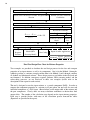
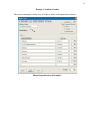
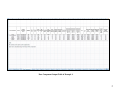
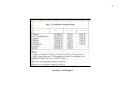
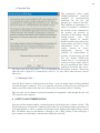
HMCRP
HAZARDOUS
MATERIALS
COOPERATIVE
RESEARCH
PROGRAM
REPORT 2
Sponsored by the
Pipeline and Hazardous
Materials Safety
Assessing Soil and
Groundwater Impacts
of Chemical Mixture Releases
from Hazardous Materials
Transportation Incidents
Administration
TRANSPORTATION RESEARCH BOARD 2010 EXECUTIVE COMMITTEE*
OFFICERS
CHAIR: Michael R. Morris, Director of Transportation, North Central Texas Council of Governments, Arlington
VICE CHAIR: Neil J. Pedersen, Administrator, Maryland State Highway Administration, Baltimore
EXECUTIVE DIRECTOR: Robert E. Skinner, Jr., Transportation Research Board
MEMBERS
J. Barry Barker, Executive Director, Transit Authority of River City, Louisville, KY
Allen D. Biehler, Secretary, Pennsylvania DOT, Harrisburg
Larry L. Brown, Sr., Executive Director, Mississippi DOT, Jackson
Deborah H. Butler, Executive Vice President, Planning, and CIO, Norfolk Southern Corporation, Norfolk, VA
William A.V. Clark, Professor, Department of Geography, University of California, Los Angeles
Eugene A. Conti, Jr., Secretary of Transportation, North Carolina DOT, Raleigh
Nicholas J. Garber, Henry L. Kinnier Professor, Department of Civil Engineering, and Director, Center for Transportation Studies, University of
Virginia, Charlottesville
Jeffrey W. Hamiel, Executive Director, Metropolitan Airports Commission, Minneapolis, MN
Paula J. Hammond, Secretary, Washington State DOT, Olympia
Edward A. (Ned) Helme, President, Center for Clean Air Policy, Washington, DC
Adib K. Kanafani, Cahill Professor of Civil Engineering, University of California, Berkeley
Susan Martinovich, Director, Nevada DOT, Carson City
Debra L. Miller, Secretary, Kansas DOT, Topeka
Sandra Rosenbloom, Professor of Planning, University of Arizona, Tucson
Tracy L. Rosser, Vice President, Corporate Traffic, Wal-Mart Stores, Inc., Mandeville, LA
Steven T. Scalzo, Chief Operating Officer, Marine Resources Group, Seattle, WA
Henry G. (Gerry) Schwartz, Jr., Chairman (retired), Jacobs/Sverdrup Civil, Inc., St. Louis, MO
Beverly A. Scott, General Manager and Chief Executive Officer, Metropolitan Atlanta Rapid Transit Authority, Atlanta, GA
David Seltzer, Principal, Mercator Advisors LLC, Philadelphia, PA
Daniel Sperling, Professor of Civil Engineering and Environmental Science and Policy; Director, Institute of Transportation Studies; and Interim
Director, Energy Efficiency Center, University of California, Davis
Kirk T. Steudle, Director, Michigan DOT, Lansing
Douglas W. Stotlar, President and CEO, Con-Way, Inc., Ann Arbor, MI
C. Michael Walton, Ernest H. Cockrell Centennial Chair in Engineering, University of Texas, Austin
EX OFFICIO MEMBERS
Peter H. Appel, Administrator, Research and Innovative Technology Administration, U.S.DOT
J. Randolph Babbitt, Administrator, Federal Aviation Administration, U.S.DOT
Rebecca M. Brewster, President and COO, American Transportation Research Institute, Smyrna, GA
George Bugliarello, President Emeritus and University Professor, Polytechnic Institute of New York University, Brooklyn; Foreign Secretary,
National Academy of Engineering, Washington, DC
Anne S. Ferro, Administrator, Federal Motor Carrier Safety Administration, U.S.DOT
LeRoy Gishi, Chief, Division of Transportation, Bureau of Indian Affairs, U.S. Department of the Interior, Washington, DC
Edward R. Hamberger, President and CEO, Association of American Railroads, Washington, DC
John C. Horsley, Executive Director, American Association of State Highway and Transportation Officials, Washington, DC
David T. Matsuda, Deputy Administrator, Maritime Administration, U.S.DOT
Victor M. Mendez, Administrator, Federal Highway Administration, U.S.DOT
William W. Millar, President, American Public Transportation Association, Washington, DC
Tara O’Toole, Under Secretary for Science and Technology, U.S. Department of Homeland Security, Washington, DC
Robert J. Papp (Adm., U.S. Coast Guard), Commandant, U.S. Coast Guard, U.S. Department of Homeland Security, Washington, DC
Cynthia L. Quarterman, Administrator, Pipeline and Hazardous Materials Safety Administration, U.S.DOT
Peter M. Rogoff, Administrator, Federal Transit Administration, U.S.DOT
David L. Strickland, Administrator, National Highway Traffic Safety Administration, U.S.DOT
Joseph C. Szabo, Administrator, Federal Railroad Administration, U.S.DOT
Polly Trottenberg, Assistant Secretary for Transportation Policy, U.S.DOT
Robert L. Van Antwerp (Lt. Gen., U.S. Army), Chief of Engineers and Commanding General, U.S. Army Corps of Engineers, Washington, DC
*Membership as of October 2010.
HAZARDOUS MATERIALS COOPERATIVE RESEARCH PROGRAM
HMCRP REPORT 2
Assessing Soil and
Groundwater Impacts
of Chemical Mixture Releases
from Hazardous Materials
Transportation Incidents
Richard G. Lewis
Ziqi He
HSA ENGINEERS & SCIENTISTS
A Member of the Conestoga-Rovers & Associates
Family of Companies
Fort Myers, FL
Subscriber Categories
Highways • Motor Carriers • Railroads • Environment • Freight Transportation
Geotechnology • Hydraulics and Hydrology
Research sponsored by the Pipeline and Hazardous Materials Safety Administration
TRANSPORTATION RESEARCH BOARD
WASHINGTON, D.C.
2010
www.TRB.org
HAZARDOUS MATERIALS COOPERATIVE
RESEARCH PROGRAM
HMCRP REPORT 2
The safety, security, and environmental concerns associated with
transportation of hazardous materials are growing in number and
complexity. Hazardous materials are substances that are flammable,
explosive, or toxic or that, if released, produce effects that would threaten
human safety, health, the environment, or property. Hazardous materials
are moved throughout the country by all modes of freight transportation,
including ships, trucks, trains, airplanes, and pipelines.
The private sector and a diverse mix of government agencies at all levels
are responsible for controlling the transport of hazardous materials and for
ensuring that hazardous cargoes move without incident. This shared goal
has spurred the creation of several venues for organizations with related
interests to work together in preventing and responding to hazardous
materials incidents. The freight transportation and chemical industries;
government regulatory and enforcement agencies at the federal and state
levels; and local emergency planners and responders routinely share
information, resources, and expertise. Nevertheless, there has been a longstanding gap in the system for conducting hazardous materials safety and
security research. Industry organizations and government agencies have
their own research programs to support their mission needs. Collaborative
research to address shared problems takes place occasionally, but mostly
occurs on an ad hoc basis.
Acknowledging this gap in 2004, the U.S. DOT Office of Hazardous
Materials Safety, the Federal Motor Carrier Safety Administration, the
Federal Railroad Administration, and the U.S. Coast Guard pooled their
resources for a study. Under the auspices of the Transportation Research
Board (TRB), the National Research Council of the National Academies
appointed a committee to examine the feasibility of creating a cooperative
research program for hazardous materials transportation, similar in concept
to the National Cooperative Highway Research Program (NCHRP) and the
Transit Cooperative Research Program (TCRP). The committee concluded,
in TRB Special Report 283: Cooperative Research for Hazardous Materials
Transportation: Defining the Need, Converging on Solutions, that the need for
cooperative research in this field is significant and growing, and the
committee recommended establishing an ongoing program of cooperative
research. In 2005, based in part on the findings of that report, the Safe,
Accountable, Flexible, Efficient Transportation Equity Act: A Legacy for
Users (SAFETEA-LU) authorized the Pipeline and Hazardous Materials
Safety Administration (PHMSA) to contract with the National Academy of
Sciences to conduct the Hazardous Materials Cooperative Research Program
(HMCRP). The HMCRP is intended to complement other U.S. DOT
research programs as a stakeholder-driven, problem-solving program,
researching real-world, day-to-day operational issues with near- to midterm time frames.
Project HM-06
ISSN 2150-4849
ISBN: 978-0-309-15527-4
Library of Congress Control Number 2010941499
© 2010 National Academy of Sciences. All rights reserved.
COPYRIGHT INFORMATION
Authors herein are responsible for the authenticity of their materials and for obtaining
written permissions from publishers or persons who own the copyright to any previously
published or copyrighted material used herein.
Cooperative Research Programs (CRP) grants permission to reproduce material in this
publication for classroom and not-for-profit purposes. Permission is given with the
understanding that none of the material will be used to imply TRB, AASHTO, FAA, FHWA,
FMCSA, FTA, RITA, or PHMSA endorsement of a particular product, method, or practice.
It is expected that those reproducing the material in this document for educational and notfor-profit uses will give appropriate acknowledgment of the source of any reprinted or
reproduced material. For other uses of the material, request permission from CRP.
NOTICE
The project that is the subject of this report was a part of the Hazardous Materials
Cooperative Research Program, conducted by the Transportation Research Board with the
approval of the Governing Board of the National Research Council.
The members of the technical panel selected to monitor this project and to review this
report were chosen for their special competencies and with regard for appropriate balance.
The report was reviewed by the technical panel and accepted for publication according to
procedures established and overseen by the Transportation Research Board and approved
by the Governing Board of the National Research Council.
The opinions and conclusions expressed or implied in this report are those of the
researchers who performed the research and are not necessarily those of the Transportation
Research Board, the National Research Council, or the program sponsors.
The Transportation Research Board of the National Academies, the National Research
Council, and the sponsors of the Hazardous Materials Cooperative Research Program do
not endorse products or manufacturers. Trade or manufacturers’ names appear herein
solely because they are considered essential to the object of the report.
Published reports of the
HAZARDOUS MATERIALS COOPERATIVE RESEARCH PROGRAM
are available from:
Transportation Research Board
Business Office
500 Fifth Street, NW
Washington, DC 20001
and can be ordered through the Internet at:
http://www.national-academies.org/trb/bookstore
Printed in the United States of America
COOPERATIVE RESEARCH PROGRAMS
CRP STAFF FOR HMCRP REPORT 2
Christopher W. Jenks, Director, Cooperative Research Programs
Crawford F. Jencks, Deputy Director, Cooperative Research Programs
William C. Rogers, Senior Program Officer
Charlotte Thomas, Senior Program Assistant
Eileen P. Delaney, Director of Publications
Ellen M. Chafee, Editor
Rachel Kirkland, Senior Editorial Assistant
HMCRP PROJECT 06 PANEL
Thomas Moses, Spill Center, Hudson, MA (Chair)
Craig Bartlett, DuPont Company, Wilmington, DE
Cheryl A. “Cherry” Burke, Dow Chemical Company, Midland, MI
Robert E. Fronczak, Association of American Railroads, Washington, DC
Zdenek “Zed” Hejzlar, Engineering Systems, Inc., Fort Myers, FL
John Walton, University of Texas - El Paso, El Paso, TX
Ryan F. Paquet, PHMSA Liaison
Christine Gerencher, TRB Liaison
AUTHOR ACKNOWLEDGMENTS
The research reported herein was performed under Dr. Richard G. Lewis, P.E., Principal at HSA Engineers & Scientists. Dr. Ziqi (Zeke) He, P.E., Environmental Engineer with HSA Engineers & Scientists, was
responsible for the thermodynamic calculation and design tool. William H. Hutchings, P.G., Professional
Geologist with HSA Engineers & Scientists and Ph.D. candidate at the University of South Florida, was
responsible for fate transport modeling. Gordon L. Walters, P.E., Environmental Engineer at HSA Engineers & Scientists, was responsible for the tool interface design. Kevin W. Worsham, Database Developer
with Conestoga-Rovers & Associates (CRA), and Julie Lidstone, Associate Database Manager with CRA,
were responsible for visual basic coding of the tool design. Doug Soutter, Hydrogeologist with CRA,
assisted with UNIFAC design. Dr. Hongze Gao, P.E., with CRA, assisted with the screening model design.
Ronald Foster, Senior Processing Engineer with CRA, assisted with the data and methodology collection.
In addition, the environmental department group at the office of HSA Engineers & Scientists in Fort
Myers, Florida, and the emergency response team at CRA’s office in Dallas, Texas, participated in data collection of chemical properties and the most commonly transported hazardous materials.
FOREWORD
By William C. Rogers
Staff Officer
Transportation Research Board
HMCRP Report 2: Assessing Soil and Groundwater Impacts of Chemical Mixture Releases
from Hazardous Materials Transportation Incidents presents a tool to assess, classify, predict,
and quickly communicate fate and transport characteristics of chemical mixtures released
into the soil and groundwater as a result of hazardous materials transportation incidents.
The tool was developed with a wide range of users in mind. For technical users, the property output table generates the fate and transport properties of an input mixture. For emergency response teams, it provides a quick review of the emergency response requirements
of a spill. For non-technical users, a color-coding function is included in the tool to compare the critical fate and transport properties to their pure chemical counterpart and highlight the key parameters affecting the mixture transport in the saturated and unsaturated
zones. The tool can also be used to determine whether shipping certain chemicals separately
or in mixtures will have significantly higher costs if an incident occurs and to estimate relative costs and timeframes of cleanup after an incident occurs.
Screening models, as well as detailed, computationally intensive models, exist to characterize site-specific impacts on soil and groundwater from hazardous materials releases.
These models require various fate and transport parameters as input, which are generally
available for pure chemical compounds. However, these parameters are typically unavailable for many of the commonly transported hazardous materials mixtures such as herbicides, paint, cleaning compounds, motor oil, antifreeze, gasoline, and ethanol.
Under HMCRP Project 06, HSA Engineers & Scientists was asked to (1) define and categorize the environmental hazards to soil and groundwater of pure chemicals and mixtures;
(2) identify sources and collect readily available data on fate and transport properties; (3)
develop a typology and identify and classify common solvents and mixtures that are likely
to be transported; (4) develop a typology to estimate the key parameters for different chemical mixtures; (5) design a tool to characterize, predict, and communicate the impact of
chemical mixtures in soil and groundwater environments and to estimate the fate and transport parameters of chemical mixtures released to soil and groundwater as a result of hazardous materials transportation incidents; (6) using the tool, estimate the fate and transport
parameters for 5 to 10 representative mixtures commonly transported and apply existing
basic screening models to estimate impact to soil and groundwater; and (7) refine the tool
to compare fate and transport characteristics of pure chemicals to chemical mixtures in
order to rank the relative impacts to soil and groundwater.
The chemical mixture tool, a user guide, and the contractor’s final report for HMCRP
Project 06 can be found on CRP-CD-90: Chemical Mixture Tool for HMCRP Report 2, which
is bound into this publication. For the convenience of readers, the research team’s Tool
Design Process Example (Appendix H) and the User Operational Manual (Appendix M)
are also provided herein.
CONTENTS
1
Summary
6
Contents of Contractor’s Final Report for HMCRP Project 06
(Final Report Contained on CRP-CD-90)
9
Appendix H Tool Design Process Example
32
Appendix M User Operational Manual
54
List of Acronyms and Symbols
1
SUMMARY
Assessing Soil and Groundwater Impacts of
Chemical Mixture Releases from Hazardous
Materials Transportation Incidents
Introduction
Each year, large quantities of hazardous materials are transported throughout the United
States. In the event of an incident or accident, these hazardous materials can be released
to the environment, thereby impacting soil and groundwater, leading to costly emergency
response and cleanup efforts. Many impact measurement techniques in use today concentrate on fatalities/injuries, property damage, and emergency impacts, but exclude environmental and ecological impacts associated with releases into soil, groundwater, aquatic
features, or natural habitats. Consequently, risk management decisions are being made in
the absence of the comprehensive information necessary to mitigate long-term environmental risk. The screening model developed in this research is meant to aid in addressing
this concern. As with all screening model requirements to assess the subsurface impact of
hazardous materials, chemical-specific fate and transport data, as well as site-specific
data, are necessary input parameters. While the fate and transport data are available for
pure chemicals, similar data are not usually available for mixtures of hazardous materials that
are commonly transported (e.g., herbicides, paint, cleaning compounds, motor oil, antifreeze,
gasoline, and ethanol).
The goal of this research was to develop a tool to estimate the critical fate and transport parameters of chemical mixtures for use in common fate and transport models,
allowing the user to efficiently and effectively compare and predict the potential impacts
of releases from transportation incidents. Specifically, the developed tool will assess, classify, predict, and quickly communicate fate and transport characteristics of chemical
mixtures released into the soil and groundwater as a result of hazardous materials transportation incidents.
The research team has completed 16 months of research on HMCRP Project 06, “Soil and
Groundwater Impacts of Chemical Mixture Releases from Hazardous Materials Transportation Incidents.” A white paper submitted in June 2009 summarizes the preliminary efforts
(Phase I, Tasks 1 to 4 outlined in the contract):
•
Task 1—define and categorize the environmental hazards to soil and groundwater of pure
chemicals and mixtures,
• Task 2—identify sources and collect readily available data on fate and transport properties,
• Task 3—develop a typology and identify and classify common solvents and mixtures that
are likely to be transported by the industry and significantly control or alter the hazardous
material fate and transport properties, and
• Task 4—develop a typology to estimate the key parameters for different chemical mixtures.
2
In September 2009, the research team proceeded to implement Phase 2 (Tasks 5 through 8)
of the research project:
•
Task 5—design a tool to characterize, predict, and communicate the impact of chemical
mixtures in soil and groundwater environments and to estimate the fate and transport parameters of chemical mixtures released to soil and groundwater as a result of hazardous
materials transportation incidents;
• Task 6—use the tool to estimate the fate and transport parameters for 5 to 10 representative mixtures commonly transported and to apply existing basic screening models to
estimate impact to soil and groundwater;
• Task 7—refine the tool to compare fate and transport characteristics of pure chemicals versus chemical mixtures in order to rank the relative impacts to soil and groundwater; and
• Task 8—prepare a final report that fully explains the tool and documents the entire
research effort, explains and justifies recommendations, provides background information used in the development of recommendations that addresses deficiencies and
recommends further research.
Consistent with the contract scope, the research team designed the tool using the typology table collected in Phase I as the database and refined the tool using the selected mixtures
and existing screening models. The second phase of activity incorporated the data and opinions garnered in Phase I to develop the tool itself. This phase encompassed the design and
construction of the tool, and the application of the tool to provide estimates of fate and
transport values for several representative mixtures. The tool was then used to determine
the effect of changes in these fate-and-transport parameters on the impact to soil and
groundwater after a release. CRP-CD-90: Chemical Mixture Tool for HMCRP Report 2, provided with this publication, contains the chemical mixture tool, an operational manual for
the tool, and the team’s final research report for HMCRP Project 06.
Findings
The summary of the literature review and expert interviews is provided for the top-ranked
transported or spilled hazardous materials from the Spill Center; Association of American
Railroads (AAR); Commodity Flow Survey (CFS); Conestoga-Rovers & Associates emergency response team; and the analysis of the incident reports database search from the
Office of Hazardous Materials Safety in the U.S. DOT. Fuels and ethanol-blended fuels,
alcohols, acids and bases, paints and related materials are the dominant hazardous material
classes according to commodity transported and incidents reported. As identified in the
interviews and literature review, the most important mixture is gasoline and ethanol. No
clear second mixture was identified, although Not Otherwise Specified (NOS) mixtures
clearly make up a large volume of what is transported.
The research team has reviewed and assimilated numerous scientific articles and agency
reports regarding chemical fate and transport and the methods for estimating the properties
of mixtures, including Raoult’s Law, Universal Functional Activity Coefficient (UNIFAC),
Cosolvency Effect, and Linear Solvation Energy Relationship (LSER). The approach to estimate the properties of chemical mixtures and the design of a tool have been provided for
both ideal and non-ideal chemical mixtures. Considering that UNIFAC has been more versatile over other methods since it works for various solution systems, including those with
high nonideality, the research team built a Microsoft Excel UNIFAC (xlUNIFAC) to function as the basis of the chemical mixture tool. This feature is a major strength of UNIFAC and
is extremely valuable in estimating solubility of hydrophobic environmental contaminants
3
in multiple-component systems, which are very difficult to characterize experimentally. In
the scenarios where xlUNIFAC does not function for a chemical mixture due to the lack of
the molecular volume and surface area (i.e., Rk and Qk) or the group interaction parameters
(i.e., anm), the cosolvent effects were incorporated into the tool as a second module to estimate the solubilities of chemicals in case of the presence of major cosolvents.
A chemical mixture tool was developed to estimate the fate and transport properties of
chemical mixtures using the xUNIFAC model, Raoult’s Law, and the Cosolvency—Log Kow
Model. The tool is capable of modeling a mixture containing up to 29 components. Approximately 530 chemicals have UNIFAC group assignments, and the linear free energy relationships (LFERs) between the cosolvency power and log Kow are included for 15 completely
water-miscible solvents, which are often used in industrial and environmental activities. The
output table of the tool consists of the following: (1) chemical identification (name, CAS#,
molecular weight), hazardous information (U.S. DOT Hazardous Class and UN/NA#);
(2) mixture characteristics (mass percent, volume percent, mole fraction); and (3) physical
chemical properties for the input mixture and its components (water solubility, vapor pressure, surface tension, viscosity, partitioning among mixture/water/air, partitioning between
water and organic carbon/octanol, diffusion coefficients in air/water/mixture, and half-life
time), which can be used to simulate the characteristics of non-aqueous phase liquid (NAPL)
(where applicable) in soil, water, and air.
In tests with 11 representative mixtures—including gasoline, methyl tertiary butyl ether
(MTBE)-blended gasoline, ethanol-blended gasoline, coal tar, paint, ink, lacquer thinner,
and drycleaner solvent—the tool has been versatile at estimating the fate and transport properties of hazardous mixtures. Hydrocarbon Spill Screening Model (HSSM), Multiphase
Flow and Multicomponent Transport Model (MOFAT), and BIOSCREEN-AT are used as
screening models to simulate the fate and transport of selected mixtures in subsurface. Benzene, toluene, ethylbenzene and xylene (BTEX), particularly benzene, was selected as the
target compound to analyze the impact of ethanol and MTBE on gasoline based on the
equivalent spill scenarios of oxygenate-free gasoline because benzene is the most mobile
gasoline-derived contaminant that possesses significant toxicity and groundwater impact.
Results indicated that the presence of 20% ethanol may cause a benzene plume in groundwater to be 30% longer than that in equivalent gasoline under anaerobic conditions, while
there were no significant changes in benzene transport under aerobic biodegradation. The
MTBE addition to gasoline does not significantly affect the gasoline component transport.
However, the effect of MTBE itself on the environment is a concern due to MTBE’s high
water solubility and low biodegradation under both aerobic and anaerobic conditions.
Conclusions
The chemical mixture tool was developed with a wide range of users in mind. For highly
technical users, the property output table generates the fate and transport properties of an
input mixture. For emergency response teams, the emergency response guide provides a
quick review of the emergency response to a spill. For non-technical users, a color-coding
function is included in the tool to compare the critical fate and transport properties to their
pure chemical counterparts and highlight the key parameters affecting the mixture transport
in the unsaturated (i.e., vadose) zone. A simplified version of Domenico’s model, designed
by the research team, is included to simulate chemical fate and transport in groundwater.
Without the availability of external screening models, the research team screening model can
be applied directly to simulate the transport of a hazardous mixture in groundwater.
Tool comparison, calibration, sensitivity analysis, and uncertainty analysis showed that
the tool estimates mixture properties (e.g., interfacial tension and viscosity) within a mean
4
error of 30% and the NAPL-water interface properties (e.g., solubility and partition coefficient) within a maximum factor of 5.0, which is relatively small compared with the imprecise
knowledge of subsurface gasoline release volumes and scenarios. When data are not available, this tool can be utilized to estimate the properties of a mixture.
The tool results can be used to determine whether shipping certain chemicals separately
or in mixtures will have significantly higher costs if an incident occurs, aiding in the emergency planning costs. The tool results can be used to estimate the relative costs and timeframes of cleanup after an incident occurs. The tool can also be used by remediation engineers to provide better remediation alternatives, given the availability of different properties
of mixtures versus pure chemicals. For example, regulators and scientists could use the tool
to estimate the properties of novel additives in future fuel formulations and thereby provide
key inputs for determining the transportation facility upgrade and assessing environmental
transport of these compounds using external screening models.
Tool Limitations and Future Research Recommendations
The main limitation of the tool is that it cannot be used for all chemical substances contained in the database of approximately 740 components derived from literary research and
interviews with professional personnel based on hazardous material classification and commodity flow survey and incident reports. That said, data for new chemicals can be added as
pure-phase information becomes available. The intended application domain is for liquid
organic chemicals, particularly petroleum and related compounds. Inorganic and organometallic chemicals generally are outside the tool’s domain. Future work may be focused on the expansion of the typology table database to a larger database to simulate mixtures that consist
of more chemicals. In addition, further research is needed to update the xlUNIFAC parameters with the latest available data. For example, as the largest database, the commercial
UNIFAC still lacks parameters for some halogenated compounds and new pharmaceutical
compounds.
This study is focused on the mixture source zone property estimate. Therefore, the chemical property parameters were calculated based on the assumption that the NAPL and
groundwater reach equilibria for individual components. The kinetic process of the interaction zone was not considered, and the interaction between the NAPL source zone and the
dissolved plume in groundwater was not modeled in this study. For example, half-life time
was produced by the tool for anaerobic and aerobic conditions from the typology table,
which does not represent site-specific decay. Although the tool generates property parameters with a factor of 5.0, field assessment is necessary to further calibrate the tool for modification to simulate the field spill scenarios. The tool will not be able to assess the property
changes with the temporal NAPL composition changes or the decay in the downgradient
groundwater. For example, the rapid transfer of ethanol from gasoline into the water in the
vadose zone (e.g., small volume spills) may not change the gasoline bulk transport properties (e.g., interfacial tension and viscosity) as predicted in this study. Furthermore, the quick
degradation of ethanol in the groundwater will alter the cosolvency power, as well as the
biodegradation of other components. Improved tool modification is required to integrate
the mixture degradation in the field, especially the ethanol effect on the biodegradation of
BTEX in the downgradient of the plumes.
A screening model has been incorporated within the tool for the users to simulate the fate
and transport in groundwater. However, the screening model results by HSSM and MOFAT
indicate that the mixtures have dramatically different transport in the unsaturated zone due
to changes in the density, interfacial tension, and viscosity. The behavior of the mixture in
the unsaturated zone will significantly affect the groundwater fate and transport. Therefore,
5
combined with the existing groundwater model, further research is necessary to design a vadose zone screening model to simulate the mixture fate in subsurface based on the spill scenarios (e.g., spill volume, mixture component, and site-specific hydrogeologic setting). A
user-friendly unit conversion may be included within the tool to export the tool results directly
to the required form of screening models.
Although the color-coding function is designed in the tool to compare the fate and transport characteristics of pure chemicals versus chemical mixtures in order to rank the relative
impacts to soil and groundwater, future research is needed to compare the concentrations
in subsurface to EPA clean up levels and to consider the cost and time frame of active remediation compared to natural attenuation. This module may be designed to estimate the cost
of the most commonly used remedial approaches (e.g., groundwater pump-treat, air sparging, soil vapor extraction, chemical oxidation, and enhanced natural attenuation) at different
time frames after the incident spills.
The current version of the chemical mixture tool, provided on CRP-CD-90, was designed
and tested to work with the PC version of Microsoft Excel. Additional research may be
needed to modify the tool to work with a Mac system.
6
Contents of Contractor’s Final
Report for HMCRP Project 06
(Final Report Contained on CRP-CD-90)
LIST OF TABLES .......................................................................................................... iv
LIST OF FIGURES ........................................................................................................ vi
LIST OF ACRONYMS AND SYMBOLS ...................................................................... viii
ABSTRACT .................................................................................................................... xi
AUTHOR ACKNOWLEDGEMENTS ............................................................................ xi
EXECUTIVE SUMMARY ......................................................................................... ES-1
CHAPTER 1. INTRODUCTION...................................................................................... 1
1.1
1.2
BACKGROUND .............................................................................................................. 1
SCOPE OF WORK .......................................................................................................... 2
CHAPTER 2. RESEARCH APPROACHES ..................................................................... 5
2.1
PHASE I APPROACHES ................................................................................................ 5
2.1.1
Task 1 Literature Review and Expert Interview ....................................................... 5
2.1.2
Task 2 Identify Data Sources and Collect Readily Available Data .......................... 7
2.1.2.1
External Electronic and Text Databases ............................................................ 7
2.1.2.2
Existing Software .............................................................................................. 8
2.1.2.3
Thermodynamic Calculation of Pure Chemicals ............................................... 8
2.1.2.4
Properties of Chemical Mixture ........................................................................ 8
2.1.3
Task 3 Tool Design Conceptual Model .................................................................... 8
2.1.3.1
“Lump” Component .......................................................................................... 8
2.1.3.2
Ideal Chemical Mixtures ................................................................................. 10
2.1.3.2.1 Solubility (Sm) of Chemical Mixture in Aqueous Phase..............................11
2.1.3.2.2 Effective Vapor Pressure (Pm) of Chemical Mixture ...................................11
2.1.3.2.3 Other Properties of Chemical Mixture..........................................................11
2.1.3.2.4 Partitioning between Chemical Mixture and Water Air Soil Phases ...........13
2.1.3.2.5 Degradation of Mixture Source (km) ............................................................14
2.1.3.3
Non-Ideal Chemical Mixtures ......................................................................... 14
2.1.3.3.1 Activity Coefficient in a Mixture Phase ......................................................15
2.1.3.3.2 Partitioning between Chemical Mixture and Water Air Soil Phases ...........15
2.1.3.3.3 Co-solvency Effect in Aqueous Phase .........................................................16
2.1.3.3.4 Salinity and pH Effect in Aqueous Phase ....................................................17
2.1.3.3.5 Effective Solubility (Sm) and Vapor Pressure (Pm) of Chemical Mixture ...18
2.1.3.3.6 Other Properties of Chemical Mixture.........................................................18
7
2.1.3.4
Review of Screening Models........................................................................... 18
2.1.3.5
Preliminary Design of the Tool and Communications .................................... 19
2.2
PHASE II APPROACHES............................................................................................. 21
2.2.1
Task 5 Chemical Mixture Tool (CMT) Design ...................................................... 69
2.2.1.1
Module 1 xlUNIFAC ....................................................................................... 69
2.2.1.1.1 Theoretical Background ...............................................................................69
2.2.1.1.2 Evaluation of xlUNIFAC .............................................................................77
2.2.1.2
Module 2 Cosolvency-Log Kow Model ........................................................... 78
2.2.1.2.1 Theoretical Background ...............................................................................78
2.2.1.2.2 Co-solvency power and log Kow Correlation Parameters ............................79
2.2.1.3
Module 3 Raoult’s Law ................................................................................... 80
2.2.1.4
Chemical Mixture Tool (CMT) Development................................................. 80
2.2.1.4.1 Input Interface ..............................................................................................81
2.2.1.4.2 Output Interface ...........................................................................................82
2.2.1.4.3 Example of Chemical Mixture Tool (CMT) Design....................................83
2.2.1.5
Emergency Response Guidance ...................................................................... 84
2.2.1.6
Modified Domenico Model ............................................................................. 84
2.2.1.6.1 Domenico Analytical Model Equation ........................................................84
2.2.1.6.2 Graphical Interface and Data Entry .............................................................85
2.2.1.6.3 Comparison to Existing Screening Models..................................................91
2.2.1.6.4 Graphical Plume Output and Application ....................................................92
2.2.1.6.5 Troubleshooting ...........................................................................................93
2.2.2
Task 6 Estimate the Fate and Transport Parameters for Representative Mixtures . 94
2.2.2.1
Representative Mixtures .................................................................................. 94
2.2.2.2
Tool Results of Representative Mixtures.......................................................... 94
2.2.2.3
Fate and Transport Modeling of Representative Mixtures ............................ 104
2.2.2.3.1 HSSM Simulation Results .........................................................................105
2.2.2.3.2 MOFAT Simulation Results ......................................................................116
2.2.2.3.3 BIOSCREEN-AT Simulation Results .......................................................130
2.2.2.4
Comparison and Analysis of Transport Properties and Simulation
Characteristics.................................................................................................134
2.2.2.4.1 Analysis of HSSM Results for Gasoline....................................................134
2.2.2.4.2 Analysis of MOFAT Results for Gasoline.................................................143
2.2.2.4.3 Analysis of BIOSCREEN-AT Results for Gasoline..................................148
2.2.2.4.4 Summary of Screening Model Analysis ....................................................150
2.2.3
Task 7 and Task 8 Tool Refinement and Report .................................................. 151
2.2.3.1
Chemical Mixture Tool (CMT) Evaluation and Calibration ......................... 151
2.2.3.1.1 Viscosity Comparison ................................................................................152
2.2.3.1.2 Interfacial Tension Comparison.................................................................153
2.2.3.1.3 Partition Coefficient of BTEX into Water from Gasoline .........................154
2.2.3.1.4 Calibration and Verification of Total Effective Solubility ........................155
2.2.3.2
Sensitivity and Uncertainty Analysis of Chemical Mixture Tool (CMT) ..... 157
2.2.3.2.1 Sensitivity Analysis ...................................................................................157
2.2.3.2.2 Uncertainty Analysis..................................................................................159
2.2.3.3
Color Coding and Property Ranking ............................................................. 162
8
CHAPTER 3. FINDINGS AND APPLICATIONS ........................................................ 163
3.1
3.2
3.3
TYPOLOGY TABLE .................................................................................................. 163
CHEMICAL MIXTURE TOOL DESIGN AND APPLICATION.............................. 164
FATE AND TRANSPORT OF ETHANOL-BLENDED GASOLINE....................... 164
CHAPTER 4. CONCLUSIONS AND RECOMMENDATIONS .................................... 165
4.1
4.2
CONCLUSIONS.......................................................................................................... 165
LIMITATIONS AND FURTHER RESEARCH RECOMMENDATIONS................ 165
REFERENCES ............................................................................................................ 168
Appendix A. Interview Questionnaire and Interview List.......................................................... A-1
Appendix B. Collected Chemical Properties .............................................................................. B-1
Appendix C. Top-Ranked Hazardous Materials Reported for Incidents or Transported ........... C-1
Appendix D. Major UN# NOS Hazardous Materials ................................................................. D-1
Appendix E. Review of Screening Models..................................................................................E-1
Appendix F. Classification of Hazardous Materials Transported...............................................F-1
Appendix G. Evaluating UNIFAC, Cosolvency and LSER Methods ........................................ G-1
Appendix H. Tool Design Process Example............................................................................... H-1
Appendix I. Synthetic Gasoline and Retail Gasoline Compositions ............................................I-1
Appendix J. HSSM Simulation Results ....................................................................................... J-1
Appendix K. MOFAT Simulation Results.................................................................................. K-1
Appendix L. BIOSCREEN-AT Simulation Results ....................................................................L-1
Appendix M. User Operational Manual..................................................................................... M-1
9
APPENDIX H
Tool Design Process Example
10
Mixture Input (Temperature and Volume, Weight or Mole Fraction)
Raoult's Law Conversion of Volume, Weight and Mole
Fraction
xlUNIFAC Evaluation
Yes
Module 1 xlUNIFAC
Reiteration Between mixture and Water till
Fi , mw , n+1 − F i , mw , n
Fi , mw , n
× 100 ≤ 5%
Estimate Viscosity, Diffusion
Coefficients
No
Module 2 or 3
Presence of Cosolvents
Yes
No
Module 2
Module 3
Cosolvency-Log K ow Raoult's
Law
Model
Output of Mixture and Component Properties
Emergency
Response
Guidance
Fate & Transport
Model (HSA
Screening Model)
Color Coding
Export for other Applications
Fate Model
Upgrade Regulator
Equipment Decision
Final Tool Design Flow Chart for Mixture Properties
Two examples are provided to elucidate the tool design process for the fate and transport
properties of an input mixture as well as its components. One is for the Module 1 through a
synthetic gasoline as a mixture example and the other is for Module 2 and 3 through a mixture
of alcohols and chlorinated solvents. These design processes are hidden in the final tool and
not formatted. In addition, emergency response guidance, HSA screening model, and the
color-coding processes are not discussed in these two examples (details refer to the
descriptions in the report for each section).
The tool is designed to run the input mixture as a pseudo component NAPL. In order to
compare the component properties in a mixture to its pure phase, the tool will also run each
individual component as a 100% input. Shown below are the output table of the mixture and
the pure components. Clearly, there are many calculation worksheets to obtain these final
output tables. The number of the calculation step depends on the input mixture properties.
Each step is provided below with notes of the calculation process beneath the tables
(Equations are provided in the report).
11
Example 1. Synthetic Gasoline
The mixture components and the mass fractions are shown in the Input Interface below.
Mixture Input Interface of Example 1.
12
Output Table of Example 1.
Pure Component Output Table of Example 1.
13
14
Tool Step 1 of Example 1.
Tool Step 2_1 of Example 1.
15
16
Tool Step 2_2 of Example 1.
Tool Step 3_1 of Example 1.
17
18
Tool Step 3_2 of Example 1.
Tool Step 3_1(2) of Example 1.
19
20
Tool Step 3_2(2) of Example 1.
Tool Step 3_2(Final) of Example 1.
21
22
Tool Step 3_1(3) of Example 1.
Tool Step 3_1(4) of Example 1.
23
24
Tool Step 3_1(Final) of Example 1.
Example 2. Chlorinated Solvents
The mixture components and the mass fractions are shown in the Input Interface below.
Input Interface of Example 2.
25
26
Output Table of Example 2.
Pure Component Output Table of Example 2.
27
28
Step 1 of Example 2.
Step 2_1 of Example 2.
29
30
Step 2_2 of Example 2.
Step 3_1 of Example 2.
31
32
APPENDIX M
User Operational Manual
33
TABLE OF CONTENTS
1.
Requirements...................................................................................................................34
2.
Starting the Program ......................................................................................................34
2.1.
2.2.
3.
Excel 2003 .....................................................................................................................34
Excel 2007 .....................................................................................................................35
Tool Input and Execution...............................................................................................36
3.1.
3.2.
3.3.
4.
Tool Input Parameters ...................................................................................................36
Reset the Tool................................................................................................................39
Running the Tool...........................................................................................................39
Output and Interpretation .............................................................................................39
4.1.
4.2.
4.3.
4.4.
5.
Color Coding .................................................................................................................40
Parameter Notes ............................................................................................................42
Screening Model ...........................................................................................................43
Emergency Response Guidebook (ERG 2008) .............................................................45
Troubleshooting ..............................................................................................................46
5.1.
5.2.
5.3.
5.4.
Adjusting Macro Security .............................................................................................46
Adding the ERROR Function for Screening Model .....................................................48
Spreadsheet-Related Problems ......................................................................................52
General ..........................................................................................................................53
34
1. REQUIREMENTS
− Excel (Program tested using versions 2003 and 2007)
− A Microsoft Windows PC (Currently not available in Mac)
− At least 256 MB of system RAM
− Recommended: 3.0+ Ghz CPU (2.0+ Ghz Parallel or Multi-core CPU)
2. STARTING THE PROGRAM
The tool is designed in Excel using Visual Basic for Application (VBA), requiring Excel Macros
to operate. Macros are written inside the tool to operate the toolbar buttons or help icons and
repeat the steps of common calculations.
2.1. Excel 2003
Depending on your macro security settings, you may see one of the following three messages
when you open the Excel file:
1)
2)
3)
35
If you see the first dialog box, please select the “Enable Macros” button and the tool will
initialize. The second and the third dialogue boxes will require you to reduce your security level
in Excel (Please see the troubleshooting section 5.1 for detailed assistance). Select the following:
“Menu,” then “Tools,” then “Options,” then “Security,” and then click on “Macro Security.”
Lower the security level to “Medium or Low.” This step requires that the user restart the Excel
Software and reopen the Chemical Mixture Tool.
Once the macro has been allowed to run according to the instructions above, the tool will show
the front page in Excel as shown below. Clicking the “RUN CMT” button will show the input
form and continue the tool process.
2.2. Excel 2007
Depending on your macro security settings, you may see the following warning when you open
the Excel file:
36
Click the “Options” button, and then choose the option: “Enable this content.” Click “Okay.” If
you do not see this item and did not receive the above warning, your security settings are too
strict (please refer to the troubleshooting section 5.1 for assistance).
Once the macro has been allowed to run per the above instructions, you should see the tool front
page in Excel as below. Clicking the “RUN CMT” button will show the input form and continue
the tool process.
3. TOOL INPUT AND EXECUTION
3.1. Tool Input Parameters
Interface and Help Button
37
On the Tool input interface, click the “Help” button on the right top corner and the Help menu
will open to illustrate the input interface functions as shown below.
1)
2)
3)
4)
5)
6)
7)
8)
9)
10)
Mixture Name: Enter the mixture name. The default is “Mixture, m.”
Temperature (Required): Enter the desired temperature.
Temperature Unit: Unit of associated temperature. Default is Kelvin.
Component Fraction: Method by which ratio of components will be defined.
Page Selection: Once a certain number of components have been entered,
additional pages will appear and can be toggled between here.
Component Input: Enter the component by either name or CAS number.
Ratio of Components: Based on (4), enter the amount of each component in the
mixture.
Function Buttons:
1.
Search: Allows a search of the registry by CAS or name (details below).
2.
Clear Selections: Resets the form.
3.
Run: Begins the calculation process and produces output.
Total: Displays the sum of (7). Must be 100 % by Mass or Volume; 1.0 by Molar
Fraction for the tool to proceed.
Reset Tool: Click to reset the tool at various mixture-water ratios.
38
11)
Help: Illustrate the Input Interface and functions.
Searching the Compound Registry
When the “Search” button is clicked on the main form, the above window will open. Using the
radio buttons, select which registry you would like to search. The drop down menu will allow
you to limit the way in which you search the registry to items which begin with your data entry,
items which end with your data entry, or items which contain your data entry at any point.
After completing it, click the “Search” button on this form, and results will be displayed (note:
entering nothing in the input box will result in all items in the registry being returned
alphanumerically).
To return a component to the main form, select
it from the resulting list and click the “Add to
Mixture” button. Only one anonym of a
chemical is in the tool database, therefore,
searching by CAS# will be the most convenient
means to find an input component.
If you do not see the component you are looking
for, you may use the “Clear” button to reset this
form and try again. If a desired chemical cannot
be found either by chemical name or CAS#
search, the desired chemical is not in the tool
database.
39
3.2. Reset the Tool
The nonaqueous phase liquid
(NAPL)-groundwater interfacial
equilibria are environmentally
significant for the fate and
transport of a solute in the field.
The solubility or partitioning of a
solute in a mixture is a function of
the fraction of the compound in
the mixture, the presence of
cosolvents in the mixture, and the
mixture-to-water
ratio.
For
example, ethanol in ethanolblended gasoline will partition into
aqueous phase and, only at certain
concentration levels (i.e., 5%
volume fraction in water),
subsequently
increase
the
solubility of hydrocarbons in
gasoline. Conservatively, the tool
sets the default NAPL-water
volume ratio as 1:1 to simulate the
scenarios of large volume spills or
the near contaminant zone, where
significant cosolvent may occur.
The actual ratio may range from 1:1 to 1:10 depending on the incident scenarios. Every time
when the tool is opened, it is automatically reset to a 1:1 ratio. Please enter the new ratio for
other cases.
3.3. Running the Tool
After the “Run” button is clicked on the main form, a series of simple checks will be performed
to ensure the input is complete. If it is, an action bar and series of status messages will appear to
inform you of the current action the tool is taking and to let you know that it is working.
This may take several minutes based on the number of components, path through the tool, and
CPU speed of your computer.
4. OUTPUT AND INTERPRETATION
After the tool has finished running, an output interface will be displayed as shown as below. The
default output page will provide a summary table of the fate and transport property parameters of
your input mixture as well as a number of calculated values further to the right of what is shown
here. In addition, there are four buttons (1 through 4) and a “Help” button (5) that will display a
basic summary of each button’s function from within the tool itself.
40
4.1. Color Coding
The "Color Coding” button (1) is designed to compare the properties of a component to its pure
phase using different colors. Clicking the button will toggle the color coding on and off. The
“Color Coding” button (1) will shade parameter Water Solubility through Anaerobic Half-Life
time based on the specific parameter in that column in the mixture compared to that same
parameter as a pure compound.
• The Lime Green color represents the ratio of the property less than 5.0, which indicates
that there are no significant changes in the property of the mixture compared to the pure
chemical.
• The Orange color represents the ratio of the property between 5.0 and 10.0, indicating
that there are slight changes in the property of the mixture compared to the pure
chemical.
• The Red color represents the ratio of the property greater than 10.0, indicating that the
chemical mixture may have a dramatic effect on the property of a component.
• The Blue color highlights the major mixture NAPL transport properties in the unsaturated
zone.
41
42
In addition, a note (shown above) will be added to each Orange/Red cell, which will show the
associated value when the compound is not mixed as well as the ratio between the two. It should
be noted that even though the color change from green to red indicates the severity of the
property change of a component in a mixture compared to its pure phase, the red color does not
guarantee the mixture is not acceptable considering the uncertainty of the tool.
4.2. Parameter Notes
The "Parameter Notes" button (2) is designed to interpret the physical and chemical parameters
and terms used in the output table. When this button is selected, a note box will open as below to
43
interpret the parameters and definitions in the output table. Click the “Return to Table” button to
return to the output interface.
4.3. Screening Model
The “Go to Component Plume” button (3) is designed to simulate a component plume in a
saturated groundwater aquifer with default hydrogeologic characteristics. Select any component
and then click the “Go to Component Plume” button and it will take the user to an interface of
the Domenico Analytical Model designed by the research team, where a plume of the component
is shown. The default simulation time is one year.
The “Return to Table” button below the plume illustration will return the user to the main output
sheet. Located to the right of the plume illustration are the entry parameters used to generate it.
These are the generic parameters, which can be adjusted to fit the specific conditions in question.
The concentration, partition coefficient, and half-life are calculated by the mixture tool (blue
borders with a red font) and should not be changed. Please use the “Help” button below the
input area to access detailed data entry instructions as shown below. Click the “Return to Plume”
button to return to the screening model interface.
44
45
4.4. Emergency Response Guidebook (ERG 2008)
The “Emergency Response Guide” button (4) is designed to assign each chemical component an
Emergency Response Guidebook (ERG 2008), which was developed by the United States
Department of Transportation (U.S. DOT). Select one component and click the “Emergency
Response Guide” button, and it will take the user to the interface of appropriate emergency
response guides according to the U.S. DOT Hazardous Class and United Nations Identification
Number (UN#) assigned to the component for proper shipping as shown below. Clicking the
“Return to Table” button at the bottom of the ERG will take the user to the current output
interface.
46
5. TROUBLESHOOTING
5.1. Adjusting Macro Security
Excel 2003:
From the menu, select “Tools” then “Options” to open the above screen. Select the Security Tab
from the groups at the top of this menu, and then click the “Macro Security” button from the
bottom of the Security Tab. This will open the following menu:
Here the user can change the security settings.
“Medium” is the recommended setting which
will result in the prompt mentioned above. A
higher security setting will not allow the tool to
run, and a lower security setting may allow
potentially malicious macros to run without
prompting, if the user is concerned.
Once this setting has been changed, the tool
must be closed and re-opened in order to
proceed.
47
Excel 2007:
Using the Office button (pictured to left) will show the following:
Here, the user will select the
highlighted button at the bottom
(Excel Options), which will allow
access to a number of application
settings.
On the next window, navigate first to
the “Trust Center” (1), and then open
the “Trust Center Settings” (2).
48
Finally, the user can change the security setting under “Macro Settings.” Selecting “Disable all
macros with notification” is recommended and will result in the same behavior described in this
document. Anything higher will prevent the tool from running, while anything lower will permit
potentially malicious macros to run without prompt.
Once this setting has been changed, the tool must be closed and re-opened in order to proceed.
5.2. Adding the ERROR Function for Screening Model
The tool will automatically turn on the Analysis Toolpak in Excel as an Add-in to run the
screening model. If it fails to turn on the ERROR Function in the Analysis Toolpak, a note will
show as pictured below. If this function is not available, the data source calculations for the
plume will result in “#VALUE!” Or “#NAME?” errors, and no chemical plume will be shown.
49
Next, install and load the Analysis ToolPak add-in following the instructions on the following
page.
Excel 2003:
From the menu, select “Tools” and then “Add-Ins” to open the second screen below. From this
menu, check the boxes next to both “Analysis ToolPak” and “Analysis ToolPak – VBA,” then
click OK. Close Excel and reopen it, then run the Chemical Mixture Tool; the issue associated
with the screening model plumes should be gone.
50
51
Excel 2007:
Using the Office button (pictured to left) will show the following:
Here, the user will select the highlighted button
at the bottom (Excel Options) which will allow
access to a number of application-wide settings.
Once the “Options” window is open, select the
“Add-Ins” tab on the right. This will display a
window which looks like the image below.
Select the “Go” button at the bottom of this
window.
52
The following menu will open. Simply check the boxes next to “Analysis ToolPak” and
“Analysis ToolPak – VBA,” then select “OK.” Close Excel and reopen it; then run the Chemical
Mixture Tool, and the issue associated with the screening model plumes should be gone.
5.3. Spreadsheet-Related Problems
The Tool was built in the Excel spreadsheet environment and spreadsheet-related problems may
occur for either the cell/table format or the component plume due to the calculation process.
Below are some anticipated problems and interpretations:
1) #### is displayed in a number box in the Output Table: The cell format is not compatible
with the value, (e.g., the number is too big to fit into the window). To fix this, select the
cell, pull down the format menu, select “Cells” and click on the “Number” tab. Change
the format of the cell until the value is visible. If the values still cannot be read, select the
format menu, select “Cells,” and click on the “Font” tab. Reduce the font size until the
value can be read.
2) #DIV/0! is displayed in the raw data for the screening model plume: The raw data for the
screening model is located in the bottom of the screening model interface. The most
common cause of this problem is that some input data in the screening model are missing.
In some cases, entering a zero in a box will cause this problem. Doublecheck to make
certain that all of the input cells required for your run have data. In addition, as described
in 5.2, the ERROR Function required for the Screening Model may cause this issue
(Please see the troubleshooting section 5.1 for detailed assistance).
53
3) The plume graphs seem to move around or change size: The screening model plume is
generated by Excel Standard Chart Wizard. This is a feature of Excel. When graph scales
are altered to accommodate different plotted data, the physical size of the graphs will
change slightly, sometimes resulting in a graph that spreads out over the fixed axis
legends. The research team has adjusted the graph scale (i.e., axis scale and the plume
display contours) according to the plume sizes. However, users still can manually resize
the graph to make it look nice again by double-clicking on the graph and resizing it (refer
to the Excel User’s Manual).
5.4. General
Most unexpected, abnormal behavior can be resolved by:
•
•
•
Restarting Excel,
Rebooting your computer, or
Returning to the original zipped document and re-extracting a fresh copy of the tool.
This tool’s main limitation is that it cannot be used for all chemical substances, with the database
of 740 components derived from literary research and interviews with professional personnel
based on hazardous material classification and commodity flow survey and incident reports. The
intended application domain is for liquid organic chemicals, particularly petroleum and related
compounds. Inorganic and organometallic chemicals generally are outside the tool’s domain. If
the desired chemical is out of the tool database, the current tool will not be able to generate the
property for the particular mixture and simulate the fate and transport in subsurface.
Detailed information concerning the development, performance, and application of the tool, as
well as the individual programs (e.g., Universal Functional Activity Coefficient (UNIFAC)
model, Raoult’s Law, and the Cosolvency-Log Kow Model) contained within it, can be found
within the theoretical section of the tool development manual. If there are any issues that are not
resolved by the manual, please contact HSA Engineers & Scientists at (239) 936-0789 or [email protected] .
54
LIST OF ACRONYMS AND SYMBOLS
AAR
API
ATSDR
BTEX
BTS
CAMEO
CAS #
CFS
CHEMTREC
DGAC
DNAPL
DOE
DOT
EAWAG
EPA
EPIWIN
FDEP
FGCU
HAZMAT
HMCRP
HSDB
HSSM
IAFC
IRIS
ISI
IUPAC
KOPT
LFER
LNAPL
LSER
LSST
MHMI
MIT
MOFAT
MSDS
NAPL
Association of American Railroads
American Petroleum Institute
Agency for Toxic Substances & Disease Registry
benzene, toluene, ethylbenzene, and xylene
Bureau of Transportation Statistics
Computer-Aided Management of Emergency Operations
Chemical Abstract Service registry number, which is unique identification
for chemicals. It is also referred to as CAS RN.
Commodity Flow Survey
Chemical Transportation Emergency Center
Dangerous Goods Advisory Council
Dense Non-aqueous Phase Liquid
U.S. Department of Energy
U.S. Department of Transportation
Swiss Federal Institute for Environmental Science and Technology
U.S. Environmental Protection Agency
Estimation Program Interface Suite
Florida Department of Environmental Protection
Florida Gulf Coast University
Hazardous Materials
Hazardous Materials Cooperative Research Program
Hazardous Substance Data Bank
Hydrocarbon spill screening model
International Association of Fire Chiefs
Integrated Risk Information System
Institute for Scientific Information
International Union of Pure and Applied Chemistry
Kinematic Oily Pollutant Transport
Linear Free Energy Relationship
Light non-aqueous phase liquids
Linear Solvation Energy Relationship
Linear Solvation Strength Theory
Managing Hazardous Materials Incident
Massachusetts Institute of Technology
Multiphase Flow & Multicomponent Transport Model
Material Safety Data Sheets
Non-aqueous Phase Liquid
55
NIST
NOS
NTSB
OPP
TRB
TSG
UN/NA #
Aerobic t1/2
Anaerobic t1/2
Da
Dw
Dm
foc
I
K
Ki, am
Ki, aw
Ki, mw
Ki, oc
Kow
MW
ρ
σ
σow
P
S
η
σi,j
γ
Cs
C0
αx
αy
αz
λ
ks
θe
θ−
R
National Institute of Standards and Technology
Not Otherwise Specified
National Transportation Safety Board
Office of Pesticide Programs
Transportation Research Board
Transient Source Gaussian Plume
United Nations or North American Identification Numbers
The half-life time of a component under aerobic conditions. The smaller
the half-life time, the faster the chemical decay.
The half life time of a component under anaerobic conditions
Diffusion coefficient in air
Diffusion coefficient in water
Diffusion coefficient in mixture
Fraction organic carbon
Hydraulic gradient (ft/ft)
Hydraulic conductivity (ft/yr)
Partition coefficient between air and the mixture, which is relevant for
phase equilibrium and the concentration in air
Partition coefficient between air and water (unitless)
Partition coefficient between the mixture and water, which is relevant for
phase equilibrium and the solubility in water
Partition coefficient of a component between organic carbon and water,
which is relevant for adsorption of a NAPL to sediment and the retardation
factor of a NAPL travel velocity
Partition coefficient between octanol and water
Molecular weight of the component, which is unique for each chemical
Density
Surface tension of a NAPL against air
The interfacial tension between the mixture and water
Vapor Pressure
The solubility in water
Dynamic viscosity
As the co-solvency power of the solvent for the compound i in co-solvent j
Activity Coefficient
Concentration in Source Zone (mg/L)
Concentration in Source Zone at t=0 (mg/L)
Longitudinal groundwater dispersivity (ft)
Transverse groundwater dispersivity (ft)
Vertical groundwater dispersivity (ft)
First-order decay coefficient for dissolved contaminants (yr−1)
First-order decay term for source concentration (yr−1) (no decay for the
source concentration based on the assumption of continuous source plume)
Effective soil porosity
Soil total porosity
Constituent retardation factor
Abbreviations and acronyms used without definitions in TRB publications:
AAAE
AASHO
AASHTO
ACI–NA
ACRP
ADA
APTA
ASCE
ASME
ASTM
ATA
ATA
CTAA
CTBSSP
DHS
DOE
EPA
FAA
FHWA
FMCSA
FRA
FTA
HMCRP
IEEE
ISTEA
ITE
NASA
NASAO
NCFRP
NCHRP
NHTSA
NTSB
PHMSA
RITA
SAE
SAFETEA-LU
TCRP
TEA-21
TRB
TSA
U.S.DOT
American Association of Airport Executives
American Association of State Highway Officials
American Association of State Highway and Transportation Officials
Airports Council International–North America
Airport Cooperative Research Program
Americans with Disabilities Act
American Public Transportation Association
American Society of Civil Engineers
American Society of Mechanical Engineers
American Society for Testing and Materials
Air Transport Association
American Trucking Associations
Community Transportation Association of America
Commercial Truck and Bus Safety Synthesis Program
Department of Homeland Security
Department of Energy
Environmental Protection Agency
Federal Aviation Administration
Federal Highway Administration
Federal Motor Carrier Safety Administration
Federal Railroad Administration
Federal Transit Administration
Hazardous Materials Cooperative Research Program
Institute of Electrical and Electronics Engineers
Intermodal Surface Transportation Efficiency Act of 1991
Institute of Transportation Engineers
National Aeronautics and Space Administration
National Association of State Aviation Officials
National Cooperative Freight Research Program
National Cooperative Highway Research Program
National Highway Traffic Safety Administration
National Transportation Safety Board
Pipeline and Hazardous Materials Safety Administration
Research and Innovative Technology Administration
Society of Automotive Engineers
Safe, Accountable, Flexible, Efficient Transportation Equity Act:
A Legacy for Users (2005)
Transit Cooperative Research Program
Transportation Equity Act for the 21st Century (1998)
Transportation Research Board
Transportation Security Administration
United States Department of Transportation