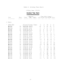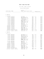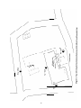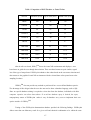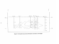
1
United States
Environmental Protection
Agency
Office of Research and
Development
Washington DC 20460
EPA/540/R-94/505
March 1994
GIS/KeyTM Envi ronmental
Data Management System
Innovative Technoloav
Evaluation Report
TECHNOLOGY EVALUATION
EPA/540/R-94/505
March 1994
GIS\KeyTM Environmental Data Management System
INNOVATIVE TECHNOLOGY EVALUATION REPORT
Risk Reduction Engineering Laboratory
Office of Research and Development
U.S. Environmental Protection Agency
Cincinnati, Ohio 45268
@ Printed on Recycled Paper
NOTICE
The information in this document has been prepared for the U.S. Environmental Protection
Agency’s (EPA) Superfund Innovative Technology Evaluation (SITE) Program under Contract No.
68-C0-0048. This document has been subjected to EPA’s peer and administrative reviews and has
been approved for publication as an EPA document. Mention of trade names or commercial products
does not constitute an endorsement or recommendation for use.
ii
FOREWORD
The Superfund Innovative Technology Evaluation (SITE) Program was authorized by the Superfund Amendments and Reauthorization Act (SARA) of 1986. The program is administered by the EPA
Office of Research and Development (ORD).. The purpose of the SITE Program is to accelerate the development and use of innovative cleanup technologies applicable to Superfund and other hazardous waste
sites. This purpose is accomplished through technology demonstrations designed to provide performance
and cost data on selected technologies.
This project consisted of an evaluation under the SITE Program of the GIS\KeyTM Environmental
Data Management System developed by GIS\Solutions, Inc. The software evaluation was conducted on
data typical of a Superfund site. The evaluation provided information on the performance and cost of the
software. This Innovative Technology Evaluation Report provides an interpretation of the data and
discusses the potential applicability of the software.
A limited number of copies of this report will be available at no charge from EPA’s Center for
Environmental Research Information, 26 West Martin Luther King Drive, Cincinnati, Ohio, 45268. Requests should include the EPA document number found on the report’s front cover. When the limited
supply is exhausted, additional copies can be purchased from the National Technical Information Service
(NTIS), Ravensworth Building, Springfield, Virginia, 22161, (703) 487-4600. Reference copies will be
available at EPA libraries in the Hazardous Waste Collection. You can also call the SITE Clearinghouse
hotline at (800) 424-9346 or (202) 382-3000 in Washington, D.C., to inquire about the availability of other
reports.
E. Timothy Oppelt, Director
Risk Reduction Engineering Laboratory
iii
TABLE OF CONTENTS
Section
Page
NOTICE .......................................... .........................................................................
FOREWORD .............................................................................................................
LIST OF TABLES ........................................................................................................
LIST OF FIGURES .......................................................................................................
ABBREVIATIONS ........................................................................................................
ACKNOWLEDGMENTS ...................... . . . . . . . . . . . . . . . . . . . . . . . . . . . . . . . . . . . . . . . . . . . . . . .. . . . . . . . . . . . .. . . . . . . . . . . . . .
EXECUTIVE SUMMARY ................................................................................................
ii
iii
vii
viii
x
xi
xii
1. Introduction ............................................................................................................
1
Background ..........................................................................................
Brief Description of Program and Reports . . . . . . . . . . . . . . . . . . . . . . . . . . . . . . . . . . . . . . . . . . . . . . . . . . .
Purpose of the ITER ................................................................................
Technology Description . . . . . . . . . . . . . . . . . . . . . . . . . . . . . . . . . . . . . . . . . . . . . . . . . . . . . . . . . . . . . . . . . . . . . . . . . . .
1
2
4
4
1.1
1.2
1.3
1.4
1.4.1
1.4.2
1.4.3
1.4.4
1.4.5
1.4.6
1.5
9
Boring Logs ..... . . . . . . . . . . . . . . . . . . . . . . . . . . . . . . . . . . . . . . . . . . . . . . . . . . . . . . . . . . . . . . . . . . . . . . . . . .
9
Structure Maps ...........................................................................
Geologic Cross Sections ................................................................. 9
Isopleth Maps ................................................................................................................ 9
Chemistry and Hydrology Graphs ............................................................................ 10
Tabular Reports ........................................................................................................... 11
Key Contacts ........................................................................................ .......................................
11
2. Software Application Analysis and Effectiveness ...........................................................................................................................................................................,
13
Background . . . . . . . . . . . . . ............................................................................................................................................................................................................................ .......
13
2.1
Key Features of the GIS\KeyTM Environmental Data Management System . . . . .
14
Methodology .................................................................................................................................................
16
2.1.1
2.2
2.2.1
2.3
Evaluation Results . . . . . . . . . . . . . .................................................................................................................................................................................................................
2.3.1
23.2
2.3.3
2.3.4
2.3.5
2.3.6
2.3.7
2.3.8
2.3.9
2.4
Test Data Set . . . . . . . . . . . . . . . . . . . . . . . . . . . . . ................................................................................................................................................................. . . . . . . . . 17
17
New Project Setup ...................................................................................................... 17
Data Entry ....................................................................................................................... 25
Data Checks, QA/QC
C Analysis, Updates, and Edits ........................................... 38
Data Processing ........................................................................................................... 44
Graphical Procedures ................................................................................................. 50
Products ........................................................................................................................ 77
Software Products vs. Reporting Requirements ................................................. 83
Hardware Considerations ........................................................................................ 9 6
System Training and Support ................................................................................. 100
References . . . . . . . . . . . . . . . . . . . . . . . . . . . . . . . . . . . . . . . . . . . . . . . . . . . . . . . . . . . . . . . . . . . . . . . . . . . . . . . . . . . . . . . . . . . . . . . . . . . . . . . . . . . . . . . . . . . . . . ........... .
V
106
TABLE OF CONTENTS (CONTINUED)
3.
Economic Analysis ............................................................................
3.1
3.2
3.3
3.4
Conclusions of EconomickAnalysis...................................................
Basis of Economic Analysis ...........................................................
Issues and Assumptions .............................................................
Results of Economic Analysis .......................................................
3.4.1
3.4.2
3.4.3
3.4.4
3.5
107
107
109
109
110
111
System and Accessories ..................................................... 110
Hardware and Support Software ..............................................
Labor ......................................................................... 112
Training and Maintenance ................................................... 112
References
........................................................................
116
y Requirements.....................................................................
4. OtherTechnology
117
Personnell Issues .....................................................................
117
5. Software Status .....................................................................................
119
Appendix I. Developer's Claims for GIS\KeyTM Software ................................................
121
4.1
I.1
Developer’s Claims, ....................................................................
121
Introduction ..................................................................
121
.
New Features of GIS\KeyTM Software ...............................................
121
I.1.1
1.2
y Database Modifications ................
Custom Boring Logs and Geology
Hydrology Database Modifications ...............................
Chemistry Database Changes and ITIR Reporting ..........................
GIS Utilities,, Menus, and Dialog Boxes .....................................
Stand-Alone
e Database Modifications .......................................
Improvements ...................................................
AutoCADD
Contouring PackageeImprovements .........................................
Third-Party Software Integration ...........................................
Data Security ................................................................
123
123
124
125
125
125
125
126
y Under Development ...............................
GIS\KeyTM Features Currently
126
1.2.1
I.2.2
I.2.3
1.2.4
I.2.5
I.2.6
I.2.7
I.2.8
I.2.9
I.3
Li3.1
I.3.2
I.3.3
13.4
Field Module ................................................................
Support of Multiple Databases ............................................. .
Air Module ..................................................................
Risk
k Module .................................................................
122
127
127
127
127
Summary ............................................................................
128
Appendix II. A Method for Determining Digitizing Accuracy GIS\KeyTM ...........................
131
I.4
LIST OF TABLES
Number
1
GIS\KeyTM Products ...............................................................................................................................
10
2
M ............................................................................................................
Items Evaluated for GIS\KeyTM
15
3
Historical Ranges Check ........................................................................................................................
39
4
Holding Time Check ...............................................................................................................................
40
5
Action Level Check .................................................................................................................................
42
6
Comparison of Well Elevation vs. Posted Values ............................................................................... 47
7
AutoCAD Supported Peripherals ........................................................................................................
74
8
Types of Contour Maps ..........................................................................................................................
80
9
Types of Graphs ......................................................................................................................................
84
10
Reporting Elements and Associated GIS\KeyTM Modules ...........................................................
97
11
Configurations and Peripherals ............................................................................................................
98
12
Recommended and Minimum Hardware Configurations for GIS\KeyTM Release 1.1.2 ..........
99
13
Selected Processing Times ......................................................................................................................
99
14
Project Data Management Costs, I-Year Basis ..................................................................................
108
15
GIS\KeyTM System and Accessory Costs ...........................................................................................
111
16
GIS\KeyTM Support Software ..............................................................................................................
113
17
Labor Requirements Using GIS\KeyTM .............................................................................................
113
18
Labor Requirements Using the Alternative System ......................................................................... 114
19
GIS\KeyTM Support Services ...............................................................................................................
Vii
115
LIST OF FIGURES
&i&?
Number
6
1
GIS\KeyTM Database Menu Structure ...................................................................................................
2
GIS\KeyTM Graphics Menu Structure
3
GIS\KeyTM Directory Structure
............................................................................................................
18
4
Example Map (Valdosta, GA Quadrangle) Provided by ADC in AutoCAD Drawing Format ......
20
5
GIS\KeyTM
M View Showing the Valdosta Airport and Geodetic Control Points .........................
22
6
.
Map Showing the Four Intermediate-zone Wells in the Intwells Symbol List.......................... 466
7
Posted Elevation (ft) Values for the Wells Selected to Build the Formation Structure Map.. .. 53
8
Geologic Structure Map Showing Grid and Contour Lines ........................................................... 54
9
6
Example Geologic Formation Structure Map ...... .............................................................................. 56
10
Example Geologic Formation Structure Map Showing the Results of Editing a Posted Value 57
11
Generation of a New Grid and Contour Lines Based on the Addition of Four Contour Control
...................................................................................................
Points .......................................................................................................................................................
12
8
58
Structure Map Reflecting New Contour Lines Generated from Original Data Points
Plus Four Contour Control Points .......................................................................................................
59
13
Contour Map of Benzene Concentration (mg/l)) Using Log QuickSurf. .....................................
60
14
Contour Map of Benzene Concentration (mg/l) Created Without Running Log QuickSurf......
61
15
Contour Map Produced with Log QuickSurf When a Well (MW-06A) Has a Concentration
Value of 0.................................................................................................................................................
63
16
Creating a Section Line B and B’ Across the Site ............................................................................... 65
17
Geologic Section (B-B’) Displaying Stick D a t a1 ..................................................................................... 66
18
Geologic Section (B-B’) Displaying Hatch Data ................................................................................. 67
19
GIS\KeyTM-provided Soil Hatch Patterns ..............................................................................................
20
Geologic Section (B-B’) Showing the Results of Changing the Hatch Scale Factor ................... 7 0
21
Soil Isopleth Cross-Section with Benzene Concentration Contours (mg/l) ................................ 71
22
3-Dimensional Orthographic Display of the Grid and Contour Lines Generated by
68
68
QuickSurf
f ................................................................................................................................................... 76
viii
viii
LIST OF FIGURES (CONTINUED)
m
Number
23
GIS\KeyTM Map Symbols ........................................................................................................................
24
Plot of Concentration vs. Time for Benzene, Toluene, and Xylene (Well MW-07A). .................... 8 5
25
Plot of Benzene vs. Toluene for Monitoring Well MW-06A ............................................................. 86
26
Plot of Toluene Concentration at Wells MW-06A and MW-07A
A ........................................................
87
27
Plot of Benzene, Toluene, and Xylene Concentration Along a User-Defined Profile.. ..............
88
28
Plot Showing Toluene Concentration vs. Time and Statistical Summary Results ........................ 89
29
Plot of Concentration vs. Depth for Benzene, Toluene, and Xylene ................................................ 90
30
Trilinear Piper Diagram for Well MW-06A
A ..........................................................................................
91
31
Hydrograph for Site MW-03A
A ...............................................................................................................
92
32
Plow Rate for Site MW-02A ...................................................................................................................
93
33
Cumulative Plow for Site MW-02A ......................................................................................................
94
34
Flux for Xylene at Site MW-02A ............................................................................................................
95
35
.. ........................................................................................
Project Cost With and Without GIS\KeyTM
108
ix
78
ABBREVIATIONS
ADC
American Digital Cartography
ADS
AutoCAD Develop System
ARARs
Applicable Relevant and Appropriate Requirements
ATTIC
Alternative Treatment Technology Information Center
CAS
Chemical Abstracts Service
CERCLA
Comprehensive Environmental Response, Compensation and Liability Act
CERI
Center for Environmental Research Information
CD ROM
Compact Disc Read Only Memory
DBF
dBASE Database File
DEM
Digital Elevation Model
DLG
Digital Line Graph
Disk Operating System
DWG
AutoCAD Drawing File
DXF
AutoCAD Drawing Exchange File
ESRI
Environmental System Research Institute, Inc.
Federal Information Processing Standard
GIS
Geographic Information Systems
GMS
Geographic Names Information System
GRITS/STATS
Ground Water Information Tracking System/Statistics
ITER
Innovative Technology Evaluation Report
ITIR
Informal Technical Information Report
mg/l
Milligrams per liter
NBS
National Bureau of Standards (now NIST - National Institutes of Standards and
Technology)
NPDES
National Pollutant Discharge Elimination System.
ORD
Office of Research and Development
OSC
Onsite Coordinator
x
ABBREVIATIONS (CONTINUED)
OSWER
Office of Solid Waste and Emergency Response
PC
Personal Computer
QA/QC
Quality Assurance/Quality Control
RCL
Reporting Constituent List
RCRA
Resource Conservation and Recovery Act
RD/RA
Remedial Design/Remedial Action
RI/FS
Remedial Investigation/Feasibility Study
RMS
Root Mean Square
RPM
Remedial Project Manager
SITE
Superfund Innovative Technology Evaluation
SARA
Superfund Amendments and Reauthorization Act
SQL
Structured English Query Language
TCL
Template Constituent List
TCLP
Toxicity Characteristic Leaching Procedure
Triangulated Irregular Network
TPM
Technical Project Manager
TSCA
Toxic Substances Control Act
TSD
Treatment, Storage, and Disposal
USEPA
U.S. Environmental Protection Agency
USGS
U.S. Geological Survey
UTM
Universal Transverse Mercator
VGA
Variable Graphics Array
VISIT-I
Vendor Information System for Innovative Treatment Technologies
xi
ACKNOWLEDGMENTS
This report was prepared under the direction and coordination of Mr. Richard Eilers, Environmental Protection Agency (EPA) Superfund Innovative Technology Evaluation (SITE) Program Manager
in the Risk Reduction Engineering Laboratory (RREL), Cincinnati, Ohio. EPA-RREL contributors and
reviewers for this report were Dr. Ronald F. Lewis, Mr. Randy A. Parker, Mr. Gordon M. Evans, and Mr.
Robert L. Stenburg. Other contributors and reviewers were Mr. Gary W. Reid and Mr. Charles Tupitza of
GIS\Solutions, Inc
This report was prepared for EPA’s SITE Program by the Technology Evaluation Division of
Science Applications International Corporation (SAIC) in Cincinnati, Ohio under Contract No. 68-C00048. The evaluation of GIS\KeyTM was performed by Dr. William B. Samuels and Mr. David
Abercombie. Mr. Neal Panken served as the QA/QC Officer. Ms. Evelyn Meagher-Hartzell wrote the
report with assistance from the individuals listed above. The Work Assignment Manager for the project
was Mr. Clyde Dial.
xii
EXECUTIVE SUMMARY
The GIS\KeyTM Environmental Data Management System was selected for SITE Program testing
to assess its ability to provide useful and effective information to aid in site investigations and remedial
M is an integrated system for the management of chemical, geologic, and hydrologic
activities. GIS\KeyTM
data developed by GIS\Solutions, Inc. of Concord, California. During the evaluation, emphasis was
placed on evaluating the system’s performance with respect to ease of use, system requirements, personnel requirements, data entry and database creating procedures, data integrity procedures, and electronic
data exchange capabilities.
This SITE project is a departure from the normal type of evaluation in that it involves a data
management system, not a hardware system. Two Visitor’s Days were held: in San Francisco and in
Washington DC. During each Visitor’s Day the software was demonstrated and third-party vendors
explained and demonstrated how their software related to GIS\KeyTM.
This environmental data management system has been used at a number of sites including
NASA’s Moffett Field and King Samosa AFB, Alaska.
The evaluation found that GIS\KeyTM is an effective way to prepare the wide variety of maps,
graphs, tables, sections, and logs required at a typical hazardous waste site. These products were generated with relative ease. Because of the open architecture of GIS\Key TM and its use of commercial off-theshelf products (i.e., AutoCAD graphics and FoxBASE database), numerous third-party database tools are
available to perform queries and to create report formats not included with GIS\KeyTM. The system can
be a cost-effective, time-saving method for managing large volumes of environmental data. A number of
M were addressed during the generation of the various
issues relating to the general usability of GIS\KeyTM
GIS\KeyTM products. The following functions and capabilities were assessed:
.
New Project Setup: It was relatively easy to set up a new project, a project
directory structure, and a project basemap during the evaluation. However,
since all the project directories must be on the same drive as the GIS\KeyTM
directory, mass storage difficulties can arise as project files grow.
xiii
Map Management: Standard AutoCAD drawing files are used for all GIS\KeyTM
basemaps. The utilities provided for the addition and editing of map symbols
were tested and no problems were encountered. During the generation of the
project basemap, the basemap and symbols were digitized using two methods.
Satisfactory accuracy of the coordinates of map symbols was obtained.
Data Entrv Screens: Data entry screens are available for geological, chemical, and
hydrogeological data processed by GIS\Key TM . These screens provide several
time-saving features, including dynamic look-up lists and quick return to the
most recent item accessed. Defaults are provided by GIS\KeyTM for several
fields, simplifying the entry of sequential data. Online help is not available
during data entry.
Data Import Routines: Electronic import routines allow the input of data in a
wide range of formats. A utility routine called GIS\Build allows laboratory data
to be downloaded into GIS\Key TM. An instruction set to guide the labs in
preparing the import file for GIS\Build is available from GIS\Solutions. The
utility routine and instruction set were not evaluated.
Data Integrity Checks: GIS\KeyTM performs some data quality checks for
consistency and reasonableness as part of the data entry screens and data import
routines on all key fields and selected attribute fields. Third-party data management tools are needed to prepare data files for GIS\KeyTM import routines and
for data integrity checks beyond those included with GIS\KeyTM. The system
tracks the significant figures of all chemical concentrations and reporting limits.
M can be used to compare QA/QC laboratory results
Data Validation: GIS\KeyTM
to user-defined QC objectives. Reports are automatically generated outlining
exceptions to project data quality objectives. Built-in routines are available to:
identify chemical concentrations that fall outside historical ranges; identify
concentrations in excess of action levels; check ionic balances, and compare QC
results against QC objectives for method and field blanks, duplicates, splits,
matrix spikes, control samples, surrogates, and holding times. Seven data
validation fields are available to store data qualifiers reported by the lab or
assigned by the user.
Data Queries: The ability of GIS\KeyTM to query data is one of the most powerful and often-used tools available to the user. Data queries are prompt-driven;
therefore knowledge of a data query language is not required. The software
conducts queries in such a manner that product quality and accuracy are mainM is capable of performing both spatial and non-spatial queries,
tained. GIS\KeyTM
TM
GIS\Key spatial data retrieval capabilities are provided by AutoCAD.
GIS\KeyTM supplements AutoCAD spatial data selection using “symbol lists,”
which are user-defined subsets of frequently used sample locations that can be
grouped together and retrieved by name.
Contouring: Contouring geology, hydrology, and chemistry data is carried out
by QuickSurf, a third-party software package that is integrated with GIS\KeyTM
Version 2.91 of QuickSurf was evaluated as part of this demonstration. This
version works well for surfaces that are continuous with respect to slope and
curvature (first and second derivatives), but it cannot accurately represent
surfaces which contain breaks or faults. A number of structure maps were
xiv
successfully constructed to test the effect of editing posted values and adding
contour control points.
l
Calculations: During the entry of flow rate, fluid level, and QC data, GIS\KeyTM
automatically performs specific calculations (average flow rate, cumulative flow,
spike percent recoveries, and matrix spike duplicate relative percent differences).
GIS\KeyTM calculates areas, perimeters, and lengths using standard AutoCAD
commands. Volume calculations are supported through QuickSurf. Advanced
statistical functions are also available by exporting data to the EPA Groundwater
Information Tracking System/Statistics (GRITS/STAT) program. This capability
of GIS\KeyTM
” was not evaluated as part of the demonstration.
l
Products: GIS\KeyTM provides an effective way to produce contour maps,
tabular chemistry reports, geology tables, hydrogeologic tables, geologic logs,
and chemistry and hydrogeology graphs. Standard formats are available from
the software; however, it can be custom tailored by GIS\Solutions staff or by the
user through third-party software. The products produced by the system are of
high quality.
.
l
.
.
Hardware Configurations: GIS\KeyTM performs its functions on standard PC
class systems in the DOS environment. When using the recommended hardware
proposed by GIS\Solutions, the system works more effectively. Separate
GIS\KeyTM modules for data entry only may be used to optimize the capital costs
for large projects.
Project Planning: One real challenge at any site is associated with determining
how to manage the data being generated. Through proper project planning,
GIS\KeyTM
M can be used to define codes and lists to categorize project data
(sampling events, preparation fractions, program types) for storage and retrieval.
GIS\KeyTM uses this information to organize or group related data and to
simplify data entry. With a good data management perspective and the use of
third-party software, these codes can be managed to avoid update and query
anomalies.
Training: Users can obtain basic and advanced training. Training covers
AutoCAD and a detailed walk-through of GIS\KeyTM capabilities. Users are
guided through the creation of GIS\KeyTM outputs. The training is well presented but needs additional emphasis on project planning and setup.
Documentation and Support Services: The User Guide is well-prepared and
covers the system’s modules and activities. It does not represent in all cases the
changes that occured as new versions of software were incorporated into
GIS\KeyTM. The call-in support offered was readily available and of great help in
understanding issues.
The benefits and limitations that were determined during the evaluation of the software are:
Benefits
GIS\KeyTM does not require specialized computer skills to use its powerful and comprehensive
data management capabilities. GIS\KeyTM includes menu-driven routines that simplify complex tasks
such as generating contours, adding title blocks to maps, and reviewing QC results. Advanced database
and AutoCAD skills are not needed for routine use of GIS\Key TM. Geologists and engineers can analyze
data and produce reports directly; these individuals are typically more knowledgeable about site conditions than staff computer programmers. GIS\KeyTM encourages interactive data analysis. Since contours
and cross sections are easy to generate, users are able to refine their analyses. Assumptions, views, and
queries can be modified, and alternative views of the data are produced in little time. GIS\KeyTM enhances the ability to perform a thorough exploration of site information,
M and use of industry standard DBF files greatly
The open, nonproprietary nature of GIS\KeyTM
simplify and encourage the use of third-party tools to query data and produce custom-made reporting
formats.
GIS\KeyTM has a comprehensive scope: it includes chemistry, geology, and hydrology modules.
The chemistry module includes review of QC parameters and checks against historical ranges. The
geology module includes lithology, user-defined formations, and blow counts. The hydrology module
includes derived aquifer parameters such as vertical and horizontal permeability. GIS\KeyTM is a turnkey
environmental data management system.
GIS\KeyTM stores information in a unified database that provides several validity and consistency checks. To use the system, users must manage and improve project data quality. For example,
sample results must be associated with a sample location before they can be entered into GIS\KeyTM.
Also, each sample location must have a single location in X-Y-Z space. GIS\KeyTM enforces many data
integrity rules, so its use can improve overall project data quality.
M
data across data categories, improving report and map consistency. For
GIS\KeyTM relates
example, monitoring well measuring point elevation is entered once for each well during well construction data entry. This single value will be used for all groundwater contour maps, well logs, cross sections,
and tables,
M reviews chemical laboratory QC data and generates exception reports. Also, sample
GIS\KeyTM
locations that provided samples which fail to meet QC objectives are indicated visually to the user (i.e.,
they flash red). This feature helps the user to avoid using suspect data in maps and reports.
GIS\KeyTM provides a predefined database design that can be used in other contexts. This could
be very beneficial to users that currently do not have a comprehensive environmental database design.
GIS\KeyTM provides several reference lists, including a list of regulatory thresholds (with references) and a list of chemical names, aliases, CAS registry numbers, and test methods. These tables are
used internally by GIS\Key TM, but they can be used independently. For example, the registry numbers
supplied by the chemical laboratory can be compared to the GIS\KeyTM list to verify their accuracy.
GIS\KeyTM produces presentation quality graphics. The tables generated by GIS\KeyTM are
designed to be included directly into reports. The maps, sections and well logs require little editing
before submittal. GIS\KeyTM provides a wide variety of output formats, and menu selections automate
output production.
GIS\Solutions, the developers of GIS\KeyTM, provide excellent technical support, and they
operate a bulletin board to facilitate exchange of files. Callers are typically put through to the system
programmers, so detailed and responsive help is available to solve any problem.
GIS\KeyTM uses industry standard file formats for data storage (DXF, DWG and DBF). KnowlM data with other applications. Third party graphics tools
edgeable users can readily exchange GIS\Key TM
can be used to modify or enhance GIS\KeyTM graphic output.
GIS\KeyTM uses AutoCAD for its graphic capabilities. AutoCAD provides very powerful and
complete graphic editing capabilities. AutoCAD graphics are well suited to the scientific and engineering
M is typically used. Many potential users of GIS\KeyTM are already
environment in which GIS\KeyTM
familiar with AutoCAD, thus reducing training costs.
Overall, GIS\KeyTM is very efficient. Many predefined routines and queries are included. For
example, a well log can be produced from the GIS\KeyTM database with selection of a few menu options:
xvii
GIS\KeyTM automatically performs the tedious data retrieval and standard log preparation steps.
GIS\KeyTM eliminates much duplication of effort. For example, borehole lithology must be entered only
once; these data will be reused for subsequent borehole logs, cross sections, and structure maps. An
attribute of the system is the speed at which queries and postings can be made.
GIS\KeyTM runs on standard DOS PCs and on local area networks. More expensive workstations
and operating system software is not required. Many potential users of GIS\KeyTM already own the
necessary hardware.
M software, especially by using it on
Data management costs can be reduced using the GIS\KeyTM
multiple projects.
GIS\KeyTM has a modular design. Stand-alone data entry modules can be purchased separately.
Limitations
Some specialized AutoCAD and database management system skills, beyond those required to
use GIS\KeyTM itself, are needed to make full use of GIS\Key TM. Additional expertise is needed to
manage electronic data transfer or to correct major system crashes.
GIS\KeyTM enforcement of database integrity could be improved. It is relatively easy to enter
M allows the user to enter a sample depth greater
invalid or inconsistent data. For example, GIS\KeyTM
than the total borehole depth. It is also possible to enter or edit data that will cause query anomalies. It is
possible to enter sampling results for a date outside existing “sampling events;” such results cannot be
posted on the site map using the predefined query.
GIS\KeyTM enforcement of basemap integrity is limited. Improper use of certain AutoCAD
commands can cause a major problem. For example, the “handles off” command will destroy the links
between the map and the database. Also, sample locations can be deleted using the AutoCAD “erase”
command, creating inconsistencies between the map and the database.
Third party tools are needed for ad hoc queries. For example, after sample locations have been
xviii
selected, a predefined GIS\KeyTM query is available to display the concentrations of a specific chemical
measured within a specific time interval. However, it is not possible to query for the maximum concentration of a specific chemical ever measured at the site.
The GIS\KeyTM database structure is incompletely documented. The developer will supply a
listing of the physical schema, but relationships, key rules, domain rules, and triggering operations are
not documented. This lack of documentation limits usefulness of electronic data transfer.
Flexibility of printed report format and appearance is limited under GIS\KeyTM. The user can
select the subset of chemicals that will be printed, but cannot choose the location of the date on the
printed page. No general report-writing capabilities are provided. However, ASCII option outputs are
offered for all tables, allowing the user to custom design tables using a familiar spreadsheet program such
as Lotus, Excel, or Quattro.
GIS\KeyTM has three spatial entity selection techniques. AutoCAD individual entity selection,
AutoCAD rectangular selection windows, and manually created GIS\KeyTM “symbol lists." Circles,
irregular shapes, and spatial operators cannot be used for sample location selection. For example,
GIS\KeyTM cannot automatically select all wells within 1,000 feet of a stream, nor automatically select all
soil borings within a 500-foot radius of a given well. Sample locations meeting these criteria would need
to be selected manually. GIS\KeyTM does not support general GIS spatial analysis operators. Although
polygons can be created using the AutoCAD graphics capabilities, polygon operations are not available.
M cannot determine which wells are located within the intersection of two arbiFor example, GIS\Key TM
trary polygons,
The GIS\KeyTM database has certain inherent limits. Only a limited amount of location information (i.e., SITE-ID, symbol lists only) can be stored. Work-arounds may be needed if a site is divided into
M imposes certain limits on well construction and log information
several areas and subareas. GIS\KeyTM
that can be stored (e.g., maximum of five screen intervals). Certain QA/QC data cannot be stored in the
GIS\Key TM database; these include 2nd column confirmations and QC data pertaining to other QC data
(e.g., surrogate results of blanks).
xix
GIS\KeyTM is limited to post-project data analysis only; no planning capabilities are provided.
No tools or forms are provided that would allow data gathering in a manner that would optimize input
into GIS\KeyTM at a later date.
GIS\KeyTM does not include audit or transaction logging capabilities. If an error occurs, it is not
possible to roll back the database to a previous known and verified state. Also, it is not possible to store
rationales nor dates of changes to the database or map. GIS\KeyTM does provide a very limited “audit
trail” command for contouring data. However, this information is stored in plain ASCII text files, so use
of this feature requires the user to develop additional auditing techniques outside of GIS\KeyTM to
maintain and track these files.
The ease of use of the data entry screens is limited. Users accustomed to modern graphical,
"Windows"-like dialog boxes may feel uncomfortable with the GIS\KeyTM text-based screens.
GIS\KeyTM has certain limitations related to DOS. For example, the user can individually examine the map (in AutoCAD) or the database (in FoxBASE), but cannot view both simultaneously. Also,
DOS filename limitations may require use of valid DOS filenames for sample locations that have textual
lithology data.
GIS\KeyTM stores only limited meta-data. For example, it is not possible to store sample location
data source information.
Site data related to ecological assessments and air emissions is not managed by this software.
xx
SECTION 1
INTRODUCTION
This section provides background information regarding the U.S. Environmental Protection
Agency (EPA) Superfund Innovative Technology Evaluation (SITE) Program, discusses the purpose of
this Innovative Technology Evaluation Report, and describes the GIS\KeyTM Environmental Data Management System developed by GIS\Solutions, Inc. (GIS\Solutions). Additional information about the
SITE Program, this software, and the evaluation process can be obtained from the contacts listed at the
end of this section.
1.1 Background
The GIS\KeyTM Environmental Data Management System was selected for SITE testing to assess
its ability to provide useful and effective information to aid in site investigations, remediation activities,
and reporting on those activities. This system, which is compatible with 386 and 486 personal computers
(PCs) using Disk Operating System (DOS), facilitates the collection, reporting, and analysis of site management data. The GIS\Key TM Software System can produce geologic cross sections, boring logs, potentiomehic maps, isopleth maps, structure maps, summary tables, hydrographs, chemical time series
graphs, tables, and other maps and line graphs meeting Resource Conservation and Recovery Act
(RCRA) and Comprehensive Environmental Response, Compensation, and Liability Act (CERCLA)
reporting requirements. According to the developer, built in checks are provided to ensure the quality of
the data. Checks include comprehensive quality assurance/quality control (QA/QC) protocols.
Any AutoCAD compatible digital basemaps can be imported into GIS\KeyTM. There are a
number of vendors who can provide general basemap data, usually based on the U.S. Geologic Survey
(USGS) 7.5-minute quadrangle maps. Additionally, users usually import specific project map data (i.e.,
RCRA facility and CERCLA sites), which provide greater detail and resolution necessary for comprehensive studies. With GIS\KeyTM, , users add graphic points representing wells, borings, and sampling
locations on to this basemap. GIS\KeyTM provides the ability for one-time entry and verification of the
* “ties” this information to specific wells placed
chemical, geologic, or hydrologic information. GIS\Key TM
on the basemap.
1
1.2
Brief Description of Program and Reports
In 1986, EPA’s Office of Solid Waste and Emergency Response (OSWER) and Office of Research
and Development (ORD) established the SITE Program to promote the development and use of innovative technologies to clean up Superfund sites across the country. Now in its eighth year, the SITE Program is helping to provide the treatment technologies necessary to implement new Federal and state
cleanup standards aimed at permanent remedies rather than quick fixes. The SITE Program is composed
of four major elements : the Demonstration Program, the Emerging Technologies Program, the Measurement and Monitoring Technologies Program, and the Technology Transfer Program. These programs are
briefly discussed below.
The major focus has been on the Demonstration Program, which is designed to provide engineering and cost data for selected treatment technologies. To date, the Demonstration Program projects have
not involved funding for technology developers. EPA and developers participating in the program share
the cost of the demonstration. During treatment technology demonstrations, developers are responsible
for demonstrating their innovative systems at chosen sites, usually Superfund sites. EPA is responsible
for sampling, analyzing, and evaluating all test results. The final product of each demonstration is an
assessment of the treatment technology’s performance, reliability, and cost. This information is used in
conjunction with other data to select the most appropriate treatment technologies for the cleanup of
Superfund sites
Recently, however, the Demonstration Program expanded its scope to include the evaluation of
innovative technologies or systems used to support remedial activities. These “support” systems may be
used to help Remedial Project Managers (RPMs) evaluate treatment alternatives during the Remedial
Investigation/Feasibility Study (RI/FS) and Remedial Design/Remedial Actio n (RD/RA) phases. The
GIS\Key TM software falls within this program category. Like remedial technology demonstrations, the
final product of a support system evaluation is an assessment of the system’s performance, reliability, and
cost..cost.
Developers of both treatment technologies and support systems apply to the Demonstration
Program by responding to EPA’s annual solicitation. EPA also accepts proposals for treatment technology
demonstrations any time a developer has a Superfund waste treatment project scheduled. To qualify for
2
the program, a new technology must be available as a pilot- or full-scale system and offer some advantage over existing technologies. Mobile treatment technologies are of particular interest to EPA.
Once EPA has accepted a proposal, EPA and the developer work with the EPA regional offices
and state agencies to identify a site containing waste suitable for testing the capabilities of the technology.
However, sinc e GIS\Key TMM is used to manage and analyze site data, EPA and developer efforts were
instead directed toward generating a data set that could be used to test the unit’s effectiveness.
During the demonstration of a treatment technology, EPA prepares a detailed sampling and
analysis plan designed to evaluate the technology thoroughly and to ensure that the resulting data are
reliable. The duration of a demonstration varies from a few days to several years, depending on the type
of technology and the quantity of waste needed to assess the technology. A similar process and timeframe applies to the evaluation of a support system. However, durin the GIS\Key TM evaluation, instead
of developing a detailed sampling and analysis plan, emphasis was placed on developing evaluation
criteria that would thoroughly test the software’s performance.
Results of the SITE Demonstration evaluations are published in two documents: the ITER and
the SITE Technology Capsule. The ITER provides a comprehensive description of the evaluation and its
results. The SITE Technology Capsule is a concise summary of the ITER. Both the SITE Technology
Capsule and the ITER are intended for us by RPMs and others who are making a detailed evaluation of
the technology for a specific site and waste. The GIS \Key TM ITER includes information on cost, performance, implementation problems/limitations, and an evaluation of the software in relation to RCRA and
CERCLA reporting requirements during the RI/FS and RD/RA processes. The ITER also describes the
evaluation, the developer’s experience prior to the evaluation and the flexibility of the software. The
purpose of this ITER is described in greater detail in the following subsection.
The second component of the SITE Program is the Emerging Technologies Program, which fosters
the investigation and development of treatment technologies that are still at the laboratory scale. Successful validation of these technologies can lead to the development of a system ready for field demonstration
and participation in the Demonstration Program. The Measurement and Monitoring Technologies
Program, the third component of the SITE Program, provides assistance in the development and demonstration of innovative techniques that better characterize Superfund sites. The fourth component of the
3
SITE Program is the Technology Transfer Program, which reports and distributes the results of both
Demonstration Program and Emerging Technology studies through ITERs and SITE Technology Capsule
reports. Abbreviated bulletins are issued to inform the public of SITE project completion.
1.3
Purpose of the ITER
M Environmental Data Management System,
This ITER provides information on the GIS\Key TM
including a comprehensive description of the evaluation and its results. The ITER is intended for use by
EPA RPMs, on-scene coordinators (OSCs), contractors, and others involved in the remediation decisionmaking process and in the implementation of specific remedial actions. The ITER is designed to aid
decision makers in determining whether this specific software warrants further consideration as an aid in
data management during investigation and cleanup operations. To encourage the general use of evaluated software, EPA provides information regarding applicability of the software to a generalized set of
site data and the type of reporting products and data management techniques provided by the software.
The ITER includes information on cost and application of the software. It also discusses advantages,
disadvantages, and limitations of the software. This report is a critical step in the development and
M Environmental Data Management System.
commercialization of the GIS\Key TM
This software evaluation examines the performance of the software in managing data typical of a
Superfund site. The data reporting requirements of other sites may differ from the generalized requirements evaluated in this project. Successful evaluation of the software for one set of data does not necessarily ensure applicability at other sites. Only general conclusions relating to data reporting can be
drawn from this GIS\Key TM Environmental Data Management System evaluation. Site- and projectspecific conditions restrict the conclusions drawn from the SITE evaluation of a support system such as
GIS\KeyTM.
1.4
Technology Description
GIS\KeyTM is a comprehensive environmental database management system designed to meet
the needs of industry and to satisfy RCRA and CERCLA reporting requirements. GIS\KeyTM is a custom
developed software system that uses several commercial off-the-shelf products (e.g., AutoCAD, FoxBASE,
and QuickSurf) to produce a variety of site-specific tables, graphs, and maps, thereby facilitating the
collection, reporting, and analysis of site management data. GIS\Ke y TM and its associated third-party
4
software components can be installed and used on 386 and 486 personal computers (DOS).
Environmental data for a project - chemical, geological, and hydrological - is stored in the
GIS\KeyTM Database, which is a relational data management application implemented in FoxBASE. The
database is tied to the graphical component, GIS\KeyTM Graphics, which is built into AutoCAD. The
GIS\KeyTM graphical interface depicts wells and boreholes on a map of the site. The user chooses a
report from a menu, picks a location from the map, and then follows the prompts to create a variety of
output. GIS\KeyTM can prepare geologic cross sections, boring logs, potentiometric maps, isopleth maps,
structure maps, summary tables, hyrodrographs, chemical time series graphs, and numerous other maps
and line graphs. QuickSurf (Version 2.91), a third-party contouring program developed by Schrieber
Instruments, is used to contour geology, hydrology, and chemistry data stored in GIS\KeyTM Database.
The GIS\KeyTM Database Menu Structure is shown in Figure 1. The GIS\KeyTM Graphic Menu Structure
is shown in Figure 2. These figures provide an overview of the types of procedures used and products
available through GIS\KeyTM Software.
Digitized regional basemaps, typically USGS 7.5-minute quadrangle maps, provide the background basemap for the GIS\KeyTM data management system. Project maps (i.e., RCRA facilities and
CERCLA sites) are stored inside the regional basemaps and act as the visual starting points from which
users can obtain specific chemical, geologic, and hydrologic data for each well location. During the
M symbols representing wells, borings, and other sampling locageneration of a project map, GIS\KeyTM
tions are placed on the basemap. The data for each map point is related by location, media, sample
number, date, and depth. The geographic organization of information allows data to be displayed as
discrete points on the map.
Data can be entered into the GIS\Key TM Database either manually or electronically. Existing
M format, and laboratory reports on magnetic media can be
databases can be converted into GIS\Key TM
directly imported. Pull-down menus, data entry forms, and look-up lists for frequently used values aid
manual data entry. The lists store such information as EPA test methods, practical quantification limits,
Chemical Abstract Service (CAS) numbers, chemical aliases, and regulatory threshold values for over
3,500 chemicals.
7
E
GIS\Key TM
M includes features that help the user identify erroneous or questionable data. Data
validation routines include graphical display of summary statistics and user alerts when QA/QC results
fall outside data quality objectives, sample results fall outside historical ranges, sample results exceed
applicable regulatory standards, and ionic balances fall outside data quality objectives.
The following is a brief description of the types of products that are available through the
GIS\Key TM software. A list of GIS\Key TM
M chemical, geologic, and hydrologic products that GIS\Key TM
provides is shown in Table 1.
1.4.1 Boring Logs
GIS\KeyTM generates well logs and boring logs that use graphical patterns to depict soil types
and details of well construction. The log reproduces the field geologist’s written description of soils
encountered during drilling. Graphic log formats can be designed to customer specifications.
1.4.2 Structure Maps
GIS\KeyTM can create contour maps for structural interfaces based on soil unit, geologic formation, blow counts, or user-defined flags. Structural elevation is stored in the GIS\KeyTM Database. These
elevations are used to generate contour lines, and the result is stored as a three-dimensional grid. A
feature of GIS\KeyTM
M is that any type of contoured structural information, such as top and bottom waterbearing units or equilibrium water levels, can be stored as a three-dimensional grid. GIS\KeyTM integrates this grid information into geologic cross section routines, allowing the user to visualize the structural interfaces along any cross section line.
1.4.3
Geologic Cross Sections
Cross sections show selected wells and borings along with the soil units encountered in each.
Sections can include structural information such as the ground surface layer, water-bearing zones, or any
other surface that has been contoured and saved as a three-dimensional grid.
1.4.4
Isopleth Maps
Isopleth maps depict areas of equal chemical concentrations in soiI or water samples. GIS\Key TM
can generate isopleths in plan view and section view. Isopleths are represented as contours drawn on
either a linear or a logarithmic scale. An isopleth map is based on the media, sample locations,
chemical(s), and time period.
9
Table 1. GIS\Key TM Products
Geology
Hydrology
Isopleth maps of soil or water
quality-plan section view
Boring logs with company logos
Density-corrected water level contour
maps
Chemical concentration time
series graphs
Geologic cross section maps
Floating product contour maps
Chemical versus chemical
graphs, inter- and intra-well
Isopach maps
Hydraulic conductivity contour maps
Trilinear Piper diagrams
Structure maps
Water elevation versus time graphs
Chemistry
Chemical concentration versus
Floating product thickness versus
time graphs
Presentation-quality data tables
distance graphs
Extraction well graphs
.flow versus time
*concentration versus time
l chemical flux versus time
Presentation-quality data tables
I
1.4.5
I
Presentation-quality data tables
Chemistry and Hydrology Graphs
GIS\KeyTMM makes available a number of different types of graphs for displaying chemical
constituents and hydrologic properties. The GIS\Chem Menu displays the concentrations of one or more
constituents over time, correlating the concentrations of two chemicals at the same sampling station,
comparing concentrations at two different sites, showing variation in concentration at different distances
from a sampling site, generating trilinear Piper diagrams, and displaying a variety of statistical parameters.
Under the GIS\Hydro Menu, hydrographs or flux graphs can be plotted. To create a graph, the
type of graph is chosen, and then GIS\KeyTM guides the user through a series of well selections and
prompts. For example, to prepare a chemical time series graph, the user selects the time period, chemicals of interest, and default values for concentrations less than the detection limit (zero, one-half, or full
10
detection limit). Either individual or total chemical concentrations are displayed on the graph.
1.4.6 Tabular Reports
Over 100 tabular reporting formats for chemical test results are available within GIS\KeyTM.
Format options include landscape or portrait views, display of chemicals across the top or side, presentation of data validation qualifiers, and listing of only those chemicals with detectable levels in one or more
sample sites. Tabular data displays are of presentation quality.
1.5 Key Contacts
For more information on the demonstration of the GIS\Key TM Environmental Data Management
System technology, please contact:
1.
EPA Project Manager for the SITE software evaluation:
Mr. Richard Eilers
U.S. Environmental Protection Agency
Risk Reduction Engineering Laboratory
26 West Martin Luther King Drive
Cincinnati, Ohio 45268
(513) 569-7809
2.
Software Vendor:
Mr. Garry Reid
GIS\Solutions, Inc.
1800 Sutter Street, Suite 830
Concord, CA 94520
(510) 827-5400, Ext. 208
Information on the SITE Program is also available through the following online information
clearinghouses:
.
.
The Alternative Treatment Technology Information Center (ATTIC) is a comprehensive, automated information retrieval system that integrates data on hazardous waste treatment technologies into a centralized, searchable source. This
database provides summarized information on innovative treatment technologies. The system operator can be reached at 301-670-6294.
The Vendor Information System for Innovative Treatment Technologies (VISITT)
(Hotline: 800-245-4505) database contains information on 154 technologies
offered by 97 developers.
11
l
The OSWER CLU-IN electronic bulletin board contains information on the status
of SITE technology demonstrations. The system operator can be reached at 301585-8368.
Technical reports can be obtained by contacting the Center for Environmental Research Information (CERI), 26 West Martin Luther King Drive, Cincinnati, Ohio 45268 at 513-569-7562.
12
SECTION 2
SOFTWARE APPLICATION ANALYSIS AND EFFECTIVENESS
2.1
Background
GIS\KeyTM is an environmental data management system that consists of custom developed
software that integrates several commercial-off-the-shelf products: AutoCAD, FoxBASE, and QuickSurf.
This system, which is compatible with 386 and 486 personal computers (DOS), facilitates the collection,
reporting, and analysis of site management data. Digital map data is imported into GIS\KeyTM. This
data can be made up of USGS 7.5-minute quadrangle digital data and site-specific (i.e., RCRA facilities
and CERCLA site) digital data. With GIS\KeyTM, , users add graphic points representing wells, borings,
and sampling locations on to the basemap along with the pertinent chemical, geologic or hydrologic
information. Geologic cross sections, boring logs, potentiometric maps, isopleth maps, structure maps,
summary tables, hydrographs, chemical time series graphs, tables, and other maps and line graphs
meeting RCRA and CERCLA reporting requirements can be produced using GIS\KeyTM.
The GIS\KeyTM Environmental Data Management System was selected for SITE testing to assess
its ability to provide useful and effective information to aid in site investigations and remediation activities. The specific objectives of the evaluation were to:
l
Determine if the software performs the functions that are claimed by
GIS\Solutions.
.
Assess the accuracy of the GIS\KeyTM output, including figures and tables, and
review GIS\KeyTM procedures used to ensure the data integrity.
.
Review the general usability of GIS\KeyTM, , including ease of use, system requirements, personnel requirements, data entry or database creation procedures,
and electronic data exchange capabilities.
.
Compare GIS\Key TM features to user requirements. Requirements were based on
both user interviews and a review of general software evaluation guidelines
developed by the USGS and other government agencies.
.
M mirrored, in some respects, the guidance developed by the
The steps used to evaluate GIS\KeyTM
USGS for evaluating geographic information systems (GIS) products. Many of the evaluation criteria
13
were compiled from relevant Federal Information Processing Standard (FIPS) and National Institutes of
Standards and Technology (NIST) publications; some were obtained from standard software testing and
evaluation guidance (USGS, 1988 and Mosley, 1993). Emphasis was placed on analyzing several procedures and capabilities common to GIS\Key TM chemistry, geology, and hydrology modules. Ultimately,
the evaluation sought to determine how well the various procedures and capabilities associated with
GIS\KeyTM performed during collection, reporting, and analysis of a set of site management data. Table 2
is a listing of items evaluated. The specific elements examined during evaluation were agreed upon by
the EPA Technical Project Manager (TPM) and GIS\Solutions prior to the evaluation.
M Software is an environmental database management system, it can be used at
Because GIS\KeyTM
any Superfund site. The system handles both soil and groundwater contaminants but does not provide a
means for managing ecological assessments or air pollutant data.
The GIS\KeyTM Environmental Data Management System is presently being used commercially
at a number of hazardous waste and Superfund sites. The software can be obtained through direct
purchase from GIS\Solutions. The computer hardware required to operate the system efficiently is
standard “off-the-shelf” equipment.
The vendor’s claims are provided in Appendix 1.
2.1.1
M Environmental Data Management System
Key Features of the GIS\Key TM
GIS\KeyTM Environmental Data Management System fulfills a set of needs that are often performed by multiple independently run pieces of software. GIS\KeyTM has taken these proven pieces of
software and has put them under one shell. The results of this integration allow for enhanced database
management activities that would otherwise be more difficult or costly to perform.
GIS\KeyTM forces a level of integrity and data consistency upon entry of the information to the
database. Since environmental data of various classes and categories are collected and maintained by
GIS\KeyTM in one database management system, analysis of the interaction and relationships of the data
is more apparent.
Reporting of information is streamlined and cuts across the data categories. Evaluations can be
14
Table 2. Items Evaluated for GIS\KeyTM
15
performed in different reporting formats. Repetitive reporting requirements often become simpler
exercises
M reduces most of the mechanical drudgery associated with database
In general, GIS\KeyTM
import/export, management, maintenance and report generation, and facilitates engineering and scientific interpretation, thereby allowing the user to focus on analysis and site management,
2.2 Methodology
Two analysts experienced in GIS and environmental database management performed the
evaluation. One analyst had previous experience with GIS\Key TM; the other did not. This allowed for
two differing perspectives: a new user versus an experienced user. A third analyst, with an environmental database background and previous GIS experience served as the QA/QC officer, reviewing both the
evaluation protocol and the results. The evaluators were provided with a condensed version of the
GIS\KeyTM basic training course. The full course (3-1 /2 days) was completed in 2-1/2 days and covered
the following topics: AutoCAD essentials; new project setup; geology, hydrology, and chemistry modules;
M training course is addressed in Subsecand GIS\KeyTM utilities. A detailed discussion of the GIS\Key TM
tion 2.3.9. The evaluation included obtaining information on performance from a limited number of
current users through telephone interviews.
M software runs on DOS-based personal computers. For this evaluation, which
The GIS\KeyTM
occurred between April and December 1993, GIS\KeyTMM was installed on three separate computer
platforms (both 386 and 486 MHz) located at SAIC's McLean, Virginia; Cincinnati, Ohio; and San FranM Release 1.1.2, AutoCAD Release 12, and QuickSurf Release 2.91 were
cisco, California offices. GIS\KeyTM
installed and used during the evaluation. A description of the hardware configurations used by the three
SAIC offices during the evaluation can be found in Subsection 2.3.8.
The GIS\KeyTM software is evolving and being changed periodically as is typical of such systems.
As a consequence, some of the findings from this evaluation would be modified by an evalution of a later
release or version,
16
2.2.1
Test Data Set
The test data set used in this evaluation was derived from three sources:
1.
Sample data supplied by GIS\Solutions that consisted of:
.
..
2.
a basemap in AutoCAD drawing format provided by American Digital
Cartography (ADC), which was derived from USGS 1:24,000 scale Digital Line
Graph (DLG) data and the Geographic Names Information System (GNIS)
site map symbols and attribute data (i.e., DBF files) for 12 onsite monitor
ing wells, 4 offsite monitoring wells, 5 onsite soil borings and 6 offsite
control borings This data set consisted of 339 files organized into 8
directories and totaled over 5 Mb.
An ADC supplied AutoCAD drawing for the Valdosta, GA 7.5-minute quadrangle. This
data was derived from USGS DLG and GNIS. This file was 1.5 Mb.
3.
Six QuickSurf test files supplied by Schrieber Instruments:
.
.
.
.
.
.
2.3
strshale.qs = the structure of the Opeche shale in NE Wyoming
isodolo.qs = the thickness of a dolomite layer overlying buried sand dunes
isosand.qs = the thickness of a set of buried sand dunes
topo.qs = the topography overlying the above described geology
hpv.qs = pore volume of a fluid
hpvbig.qs = same as hpv.qs but with more control points
Evaluation Results
The criteria listed in Table 2 were organized under the following major categories to conduct the
evaluation:
l
.
.
.
.
.
.
.
.
2.3.1
New Project Setup
Data Entry
Data Checks, Updates, and Edits
Data Processing
Graphical Procedures
Products
Software Products Versus Reporting Requirements
Hardware Considerations
System Training and Support
New Project Setup
Setting up a new project involves a database creation step that includes generation of (1) the
project directory tree structure on the hard drive and (2) the project basemap, i.e., an AutoCAD DWG file.
These two steps are discussed below.
17
Creating Project Directories
GIS\KeyTM facilitates the creation of the project directory tree structure by providing a NEW
PROJECT DISKETTE with an INSTALL program. This program prompts the user for a project name and
then creates the appropriate subdirectories, data structures, and data files under that project name. The
end result of the install program is a directory structure similar to the one shown in Figure 3. According
to the User Guide “all project directories must be on the same drive as the GISKEY directory”; this may
pose limitations as project files grow and if the hard drive is formatted into relatively small partitions.
R O O T ------ D E M O ----- DATABASE
CHEM --E pg
GEo .-t g;;s
HYDRO
GRAPHS
MAPS
MODFLOW
-7
-~ REPORTS
GROUPS
BLOCKS
EXCHANGE
PROFINFO
SURFACE
----- GlSKEY ~-j---- BLOCKS
DATABASE
LISP
FORMS
MENU
UTILITY
Figure 3. GIS\KeyTM directory structure.
18
INPUT
OUTPUT
-E TERTIARY
Creating a Basemap
After successful installation of the new project data files and directories, the project map is
created. Any map in DWG format is an acceptable basemap; many users insert their site map into a
digitized USGS quadrangle map. These maps, in DWG format, can be obtained from American Digital
Cartography, a vendor that can supply USGS DLG, GNIS, Digital Elevation Model (DEM) and other
spatial data products in DWG format.
To test the incorporation of a basemap into GIS\KeyTM, , a DWG file was obtained from ADC for
the USGS 7.5minute quadrangle for Valdosta, Georgia. This file was 1.5 Mb, consisting of 47 layers of
DLG and GNIS data and 20 geodetic control points in the Georgia West state plane coordinate system (see
Figure 4). This dataset was successfully loaded with no problems.
Adding Well Locations
Well locations and other features (buildings, tanks, etc.) can be added to the basemap. Adding a
well location to the map is a two-step process: (1) the map symbol is added using the GIS\KeyTM utilities
menu, and (2) the environmental information is filled in using the GIS\KeyTM database menu. This
subsection of the report discusses methods for accomplishing the first step. The procedures required for
the second step are discussed in detail in the data entry subsection (Subsection 2.3.2).
Two alternate methods of digitizing (inserting well locations on the map) were evaluated. In
Method 1, it was assumed that the x,y,z coordinates of the well were known and in the same coordinate
system as the basemap.. In Method 2, it was assumed that wells were marked on a map and their coordinates needed to be determined.
Method 1
This method follows the UTILITIES - SITE MAP SYMBOL menu selection. The user selects one
of the predefined well symbols. To add the well to the map, the user can physically place it with the
mouse or enter the x,y coordinates at the keyboard. Several sample wells were inserted using this
method; no problems were encountered.
Method 2
A user faced with determining coordinates for well locations or other features for inclusion in a
GIS\KeyTM map must rely strictly on AutoCAD and software external to GIS\KeyTM to digitize their
19
Figure 4. Example map (Valdosta, GA Quadrangle) provided by ADC in AutoCAD drawing format.
locations. For this exercise, it was assumed that point locations (i.e., wells, geodetic control points)
needed to be digitized and inserted on the Valdosta, Georgia basemap previously described. A view was
created in GIS\KeyTM corresponding to a region in the vicinity of the Valdosta airport (see Figure 5).
Steps were performed to evaluate this process and to address such issues as coordinate transformation,
accuracy and resolution (see Appendix II). From this exercise it was found that additional software
resources (map transformation software) were needed to transform geographic coordinates to Georgia
West state plane coordinates. Sufficient accuracy (+ 3 feet) was obtained when using the AutoCAD
digitizing and ARC/INFO map transformation software to add ground control points. Given the limitations of the hardware, software, and map scale of the hard copy basemap, it is also important to know
the level of accuracy associated with the digitizing process; specific accuracy objectives may be explicitly
required for the project results to be considered useful and valid.
Lists and Codes
GIS\KeyTM uses many user-defined codes and lists to categorize project data for storage and
retrieval. Several codes or lists that can be modified are provided with GIS\KeyTM; others must be
defined by the user. Some codes are shared among all projects managed by a single installation of
GIS\ KeyTM;; others are specific to individual projects. In general, correct definition and maintenance of
these codes are essential to proper functioning of GIS\Key TM . Each list or code is discussed separately
below. The various lists and codes may be specific to each project.
Chemical Names and Aliases
GIS\KeyTM stores chemical information according to Chemical Abstracts Service (CAS) Registry
Numbers. CAS numbers are used in many menu-prompted database queries, and a look-up list is
available to obtain the needed CAS numbers by typing the beginning of the chemical name. GIS\KeyTM
allows the user to add new chemicals and alternative chemical names at any time. Chemicals or materials
that do not have CAS numbers can also be added to the list, provided that an artificial CAS number is
M documentation provides useful guidance on the use and generation of artificial CAS
used. GIS\Key TM
numbers. Several users report that a common use for these numbers is to store the “tentatively identified
compounds” sometimes reported by laboratories. Chemical name identifications and CAS numbers are
shared by all projects managed by a single installation of GIS\KeyTM.
Action Level Codes, Source References, and User Alerts
GIS\KeyTM supplies many lists of regulatory thresholds, primarily based on Federal and-California
21
--
22
M includes a disclaimer in the documentation warning the user to verify the approstandards. GIS\KeyTM
priateness of these action levels prior to use. GIS\KeyTM allows users to modify existing action levels and
add new ones to make them specific to their project. New action levels are added using three database
menu options. To do this, the user must understand several GIS\KeyTM concepts including “action level
codes,” “source reference codes,” “source reference levels," “user alerts,” and “action levels.” The
GIS\KeyTM documentation for this process could be improved. For example, the GIS\KeyTM User Guide
discusses how to enter “action level codes” before it describes how to enter new “source reference codes.”
A brief note in the margin of the documentation indicates that this order is incorrect, that is, the “source
reference codes” must actually be entered before entering “action level codes.” Testing showed that if the
user attempts to use a nonexistent “source reference code” while entering a new “action level code,” then
GIS\KeyTM will warn the user that the “source reference code” is invalid, but it will accept it if the user
insists.
Geologic Formation and Soil Classifications
GIS\KeyTM supplies USGS soil classification codes that can be used (via a look-up list) for data
entry of borehole soil material descriptions. The user can also add additional soil material descriptions to
the look-up list. The user may define a list of formations and formation codes. For example, the user
could define the top of the “A” aquitard to be associated with the code "AQTA". These codes are easy to
define and edit.
Laboratories
Laboratory identifications and associated code letters are required for chemical data entry.
Laboratory codes are easy to define and edit, and can be specific to each project. Laboratory codes cannot
be used in the menu-prompted database queries.
Preparation Fractions and Program Codes
These project-specific codes refer to the sample preparation procedure used by the laboratory
prior to analysis. For example, soil samples are often analyzed for total metal content as well as metal
concentrations in the water-extract of the sample. One use of the “preparation fraction” code is to distinguish these two types of results. User-defined program codes allow the user to distinguish data obtained
for different purposes. For example, they can be used to distinguish routine water level measurements
from aquifer pump test water level measurements. The user may define up to 26 “preparation fraction”
and “program” codes. Both codes are very easy to add or modify; they are available for editing in a
23
single menu option. Proper use of these codes is essential for obtaining accurate results from the menuprompted database queries. These codes are almost too easy to modify; it is possible for the user to
redefine these codes so that query results are incorrect or misleading (see Subsection 2.3.3). GIS\KeyTM
includes default codes for all projects for the following preparation fractions: total, dissolved, TCLP,
California wet extraction procedure (STLC), acid rain extract, EPTox, and water extract. GIS\KeyTM users
indicate that these categories are suitable and rarely need to be modified
Sampling Events
M
GIS\KeyTM uses
the term “sampling event” to refer to date intervals that encompass field sam-
pling activities. For example, the user can define a sampling event called “93-FALL” to refer the date
interval between September 1, 1993 through September 14, 1993. The user may define an unlimited
number of “sampling events” using a single menu option. Overlaps or gaps between “sampling events”
can exist, and sampling events can be easily redefined at any time. This flexibility may benefit certain
project situations, but if not handled carefully can cause incorrect results when using menu-prompted
database queries
Test Methods
GIS\KeyTM uses “test methods” to indicate which chemicals and units of measure are associated
with which laboratory methods. GIS\KeyTMM supplies a lengthy list of test methods, and the user can
easily add to this list at any time
Template Constituent Lists
GIS\KeyTM uses a concept called “template constituent list” (TCL) to simplify laboratory data
entry and reporting of quality control data. A TCL actually consists of several associated lists: a target
constituent list and lists of matrix spikes, control samples, and surrogates. TCLs are unique for each
combination of matrix, lab, and test method. A TCL is first selected by the user to initiate data entry; the
data entry screens then have the proper lists of chemicals with their detection limits displayed. The user
needs to enter less data, since most defaults are set by the TCL. The process of setting up TCLs involves
naming the TCL, identifying the lab and test method, and then selecting individual chemicals and
detection limits associated with the TCL. The User Guide provides clear step-by-step instructions on this
essential task. The documentation warns against modifying TCL lists since they provide a record of
useful laboratory information such as detection limits,
24
Reporting Compounds
Reporting constituent lists (RCLs) are used by GIS\Key TM for hard copy report production. They
provide the user with the flexibility to prepare a report showing results from more than one TCL, and
specific chemicals can be included in or suppressed from any RCL. The process of creating RCLs is well
described in the documentation, and is very similar to the process used for creating template constituent
lists.
Review Codes
GIS\KeyTM allows the user to store laboratory QA/QC data validation qualifiers with the chemical results. Two categories of these codes can be used: standard EPA Contract Laboratory Program codes
and user defined “expert codes." The “expert codes” can be easily modified.
Milliequivalents
GIS\KeyTM supplies a table of ionic milliequivalents that are used for checking ionic balances.
The user may edit and add to this list at any time. This list is shared by all projects managed by a single
GIS\KeyTM installation. No users contacted indicated that they used GIS\KeyTM to check ionic balances
2.3.2
Data Entry
GIS\KeyTM provides data entry screens to assist input of user data. These screens are available
M Database Menu option in the AutoCAD graphical environment, or by entering the
under the GIS\Key TM
database directly from DOS
Separate modules for data entry only are available. The user therefore has the flexibility to have
several data entry modules in use, which could all provide data files to a full, graphical GIS\KeyTM
installation. For larger projects these modules can be used to optimize capital costs. No direct support is
provided for double-key entry. The data entry modules require fewer computer resources for operation,
and they will run on machines that cannot support the full GIS\KeyTM product.
User Interface - Menus, Graphic Displays
Overall, the user interface is well organized and easy to operate. It is necessary to frequently
M and AutoCAD menus. A mouse-driven menu “toggle” switch made this
switch between GIS\KeyTM
relatively easy. Within the GIS\KeyTM graphics environment (as well as AutoCAD), functions were
M database environment, the mouse is
executed by selecting menu items with the mouse. In the GIS\Key TM
25
not active, and as a result users must navigate the menus with letter keys, arrow keys, tabs, and carriage
returns. Specific user interface elements included in the evaluation are briefly described below.
The majority of the GIS\KeyTM spatial and database module functions are invoked by selecting
items from pull-down or pop-up menus; the user then responds to prompts that usually display default
answers. In AutoCAD most commands can either be invoked through the command line or through
menu selection. The following user interface elements are not provided by GIS\KeyTM but are available
in AutoCAD.
.
.
.
.
Interactive command language interface
Ability to use command abbreviations
Online help screens
Online user manual and tutorial
GIS\KeyTM does not provide the capability for building macros, shell scripts, or batch files to
execute complex functions automatically from an aggregate of simpler individual functions, but does
allow the user to add custom AutoLISP applications to the existing GIS\KeyTM functions. AutoCAD
provides the ability to change menus, program dialog boxes, and use scripts through AutoLISP, Structured English Query Language (SQL), and the AutoCAD development system (ADS) programming
languages. GIS\KeyTM uses the AutoCAD undo command to retract previous entries. In GIS\KeyTM,
pressing the Enter key or space bar at the AutoCAD command prompt restores the previous command
Error messages are not always clear. For example, when attempting to process a QuickSurf file
for gridding and contouring, a filename with the .qs extension was entered in response to a GIS\KeyTM
prompt. The QuickSurf software processed the data but failed to display the grid and contour layers. An
error message was displayed with no indication on how to solve the problem. Through trial and error it
was determined that the filename had to be specified without the “.qs” extension.
In the example error message described above, a soft error recovery was possible. The program
did not fatally terminate but allowed the user to respecify the filename. In several instances during the
M terminated prematurely and fatally in the middle of a database query or
evaluation process, GIS\Key TM
in the generation of a contour map; the error messages usually indicated a memory or page fault problem
had occurred (probably related to the fact that a 386 PC with only 4 Mb of RAM was being used).
26
GIS\KeyTM had to be restarted; however the drawing file could not be opened until it was “unlocked”
using an AutoCAD utility function. To alleviate memory problems, GIS\Solutions recommends a minimum of 8 Mb of RAM.
User Interface - Data Entry
GIS\KeyTM data entry screens are text-based (rather than graphical), and no mouse support is
available. User input must usually be provided in a specific order. This is in contrast to the graphical
“dialog boxes” found in AutoCAD. Online help is not available during data entry.
Look-up lists are available for many user responses. The look-up lists are often dynamic, so that
M will prompt the user to confirm that the new data
when the user enters new data into a field, GIS\KeyTM
is actually desired and is not a typing error. The new data entered will be added to the look-up list and
will be available for subsequent data entry. For example, while entering data about a new well, the user
is prompted to enter the “well type.” The user may press a key to be shown a list of all “well types”
previously entered, and may select one of the previously entered types or choose to type in a new type of
M will ask for confirmation that a new well type was inwell. If a new well type is entered, GIS\KeyTM
tended (i.e., that it was not an entry error). If the user confirms that a new well type was intended, then it
is entered for that particular well and is also added to the look-up list for subsequent use.
GIS\KeyTM provides a time-saving function related to look-up lists. The user can very easily
return to the last item that was edited or entered by pressing the <F4> key. This feature is especially
useful when entering borehole or well construction data. The user can enter borehole information,
bypass the initial site location look-up list, and go directly to the well construction data entry screens.
GIS\KeyTM usually requires the user to input data in a certain order. Once the essential data
fields are completed, the remaining optional fields can be skipped with a single keystroke (i.e., the <F3>
key). The distinction between essential fields and optional fields is not always consistent. For example,
the first well construction data entry screen has a field for the well “tailpipe” material of construction.
This field can be skipped over and left blank by using the <F3> key to skip to the second data entry
screen. However, if the cursor arrow keys are used instead to move past the “tailpipe” material of
construction field, then GIS\KeyTM will display a look-up list and will require completion of this field
before data entry can proceed. In this example, “tailpipe” material of construction is required, even
27
though no tailpipe was used. Selection of the choice [unknown/NA] is the equivalent of a null entry.
The documentation does not clearly indicate which fields are optional and which are required.
If the user notices that a mistake has been made, the cursor keys can usually be used to return to
the entry and correct the error before it has been committed to the database. It is not always possible to
correct a minor error by returning to a field using the cursor keys. For example, assume that the user
notices a minor error on the first well construction data entry screen. If the user presses the back-arrow
cursor key too many times (i.e., accidentally attempting to move before the first entry), then GIS\KeyTM
will display the second well construction screen. The user can no longer see nor edit the first data entry
screen.
Data that had been previously entered is displayed as appropriate on subsequent screens. It is
displayed in a contrasting color and cannot be edited. For example, borehole and well names, x-y locations, and elevations are shown in this fashion on the database data entry screens (this information is
entered in the graphical AutoCAD environment when adding or modifying well locations),
GIS\KeyTM function key use is fairly consistent. For example, the <F2> key provides a look-up
list, and the <F3> key skips over any optional data entry fields. Pressing undefined function keys sometimes results in an error beep, sometimes is ignored, and sometimes simulates pressing the <Enter> key.
M
the <Escape> key inconsistently. For example, after entering “program code”
GIS\KeyTM uses
definitions, the <Escape> key will cancel any changes; after entering primary chemical data, the <Escape>
key is used to save changes and exit.
Default menu options are presented in the database differently than the way they are presented
in the graphical environment. In the graphical environment, a default choice on the AutoCAD command
line is displayed surrounded by brackets; pressing the <Enter> key will select the bracketed default.
However, in the database, the first letter of every option is surrounded by brackets; pressing the <Enter>
key generally selects the first item in the list.
M data entry screens are functional and provide several time-saving
In summary, GIS\Key TM
features. These include look-up lists and quick return to the most recent item accessed. Data entry screen
28
functionality and user interface is fairly consistent throughout the database, but is quite different from the
graphical AutoCAD GIS\KeyTM environment. These screens are fairly typical for text-based screens, but
have some idiosyncrasies that need to be learned. Users accustomed to graphical user interface methods
of data entry (e.g., dialog boxes, pop-up menus, radio buttons, check boxes, etc.) may need additional
time to feel comfortable with GIS\KeyTM data entry screens.
Geologic Data Entry
Geologic data tracked by GIS\KeyTM includes information about boreholes, well construction,
material description (i.e., lithology), sample retrieval and formation. Geological information needs to be
entered before chemical or hydrogeological information, since samples and water level measurements can
only be taken from existing boreholes or wells.
Borehole Data
The primary data that is entered using this screen is borehole type, total depth, and completion
depth. Optional fields include free-form textual descriptions of borehole location, names of companies
and individuals responsible for the borehole, drilling start dates, and drilling method. GIS\KeyTM will
check to make sure that entered drilling dates are valid and that the completion depth is less than the
total depth. Error messages are generated if these constraints are not met. GIS\KeyTM stores sample
descriptions and blow counts obtained during soil borings.
Well Construction Data
Well construction information is entered into the database using two data entry screens. The first
screen is used to enter general information such as depths, dates, and names; the second screen is used
for detailed screened interval information.
The first data entry screen has fields to describe blank casing, tail pipe, conductor casing, and seal
material. Look-up lists are available for well cover type, casing material, and seal material. GIS\KeyTM
will prompt the user for information for all of these fields. During data entry, GIS\KeyTM does not check
for conflicts or inconsistencies with the lengths, depths, and diameters of blank casing, tail pipe, or
conductor casing. It is possible to enter invalid data using these screens. For example, it is possible to
enter a conductor casing depth that is greater than the depth of the borehole. The “completion depth,”
M manual defines as “total depth of well, as applicable,” does not appear on the well
which the GIS\KeyTM
completion data entry screens, and it does not appear to be used for consistency checks.
29
The second data entry screen is used to enter detailed information on screened intervals and
M has a limit of five screens and four seals. If more intervals are needed, special “proseals. GIS\KeyTM
gram code” definitions can be used to work around this limitation. GIS\KeyTM does not check for
overlap of the screen and seal intervals. GIS\KeyTM provides fields for both bentonite seal and grout
seals, regardless of the type of seal material selected. Non-zero thicknesses must be entered for the
thicknesses of each seal or else the well log production routine will not function properly. However,
GIS\KeyTM does not check this condition during data entry.
Lithological Material Description
GIS\KeyTM stores lithological material descriptions in two ways. For each borehole, the depth to
the top of USGS soil unit classifications and the depth to the top of user-definable formation codes may be
entered into a database using data entry screens. For each borehole, a free-form textual description of the
lithology may be entered. This free-form textual information is stored in an ASCII text file, which may be
edited or produced using third-party tools. The use of data entry screens for the USGS soil unit classifications and user-definable formation codes is very similar to other GIS\KeyTM screens.
There are some important limitations to the method GIS\KeyTM uses for entry and storage of freeM uses the minimal text editor that is a part
form textual description of the lithology. By default, GIS\KeyTM
of FoxBASE for entry of this information. The GIS\Key TMMmanual recommends that a familiar word
processor be used instead, since unlike the FoxBASE editor, they support line numbering and spell
checking. Line numbering is especially important, since the line number determines the depth interval at
which the free-form text appears on the well logs. For example, a soil description entered on the third
line will be displayed on the well log three foot depth interval. It is not possible to enter the USGS soil
unit classifications and the free-form textual descriptions at the same time.
The free-form textual descriptions are kept in a DOS file that has the same name as the sample
location ID with a file extension of “MAT”. For example, the text for well MW-06B will be stored in a
DOS file named "MW-06B.MAT" A major implication of this design is that wells and boreholes should
have names where the first eight characters are unique and conform to DOS naming limitations. Well
names are entered in the graphical AutoCAD environment, but no warning is issued if invalid DOS
names are used for well names. GIS\Ke y TM will use only the first eight characters of a well name to
30
create a text file. For example, if two wells are named “LF-MW-06A” and “LF-MW-068” (nine-character
M will create only a single DOS name “LF-MW-06.MAT” to store the textual
names), then GIS\KeyTM
material descriptions for both wells. Separate text files cannot be created for these example wells. Acceptable well-naming conditions are discussed in the User Guide.
Chemical Data Entry
GIS\KeyTM provides data entry screens for several categories of chemical information. These
categories include the following:
Primarv Results: Laboratory results from the analysis of field samples. Primary results
are used to characterize site conditions.
QC Results: Laboratory results from the analysis of blanks, control standards, duplicates,
spikes, and surrogates. QC results are used to assess the performance of the laboratory
and field procedures.
Field Measurements: Results from the field measurements of parameters such as temperature, pH, turbidity, and purge volume. Field measurements provide supplemental
characterization of site conditions.
Several codes, which were discussed previously in Subsection 2.3.1, must be defined by the user
M uses these codes to organize or group related data and
before chemical data can be entered. GIS\KeyTM
to simplify data entry.
GIS\KeyTM enforces database integrity for the entry of certain data elements by accepting only
M does not check the validity of all data input. Details
valid or predefined values. However, GIS\Key TM
regarding input data validity checks are provided below for each category of chemical information.
Primary Results
Two preliminary data entry screens must be completed before the user is able to enter actual
chemical data. These preliminary screens require entry of sample description information, including
sampling locations and dates. Data entry and input validation findings for these initial screens are
described below.
.
GIS\KeyTM enforces the requirement that primary results can be entered for only
existing sample locations. However, it does not require that sample type correspond to sample location type. For example, GIS\KeyTM will not allow the user
to enter primary water sample results for a well that does not exist, but has the
31
ability to allow entry of primary water sample results for a borehole should this
be appropriate.
GIS\KeyTM requires a sampling date for all primary results, but does not require
that the date fall within one of the predefined “sampling event” intervals. For
M will not allow the user to enter an impossible date of
example, GIS\KeyTM
February 31, 1993, but it will allow entry of sampling data from outside the
predefined sampling event ranges.
Valid “program type” code letters are required for GIS\KeyTM data entry.
GIS\KeyTM allows the user to set a default code which saves time if most of the
data belongs to the same “program type.” GIS\KeyTM also provides a look-up
list for this field, which appears if the user attempts to enter an invalid code.
GIS\KeyTM allows entry of sample “case” and “sample delivery group” information. This information is optional, since it is required only of QC data validation.
Look-up lists are available for these fields. GIS\KeyTM does not check to determine whether valid “case” and “sample delivery group” information has been
entered by the user but does check for duplication between sampling events.
GIS\KeyTM uses “template constituent lists” (TCLs) to simplify entry of laboratory data. ATCL is
essentially a set of user-defined defaults for a laboratory method (or group of methods). As described in
Subsection 2.3. a user defines a list of related chemicals, methods, and detection limits during project
setup. These lists can be defined specific to each project and provide limited ability to customize data
entry. For example, a user working on a fuel tank project may ask the laboratory to report concentrations
of benzene, toluene, xylenes, diesel, and total petroleum. These fuel components are typically measured
using different lab methods. The user could request that the laboratory report results for all methods on
the same printed report page, and also set up a GIS\KeyTM TCL including these constituents with their
laboratory-specific detection limits. These lists are only a data entry aid; menu-prompted database
queries cannot use “template constituent lists” as selection criteria. Findings related to data entry using
“template constituent lists” are shown below.
.
.
GIS\KeyTM requires a valid TCL prior to chemical data entry. A look-up list is
available.
The default list of chemicals and detection limits is displayed on the data entry
screen after the user selects a “template constituent list.” Often, the hard copy
laboratory results show a majority of “non-detects,” and only a few compounds
are detected. The user needs only to enter these few detection compounds using
the data entry screen. Detection limits for non-detects will be automatically
determined by GIS\KeyTM through reference to the TCL defaults. Reported
detection limits can be changed by the user if necessary.
.
The user may enter data for chemicals not included on the “template constituent
list.” A look-up list is available for this purpose. This ability is useful, for
example, in entering tentatively identified compounds.
QC Results
M requires separate entry of QC laboratory data; this data
Entry of QC data is optional. GIS\KeyTM
cannot be entered along with the primary data. For analysis of the QC data, GIS\KeyTM requires that the
user initially specify control limits as described in Subsection 2.3.1, Codes and Lists.
GIS\KeyTM allows entry of the following types of QC results:
.
Method, Rinsate, Travel, and Field Blanks
.
Duplicates
l
Splits
l
Matrix Spikes (Lab and Field)
l
Control Samples (Known and Blind)
.
Surrogates
.
Holding Times
Second column confirmation results cannot be stored and analyzed. Also, certain QC data cannot
be stored and analyzed. For example, an individual result can be either a surrogate or a duplicate, but
not both.
Different screens are used to enter each type of QC result. These screens require different data
fields, depending on the type of QC information. For example, since laboratory control samples are not
associated with any particular sample location, the data entry screen does not have a field for sample
location. However, laboratory control samples have other attributes that are used to associate them with
the primary samples. GIS\KeyTM requires that the user provide sufficient information to link QC results
to the primary samples.
GIS\KeyTM performs certain QC calculations at data entry. For example, spike percent recoveries
are calculated automatically from spike concentrations. Matrix spike duplicate relative percent differences are also calculated upon entry of concentration information.
Field Measurements
A standard GIS\KeyTM data entry screen is used for input of field measurements. For soil and
water, possible entries are pH, temperature, organic vapor, and specific conductance. In addition, dissolved oxygen, turbidity, well purging information, and water removal and disposal methods (with look33
up lists) can be added for water.
Hydrogeologic Data Entry
GIS\KeyTM provides data entry screens for several categories of hydrogeologic information: flow
rate information, fluid level information, and well attributes,
GIS\KeyTM calculates flow rate values upon data entry. For example, the average flow rate and
cumulative flow is calculated from input time internal and meter reading information. Defaults are
provided by GIS\Key TMMfor several fields, simplifying the entry of sequential data. GIS\KeyTM also
performs validity and consistency checks for the time interval data. However, GIS\KeyTM does not
prevent the user from entering flow measurements or fluid level information for a borehole.
GIS\KeyTM provides data entry screens containing several defaults to simplify entry of fluid level
information. GIS\KeyTMMstores the current measuring point elevation with each depth of water measurement and calculates water level elevation relative to the current measuring point elevation entered in the
well construction data entry screens. If the elevation measuring point changes (due to settling or heave),
then future measurements reflect this change, while past measurements remain unchanged. Accordingly,
if historical water elevation contour maps need to be produced, no change in the measuring point elevation is required
GIS\KeyTM does not perform data validity or consistency checks on depth or thickness input. For
example, the user may mistakenly enter a water depth greater than the well depth. Errors of this type
would normally be obvious on contour maps.
GIS\KeyTM provides a screen for entry of aquifer attributes including hydraulic conductivity,
vertical conductivity, specific storage, and yield. GIS\KeyTM has a limit of five water-bearing zones.
Upon first entry to the well attribute screen, the depth to the top and bottom of the water-bearing
zone(s) is derived from the minimum and maximum depths of the well screened intervals. These values
M does not verify whether user input values are consistent with
can be changed by the user, but GIS\Key TM
well construction information (e.g., water-bearing zone depths greater than total well depth may be
entered).
Data entry fields for aquifer characteristics are displayed for the five user-defined water-bearing
zones. However, the documentation does not explain how to enter top to bottom-depth information for
more than one water-bearing zone.
Electronic Data Transfer
The GIS\KeyTM database menu provides commands for electronic import and export. These
menu commands are straightforward and well-documented in the User Guide.
Database files can be imported directly into GIS\Key TM. Data can also be exported for use in
another program. Import and export file format options include the following formats:
Blank Delimited:
ASCII text files with values separated by single blanks and
quotes around character strings
Comma Delimited:
ASCII text files with values separated by commas and quotes
around character strings
DBF:
Industry standard dBASE database files
SDF:
“System data format,” i.e., fixed length fields without delimiters
Any of the database files used by GIS\KeyTM can be used with the general import and export
commands available in the database menu. However, the GIS\Key TM User Guide warns that several
issues must be considered before data transfer is attempted. For example, care must be taken that field
types are converted correctly. Also, the data import command only adds new records; it does not update
existing records with new data. Finally, the user is responsible for ensuring that imported data exactly
simulates data content and structure that would be created by using the GIS\KeyTM data entry screens.
Direct data import and export requires an operator with database management expertise.
Testing verified the User Guide warnings that the input file must match exactly the file content
and structure that would be generated through the use of the data entry screens.
Data export routines are limited to creation of relational “projections” of data. This means that
the user is limited to one table at a time, can select either all fields or a subset of fields, and cannot provide any row selection criteria. For example, it is not possible to select for export only names and measuring point elevations for monitoring wells that are located within certain X and Y coordinates. This
type of export is not possible directly from GIS\KeyTM for two reasons: no geographic selection criteria
(i.e., location coordinates) are available, and these data are stored in two separate files (as required by
sound database design). For these reasons, all users who reported that they exported data indicated that
they used third-party database programs that can readily handle such data manipulation operations.
Spreadsheet files cannot be directly imported or exported. However, most modem spreadsheet
software has the capability to import or export DBF files; this limitation has little practical importance. In
general, because of the need to manage the import or export process carefully, the DBF file format is
selected by most users. Most database management programs can use these files and provide the degree
of control over the data that is needed to reliably manipulate complex datasets.
Data subsets can be exported in a format compatible with the EPA GRITS/STAT program.
GRITS/STAT is a program developed to manage RCRA groundwater monitoring data, and it includes
powerful statistical routines that conform to RCRA guidance. This export capability provides the opportunity to perform statistics more complicated than supported directly by GIS\KeyTM.
Because GIS\KeyTM is an integration of AutoCAD and FoxPRO, the data exchange formats
supported by these products (i.e., DBF and DXF files) are supported by GIS. With respect to GIS, the
ability to exchange data between GIS\KeyTM and ARC/INFO was investigated.
” and ARC/INFO manage both spatial and attribute data. The components of each
GIS\KeyTM
system that handle these data types are as follows:
SPATIAL DATA
ATTRIBUTE DATA
GIS\KeyTM
AutoCAD
FoxPRO
ARC/INFO
ARC
INFO
SYSTEM
The exchange of spatial data between the two systems was accomplished using standard
AutoCAD and ARC/INFO functions to import and export DXF files. A DXF file constructed within
GIS\Key TM containing only well data was imported by ARC/INFO without error. The file was exported
out of ARC/INFO as a DXF file and read in by AutoCAD without error.
36
M and ARC/INFO, the attributes (i.e.,
To take advantage of the full capabilities of GIS\KeyTM
geology, chemistry, hydrology data) associated with the well locations must also be exchanged. This is
not a straightforward procedure within the current version of GIS\Key TM The user would have to export
M DBF files into a flat text file, load the text files into an INFO table,
the non-spatial data in the GIS\Key TM
and then join the INFO table to the spatial entities. The attribute item DXF-TEXT is imported into ARC/
INFO from the AutoCAD DXF file and can be used to join the INFO table (non-spatial data) to the spatial
GIS\KeyTM provides an optional program called LABDATA.EXE that is designed to prepare
electronic laboratory data for import into GIS\Key TM . A simplified flat-file structure is available to
M user would take the file from the laboratory, add additional
laboratories to supply data. The GIS\KeyTM
information not provided to the laboratory (such as sample location), and then use this GIS\Key TM
program. This program checks the single file for internal consistency and accuracy before it prepares the
individual files needed by GIS\Key TM . In practice, it requires special effort to work with the laboratory to
ensure that its files are usable by this program. Checking the laboratory file format (names and types of
fields) only is not sufficient; the data within the format must be consistent, accurate, and complete for
this method of data import to be usable.
Data Consistency
A primary benefit of GIS\KeyTMMis that nearly all project data is stored in a single, unified, and
structured database. Data redundancy is reduced or eliminated, providing a greater ability to manage
data quality. For example, USGS soil types for a borehole are stored one time in one location. Several
types of GIS\KeyTMMoutput may use this data. These output types include structure maps, isopach maps,
geographic cross sections and well logs. Users report that prior to using GIS\KeyTM, they often used one
program to prepare well logs, another program for contouring, another for map preparation, and yet
another system for cross sections. In this approach there is a greater opportunity for error as data is
manually moved from one application to the next.
Since GIS\KeyTM*stores data in a consistent and unified manner, it requires that data input be
consistent and unambiguous. Prior to input into GIS\Key TM, the data must be critically examined and
made consistent. Users report that the process of gathering data and ensuring its consistency and quality
37
is often the most time-consuming part of a GIS\KeyTM project, but forces them to address and correct data
quality problems.
2.3.3
Data Checks, QA/QC Analysis, Updates, and Edits
GIS\KeyTM provides routines that allow the user to verify the quality of data imported and
provides alerts when data falls outside predetermined levels or ranges. These QC procedures as well as
the ability to edit and to update the database and basemap were assessed and are discussed in this
section,
Using the Tables - User Alerts option on the GIS\Chem menu, the user can run built-in routines
that identify the location, date, time and depth of samples with the highest reported concentration of each
chemical, chemical concentrations that fall outside historical ranges, look for concentrations in excess of
action levels, check ionic balances, and compare QC results against QC objectives. If a problem is deM flags it by generating a report. The affected sites are highlighted by changing the color
tected,, GIS\KeyTM
of their map symbols to red. For example, if a field blank alert report is run, all samples collected on the
same day or in the same batch as a failed field blank for a specified test are highlighted on the map. In
addition, a report is prepared that provides a list of the associated samples, which can in turn be used to
assign data review qualifiers.
The user alerts function was tested for all the monitoring wells in the sample database, and it ran
without error. Identified wells flashed in a red color and a report was written to the GIS\KeyTM exchange
directory (i.e., for historical ranges, the report filename was hrcheck.rpt). Tables 3 through 5 show
examples of reports for the historical range check, holding time check, and action level check. When the
ionic balance check is invoked, the user is prompted to choose the percentage difference threshold to
report on. If no alerts are found, the system displays the message, “nothing to report”, and on the
AutoCAD command line, the message, “no user alerts found” is displayed. This occurred when the ionic
balance check was run with a threshold of 10 percent
The historical range check report (see Table 3) is confusing. Hyphens in front of the high historical range value may be misinterpreted as minus signs. It is not clear if zeros indicate no data or an actual
measurement of zero. In the holding time check report (see Table 4), each monitoring well is listed twice,
38
Table 3. Historical Ranges Check
GIS\Key Demo 3/30/92
Constituent Name
----------- ------
Tested Conc.
PF Historical Range (Low-High)
-- - - - - - - - - - - - - - - - - - - - - - - - - - ---------------
** MW-05A
* 01/01/90
71-43-2
2
108-88-3
100-41-4
1330-20-7
86290-81-5
5
0.1
0.08
0.06
0.1
0.61
Benzene
Toluene
Ethylbenzene
Xylene (total)
TPH (as
gasoline)
T
T
T
T
T
0
0
0
0
0
mg/l
mg/l
mg/l
mg/l
mg/l
Benzene
Toluene
Ethylbenzene
Xylene (total
TPH (as
gasoline)
T
T
T
T
T
0
0
0
0
0
mg/l
mg/l
mg/l
mg/l
mg/l
Benzene
Toluene
Ethylbenrene
TPH (as
gasoline)
T
T
T
T
14
4.1
0.36
70
-28.1
-12.7
-1.4
-140
mg/l 6
mg/l
3.7
mg/l
0.32
mg/l 35
Benzene
Toluene
Ethylbenzene
Xylene (total)
T
T
T
T
0.0016
0
0
0
-0.022
-0.009
-0.001
-0.002
mg/l
mg/l
mg/l
mg/l
T 0.6
-2.2
mg/l 3.3
T
T
T
T
-0.39
-0.28
-0.01
-0.02
mg/l
mg/l
mg/l
mg/l
mg/l
mg/l
mg/l
mg/l
mg/l
** MW-OSB
* 01/01/90
71-43-2
108-88-3
3
100-41-4
1330-20-7
86290-81-S
* 01/01/90
71-43-2
108-88-3
3
100-41-4
4
86290-81-S
0.022
0.03
0.009
0.004
0.19
mg/l
mg/l
mg/l
mg/l
mg/l
mg/l
mg/l
mg/l
mg/l
** Mw-06B
* 01/01/90
71-43-2
108-88-3
3
100-41-4
1330-20-7
0.03
0.01
0.0018
0.003
mg/l
mg/l
mg/l
mg/l
** MW-07A
* 01/02/90
108-88-3 Toluene
mg/l
** MW-09A
* 01/02/90
71-43-Z
108-88-3
3
100-41-4
1330-20-7
Benzene
Toluene
Ethylbenzene
Xylene (total)
0.005
0
0
0
39
39
0.82
0.42
0.04
0.09
mg/l
mg/l
mg/l
mg/l
Table 4. Holding Time Check
GIS\Key Demo 3/30/92
Site
---------------------
Prog.
Date
- Sampled Time Depth
----------
------------- ----------- ------------
A
A
A
A
A
A
A
A
A
A
A
A
A
A
A
A
A
A
A
A
A
A
A
A
A
A
A
A
Allowed Holding Times:
10/01/90 01:01
10/01/90 01:01
10/01/90 01:01
10/01/90 01:01
10/01/90 01:01
10/01/90 01:01
10/01/90 01:01
10/01/90 01:01
10/01/90 01:01
10/01/90 01:01
10/01/90 01:01
10/01/90 01:01
10/01/90 01:01
10/01/90 01:01
10/02/90 01:01
10/02/90 01:01
10/02/90 01:01
10/02/90 01:01
10/02/90 01:01
10/02/90 01:01
10/02/90 01:01
10/02/90 01:01
10/02/90 01:01
10/02/90 01:01
10/02/90 01:01
10/02/90 01:01
10/02/90 01:01
10/02/90 01:Ol
01:01
- Time Held (days) C->E E->A C->A R->E R->A
-------- --------- -------- -------
-----------
** Water
*
BTEX-TPHG
MW-01A
MW-01A
MW-01A
MW-04A
MW-04B
MW-04B
MW-05A
MW-05A
MW-05B
MW-05B
MW-06A
MW-06A
MW-06B
MW-06B
MW-07A
MW-07A
MW-07B
MW-07B
MW-08A
MW-08A
MW-09A
MW-09A
MW-10A
MW-10A
MW-11A
MW-11A
MW-12A
MW-12A
40
0
-1
-1
-1
-1
-1
-1
-1
-1
-1
-1
-1
-1
-1
-1
-1
-1
-1
-1
-1
-1
-1
-1
-1
-1
-1
-1
-1
-1
0
1
1
1
1
1
1
1
1
1
1
1
1
1
1
-1
-1
1
1
1
1
1
1
1
1
1
1
1
1
14
8
8
8
8
8
8
8
8
8
8
8
8
8
8
11
11
22
22
22
22
22
22
22
22
22
22
22
22
0
-1
-1
-1
-1
-1
-1
-1
-1
-1
-1
-1
-1
-1
-1
-1
-1
-1
-1
-1
-1
-1
-1
-1
-1
-1
-1
-1
-1
0
7
7
7
7
7
7
7
7
7
7
7
7
7
7
11
11
21
21
18
18
17
17
17
17
17
17
21
21
and negative values and zeros need to be explained. A legend needs to be provided to explain the time
held (days) columns (i.e., C->E = time from sample collection to extraction). The action level check report
(see Table 5) is straightforward, except that the units are not consistent between action levels and tested
concentrations.
GIS\KeyTM has the capability to compare QA/QC laboratory results to user-defined QC objectives. GIS\KeyTM
M can prepare exception reports and signal to the user those sample locations associated
with samples that failed to meet QC objectives. The types of QC objectives that GIS\KeyTM can review
include the following:
.
.
.
.
.
.
.
Method, Rinsate, Travel, and Field Blanks
Duplicates
Splits
Matrix Spikes (Lab and Field)
Control Samples (Known and Blind)
Surrogates
Holding Times
QC objectives are user-defined and can be specific to each project. GIS\KeyTM cannot store or
review second column confirmation samples. It also cannot handle sample results that may fall into more
than one category (e.g., surrogate results in a sample that also was a matrix spike duplicate). Perhaps the
most important limitation is that GIS\KeyTM can review only one QC objective at a time. If it is necessary
to review certain QC results within the context of other QC results, this must be done manually.
GIS\Solutions indicates that these limitations have now been addressed.
M
the data entry screens for database updates and edits. With a few exceptions, the
GIS\KeyTM uses
database menu options provide the ability to delete data. For example, options exist for deleting the
results from one chemical in a test, all chemicals in a test, or all chemicals in all tests associated with a
particular sample.
“Sampling event” information (i.e., date intervals encompassing field sample retrieval activities)
can be quickly and easily redefined. GIS\KeyTM does not check for the existence of samples affected by
sampling event modification. This allows for the unintentional loss of the relationship between particular
data and a redefined sampling event.
41
Table 5. Action Level Check
GIS\Key Demo 3/30/92
Action Level Check
---------------
Action
Constituent Name
Level Code Action Level
Tested Conc.
----------- ------------------ ---------- ----------------- --------------** MW-02A
* 10/01/90
71-43-2
71-43-2
71-43-2
71-43-2
71-43-2
71-43-2
71-43-2
71-43-2
71-43-2
71-43-2
71-43-2
71-43-2
108-88-3
108-88-3
108-88-3
108-88-3
108-88-3
108-88-3
100-41-4
1330-20-7
Benzene
Benzene
Benzene
Benzene
Benzene
Benzene
Benzene
Benzene
Benzene
Benzene
Benzene
Benzene
Toluene
Toluene
Toluene
Toluene
Toluene
Toluene
Ethyl benzene
Xylene (total)
ADV-EPA-C 1
ADV-EPA-NC 200
EBE-CA-HH 21
ISW-CA-DW 0.34
ISW-CA-NDW 21
MCLG-EPA 0
NAWQC-CHH 0.66
NAWQC-SAL7 700
OP-CA-HH 5.9
PMCL-CA
1
5
PMCL-EPA
PROP65-CA 3.5
ADV-EPA-NC 1
AL(TOX) -CA 100
MCLG-EPA 1
PMCL-EPA 1
SMCL-EPA 40
SNARLS-NC 340
SMCL-EPA 30
SMCL-EPA 20
ug/l
ug/l
ug/l
ug/l
ug/l
ug/l
ug/l
ug/l
ug/l
ug/l
ug/l
ug/l
mg/l
ug/l
mg/l
mg/l
ug/l
ug/l
ug/l
ug/l
Benzene
Benzene
Benzene
Benzene
Benzene
Benzene
Benzene
Benzene
Benzene
Benzene
Benzene
Benzene
Toluene
Toluene
Toluene
Toluene
Toluene
Toluene
Ethylbenzene
Xylene (total)
ADV-EPA-C
ADV-EPA-NC
EBE-CA-HH
ISW-CA-DW
ISW-CA-NDW
MCLG-EPA
NAWQC-CHH
NAWQC-SAL7
OP-CA-HH
PMCL-CA
PMCL-EPA
PROP65-CA
ADV-EPA-NC
AL(TOX)
MCLG-EPA
PMCL-EPA
SMCL-EPA
SNARLS-NC
SMCL-EPA
SMCL-EPA
ug/l 2.3
ug/l 2.3
ug/l 2.3
ug/l 2.3
ug/l 2.3
ug/l 2.3
ug/l 2.3
ug/l 2.3
ug/l 2.3
ug/l 2.3
ug/l 2.3
ug/l 2.3
mg/l 1.1
ug/l 1.1
mg/l 1.1
mg/l 1.1
ug/l 1.1
ug/l 1 . 1
ug/l 0.1
ug/l 0.5
3.3
3.3
3.3
3.3
3.3
3.3
3.3
3.3
3.3
3.3
3.3
3.3
3.1
3.1
3.1
3.1
3.1
3.1
0.41
0.33
mg/l
mg/l
mg/l
mg/l
mg/l
mg/l
mg/l
mg/l
mg/l
mg/l
mg/l
mg/l
mg/l
mg/l
mg/l
mg/l
mg/l
mg/l
mg/l
mg/l
** MW-06A
* 10/01/90
71-43-2
71-43-2
71-43-2
71-43-2
71-43-2
71-43-2
71-43-2
71-43-2
71-43-2
71-43-2
71-43-2
71-43-2
108-88-3
108-88-3
108-88-3
108-88-3
108-88-3
108-88-3
100-41-4
1330-20-7
42
1
200
21
0.34
21
0
0.66
700
5.9
1
5
3.5
1
100
1
1
40
340
30
20
mg/l
mg/l
mg/l
mg/l
mg/l
mg/l
mg/l
mg/l
mg/l
mg/l
mg/l
mg/l
mg/l
mg/l
mg/l
mg/l
mg/l
mg/l
mg/l
mg/l
In a similar manner, “program type” codes can be added or redefined by the user at any time, but
definition updates are not propagated throughout the database. If the “program type” code letters are
later redefined, the test result databases will continue to store the old code letter. For example, the code
letter “A” may initially refer to routine monitoring. The user would thus provide the code “A” while
entering routine monitoring data. If “program type” codes are later redefined so that “A” refers to “audit
program” and routine monitoring becomes associated with the code letter “R,” the laboratory result
databases are not updated. Routine monitoring data originally stored with the code letter “A” will be
considered to be from the “audit program” after the example code redefinition.
GIS\KeyTM also allows the user to delete the “program type” and “preparation fraction” definitions from the list of code letter definitions after data has been entered using the code. Later, when
performing a menu-prompted query, it will appear to the user that no data had been entered using the
now undefined code. GIS\KeyTM
M does not issue a warning message if the user redefines or deletes a
“program type” associated with sample results in the database.
In summary, database update capabilities and procedures are essentially identical to regular data
entry. However, extra care needs to be taken when modifying certain database tables. GIS\KeyTM does
not check all database updates for consistency and reasonableness. There is a danger that project codes
can be redefined in a way that decreases the accuracy and usefulness of subsequent menu-prompted
database queries. For certain codes such as “preparation fraction” and “program type”, which are not
stored in dBASE-compatible DBF files) the user can create a DBF file (and recreate it after any code
redefinitions) in order to use third-party database software (Paradox, FoxPRO, DB2/2) to check and
verify the project database.
Basemap modifications such as new sample locations or wells must be added to a project through
the use of the GIS\KeyTM
M menus. After providing a sample location or well name, the user is prompted
to provide location coordinates, creating a situation where the location could be placed beyond the area
displayed on the screen. If it is not visible on the screen, the user might decide to re-enter it creating a
basemap that contains two well symbols of the same name. The “second” well will be stored with a
specially encoded name in the GIS\KeyTM database to enable identification of this error. However, the
encoded name is not displayed on the map in such a way as to alert the user to a possible error. It may
take substantial effort to correct this type of error.
43
2.3.4
Data Processing
The ability to query the data that has been input to GIS\KeyTM is one of the most powerful and
often used tools available to the user. The integrity of the query is critical because the data that is selected
is usually passed on to another procedure, for example, contouring, or is incorporated into a table, map,
or graph. If the query does not work correctly, the results of the procedures that operate on the selected
data are invalid. No integrity problems were encountered with the queries tested. GIS\KeyTM offers the
M has the ability to perform spatial queries
user both spatial and non-spatial query capabilities. GIS\Key TM
through the building of AutoCAD selection sets and the creation of symbol lists. The database queries are
conducted through a series of menu prompts
Spatial Queries
GIS\KeyTM spatial data retrieval capabilities are provided by AutoCAD. Spatial queries operate
by allowing the user to select objects displayed on the map graphically. AutoCAD handle IDs of the
M database module, thus allowing extraction of data.
selected objects are passed to the GIS\Ke y TM
GIS\KeyTM provides for all of the AutoCAD spatial query capabilities (the creation of selection sets) as
well as a specific function (the creation of a symbol list), which increases the efficiency of well selection.
When the user selects one or more entities for processing, the collection of entities is called a selection set.
M for selecting all or a subset of
The selection set window operation was used quite often within GIS\Key TM
wells. AutoCAD and the GIS\KeyTM System are limited to rectangular selection windows. Arbitrary
polygon or circle selection is not supported
AutoCAD highlights the selected entities as a cueing aid. AutoCAD is flexible; the user can select
objects first, and then enter a command to process them or enter the processing command first, and then
select the objects. Entities can be interactively added or removed from the selection set
GIS\KeyTM supplements AutoCAD spatial data selection by providing “symbol lists.” These are
user-defined subsets of frequently used sample locations that can be grouped together and retrieved by
name.
AutoCAD categorizes spatial data by layer. Entities of similar types are generally placed on a
single layer distinct from other layers. There is no limit to the number of layers in a drawing (AutoCAD
44
Release 12). Layers can be activated or deactivated. Entities within a layer can either be easily selected by
making the layer active (and then selecting entities with the mouse), or selection can be prevented by
deactivating the layer. Proper layer management with standardized layer naming schemes can make
working with GIS\KeyTM maps much more efficient.
All GIS\KeyTM map symbols must be on one of two layers: wb_zone_on, or wb_zone_off.
GIS\KeyTM surfacing and modeling routines look for map symbols only on these two layers. According
to the vendor, the only correct way to remove a map symbol from the display is by moving it to the
invisible layer: wb_zone_off. Removing map symbols using other AutoCAD techniques will destroy the
linkage of the symbol (well location) to the database.
The creation of symbol lists was evaluated by using the GIS\KeyTM test data set to make two well
selection lists: (1) intermediate water-bearing zone wells and (2) ghost wells (wells that define the boundary conditions of a computational grid that is input to a hydrological model). The procedural steps for
creating a symbol list were straightforward and were easy to follow and create correctly. Use of the
symbol list to select data efficiently for further processing was examined by reading in the two well lists
created to select data for a structure map. The results of reading in symbol list “inhvells” are shown in
Figure 6; only the four wells in the list: MW-04B, MW-05B, MW-06B, MW-07B are shown. The wells from
symbol list, “wells” were also read in without error. A structure map showing the elevation of the top of
water-bearing zone 2 was created from the wells in these two symbol lists. The elevations posted at the
selected wells corresponded exactly to information in the database for this structure (Table 6).
Symbol lists can be modified by changing wells included and saving it with a new name. Alternatively, the symbol list ASCII file can be edited outside of GIS\KeyTM.
Menu-Prompted Database Queries
GIS\KeyTM provides a set of menus to retrieve subsets of data from the project database for use in
display or analysis. For example, to prepare a chemical concentration contour map, the user starts by
selecting the sampling locations by using spatial query techniques. The user then selects the chemicals,
sampling programs, and time periods that are needed for contouring and display. GIS\KeyTM uses menuprompted database queries to solicit this information from the user.
45
m
,C
..-’
.__.
..
.’
.--.
,,
:
46
\
Table 6. Comparison of Well Elevation vs. Posted Values
Well ID
Elevation (Feet)
Top of Unit (Feet)
Posted Value (Feet)
CB-NE
164
45
119
CB-NW
I
135
I
40
I
95
CB-SE
135
45
90
CB-SE-A
118
40
78
CB-SE-B
127
40
87
CB-SW
111
35
76
MW-04B
160.5
45
115.5
MW-05B
162.5
45
117.5
MW-06B
160.8
45
115.8
MW-07B
159.0
47
112.0
After the wells are selected, GIS\KeyTM leaves the AutoCAD environment and displays a textbased menu to guide the user through data selection. These text-based menus are quite similar, regardless of the type of map selected. GIS\KeyTM obtains a data subset based on the user menu selections and
then returns to the graphical AutoCAD environment with the selected data values posted next to the
sampling locations.
GIS\KeyTM does not provide any method to perform ad hoc or user-defined database queries.
The advantage of this design is that the user does not need to know a database language, such as SQL.
Since no special database training is required to select data from the database, individuals with little
computer expertise can select data subsets. If an ad hoc database query is desired, the open,
nonproprietary nature of GIS\KeyTMMmakes it easy for database savvy users to implement their own
queries outside of GIS\KeyTM.
Testing of the GIS\KeyTM demonstration database provided the following findings. GIS\KeyTM
allows more than one laboratory result for a given well and chemical combination to be within the same
47
sampling event. For example, benzene could have been measured in well MW-06B on four different dates
in 1990. Also, a sampling event could have been defined to include all of 1990. In this example, four
laboratory results for this well and chemical concentration would be included within the sampling event.
Under these circumstances, GIS\KeyTM will select the maximum concentration observed in the sampling
event for display and analysis. GIS\KeyTM does not provide any indication to the user that multiple
results were found within the sampling event. It is not possible to instruct GIS\KeyTM to select an average or minimum concentration instead of the maximum. GIS\KeyTM does not provide any means to
determine which data is outside of any sampling event.
GIS\KeyTM provides flexibility to quickly and easily redefine sampling events. Since sampling
event information is not stored with the chemical result information, the user can unintentionally lose the
relationship between particular data and the redefined sampling event for samples originally included
M does not provide the means to check for samples
but redefined outside the sampling event. GIS\Key TM
“orphaned” this way.
In summary, the sampling event selection criteria provide a useful way to group related samples
M does not provide the direct means to check for
together based on sampling date. However, GIS\Key TM
sampling event definition ambiguities or conflicts.
“Program types” are typically defined as a part of new project setup. After selection of the
sampling event the user is presented with a listing of all existing program types to aid selection.
GIS\KeyTM allows selection of multiple program types for a single query. For example, benzene could
have been measured in well MW-02A under both routine monitoring and the extraction test. If the user
selects both “program types”, then GIS\KeyTM selects the maximum concentration observed in the two
M does not indicate that multiple results were found.
“program types” for display and analysis. GIS\Key TM
It is not possible to instruct GIS\KeyTM to select an average or minimum concentration instead of the
maximum.
Following the “program type” selection the user selects the chemical to be included. A look-up
list is available allowing the user to select chemicals easily by typing the initial letters of the chemical
name. This list includes all the chemicals known to GIS\Key TM. No preselection of chemicals is possible.
48
More than one chemical may be selected for a single query. Graphs will display up to five
individual chemicals; maps will display the sum of up to ten chemical concentrations.
“Preparation fraction” types are typically defined as a part of new project setup. After selection
of the chemical as part of a menu-prompted query, the user is presented with a listing of all existing
“preparation fractions” to aid selection. GIS\KeyTM allows selection of multiple “preparation fractions”
for a single query. For example, dissolved toluene could have been measured in a well and also analyzed
for EP toxicity. If the user selects both “preparation fraction” codes, GIS\KeyTM selects the maximum
concentration observed for display and analysis. GIS\KeyTM does not indicate that multiple results were
found or which “preparation fraction” provided the result for display. It is not possible to instruct
M to select an average or minimum concentration. “Preparation fraction” codes can be redeGIS\Key TM
fined or deleted, but are not propagated throughout the database.
Summary of Menu-Prompted Database Queries
M
GIS\KeyTM menu-prompted
database queries allow users with little computer expertise to
retrieve and use information from the project database. The menus guide the user through criteria
selection with structured and ordered steps. Look-up lists are available as appropriate to simplify user
M does not support ad hoc queries, and no on-line help is available. Proper project
choices. GIS\Key TM
setup and data entry are essential to ensure accurate queries. It is possible to set up projects incorrectly so
that certain data are not retrieved. The user must understand GIS\KeyTM concepts such as “program
type,” “preparation fraction,” and “sampling event.” The user must also be aware of how GIS\KeyTM
presents data when the selection criteria include multiple results for the same well.
Manipulation and Analysis of Spatial and Attribute Data
GIS\KeyTM supports calculation of areas, perimeters, and lengths, through standard AutoCAD
commands. Volume calculations are supported by QuickSurf for any grids created in GIS\KeyTM.
Descriptive statistics such as means, medians, and ranges are available for chemical data only
and presented in graphical form. These statistics are displayed on time-domain graph of concentration at
a single well. The advanced statistical functions are available by exporting to the EPA GRITS/STAT
program. These include t-tests, analysis of variance, tests for normality, confidence intervals, tolerance
49
intervals, and prediction intervals. Parametric and non-parametric versions are available.
M can generate contours from either randomly spaced data or reguUsing QuickSurf, GIS\KeyTM
larly spaced (gridded) data, or data extracted from contours. QuickSurf uses a single algorithm to
generate the grid and subsequent contour lines from randomly spaced data using a triangulated irregular
network (TIN). The TIN is generated by QuickSurf using the randomly spaced input data.
The AutoCAD component of GIS\KeyTM provides direct capabilities for mathematical adjustment
of vector data or control points using rotation/translation/scale in x and y (four parameter), local area
rubber sheeting, polynomials, and other types of least squares adjustment. As discussed in the digitizing
section of the report, the AutoCAD tablet calibration command provides the capability to transform
coordinates from a digitizer to the drawing coordinate system using one of three transformation types:
.
.
.
Orthogonal: a transformation consisting of arbitrary translation, uniform scaling,
and rotation
Affine: a transformation consisting of translation, independent x-scaling and yscaling, rotation, and skewing, i.e., an arbitrary linear transformation in two
dimensions
Projective: a transformation equivalent to a perspective projection of one plane in
space onto another plane. This transformation provides a limited form of rubber
sheeting, in that different portions of the digitizer surface get stretched by
different amounts. The transformation only works from the digitizing tablet to
AutoCAD drawing. Transformation of the coordinates of an existing digitized
map would have to be accomplished outside of GIS\KeyTM.
Data Processing Speed
A query was performed by an independent user on a 486/66 Hz PC with 16 Mb of RAM and a 1
Gb hard drive. The size of the basemap for this query was 1.7 Mb. The database included 2224 wells/
sample locations and over 10 years of chemistry data. Included in the database were approximately
443,000 primary result records for soil and water quality chemistry. The elapsed time for completing the
decision criteria to posting TCE concentration under each map symbol was 25 seconds.
2.3.5 Graphical Procedures
Contouring General Procedures
Contouring geology, hydrology, and chemistry data in GIS\KeyTM is carried out by QuickSurf, a
50
third-party software package developed by Schrieber Instruments (Denver, Colorado). QuickSurf provides only one algorithm for gridding and contouring the input data, the DeLaunay triangulation. This is
a widely known and universally accepted algorithm for computing a TIN, a set of adjacent, non-overlap
ping triangles computed from irregularly spaced points with x, y coordinates and z values.
QuickSurf constructs triangular frameworks using observed data as the vertices or nodes of the
framework. The contouring process interpolates between nodes in the mesh, so interpolation is implicitly
bounded by the data. Triangular mesh systems are good at interpolating point data, but generally only
project beyond the data when the analyst has provided boundary conditions at dummy locations.
GIS\KeyTM allows for this through two means: (1) adding contour control points and (2) creation of
artificial boundary locations with values stored in the database.
The procedures for contouring chemistry and hydrology data are similar to the geology example
that follows. The QuickSurf algorithm works well for surfaces that have continuous slopes and curvature, but does not accurately represent surfaces that contain breaks or faults. This requires the analyst to
recognize such situations when interpreting the resultant contour map.
A geologic structure map is a contour map in which each line represents the top of a geologic
formation or facies. The test data set used to evaluate the procedure contained sample elevation data for
a hypothetical geologic structure, the Reid formation. In the first step all wells were moved to the layer
wb_zone_on, so that they would be included as data points. Following the menu prompts, all the displayed wells were highlighted to indicate that they were selected and would be included as data points
for retrieving structure data.
Menu-Prompted Database Query
After the wells have been graphically selected, GIS\KeyTM shells out to its database module
(FoxBASE). Within the database module, the menu prompts will vary depending on the type of data
(geology, hydrology, chemistry) to be contoured. In the example described above (contouring structure
data), one of four parameters can be selected: formation, blow counts, soil units, and other units. The
formation parameter was chosen and the Rd (Reid) formation was selected from the look-up list on the
screen. No problems were encountered during this procedure. Within the database module, arrow keys
instead of the mouse are used to navigate around the menus.
51
After the formation parameter was chosen in the database module, GIS\KeyTM switches back to
AutoCAD and displays the wells with the values for the selected parameter posted to the map (see Figure
7). A message at the bottom of the display screen indicates the units of the posted values.
Figure 7 shows that all the wells selected except E-l had values for the elevation of this geologic
formation. No value was posted under E-l since the null value was chosen to represent a data point
without a value. The default GIS\KeyTM value to represent no data is 9999. This no data value was
posted when the default was chosen.
Figure 8 shows the grid and contour lines for a geologic structure map produced from the posted
elevation values. Editing a posted value changes the data in the contourtmp file; this is an ASCII file
which contains the data points to be contoured. In order for this changed data to be reflected in the
contour map, the update contour file procedure (which is part of the maps-structure menu) must be
invoked. This procedure transfers the data in contourtmp to contour.qs, which is read by the contouring
software. It is important to note that editing posted values does not change the original database, only
the contourtmp file is modified. GIS\KeyTM provides a command called “Add Audit Trail” that allows
users to add comments and rationale to the text file containing contour data. Users will need to rename
and manage these files should they wish to maintain a permanent record of edited values; the “audit
trail” is not stored in the GIS\KeyTM database.
The save data file command on the maps-structure menu allows the user to save the contents of
the contourtmp file under a different file name. The contour.tmp file used to build the structure map for
this example was saved in a file called struct.dat. GIS\KeyTM prompts the user to specify whether the
data is for a map or graph and in which subdirectory (Chem, Geo, Hydro) the file should be stored in.
Since this was geologic map data, the file was stored in the /demo/geo/maps subdirectory. The file can
be read back in by using the update contour file procedure.
Run QuickSurf
Once the data has been retrieved from the database and any editing and updating performed, the
grid and contour lines are generated by the Run QuickSurf procedure. The user is prompted for several
parameters that control the x and y dimensions of the grid, contour interval, and names of the grid and
contour layers. QuickSurf then executes and the layers are generated.
53
__---_/-----
___/ -“-___--c.----
__.----
\
_/---------
__------- --\
When Run QuickSurf is invoked, GIS\KeyTM shells out of AutoCAD. QuickSurf takes over and
displays status messages regarding which processing step is running and its associated CPU time. A file
is produced and is automatically imported to AutoCAD. Two layers are generated within the current
drawing; one for the grid and one for the contours. If no ghost wells or contour control points are included in the data, then the grid extents are formed by the minimum and maximum coordinates of the
wells (see Figure 8).
A number of structure maps were constructed to test the effect of editing posted values and
adding contour control points. With respect to editing posted values, Figures 9 and 10 show the structure maps generated from the original data (i.e., SB-05 = 161.3 ft.) and the edited data (SB-05 = 162.0 ft.)
respectively. For both maps, the posted values lie within the correct contour interval, and contour lines
pass through data points (wells) that match the contour value.
When four contour control points were added (see Figure 7), the grid constructed by QuickSurf
extended out to these points (see Figure 11). The new contours produced (see Figure 12) extend out to
reflect the values at these control points. It was noted that after the grid and contours are produced, the
control points disappeared from the screen, eliminating the reminder to the user where they were placed
and what their values were.
Chemistry data can often range over several orders of magnitude within a site. To accommodate
this situation, GIS\KeyTM provides the user with the option of contouring the logarithm of the data. To
test this procedure, a water isopleth map was constructed for benzene values in the test data set. During
the test of this procedure, a contouring dataset was created and then edited to contain concentrations
ranging over several orders of magnitude. These edited values are not physically reasonable, but were
used to evaluate log contouring capabilities. The posted values were edited and are shown in Figure 13.
Figure 13 shows the water isopleth map produced by running log contouring on the posted
benzene concentration data (note that soil borings SB-01 through SB-05 as well as MW-03A had no values
and were not included as data points for contouring). Compare this set of contours with those in Figure
14, which were produced from the same data without running log contouring. Because the data range is
so wide, the map in Figure 14 is difficult to read.
55
-
s
4
-
TITLE:
P
t
3
-
Rd F o r m a t i o n
- Elevation (ft)
Formation Structure Map
-
-
-
-
Figure 9. Example geologic formation structure map.
kbl
wbs
CHKD:
APPD:
DATE:
REV.:
wik
npp
12-22-93
p-p-
3
-
1
FIGURE NO.:
2
Y
I
i
i-
i
TITLE:
Rd Formation - Elevation (ft)
Formation Structure Map
changed SB-05 from 161.3’ to 162.0’
DWN
DES.:
wbs
CHKD:
jkj
DATE:
12-22-93
-PROJECT NO.:
ejh
2
APPD:
qxc
REV.:
4
Figure 10. Example geologic formation structure map showing the results of editing a posted value.
FIGURE NO.:
3
C’
“_..,
.
58
-_______.._:
‘,
y;
m
0
AVI 0
’ +
___---- ______-- ~_________L
Ix
______-_----___c_--_____--
___-se---
Q
‘.J
\1
0
4
_.~.._______---------______________------____--
/-
60
-.: -7__ 3q::
.”
--Ci~:~L~
_.-J
___________4----
_______---
._________-- - -
,__&
‘~
(-:W
*
__:+___:___----&
\_,
0
I
_______---- _____----/-
___--- _____----
__________~_.________-------
_
2
5
2
The GIS\KeyTM User Guide warns against having zero concentration values in the data passed to
log contouring. To test the behavior of log contouring when a zero value occurs, the original value at
MW-06A (125 mg/l) was changed to 0, and log contouring was run. There were no warnings issued
during the processing, and a grid and contour map was produced (see Figure 15). It was not obvious
how this zero value was treated. Clarification should be provided to explain how zero concentrations are
treated
The contouring configuration file, qs.cfg, is an ASCII file that can be edited to allow the user to
have some control over the contouring algorithm. Three variables: weight, derive, and honor provide
control over, respectively, the degree to which the contour is influenced by outlying control points;
whether first, second, or no derivatives are calculated for each point; and whether local maxima and
minima of the generated surface occur at the places as the input data. The user should be aware of the
variable values when creating contours.
In addition to the specific contouring elements discussed above, GIS\KeyTM provides the following capabilities:
Archiving a GRID - allows grids to be removed from the basemap and stored on
disk in a compressed form. By archiving a grid, disk space is saved and the grid
can be accessed faster if its values are to be extracted when building a cross
section. Archiving also reduces the size of the basemap.
Labeling Contours - elevation labels can be interactively placed on the contour
lines. The user has control of placement and text size.
Cross Section
Geologic and soil isopleth cross sections can be created in GIS\KeyTM. For geologic sections, the
lithology of individual wells and soil borings can be portrayed on the section. In addition, profiles of
previously created surfaces, such as the top of a water-bearing zone, can be displayed on the section. For
soil isopleth sections, chemical concentrations at individual soil borings and wells can be displayed along
with contour lines. The evaluation of this GIS\KeyTM function focuses on the following elements: creation of section lines, selection of stick data versus hatch patterns, grid selection, apparent borehole
width, and scale control.
To create a section line, the following menu items are selected: GIS\Geo, Sections, Get Stick Data
62
At this point, either a new section line can be created or an existing section line can be selected using the
mouse. Figure 16 shows an example section line (BB') created by the process described above. The user
then selects the wells to be projected onto the section line.
No problems were encountered during this process. The following observations were noted: (1)
sections do not have to be straight lines, (2) the user controls how many segments to divide up the section
line, (3) the user controls whether to display the ground surface profile as well as profiles of any other
previously created layers (i.e., water-bearing zones, etc.), (4) wells are projected at right angles to the
section line, and (5) if the well can be projected orthogonally at two locations on the section line, the user
has the option to pick either location. An additional capability to allow for the projection along the strike
of a geologic formation should be included; this would allow for a more realistic portrayal of the geologic
profile.
The data associated with the wells or boreholes projected onto the section line can be displayed as
either stick or hatch. If stick is chosen, then the two-letter USGS abbreviation for the soil type is written
along the vertical profile. If hatch is chosen, then predefined hatch patterns are displayed along the
vertical profile.
Figures 17 and 18 show respectively the stick and hatch profiles for section BB’. No problems
were encountered in creating these sections. GIS\KeyTM provides standard soil hatch patterns (see Figure
19). The user can also define custom soil hatch patterns using AutoCAD.
In addition to vertical profiles of wells, profiles of user-selected grid layers can also be displayed
on the section. The user is prompted for the individual layer names to be displayed. During the creation
of the section line, the user specifies the number of intervals to divide the section line into. At each
M averages the values of the four closest grid nodes and then connects the
interval point, GIS\KeyTM
interval points to draw the cross section,
For this test, four grid layers (the top and bottom of water-bearing zones 1 and 2) and the ground
surface elevation layer were chosen. The cross sections of these layers are shown in Figures 17 and 18.
I_ ,_,___ _,__.-------/’
,/
_,_,_l,.l .
1-1
..--1.
_I_
i,
__I___I..“.c
_^_--.1
--II -_-
)\
!
I
m -
i
I
I
GC
G
G
G
H
One drawback to the cross section display is that the section lines are not labeled or symbolized
to indicate what they represent. It would be helpful to the user if each section line could be plotted with a
different line type or color and a legend provided to relate the symbolization to the layer it represents.
Since the diameter of a borehole is very small in comparison to the length of a profile line, few
details would be visible if the width of the borehole were drawn to scale on the section. GIS\KeyTM
allows the user to draw boreholes and wells as if they had a much larger diameter, thereby making the
lithology and construction details easier to see.
Figure 17 shows three monitoring wells drawn with an apparent borehole width of 5 feet. The
well sand pack (dot pattern) on one side of the hole is visible. There is no indication on the plot of the
apparent borehole width used or the true width.
M in three areas: (1) vertical exaggeration, (2) scaling the
Scale control is provided by GIS\KeyTM
hatch pattern, and (3) changing the default scale of the section when a title block is added to prepare the
cross section for plotting. Figures 17 and 18 were prepared with a vertical exaggeration factor of 2. This
is not indicated on the plot; nor is the horizontal distance presented with a scale symbol but is added
when a block and border are placed on with plot. This information should be added to the cross section
display. Figures 18 and 20 show the results of changing the hatch scale factor; note that a legend is not
provided that relates the hatch patterns to the soil types.
GIS\KeyTM makes it possible to display chemical concentrations in soil samples on geologic cross
sections as well as on plan views. For each well and borehole selected, the concentration of a constituent
is shown at every depth where a soil sample was taken. Using QuickSurf, contour lines can be added to
depict the diffusion of a chemical through the soil.
Figure 21 shows a soil isopleth cross section for benzene concentration (mg/l). Since the data
spread was over several orders of magnitude, log QuickSurf was used to construct the contour lines. This
procedure worked well and appeared to be a useful visualization of the diffusion of a chemical through
the soil.
69
Miscellaneous Graphics Procedures
GIS\KeyTM provides several utility graphics procedures for the preparation of report-ready
graphics, control of sampling site location, layer display, and rapid display of a particular portion of the
basemap (a view). These elements are investigated in this subsection.
Title Block and Borders
Any of the maps, cross sections, well logs, or plots can be made report-ready by adding a title
block and border. This is one of the GIS\KeyTM utility functions. Figure 9 illustrates the results of adding
a title block and border to a geologic structure map. The procedure was easy to use and was flexible in
that: (1) the map border area could be specified interactively, (2) A-E size drawings are supported, (3) the
determination and placement of the scale and north arrow is under user control, (4) the user is prompted
for each item in the title block, and (5) a company logo can be placed in the title block.
Sampling Site Location Control
M Utilities menu, the site map symbols submenu provides the capability to
Within the GIS\Key TM
change symbol location. To change the location of a well, the well symbol is selected and the user can
either type in new x,y coordinates or pick a new location with the mouse. Prior to completing the change,
the user is warned that the database will also be altered, and the user is required to confirm that this
location change should take place.
Layer Control
GIS\KeyTM stores the spatial themes associated with a project on different layers. The modify
layer menu item allows the user to examine and change the characteristics of each layer. The modify
layer command is easy to use and allows control over: (1) which layers to display, freeze, and thaw, (2)
color and line type, and (3) which layer is active. It does not allow the user to delete or purge a layer. To
delete a layer, the user must first load the AutoCAD application “DELLAYER” and use it to specify which
layers to delete. Deleting only removes the data contained in the layer; the layer name remains. To
completely remove a layer from the AutoCAD drawing, the purge command must be executed.
Views
Views are pre-defined rectangles that specify the minimum and maximum x,y extents of a
portion of the basemap. When a view is selected, only that portion of the basemap within the view
extents is displayed. This is a useful function that allows for rapid display of a section of the basemap
72
where the site under investigation is located. Frequently, when a lot of zooming in or out is taking place,
it is desirable to return to the portion of the basemap that contains the site, by having a saved view, the
user can easily accomplish this. Multiple views can be defined that pertain to different portions of the
basemap.
Map and Map Feature Annotation
M map annotation capabilities are very good since all of the AutoCAD
In general, GIS\KeyTM
features are available. Final production and editing of maps can be performed by a user trained only in
AutoCAD; GIS\KeyTM is not needed for map annotation. To make full use of the AutoCAD capabilities,
skills beyond those taught in basic GIS\KeyTM training are needed. No limitations or flaws in GIS\KeyTM
map annotation capabilities were noted during testing.
The user has almost complete control over titles, legends, and scales. Custom title blocks and
borders can be easily created by modifying those supplied by GIS\KeyTM. These titles will be automatically used if the files containing these titles are named according to GIS\KeyTM conventions. After
creation, the title and legend information can be easily edited by a skilled AutoCAD user.
A very wide range of character font functions are supported by AutoCAD. Third-party
M users. Text size and position can be
AutoCAD fonts are available, but are seldom needed by GIS\KeyTM
modified in numerous ways using standard AutoCAD commands. It provides the capability to store
often-used entities in “blocks” that can be easily imported and modified. Assignment of style characteris
tics and batch patterns is very flexible and straightforward.
Display and Product Generation
Through AutoCAD, GIS\KeyTM can generate displays on graphic terminals, digital plotters,
inkjet printers, color ribbon printers, matrix printers, laser printers, electrostatic printers, character
printers, and film recorders. Output from GIS\KeyTM can be directed to any of the AutoCAD-supported
video displays and plotters. Table 7 provides a list of these devices.
The capability to generate maps via copy of the display screen is supported by GIS\KeyTM using
the MSLIDE command within AutoCAD. Through the AutoCAD plot function, standard A-E size plots
can be generated. In addition, custom sizes larger than the maximum size supported by the output
display device can also be specified.
Table 7. AutoCAD-Supported Peripherals (continued)
Device
Digitizers
Model
Null digitizer (none)+
Protected-mode AD1 version 4.2 and previous
Real-mode ADI version 4.0 and 4.1 or earlier
CalComp 2500 Series Tablet
CalComp 9100 Series Tablets
GTCO Digi-Pad 5 Tablets (obsolete)
Hitachi HICOMSCAN HDG Series Tablet
Kurta Tablet, IS/ONE (Series I is obsolete)
Kurta Tablet, SLC (Series III is obsolete)
Kurta Tablet, Series II (obsolete)
1~ Kurta Tablet, IS/THREE
II
Logitech Logimouse
Microsoft Mouse (Mouse Systems Mouse and IBM PS/2
Mouse supported with this driver)
Numonics 2200 Series Tablet (obsolete)
Summagraphics SummaSketch MM Series Tablet
Summagraphics MicroGrid Tablet (series II or later)
GIS\KeyTM uses the AutoCAD point command (command line input or item selection from the
contour menu) to produce a 3-D orthographic view of a gridded surface created by QuickSurf (see Figure
22). GIS\KeyTM provides no direct capability to produce a two-point perspective view. The AutoCAD
DVIEW command provides the capability to specify a camera and target position to view objects in 3-D
perspective.
GIS\KeyTM allows users to add interactively a map border and title block to any of the generated
maps, cross sections, logs, or plots. In addition, the user has control over which layers to display; symbolization and placement of points, lines, and areas; text font and size; map scale; and north arrow.
AutoCAD provides many interactive commands to control the display and layout of the spatial data.
75
Figure 22. 3-dimensional orthographic display of the grid and contour lines generated by QuickSurf.
GIS\KeyTM provides no capabilities to specify the location, size, scale, and orientation of multiple
view ports on a single display. The AutoCAD view ports command allows for the designation of nonoverlapping multiple view ports on the display screen. GIS\KeyTM displays point (i.e., wells), line (i.e.,
streams, roads, contours), and polygon (i.e., lake, building outline) data.
GIS\KeyTM can display many map elements (neat-lines, grid lines, tick marks, in a latitude/
longitude, state plane or Universal Transverse Mercator (UTM) coordinate reference with annotation at
specified scale) if they are digitized and included as separate layers in the AutoCAD drawing file. The
coordinate system is predetermined by the user; conversions between different coordinate systems have
76
to be done outside of GIS\Key TM. The AutoCAD GRID command can display a reference grid of dots (no
automatic annotation of the grid) with any desired spacing.
GIS\KeyTM provides a set of 47 predefined map symbols, which the user can choose from for
symbolizing wells and other point data (see Figure 23). In addition, a set of 20 different soil hatch patterns is provided (see Figure 23). AutoCAD also provides a variety of point symbol types, line types
(selectable color and width), fill patterns, and text fonts, all selectable from existing tables.
2.3.6 Products
The ability of GIS\KeyTM products to assist analysts in achieving the goals of the site characterization were assessed. Definition of the hydrogeological regime, identification of the uppermost aquifer,
and evaluation of potential pathways for chemical migrations are the foundation for groundwater
monitoring programs and are crucial to the placement of monitoring wells. This subsection discusses the
following products: contour maps, tabular chemistry reports, geology tables, hydrogeologic tables,
geologic logs, and types of graphs.
Contour Maps
The mapping of movement of contaminated groundwater is an important aspect in the design of
any landfill, holding or disposal pond, or reclamation project. Four types of contour maps can be produced by GIS\KeyTM to assist in groundwater mapping: hydrogeologic maps, chemical concentration
isopleths, geologic structure elevation maps, and geologic structure thickness isopach maps. The components of each of these contour maps and their uses are provided in Table 8.
Tabular Chemistry Reports
Several standard chemical reports are available through GIS\KeyTM standard menus. The report
generation process provides the user with several standard options. For example, on the primary results
table, the user can choose whether or not to display the printing date on a tabular report, to filter the
results for selected test methods, portrait or landscape orientations, to show Contract Laboratory Program
(CLP) and expert (i.e., user defined) review qualifiers, or to screen out chemicals that are non-detects for
all wells and sampling points detected.
77
GIS\KEY MAP SYMBOLS
GISK-L01
GISK-L02
GISK-L03
GISK-L04
Domestic Well
0
Irrigation Well
0
Municipal Well
I3
Process Water
Sompie Point
NPDES Surf. Water
Discharge Point
GISK-L06
GISK-L07
GISK-L08
GISK-L09
GISK-L10
Surface Water
Sample Point
*
Shallow
Monitoring Well
+
Intermediate
Monitoring Well
f
Deep
Monitoring Well
Multiple Zone
Monitoring Well
GISK-L11
GISK-L12
GISK-L13
GISK-L14
GISK-L15
@
Shallow
Extraction Well
Intermediate
Extraction Well
Deep
Extraction Well
Multiple Zone
Extraction Well
GISK-L16
GISK-Ll7
GISK-Ll8
G I S K
GISK-L20
%
User Defined
Extraction Well
J$
Shallow
Injection Well
#
Intermediate
Injection Well
Deep
Injection Wel
Multiple Zone
Injection Well
GISK-L21
GISK-L22
GISK-L23
GISK-L24
GISK-L25
%
User Defined
Injection Well
Water Probe
Point Sample
Shallow
Piezometer
Intermediate
Piezometer
Deep
Piezometer
GISK-L26
GISK-L27
GISK-L28
GISK-L29
GISK-L30
+
Nested
Piezometer
User Defined
Piezometer
@
Shallow
Lysimeter
lntermediote
Lysimeter
Deep
Lysimeter
o
User Defined
Well
Q>
4
4
Figure 23. GIS\Key TM map symbols
78
GISK-L05
+B
GIS\KEY MAP SYMBOLS
GISK-L31
0
User Defined
Lysimeter
GISK-L36
0
Dry Natural
Gas Well
GISK-L41
q
Process
Vapor Sample
GISK-L32
@I?.
User Defined
Lysimeter
GISK-L33
c7
Vapor Well
GISK-L34
XT*
Vapor
Extraction Well
GISK-L37
GISK-L38
GISK-L39
T
Natural
Gas Well
m
Vapor Probe
Point Sample
0
Ambient Air
Sample
GISK-L42
0
Soil Boring
GISK-L43
Surface Soil
Sample
GISK-L44
GISK-L35
J+
Vapor
Injection Well
GISK-L40
*
Air Discharge
Point
GISK-L45
+
*
Sediment Sample Cone Penetrometer Point
GISK-L46
\I,
GISK-L47
GISK-L48
GISK-L49
GISK-L50
n
A
A
AI
Ghost
Well/Boring
Survey Point
User Defined
GISK-L51
GISK-L52
GISK-L53
Q
k.J
#I
iI\’
User Defined
User Defined
User Defined
User Defined
M map symbols (continued)
Figure 23. GIS\Key TM
79
User Defined
Table 8. Types of Contour Maps
Contour Type
Uses
Hydrogeologic Maps
Determine which way and how fast the
groundwater is moving
Fluid level elevation water table contour
maps
Show elevation data (hydraulic head) from
unconfined water beanng units where the fluid
surface is in equilibrium with atmospheric
pressure
Fluid level elevation potentiometric
surface maps
Show elevation data from confined water
bearing units where the fluid surface is under
pressure because of the presence of a confining
geologic unit
Equivalent
freshwater head
Fluid level elevation map which takes into
account the specific gravit of both the floating
product and water in a weT1 plus the base
elevation of the water bearing zone that the
well intersects
Essentially a density-corrected
water elevation map
Hydraulic
conductivity
Show the rate of water flow through soil under
a unit gradient per unit area
GIS\KeyTM stores vertical and
horizontal conductivity data for up
to five water bearing zones
Portray the variations in the water-bearing
properties of materials which comprise each
water bearing zone
Help to evaluate the direction of
ground water flow and the energy
gradient under which it is flowing
Necessary parameter for
computing ground water flow
rates, which is important since
groundwater velocity exerts a
major control on plume shape
Specific storage
Show the volume of water released from
storage by a unit volume of saturated aquifer
under a unit decline in hydraulic head
Graphically shows the variations
in potential water release for each
defined water bearing zone
Specific yield
Show the volume of water released from
storage by an unconfined aquifer, of unit area
of aquifer, under a unit decline in the water
table level
Commonly referred to as the
amount of water that can be
drained from a soil by gravity
Chemical
Concentration
Zsopleths
Portray areas of equal concentration for one or
more chemicals
If the chemical concentration
ranges over several orders of
magnitude, log transformed
isopleths can be generated
Isopleth maps can be generated in
both plan and section view
Plan view isopleths
Show chemical concentration in either soil or
water samples
Figure 14 is an example plan view,
log transformed, isopleth map for
benzene concentration in water
Section view
isopleths
For visualizing the diffusion of a chemical
through soil
Created only for soil samples
80
Table 8. Types of Contour Maps (continued)
uses
Contour Type
Geologic Structure
Elevation Maps
Contour maps in which each line represents
the elevation of the top of a geologic material
or facies
Geologic formations
Contoursthe top of a user defined geologic
Blow counts
Contours the top of a structure identified by
the first, second, or third occurrence of a
specified range of blow counts
Soil units
Contours the top of a structure identified by
the first, second, or third occurrence of one or
more soil types
Other units
Contours a structure surface identified via user
defined characteristics (i.e., top and/or bottom
of a water bearing zone)
Geologic Structure
Thickness Zsopach
Maps
Contour maps that show the thickness of a
specified feature
e selection of one
A blow count is defined as the
number of standard blows
required to advance a sampling
device into six inches of soil
They can be created for the same
structure parameters described
above
To compute thickness, the top and
bottom of the desired layer must
be identified
The choices to specify the data to be reported are presented in a way similar to those required to
perform a menu-prompted database query. Differences between table selection criteria and database
queries are outlined below. These differences correspond to the need to tabulate a variety of data required for tables, rather than select a specific subset of data required for contour map generation.
.
.
.
A range of dates or “sampling events” can be specified for tables, rather than the
single “sampling event” available during menu-prompted database query.
Template Constituent Lists and Reporting Constituent Lists are used to determine which chemical results should be tabulated. This allows user-defined
groups of chemicals to be easily selected.
Units of measurement can be specified. GIS\KeyTM automatically performs any
necessary unit conversions.
81
Although the variety of tabular formats is fairly large, many users expressed the need for additional selection criteria and greater flexibility in table presentation. Many users reported that they needed
to use third-party database tools to perform such complex queries and to design their own report format.
The chemistry data tables supported by GIS\KeyTM include the following:
.
.
.
.
Sample Summary
Sample Detail
Holding Times
Blanks
Matrix Spikes
Control Samples
Duplicates
Surrogates
Splits
Action Level Summary
Reporting Limit Summary
Field Measurements (purge water, recovery)
l
.
.
.
.
.
.
.
Geology Tables
Well construction and borehole summary tables can be prepared using GIS\KeyTM menu commands. Format flexibility is similar to the chemistry tables. Many users reported that they used thirdparty database tools to design their own report format.
Hydrogeologic Tables
A “flow data” and a “fluid level” table design is available as output from GIS\KeyTM. Options
available include the following:
.
.
.
.
.
Inclusion of floater thickness and equivalent freshwater head
Sort by date or by site
Date interval
Units of measurement (cubic feet or gallons)
Program type
Geologic Logs
GIS\KeyTM can prepare well and borehole logs based on the information in the project database.
Standard borehole logs include a comprehensive amount of information:
.
Location, drilling methods, and dates
.
A depth scale
82
l
Soil sample information
.
Blow counts
.
Graphic soil hatch patterns
.
Textual lithology descriptions
Well construction logs additionally include:
.
Casing diameters and lengths
.
Pack and seal information
.
Perforation descriptions
.
Measuring point information
The user cannot prespecify any well or borehole log options. However, logs generated from the
graphical GIS\KeyTM environment can be edited with AutoCAD. GIS\KeyTM does not check all well
construction parameters for consistency during data entry. Incorrectly entered well data may cause well
log production routine failure. In addition, several user fields have been added that can be incorporated
into the custom templates.
Types of Graphs
A variety of chemistry and hydrology graphs can be produced by GIS\KeyTM. A description of
the various graphs and their components that can be generated is listed in Table 9.
2.3.7
Software Products versus Reporting Requirements
The subsection discusses the general reporting requirement associated with a hazardous waste
site and how the GIS\KeyTM software can assist in making these reports. Reporting varies for each site.
The reporting requirements for a site are not as dependent upon the specific legislation, but are generally
established by the needs of the state and local regulatory authorities.
For a Superfund site, specific stages in the remedial activity have been outlined under CERCLA
For preliminary assessments, site characterization data including topography, geology, hydrology, and
location of the release are generally required. Once the preliminary site characteristics have been deter-
83
Graph Types
Uses
Chemistry Graphs
Concentration vs. time
Shows the variation in the concentration of one or more chemicals over time (see
Figure 24)
Chemical vs. chemical
Shows the correlation between the concentrations of two chemicals at the same
sampling site (see Figure 25)
Site vs. site
Shows the correlation between the concentrations of the same chemical at two
different locations (see Figure 26)
Distance concentration
Shows how chemical concentration varies with distance along a user-defined profile
(see Figure 27)
Statistics
Creates a statistical summary of chemical concentration over time, showing mean,
standard deviation, and confidence interval (see Figure 28)
Depth vs. constituent
Shows the variation in concentration as a function of depth for one or more
chemicals (see Figure 29)
Trilinear Pipers
Creates a triangular diagram that shows the concentration of cations and anions as
percentages, allowing major groupings and trends to be identified visually (see
Figure 30)
Hydrology Graphs
Hydrograph
Shows the variation in fluid levels over time (see Figure 31)
Included in this graph is water surface elevation, floater surface elevation, and
equivalent freshwater head
Flow rate
Shows average flow rate between measurements during a specified interval of time
(see Figure 32)
Cumulative flow
Shows total flow to date for a specified period of time (see Figure 33)
Flux rate
Shows the average flux rate (the product of the flow rate and chemical
concentration) for a single chemical between measurements (see Figure 34)
Cumulative flux
Shows the total flux to date for a single chemical for a specified period of time
Floater thickness
Shows the thickness over time of floating product in a selected well
Sinker thickness
Shows the thickness over time of sinking product in a selected well
PF Code:
Site M W 07A
_-._ .-- .-
T;;___--d:~
__
A=
Benzene
o=
Toluene
n =
Xylene ( m i x e d i s o m e r s )
---
--z-
.-_-..
~~~_._-____ ---..
Figure 24. Plot of concentration vs. time for benzene, toluene, and xylene (Well MW-07A).
PF Code: T
Site: MW-06A
X
= Benzene
Y =
Toluene
Event: 88-S-01 thru 90-Q-04
Period: 11/01/88
-
Correlation
10/07/90
Coefficient
0.9080
Constituent vs. Constituent
27.000
24.000
118.000
6.030
mg/l
3.000
6.000
9.000
12.000
15.000
18.000
21.000
24.000
Figure 25. Plot of benzene vs. toluene for monitoring well MW-06A.
27.000
30.000
Constitutents Toluene
X -MW- 06A
Code:1
Y _ MW - 07A
Event: 66-S-01 thru 90-0-04
P e r i o d : 11/01/88
-
Correlation
10/07/90
Coefficient
-0.0479
Site vs. S i t e
14 . 0 0 0
8.000
6.000
4.000
2.000
mg/L
2.000
4.000
6.000
8.000
10.000
12.000
14.000
Figure 26. Plot of toluene concentration at wells MW-06A and MW-07A.
16.000
18.000
20.0
169
=
MW-08A
130
=
MW-07A
0 = Benzene
126 = M W - 0 1 A
89 = MW-06A
80
= MW-03A
77
=
54
mg/l
0
Toluene
w = Xyiene
MW-04A
Event:
= MW-02A
31! =
=
VW-05A
( m i x e d isomers)
9 0 - Q - 0 1 - 01/01/90-01/07/90
Concentration vs. Distance
60.000
54.200
42.320
%
36.000
30.000
18.000
6.000
0
19
38
57
76
95
114
133
152
Figure 27. Plot of benzene, toluene, and xylene concentration along a user-defined profile.
171
190
I
.--A-_
I
j
i
1
+-
-..-“_-&i__-. _
IxI
I
I /
I
/
~~
j
-_.i,-......”
,
I
I
!
I
I
.d_
89
!
-_._i_
I
I
---
1: / 0 1 / 8 8 - 10 / 0 7 / 9 0
Period:
PF Code: 1
Site:
SB- 02
Depth
Depth vs. Constituent
(ft)
2.5
22.5
25.0
mg/kg
200.0
400.0
600.0
800.0
1000.0
1200.0
1400.0
Figure 29. Plot of concentration vs. depth for benzene, toluene and xylene.
1600.0
1800.0
2000.0
Figure 30. Trilinear Piper diagram for Well MW-06A.
91
--._-.__ ___-.
_. .- ._.
b
3P
4
\_.._ - _L- ._
/
I
._ ._
92
_ ..--
Site:
MW-02A
Flow Rate
gpm
1.000
0.900
0.800
0.700
0.600
0.500
0.400
0.300
0.200
0.100
10/01/89
12/14/89
01/20/90
02/26/90
04/05/90
05/12/90
00.00
Figure 32. Flow rate for site MW-02A.
06/18/90
07/25/90
08/31/90
.
a
H
k
.II
1
_ _. _. _. - . ._ - .
__-. -
(>
-
c.3
h_ .-_ .,_ .-.__.. .
jl
2
mined, an RI/FS is undertaken, where the site conditions are assessed and remediation alternatives are
evaluated. Field investigations are conducted to assess the characteristics of the site including important
surface features, soils, geology, hydrogeology, meteorology, ecology, and exposure pathways.
OSWER has defined certain critical data elements that should be included during the submittal of
site characterization data. These elements should help site managers thoroughly and accurately characterize the geology, hydrology, and plume development found at a site with groundwater contamination.
Table 10 lists these reporting elements and the GIS\Key TM module that would be used to generate the
report.
When a hazardous waste management unit is being closed, it must meet the closure and postclosure requirements found in 40 CFR 264 or 265. These requirements include monitoring groundwater if
residues remain, and if a release was detected from a surface impoundment, semi-annual reporting of the
progress of the corrective action program and groundwater monitoring data. All surface impoundments,
waste piles, land treatment units, and landfills receiving waste after July 26,1982, must be able to detect,
characterize, and respond to releases of hazardous constituents to the uppermost aquifer. Sections 40
CFR 264.91 through 264.100 include requirements for conducting a compliance groundwater monitoring
program whenever hazardous constituents are detected. General groundwater monitoring requirements
(40 CFR 264.97) include provisions for a sufficient number of wells installed at appropriate locations and
depths, determination of background concentrations, and sampling of the wells at least four times per year.
It is in the interest of the responsible party to collect and compile all of the site data in such a way
as to make it understandable to the public and EPA. The GIS\Key TM Environmental Data Management
System can greatly assist in this undertaking. Topographical and geological features can be depicted,
hydrogeological characteristics can be shown, locations of contaminants within the soil and groundwater
can be described, and contaminant pathways can be predicted.
2.3.8 Hardware Considerations
The three hardware configurations used during the evaluation of GIS\Key TM at the SAIC offices
in McLean, Virginia, San Francisco, California, and Cincinnati, Ohio are listed in Table 11. The details of
96
Table 10. Reporting Elements and Associated GIS\Key TM Module
q
GIS\Key TM Module
Critical Element
q
Depict significant geologic or structural trends and
geologic and structural features relative to
groundwater flows
GIS\Geo- Sections
Surface topographic features like contours, man-made
features, water bodies, wells, site boundaries, RCRA
units, and waste management areas
Contouring
GIS\Geo- Maps-Structure
ADC basemaps imported to GIS\Key TM as .dwg files
User-digitized map layers
Utilities - Site map symbols
GIS\Hydro- Maps: fluid level, horizontal
conductivity, specific storage, specific yield
Groundwater direction and variation, hydraulic
conductivities of hydrogeologic units
GIS\Hydro- Graphs: hydrograph, flow rate,
cumulative flow, flux rate, cumulative flux
Identification of the uppermost aquifer and the
confining layer
GIS\Geo- Maps-structure
GIS\Geo- Maps-isopachs
the minimum and recommended hardware configurations for running GIS\KeyTM, as well as peripheral
device support, can be found in Table 12.
GIS\KeyTM supports data capture indirectly through the AutoCAD supplied drivers for digitizers
(see Table 7). The one configuration tested included a Summagraphics Summasketch MM Series tablet
which could function as a digitizer or a mouse. No problems were encountered with this digitizer or its
driver. The tablet operated in interrupt mode through a serial connection (COM2,9600 baud, odd parity,
8 data bits, 1 stop bit, binary data stream). These specifications are compatible with the AutoCAD driver.
GIS\Key TM direct data conversion utilities are provided by AutoCAD. Using the AutoCAD tablet
configuration command, a conversion from digitizer x,y to map coordinates were established without a
problem.
97
McLean, Virginia
Configuration
Peripherals
386-33 MHz PC with math
San Francisco, California
Cincinnati, Ohio
co-processor (DOS 5.0)
486-33 MHz PC with math
co-processor (DOS 5.0)
48633 MHz PC with math
co-processor (DOS 6.0)
4MbRAM
8MbRAM
16MbRAM
300 Mb hard drive
230 Mb hard drive
240 Mb hard drive
3.5” and 5.25” floppy drives
3.5” and 5.25” floppy drives
3.5” and 5.25” floppy drives
VGA card and 14” color
monitor
SVGA card and 17” color
monitor
SVGA card and 14”
monitor (0.28 DP)
Logitech mouse
Microsoft mouse
Dexxa MF21 mouse
2 serial ports
2 serial ports
2 serial ports
1 parallel port
1 parallel port
1 parallel port
Hewlett-Packard Paintjet
color plotter (180 dpi)
connected to the parallel
port
None
Hewlett-Packard Laserjet II
printer (300 dpi, 4 Mb
memory) connected to the
parallel port
Summagraphics
Summasketch MM II
digitizing tablet (500 dpi,
12” x 12” surface) connected
to the second serial port
(COM2)
Table 12. Recommended and Minimum Hardware Configurations for GIS\Key TM Release 1.1.2
Recommended Hardware
Configuration
486-66 Motherboard with 256K Cache
1
Minimum Hardware Configuration
386-20 Motherboard with 387-20
Coprocessor
16MbRAM
4 Mb RAM (8 Mb for AutoCAD release
12)
20” Monitor
14” VGA Monitor
1.2 Gb SCSI Hard Drive
100 Mb IDE Hard Drive
3.5” and 5.25” Floppy Drives
3.5” Floppy Drive
101 Keyboard and Mouse/Digitizer
101 Keyboard & Mouse
SCSI Controller
250 Mb Tape Backup
Table 13. Selected Processing Times
Time
Process
386-33/4Mb RAM
Load GIS\Key TM
486-33/8Mb RAM
I
486-33/16Mb RAM
40 seconds
Open a 1.9 Mb drawing
3 minutes 45 seconds
Plot 322 Kb drawing
5 minutes
NA
NA - Not available
99
1 minute, 22 seconds
which was satisfactory but lacked sufficient resolution to display readable text when zoomed out. The
17", 1024 x 768,256 color monitor provided a much better display. A standard 101 keyboard and Logitech
mouse were also considered satisfactory. Initially, the mouse was used as the pointing device in
GIS\Key TM. Later, the Summagraphics tablet and cursor were substituted for the mouse. This change
was easily accomplished by substituting the proper digitizer driver in AutoCAD.
A 300 Mb internal Seagate hard drive proved satisfactory for the evaluation but may be inadequate for projects with large data requirements. Tape backup is recommended to avoid data loss due to
hard disk failure. A CD-ROM reader would be useful since many digital data sets are now being released
on this medium,
Hard copy can be output by GIS\Key TM to a variety of devices which are supported by AutoCAD
(see Table 7). A Hewlett-Packard Paintjet plotter proved to be quite satisfactory for making 8.5 x 11 inch
plots. In addition to the plotters listed in Table 7, Postscript files can also be created by AutoCAD through
the psout command. This function was tested and worked well; output was sent to an Apple Laserwriter
II printer.
2.3.9
System Training and Support
Two levels of training are available with GIS\Key TM basic and advanced. Basic training takes 3-
1/2 days of hands-on practice; while advanced training involves 2 more additional days. Basic training is
designed for users of all levels of computer expertise; advanced training is designed for users who need
M internal design and functions. At appropriate points throughout the text,
to know more about GIS\Key TM
the potential need for users to have different skill levels is defined. The following discussion of the basic
training provided by GIS\Solutions is based on attendance at two training courses and on user interviews.
Basic training typically starts at a very fundamental level. Essential elements of DOS (e.g.,
directories, starting programs, etc.) are covered first. The majority of the first day is spent on AutoCAD;
this reflects the absolute necessity of knowing basic AutoCAD in order to use the graphic component of
GIS\KeyTM. AutoCAD topics covered include simple drawing and editing commands, views and zooms,
layer control, and basic system commands (“open file,” “list, ” “status,” etc.). The material covered is
100
sufficient to enable users to perform basic GIS\Key TM
M functions, but more advanced AutoCAD skills will
be needed to maintain site basemap and prepare final production maps and figures. Proper use of
AutoCAD commands to maintain links between the basemaps and database are reviewed.
The remainder of the training is essentially a detailed walk-through of GIS\Key TM capabilities.
The GIS\Key TM demonstration map and database are used often since they contain data of sufficient
quantity and complexity to demonstrate realistic situations. Users are guided through the creation of the
types of outputs GIS\Key TM can produce. A portion of the training is devoted to data entry where the
user is guided through the steps required to enter various types of data that GIS\Key TM stores.
One significant area that may need additional emphasis is project planning and setup. Users get
an opportunity to start a new project the second day of training. This project setup training takes place
before the user is introduced to GIS\Key TM concepts of “program codes,” “preparation fraction,“’ “sampling events,” and “template constituent lists.” These important details regarding new project setup are
not discussed before the new setup instruction.
Users generally found the GIS\Solutions trainers to be patient, flexible, and helpful. Training
most often occurs at the user’s location. Users reported universally that on-the-job use of the software
system was the only way to become proficient in its execution. The call-in support offered by
GIS\Solutions was readily available and of great help in understanding issues that arose while working
with the software.
User Requirements
GIS\Key TM menus, both graphical and text-based, guide the user through complex data manipulation and display steps. While performing these actions the user does not need to have detailed knowledge of the inner workings of the software. For example, the user can easily prepare a map of the portion
of the site, complete with a title block and border, without knowing many AutoCAD details. To prepare
such a map manually, the user would need to be familiar with AutoCAD concepts such as model space
versus paper space, block import and export, tilemode, view ports, attribute editing, and zooming
M menu-driven procedure is much simpler and more accessible to
relative to paper space. The GIS\KeyTM
the casual user.
Another example of accessibility is provided by the retrieval of specific chemical concentration
data and these posting values on a map. To perform such a query manually, the user would need to
know a computer data manipulation language such as SQL or FoxBASE. The user would then need to
import the data values onto the basemap using AutoCAD commands.
Although GIS\Key TM
M information retrieval often requires little computer expertise, preparation of
a GIS\Key TM
M system for use can require special computer skills. For example, basemap preparation can
require specialized AutoCAD skills. Field and laboratory data import may require that users have Data
Management System skills. Most GIS\Key TM project data is stored in industry-standard database (DBF)
files, so these data are generally accessible (outside of GIS\KeyTM to users with more advanced database
skills and appropriate software.
The following are typical tasks and situations that require the ability to use more advanced
AutoCAD or third-party database management skills. They are briefly described below. For the more
advanced user, GIS/KeyTM provides a platform from which the user may integrate third-party software to
achieve desired reporting results.
Preparation and Review of Laboratory Data Prior to Batch Loading
Basemap Preparation and Maintenance
System Installation
Advanced Data Visualization Skills
Contour Control Point Management
Error Recovery and TroubleShooting
Hard Copy Report Generation Beyond the Limits of GIS\Key TM Prepared Report
Formats
Electronic Data Entry
Ad hoc Queries
Multiple Posting
Location Designation
Data Maintenance
Management of Graphic Images
Project Planning
Before electronic data can be imported into GIS\Key TM, field information needs to be combined
with the electronic data from the laboratory. For example, the laboratory does not generally know the
name of the well from which a sample was retrieved. The GIS\Key TM batch loading routine expects this
information prior to import. A person with general relational database skills is required to join the field
information to the laboratory database. Also, relational database skills are required to manage and
review the submission of electronic data from the laboratory. Any errors need to be identified and
corrected early in the project.
Basemap preparation and maintenance often require AutoCAD skills beyond those required to
operate GIS\KeyTM.. For example, AutoCAD block imports and exports, as well as external references are
often required to maintain a reasonably small basemap drawing file. Basemaps may be provided by the
client or other third-party sources; these often need substantial revision before use.
System installation may require skills more advanced that those required for the routine use of
GIS\Key TM. For example, DOS memory configuration may require modification, and AutoCAD video
and printer drivers may require extra effort to optimize.
Advanced data visualization skills, beyond those provided by GIS\Key TM , may be required. For
example, contouring of several formations or aquifers in the same region, independently, may provide
misleading results that can only be resolved using more advanced AutoCAD techniques. If a groundwater potentiometric surface contour and a contour map of the top of the aquitard (i.e., the bottom of the
aquifer) are both generated, it is possible that the contoured surfaces will intersect, since GIS\Key TM
generates these two maps independently. Either map alone may appear reasonable, but if they are
combined (e.g., in a cross section), then anomalies may become evident. The contoured bottom of the
aquifer may appear to rise above the groundwater level. More advanced three-dimensional AutoCAD
techniques can be used to resolve these situations. In this example, these techniques may show that the
aquitard really does rise above the interpolated groundwater elevation, or it may be that insufficient data
were available to interpolate these surfaces adequately within the anomalous region. GIS\Solutions
reports that export functions to such higher end graphic packages such as Dynamic Graphics EarthVision
are now available.
GIS\Key TM provides the ability to add control points to capture professional judgment that can
improve computer-generated contour maps. Control points may be entered directly onto the basemap in
the AutoCAD environment, but they are not entered into the GIS\Key TM database. If the user needs to
track and manage these control points (e.g., in a database), then additional AutoCAD and database skills
103
are required
Error recovery and troubleshooting will eventually be needed. AutoCAD may abort in the
middle of an operation, possibly due to a lack of swap space. After such a crash, lock files may need to be
deleted. This is not part of routine GIS\Key TM
M operation and is not discussed in the training manual.
However, system errors of this type can occur with any software, and expertise is generally required to
solve or prevent them. If duplicate well names have been entered into a project, then the basemap
drawing will contain two well symbols of the same name, but the second one will be stored in the database under a name prefixed with the "!"” character (e.g., the second “MW-06” in the database will be
stored as “!MW-06”). Relational database and AutoCAD skills, as well as good familiarity with
GIS\Key TM, are needed to identify and correct such errors in the project.
The user may need tabular reports that are different from those supplied by GIS\Key TM . Two
options are available: custom reports may be purchased from the GIS\Key TM developers, or the user may
choose to use third-party Data Management System software to run queries and generate custom reports.
ASCII output formats for all tables are provided to assist in the latter approach.
Separate GIS\Key TM data entry modules may be purchased from GIS/Solutions, Inc. However,
no native support for double-key data entry is provided by GIS\Key TM. Specialized database skills and
third-party database software may be needed to use these techniques.
Ad hoc queries require specialized database management skills, third-party database software,
and a good familiarity with the GIS\Key TM database structure. For example, as discussed in Subsection
4.3.5, ad hoc queries such as “what is the second highest soil concentration of benzene ever found
onsite?” cannot be directly answered using GIS\Key TM.. It is possible to browse the database tables using
GIS\Key TM , but manual browsing can be inefficient and error-prone. Third-party database software can
provide the ability to perform arbitrarily complex ad hoc queries.
GIS\Key TM data retrieval methods post only a single value beneath the sample location symbol.
If multiple chemicals are selected during the menu-prompted query, then the sum of the individual
concentrations is posted as a single value. If, for example, the user would like to post the individual
104
concentrations of benzene, toluene, and xylene, more advanced techniques and computer skills are
needed.
Use of site or sample location designations beyond those incorporated into GIS\Key TM may
require additional database skills. Large sites may be divided into regions and subregions, often because
of site history or client needs. GIS\Key TM provides limited region and subregion categorization. Sample
locations are distinguished in the database by “Site-ID.” A free-form text field “Location” is also available, however this field cannot be used as selection criteria for analysis or reporting. The graphical
AutoCAD environment provides the ability to create “symbol lists” to manage regions and location
subsets. These “symbol lists” are integrated with “site groups” in the GIS\Key TM database, but must be
manually created and maintained. However, if a project requires a greater degree of subset location
management (i.e., another finer level of subregion), then an independent database using third-party
database software may be required.
Maintenance of data source information is sometimes required. For example, several consultants
may have worked on a site, and sample locations may have been surveyed independently. The user may
wish to keep track of the source of each data element to provide accountability and an audit trail. More
advanced database skills will be required to design, implement, and maintain such a database.
Management of graphic images may be required on larger projects. For example, a series of maps
may be generated for a single area using different data selection criteria or contouring assumptions.
GIS\Key TM does not include the capability to manage such “meta-data” about the generated maps.
Project planning should be done to obtain data elements in the format required by GIS\Key TM .
For example, sample IDs and well names must be carefully planned and managed for efficient use of
M does not include any project planning tools, so special data management
electronic data. GIS\KeyTM
M internal database structure will assist in project
system skills and good familiarity with the GIS/Key TM
planning.
Documentation and Support
M User Guide was easy to follow and adequately explained the operation of
Overall the GIS\Key TM
each of the modules. It provides the user with a chapter entitled, “AutoCAD essentials,” which gives a
105
basic introduction to the primary AutoCAD commands with which a new user should be familiar. In
addition, for users not familiar with DOS, Appendix C of the User Guide provides instruction on DOS
basics. The “Guided Tour” chapter was very helpful in getting started with GIS\KeyTM and provides a
well-organized tutorial-guiding the user through many of the commands necessary for generating
maps, well logs, sections; viewing the database; working with map symbols and views; plotting graphics;
and printing tables.
It was observed that certain portions of the documentation did not coincide with the displays
generated by the software. For example, a figure illustrating the “modify layers” command (page 3-13 of
the User Guide) did not resemble the screen display when this command was invoked. There were other
similar discrepancies. The User Guide (printed for Version 1.1) needs to be updated to reflect accurately
the latest version of the software (Version 1.1.2). Release notes for Version 1.1.2 were provided and did
document several updates to the software, but did not cover all the discrepancies that were observed.
The appendices were useful by providing graphics showing the GIS\KeyTM standard map
symbols, soil hatch patterns, and well cover symbols. The section on troubleshooting gave some suggestions on how to resolve certain problems that might arise during a GIS\KeyTM session. The glossary
served as a useful reference to the terminology found throughout the User Guide. During installation
and execution of the software, several errors (i.e., incorrect paths to font file locations) occurred that could
not be resolved by reading the User Guide. The GIS\KeyTM staff were responsive in addressing these
errors through telephone support. In addition, GIS\Solutions operates an electronic bulletin board,
which was used to download several software modules (i.e., the lab data module which is used to assist
in loading laboratory data in electronic format).
2.4 References
Guptill, Stephen C., 1988, A Process for Evaluating Geographic Information Systems. U.S.
Geological Survey Open-File Report, pages 88 through 105.
Mosley, Daniel J., 1993, The Handbook of MIS Application Software Testing: Methods,
Techniques, and Tools for Assuring Quality Through Testing.Prentice Hall, XXVIII.
106
SECTION 3
ECONOMIC ANALYSIS
The primary purpose of this economic analysis is to evaluate the costs associated with using
GIS\Key TM to manage environmental data. This section discusses conclusions of the economic analysis,
basis of the analysis, issues and assumptions and results of the analysis. The economic analysis is based
on the results of a SITE evaluation of the GIS\Key TM system and on comments provided by individuals
who work with the GIS\Key TM system on a regular basis. All costs used in this analysis were as of July
1993. The assumptions made to arrive at various cost components are detailed within this section,
thereby allowing variations to be made to develop costs to conform with a specific situation.
3.1 Conclusions of Economic Analysis
This analysis presents the estimated cost of using the GIS\KeyTM system to manage environmental data. The estimated cost of using the GIS\Key TM system is compared to the estimated cost of completing the same project using an alternative system consisting of three independent pieces of software: a
spreadsheet, a database, and a computer drafting package.
Table 14 presents per project costs for use of GIS\Key TM and alternative systems for one to nine
projects per year. As shown in Table 14, the cost-effectiveness of the GIS\Key TM system is strongly
influenced by the number of projects for which it is used. The relationship between the number of
projects completed in 1 year and the cost per project is presented as a graph in Figure 35. When a time
period of 1 year is evaluated, the GIS\Key TM system is more cost-effective than the alternative system,
when two or more projects of this magnitude are conducted. If the GIS\Key TM system was evaluated for
smaller projects, more projects would be required to make the system cost-effective.
For this cost analysis, all projects are assumed to be of the same magnitude as the project evaluated in this analysis. The project evaluated in this analysis uses geology, hydrology, and contaminant
concentration data for 40 wells and 4 sampling events. The project includes data entry and preparation of
well logs, contour maps, cross sections, time-series plots, concentration versus distance plots, concentra-
107
Table 14. Project Data Management Costs, 1-Year Basis
tion versus depth plots, contaminant concentration tables, and QA/QC tables. The basis of this cost
analysis and the assumptions used are further discussed in Subsections 3.2,3.3, and 3.4.
3.2 Basis of Economic Analysis
In this economic analysis the user has one copy of the GIS\Key TM system. In this scenario, a
technician is the primary operator of the system and an engineer or scientist evaluates the output. It is
assumed that the GIS\Key TM system is in use 8 hours per day every day except weekends, holidays, and
days when the technician is sick or on vacation. It is estimated that the project evaluated in this analysis
requires the use of the GIS\Key TM
M system for 196 hours. As a result, this analysis indicates that nine
projects of this magnitude can be completed in 1 year using one copy of the GIS\Key TM system.
The economic analysis compares the use of GIS\Key TM
M in this scenario to performance of the
same project using an alternative system consisting of three independent software packages: a spreadsheet, a database, and a computer drafting program. In the alternative scenario, data is manually entered
into the database, which is used to sort the data and prepare tables. The data can be exported to the
spreadsheet, which is used to manipulate the data and create graphs. Maps and figures describing site
geology and hydrology are prepared manually using the drafting package. It is estimated that the project
evaluated in this analysis requires the use of the drafting package, the spreadsheet, and the database for
416 hours, 34 hours, and 130 hours, respectively. As a result, using the assumptions employed in the
GIS\Key TM scenario, this analysis indicates that four projects of this magnitude can be completed in 1
year using one copy each of the three software packages. Five to nine projects can be completed in 1 year
if a second copy of the drafting package is purchased.
The overall costs for both scenarios are broken down into four categories: 1) system and accessories, 2) hardware and support software, 3) labor, and 4) training and maintenance. The four cost categoM system and the alternative system, are discussed individuries, examined as they apply to the GIS\Key TM
ally in Subsections 3.4.1 through 3.4.4.
3.3 Issues and Assumptions
Certain differences between the GIS\Key TM
M system and the alternative system cannot be effecM data entry routines check the validity of
tively compared on a cost basis. For example, the GIS\Key TM
109
data as it is entered. GIS\Key TM
M may detect errors that would only be detected with considerable effort if
the project were conducted using the alternative system. Errors or data quality issues may also be
detected much earlier in the project when the GIS\KeyTM system is used. Early detection requires additional time at the beginning of the project but is likely to save time overall, since errors detected at the end
of the project are likely to require changes to plots, graphs, tables, etc. that have already been prepared.
The quality of the output may also differ between the two systems. Although no side-by-side
comparison has been made, the products generated using the computer drafting package included in the
alternative system should be comparable to the products generated using the AutoCAD portion of
GIS\KeyTM. Products that fall into this category include the well logs, contour maps, and cross sections.
However, the graphs and tables generated by the alternative system may be significantly different from
those generated by GIS\KeyTM.
Another difference between the two systems is the flexibility of their output. Because GIS\KeyTM
uses preset formats to reduce labor, the output from GIS\KeyTMMis not as easily modified as the output
from the alternative system, in which all formats are developed by the user.Examples of the flexibility
limitations of GIS\KeyTM
M are discussed further in Subsections 2.2.1 and 4.3.1.
There are other factors that affect the cost comparison between GIS\KeyTM and the alternative
system. For example, the repetitiveness of the projects impacts the cost comparison. The impact of this
factor has not been quantified, but the GIS\KeyTM system is expected to be more cost-effective for highly
repetitive work. Similarly, GIS\KeyTM should be more cost-effective in reviewing different scenarios such
as contour interval, number of wells to include, and/or to include or not include grids, etc.
3.4 Results of Economic Analysis
3.4.1 System and Accessories
This cost analysis treats the purchase prices of both the GIS\KeyTM system and the alternative
system as one-time costs. The total cost of the GIS\KeyTM system evaluated in this analysis is $12,500.
This price includes one copy each of the GIS\KeyTM Basic Version, User Guide, and Training Guide;
itemized costs are presented in Table 15. As discussed in Subsection 3.2, up to nine projects similar to the
project evaluated in this analysis can be completed in 1 year using one copy of GIS\KeyTM. If necessary,
110
Table 15. GIS\KeyTM System and Accessory Costs’
Item
2
GIS\KeyTM Database
5,500
2
GIS\KeyTM User Guide
250
GIS\KeyTM Training Guide
3
Cost ($)
12,500
GIS\KeyTM (Basic Version)
1
2
I
I
I
50
3
3
Prices effective through December 31, 1993 and subject to annual update thereafter.
Price for the first copy purchased by a given company. The next five copies purchased by
the company have a cost of 15 percent less, and copies after the sixth, a cost of 30 percent
less. Discounts of up to 50 percent may be negotiated for large purchases.
Included with the purchase of the basic version of GIS\Key TM .
GIS\Key TM capabilities can be expanded by the purchase of a second copy of either the GIS\Key TM
database or the GIS\Key TM system. If the user has one copy of the GIS\Key TM system (which includes the
GIS\Key TM database) and one copy of the GIS\Key TM database, the database copy can be used for data
entry and table creation while the complete GIS\Key TM
M system is being used to create contour maps, well
logs, and other products that cannot be created with the database alone. As a result, the additional copy
of the GIS\KeyTMTtMm database doubles the project capacity for less than half the cost of the entire GIS\Key TM
system. This makes the system more cost-effective when more than nine projects per year are performed.
In the alternative scenario, a spreadsheet, database, and drafting program were purchased. If
only one copy of each program is required, the total system cost is estimated to be $3,769. As discussed in
Subsection 3.2, additional copies of certain programs are required if the work completed in 1 year includes more than four projects of the magnitude of the project evaluated. The system cost for performance of five to nine projects per year is $6,794.
3.4.2
Hardware and Support Software
M system runs on 386 and 486 PCs (DOS) or SUN workGIS\Solutions claims that the GIS\Key TM
stations (UNIX). During this SITE demonstration, the performance of the system was evaluated using
three computer configurations. The results of the performance comparison are tabulated in Subsection
4.3.7. Purchase prices for the computer systems described in Subsection 4.3.7 can be obtained from any
computer supplier. The actual hardware cost to a user that adopts the GIS\KeyTM system depends on the
computer facilities available in that office. If GIS\KeyTM is used for numerous projects, it may be necessary to place the system on a dedicated machine. In some cases, it may be necessary or preferable to
purchase a new system. In other cases, it may be possible to use or upgrade an existing computer.
The hardware requirements for the alternative system are similar to the hardware requirements
for the GIS\KeyTM system. Although the hardware requirements for the alternative system depend on
the exact software purchased, they are assumed to be slightly lower than the hardware requirements for
the GIS\KeyTM system. However, because the alternative scenario requires more computer time, it may
necessitate the use of more than one computer. As in the GIS\KeyTM scenario, the user may choose to
purchase new equipment, upgrade existing equipment, or use existing equipment without modification,
This cost estimate assumes that existing hardware is sufficient for both scenarios.
Several third-party software packages can be purchased from GIS\Solutions or a local dealer for
M system. These applications are described in Subsection 1.4 and their purchase
use with the GIS\KeyTM
prices are presented in Table 16. This cost estimate assumes that AutoCAD Version 12, QuickSurf Version
4.5, Cadvert, PKZIP, JetForm, and FoxPRO are purchased as support software for the GIS\KeyTM system.
The total cost of support software for the GIS\KeyTM
M scenario is $5,395. For the alternative scenario, this
cost estimate assumes that no support software is required.
3.4.3
Labor
For both scenarios, it is assumed that the work is performed by technicians and engineers or
scientists. This analysis assumes loaded labor rates of $30 per hour and $65 per hour for technicians and
engineers/scientists, respectively. Tables 17 and 18 summarize estimated labor requirements to complete
the listed tasks under both scenarios. Data entry labor in the GIS\KeyTM scenario may be significantly
reduced if an efficient system is established to allow the user to import electronic laboratory data directly
into the system.
3.4.4
Training and Maintenance
Support services including employee training, telephone support, custom programming, data
112
Table 16. GIS\Key TM Support Software
Item
Cast ($)
AutoCAD, Version 12
3,025 [3]
QuickSurf, Version 2.91
499 [1]
QuickSurf, Version 3.2
999 [1]
QuickSurf, Version 4.5
1,500 [1]
Cadvert*
299 [1]
PKZIP
47 [1]
JetForm
199 [1]
FoxPRO
325 [2]
*No longer needed with current release
Table 17. Labor Requirements Using GIS\Key TM
Engineer/Scientist Loaded Labor Cost
Labor (hours)
($)
Technician Labor
(hours)
Task/Product
Data Entry
60
11
2,515
Well Logs
10
3
495
Contour Maps
60
80
7,000
Cross sections
I
2
I
2
I
190
Time-Series Plots
I
20
I
4
I
860
Concentration versus Distance Plots
I
4
I
1
I
185
Concentration versus Depth Plots
Contaminant Concentration Tables
6
I
QA/QC Tables
113
1
I
245
Task/Product
Technician Labor
(hours)
Engineer/Scientist
Labor (hours)
Loaded Labor Cost
($)
Data Entry
100
20
4300
Well Logs
160
3
4,995
Contour Maps
200
120
13,800
Cross Sections
56
8
2,200
Time-Series Plots
0
20
1,300
Concentration versus Distance Plots
0
4
260
Concentration versus Depth Plots
0
10
650
Contaminant Concentration Tables
0
6
390
QA/QC Tables
0
24
1,560
516
215
29,455
Totals
Table 19. GIS\KeyTM Support Services
Cost
Item
GIS\KeyTM basic training
$3,500 for up to 5 people (or on a
time-and-materials basis if given at the
customer’s facility)
GIS\KeyTM annual maintenance contract
$2,500
Database annual maintenance contract
$1,500
Use of microcomputer and text
processing equipment by modem
$15 per connect hour (rounded to the
nearest 30 minutes)
Custom reports or forms
$750 per report or form
Mileage
$0.40 per mile
In-house copying
$0.15 per page
Telephone support
1
Labor is charged at the rates given
below. Users who have not completed
GISTM basic training are also charged an
additional $50 per call.
Labor rates
GIS\Solutions Principal
$125 per hour
Senior Level
$100 per hour
Project Level
$80 per hour
Staff Level,
$65 per hour
Clerical
$35 per hour
1 GIS\Solutions claims that telephone support is available 24 hours per day.
In both scenarios, it is assumed that the technician’s education included training in the use of
computer drafting packages. In the alternative scenario, it is assumed that the engineer/scientist is
familiar with the spreadsheet and database packages. As a result of these assumptions, no training is
required in the alternative scenario. On-the-job training costs associated with both scenarios are not
included in this cost estimate.
3.5 References
GIS\Solutions, Inc Software License and Support Services Fee Schedule. 1993.
Misco@ Computer Products Catalog, Fall 1993.
Price quote provided by A/E Microsystems, November 1993.
116
SECTION 4
OTHER TECHNOLOGY REQUIREMENTS
4.1
Personnel Issues
As mentioned in Section 2, GIS\Key TM users fall within two categories: general users and system
administrators. General users responsible for the day-today operation of the GIS\Key TM system (i.e.,
information retrieval) do not need specialized computer skills to operate the software. As a result, their
training requirements should be met by the basic training course offered by GIS\Solutions, Inc. Project
administrators, on the other hand, will need to understand the inner data structure of GIS\Key TM in order
to perform some of the more advanced project setup and maintenance tasks. As a result, in addition to
the basic training provided by GIS\Solutions, project administrators will probably need to take the
advanced training course on the inner data structure of the software.
All GIS\KeyTM operators must be familiar with AutoCAD. General users usually require only a
basic knowledge of AutoCAD, which can be obtained from the basic training course. Project administrators, however, require an more advanced understanding of AutoCAD, which in general cannot be obtained in either the basic or advanced courses. These advanced AutoCAD skills will help project administrators during basemap preparation and maintenance, as well as final map and figure production.
In addition to computer skills, project administrators should have some experience in evaluating
subsurface conditions. Project administrators must be able to tell if the maps obtained using GIS\Key TM
are reasonable or useful. They must be able to determine if the correct assumptions and methods were
used and whether there is an adequate amount of data of sufficient quality to generate reliable maps and
other outputs.
117
SECTION 5
SOFTWARE STATUS
GIS\Solutions, Inc., a California corporation, was organized in July 1990 to provide an integrated,
comprehensive, map-based relational database and engineering analysis software product to manage,
interpret and report environmental data. This product, named GIS\KeyTM, enhances the cost effectiveness of performing hazardous waste site feasibility studies, remedial investigations and design, and longterm monitoring. In fulfilling this need, GIS\Solutions objectives related to development and continued
support of the software are as follows:
l
.
.
.
Establish GIS\Solutions as an innovative technical leader in environmental data
management and analysis software
Develop user-friendly software products which offer significant reductions in
environmental compliance costs while improving accuracy and quality of
environmental data
Provide highly qualified professional scientists, geologists and engineers for
technical training and client support to enhance the efficiency of the software
further
Build market strengths and sustain growth, so that GIS\Solutions will be viable
in the long term
GIS\Solutions products are sold to industry, environmental consultants, government owners/
operators, and regulatory agencies, directly and through distributors. All modules are designed to
address different aspects of compliance reporting and data evaluation. The core product is a fully integrated GIS and data management system which consists of chemical, geologic and hydrologic modules.
Time and materials technical services, such as software customization, client site data management and other requested technical support are also provided at the client’s request. Technical support
M training, are combined with each softpackages, such as annual software maintenance and GIS\Key TM
ware sale.
119
APPENDIX I
DEVELOPER’S CLAIMS FOR GIS\KEYTM SOFTWARE
I.1
Developer’s Claims
This appendix summarizes claims made by GIS\Solutions Inc. in regards to the GIS\Key TM
Environmental Data Management System. The information presented herein represents the developer’s
point of view; its inclusion in this appendix does not constitute U. S. Environmental Protection Agency
(EPA) approval or endorsement.
I.1.1
Introduction
GIS\Solutions is very appreciative of the honor of being the first software developer to be
accepted into the EPA SITE Program. We believe that GIS\Key TM
M software represents a state-of-the-art
advance in the integrated management of environmental data. As concluded in this SITE Program report,
GIS\Key TM dramatically reduces the cost of managing and reporting environmental data at sites ranging
in size from comer gas station investigations to large Superfund sites. At the same time, the data integration, validation, and reporting features of GIS\Key TM
M significantly improve data quality and any resulting
decisions pertaining to this data.
This SITE Program report provides a comprehensive overview of the many features of
GIS\KeyTM software and where appropriate, its limitations. Accordingly, these features and limitations
will not be repeated in this appendix. Rather, the focus of this section is on the new features that have
M in the year since the release of the version used as a basis for this evaluation.
been added to GIS\Key TM
These features were added primarily in response to feedback received from our existing clients, which
we, a client service-driven company in this rapidly evolving field, constantly encourage. You will note
that many of the limitations noted in this report have been addressed by our current version of GIS.
I.2
New Features of GIS\KeyTM Software
Recently added features to GIS\Key TM
M and integrated third-party software are described in the
following paragraphs. Added features have been grouped into the following categories:
121
Custom Boring Logs and Geology Database Modifications
Hydrology Database Modifications
Chemistry Database Changes and ITIR Reporting
GIS\Key TM Utilities, Menus and Dialog Boxes
Stand-Alone Database Modifications
AutoCAD Improvements (i.e., ADE)
Contouring Package Improvements
Third-Party Software Integration
I.2.1 Custom Boring Logs and Geology Database Modifications
Users are now able to create their own custom templates for well and borehole logs easily. To
create a new template, the user picks the Create New Template option from the geology pull-down menu,
names the template, selects the data fields to be shown in the header and body from a list, and then snaps
the fields into the desired locations. The user is given options to control all aspects of the final appearance of the log, including text style, height and width of all field and column displays, text lines per foot,
feet per page, number of remark lines, and so on. Users can design these templates to match the formats
currently used exactly or use GIS\Key TM to improve current designs or create custom templates for
specific applications. For example, it may be desirable to include a column for Organic Vapor Concentrations on a log template to be used for petroleum hydrocarbon investigations. Alternatively, at a site
involving a release of acid, a template with a column summarizing field pH measurements may be
M custom log routine, log templates with company logos can be created
appropriate. With the GIS\Key TM
in less than an hour to create presentation-quality well and borehole logs.
Several important changes to the geology database were made to support the custom log template feature. Users are now allowed to enter the type, diameter, and depth interval of an infinite number of well screen, sand pack, and seal intervals. Packers and centralizer information can be added to the
database and graphically depicted in the finished logs, as can equilibrium and first-encountered water
levels and organic vapor concentrations. Three user definable fields have been added to the database that
can be optionally depicted on the finished logs. These borehole-specific fields can be used to present
field chemical analysis results (such as the pH example) or geotechnical test results. Drilling remarks can
be separated from material description calls and presented in separate columns.
The custom borehole routine is available as a stand-alone package. It is included with the purchase of each complete copy of GIS\Key TM
I.2.2
Hydrology Database Modifications
A few minor changes to the hydrology database and tabular reporting routines were made in
response to client feedback. Feedback basically involved the inability to note unsuccessful attempts to
make water level measurements. More specifically, consulting clients wanted to be able to document an
attempt to collect data, even when field conditions prevented a measurement from being taken.
Users are now allowed to record in the database that a water level measurement was attempted
but that the well was obstructed or in some way blocked. In addition, a field was added to record the
presence of a hydrocarbon sheen too small to measure. These hydrology module modifications are a
response to client suggestions.
.2.3
Chemistry Database Changes and ITIR Reporting
ITIRs use four tabular reporting formats for chemical data required by the Air Force. The tables
combine chemical analysis results of primary results and associated QC data for ease of review.
GIS\Solutions has developed an ITIR reporting package that has been Beta-tested at NASA’s
Cape Canaveral site in Florida. The ITIR reporting package includes a preprocessor for importing field
and laboratory data files in the IRPIMS (Installation Restoration Program Information Management
System) formats into GIS\KeyTM.. Following the import of data into the GIS\Key TM Database, numerous
data validation and reporting options are available in addition to the ITIR reporting formats.
Data import and verification are performed in three phases.
.
.
.
In the first phase, field sample information and IRPIMS laboratory downloads
are combined and compared; exception reports are generated when laboratory
results are incomplete or inconsistent with work order specifications. Field
information can be hand entered or electronically downloaded from files generated using the Contractors Data Loading Tool (CDLT).
In phase two, the combined field and laboratory data is converted into
GIS\Key TM format, with the resulting file checked for completeness and internal
consistency using the GIS Build utility.
The third phase occurs as the data files are imported into the project database.
Primary and secondary relationships of the GIS\Key TM database are checked
during this phase.
123
Once the data has been imported into the project database, any of the ITIRs can be generated by
selecting the desired format from a pull-down menu and responding to a series of prompts.
To accommodate the preparation of ITIRs, several significant features were added to the
M is now structured to receive multiple results from the same test
GIS\KeyTM Database. First, GIS\Key TM
for the same sample. Whether these multiple results are from different columns, different dilutions, or
M can now store and report all of this data. Second, GIS\Key TM can
some combination of both, GIS\Key TM
now store and report the practical quantitation limits for each chemical analysis result in addition to the
detection limit. Third, GIS\Key TM
M can now receive QC data (e.g., surrogate results of a matrix spike
sample). Fourth, additional fields were added to allow the separate association of field, travel and
rinseate blanks with primary result samples.
1.2.4
GIS Utilities, Menus, and Dialog Boxes
M includes full utilization of the dialog boxes and menu design
The current release of GIS\Key TM
that AutoCAD 12 has to offer. For example, the addition and editing of map symbols is now performed
through dialog boxes instead of separate prompt-driven routines for editing the location, name, elevation,
etc., of each borehole. The custom borehole routine discussed previously is another excellent example of
the use of dialog boxes.
In response to client feedback, the menu structure for contouring has been consolidated and
simplified. The user now has better control of the addition and visibility of control symbols and posted
values. Additional improvements have become available with the incorporation of Release 5.0 of
QuickSurf (see Subsection A.2.7).
GIS\Key TM now supports up to 26 aliases or names for each sample location, any of which can be
selected for reporting purposes. For example, private domestic wells are often sampled and given names
like DW-01. An alias category called “owner” can be created and tabular and graphical work products
can use the site owner’s name rather than DW-01. The site alias feature is particularly useful in tracking
the nomenclature changes to wells at large sites. In many cases wells have been repeatedly renamed to
avoid duplication or suggest current hydrogeologic interpretations.
124
I.2.5
Stand-Alone Database Modifications
The GIS\Key TM database is now offered as a stand-alone package. Site sample locations and
chemical, geologic, and chemical data relative to these locations can be added to the database without the
use of th e GIS\Key Graphic component or other third-party tools.
I.2.6
AutoCAD Improvements
I.2.6.1 AutoCAD Data Extension
AutoCAD has recently released a new product called AutoCAD Data Extension. This product
removes the previous barriers to managing large AutoCAD basemaps. ADE allows the user to load only
the portions of a large map needed for a particular task. Using ADE, a current GIS\Ktey TM customer is
managing environmental data on a 92 Mb site map. Another customer recently ordered over 20 USGS
quadrangle maps for an area-wide environmental investigation being managed with GIS\Key TM .
I.2.6.2 AutoCAD 12 for Windows
With the release of AutoCAD 2 for Windows, GIS\Key TM now runs in the Windows environment. The current Windows release supports many of the features associated the windowing environment such as DDE document linking. For example, users now have the ability to cut a report-ready
graph, boring log, cross-section or contour map into a word processing document. Alternatively, by
clicking on a well from a basemap they are now able to show a picture of the well, video taken during its
construction, or a document summarizing permit conditions or other applicable information in text or
spreadsheet format.
I . 2 . 7 Contouring Package Improvements
The SITE Program evaluation was performed based on Version 2.91 of QuickSurf. QuickSurf
Version 5.0 is now available and includes many additional features including break lines, kriging, and
continuous coloring of contoured data.
Third-Party Software Integration
GIS\Solutions works closely with other third-party software vendors to integrate GIS\Key TM
software with other specialized applications that depend on the input of reliable, validated data from a
site. A good example of current integration efforts is reflected by the export function of chemical data to
GRITS/STAT, the statistics module developed under contract to EPA for the evaluation of data under
RCRA and CERCLA . GIS\Solutions is working to develop export functions to other statistical packages,
such as GSAS from Intelligent Decisions Technology and The Monitor System from Entech Inc.
As mentioned in this report, GIS\Solutions is working closely with ESRI to integrate GIS\Key TM
and ArcINFO using ArcCAD. Current integration efforts allow users to create work products that
combine GIS\KeyTM data and ArcINFO data. For example, it is possible to prepare a map showing areas
with sandy soil types where chemical concentrations in soil or groundwater exceed a specified level and
the distance to the nearest domestic well is less than 1000 feet.
For advanced visualization of hydrogeologic and chemical data, GIS\Key TM currently supports
various export functions to Dynamic Graphics EarthVision software. For advanced visualization on a PC
platform, export routines to Entec Inc. SURPAC software are currently being developed.
M has developed pre- and post-processors to the
In the area of groundwater modeling, GIS\Key TM
USGS flow model MODFLOW .These processors allow the user to define variable length grid arrays on
the basemap , graphically define MODFLOW input parameters, and when the modeling run is completed,
graphically present the modeling ouput on the basemap. GIS\Solutions is currently investigating the
integration of other flow and transport models into GIS\Key TM .
I.2.9
Data Security
The GIS\Key TM
M software includes password protection to prevent unauthorized edits.
I.3
GIS\KeyTM Features Currently Under Development
In addition to the improvements listed above that have been added since the release of the
GIS\Key TM version used for this evaluation, GIS\Solutions is actively working on other modules. Brief
descriptions follow.
I . 3 . 1 Field Module
The GIS\Key TM field module will allow project managers to create field sampling instructions
from the GIS\KeyTM database and transfer these instructions in electronic form to a pen-based computer
ruggedized for field use. The pen-based computer will record all field activities and prepare sample
bottle labels and chain-of-custody forms. In addition, it will create field activity summary files in a
format suitable for direct import into GIS\Key TM or for use with the GIS\Build utility for the electronic
download of laboratory data.
The use of a pen-based computer to record field sampling activities has long been recognized as a
field need. As hardware prices continue to decline, such systems will become economically viable.
Support of Multiple Databases
GIS\Solutions, as part of the Cordant Inc. team, was awarded a 12-year contract by the Naval
Information Technology Aquisition Center for the Naval Facilities Engineering Command ComputerAided Design Second Acquisition Program (NAVFAC CAD 2). The total delegation authority under this
M is the only PC-based environmental data managaement
contract is 550 million dollars. GIS\Key TM
software selected under this contract. As a condition of the award, GIS\Solutions is committed to the
development of a client-server product. Accordingly, GIS\Solutions plans to introduce support for
Oracle, Sybase, and Informix during the latter part of 1994.
I.3.3
Air Module
The GIS\Key TM Air Module will allow the entry of air chemistry data and compressible flow data
into GIS\Key TM. It will also include interfaces to selected flow models. The Air module is slated for
completion during the fourth quarter of 1994.
I . 3 . 4 Risk Module
The GIS\KeyTM Risk Module will allow the user to define exposure pathways and assumptions
for chemical intake and associated risks. It is slated for completion during the second quarter of 1995.
127
I.4
Summary
GIS\Key TM is an innovative and cost-effective tool for managing the wealth of data generated
from environmental investigations ranging from small property site assessments to major Superfund
M leads to higher quality and lower costs for the following reasons.
sites. GIS\Key TM
GIS\Key TM improves efficiency and reduces costs by providing a work product
oriented tool. Report-ready graphics can be created by simply selecting a desired
graphic from a pull-down window and responding to a series of prompts.
GIS\Solutions customers report a 25% to 75% reduction in data management
costs using GIS\Key TM.
The intuitive design of GIS\Key TM requires no previous computer background to
prepare report-ready graphics and tables. The desired product is selected from a
pull-down window and the user then responds to prompts. A query language
does not have to be mastered to get results.
The user-friendly design means all data management training costs can be
standardized and controlled. Its comprehensive user guide is an excellent aid for
training new employees.
GIS\Key TM combines proven third-party software packages such as AutoCAD,
FoxPlus, QuickSurf, and JetForm under one seamless graphic interface.
GIS\Key TM
M runs on 286,386, and 486 PCs. Additional investments in computer
hardware are not required for the implementation of the GIS\Key TM .
l
Contour maps, geologic cross sections, graphs, boring logs, and tables can be
created without data having to be reentered or reformatted. GIS\KeyTM integrated design allows data to be entered only once.
0
Numerous data validation and error checking routines are incorporated into
GIS\Key TM. These routines protect the integrity of databases, whether site or
laboratory data is being manually entered or electronically imported.
l
Every time data must be copied, there is the opportunity for a transcription error.
GIS\Key TM data entry/validation features and automated data transfers for
graphics preparation effectively minimize transcription errors and associated
liabilities.
The fully integrated design of GIS\Key TM
M means that geologic, hydrologic and
chemical data can be viewed and evaluated collectively, leading to improved
data interpretation. For example, automated routines allow display of soils data,
well construction data, water level data and chemical data in cross section view.
0
l
.
GIS\Key TM
M encourages project managers to take ownership of a project. Providing a tool that makes it easier to produce reports on time and on budget improves employee morale and pride in their work.
By implementing GIS\Key TM
M on a company-wide basis, the format of report
graphics could be quickly standardized between offices. The high-quality graphics produced by GIS\Key TM help to establish a reputation for consistent, superior
work.
GIS\Key TM provides a cost-effective mechanism for peer review and/or project
reassignment. GIS\Key TM
M encourages timely peer review and inter-office
cooperation by supplying a convenient platform for modem transfer of project
data between offices. In an industry where the average length of employment at
any one office is less than 3 years, GIS\KeyTM provides a data management
bridge between one project manager and the next.
129
APPENDIX II
A METHOD FOR DETERMINING DIGITIZING ACCURACY WITHIN GIS\KEY TM
1.
A hard copy basemap of the Valdosta, Georgia quadrangle (1:24,000 scale) was
obtained from the USGS.
2.
A view was created in GISTM corresponding to a region in the vicinity of the
Valdosta airport (see Figure 5).
3.
Four control points of known latitude/longitude were marked on the hard copy
map. Their latitude/longitude coordinates were converted to Georgia West state
plane coordinates (feet) using map coordinate transformation procedures in an
external software system (ARC/INFO GIS).
4.
The portion of the hard copy map corresponding to the Valdosta airport view
was placed on the digitizer and the AutoCAD tablet command was invoked in
its calibration mode. The four control points were digitized and their x,y coordinates keyed in.
5.
The tablet calibration mode supports three transformation types: orthogonal,
affine, and projective. The affine transformation was chosen since it provides an
arbitrary linear transformation in two dimensions independent of x and y
scaling, rotation, and skewing. The RMS error associated with this transformation as computed by AutoCAD was 2.6 feet. Given the digitizer resolution (500
dpi), the x and y paper space dimensions of the view (6.5 x 7.5 inches), and the x
and y model space dimensions of the view (13,208 x 13,259 feet), the x and y
ground resolution of the digitizer was computed as follows:
Xres = 13208 ft/(6.5 in x 500 dots/in) = 4.06 ft/dot
Yres = 13259 ft/(7.5 in x 500 dots/in) = 3.54 ft/dot
Thus, an RMS error of 2.6 feet is consistent with the ground resolution for this
digitizer setup and probably could not be improved upon significantly without
increasing the resolution of the digitizing tablet.
6.
Once the map transformation was established, the accuracy of a given point
being digitized could be determined. This was done by digitizing a geodetic
control point (point 0300831) which appeared both on the hard copy map and the
AutoCAD DWG file. The latitude/longitude of this point (30o47’04” N, 83o16’34”
W) was converted to Georgia West state plane coordinates (x = 779648.1 feet, y =
286382.2 feet). The cursor was placed on the hard copy map at this point and its
x,y coordinates were read off the AutoCAD display. These coordinates were x =
779649.5 feet, y = 286384.8 feet, resulting in a delta of 1.4 feet in x and 2.6 feet in y.
131
Q U.S. GOVERNMENT PRINTING OFFICE:1994-552-823