1
Technical Documentation FFT Analysis Software BZ-7230 and Tone Assessment Option BZ-7231 For use with Hand-held Analyzer Types 2270 and 2250 HEADQUARTERS: Brüel & Kjær Sound & Vibration Measurement A/S · DK-2850 Nærum · Denmark Telephone: +457741 2000 · Fax: +45 4580 1405 · www.bksv.com · [email protected] Local representatives and service organisations worldwide ËBE-1778---\Î User Manual English BE 1778 – 16 FFT Analysis Software BZ-7230 and Tone Assessment Option BZ-7231 For use with Hand-held Analyzer Types 2270 and 2250 User Manual Valid for all hardware versions and from software versions 4.1 BE 1778–16 October 2012 • Do not dispose of electronic equipment or batteries as unsorted municipal waste • It is your responsibility to contribute to a clean and healthy environment by using the appropriate local return and collection systems • Hazardous substances in electronic equipment or batteries may have detrimental effects on the environment and human health • The symbol shown to the left indicates that separate collection systems must be used for any discarded equipment or batteries marked with that symbol • Waste electrical and electronic equipment or batteries may be returned to your local Brüel & Kjær representative or to Brüel & Kjær Headquarters for disposal Trademarks Microsoft, Windows and Excel are registered trademarks of Microsoft Corporation in the United States and/or other countries. Pentium is a registered trademark of Intel Corporation or its subsidiaries. Copyright 2007 – 2012 Brüel & Kjær Sound & Vibration Measurement A/S All rights reserved. No part of this publication may be reproduced or distributed in any form, or by any means, without prior written consent from Brüel & Kjær Sound & Vibration Measurement A/S, Nærum, Denmark Contents CHAPTER 1 Introduction......................................................................................................... 1 1.1 1.2 1.3 Personal Preparation ........................................................................................... 1 Summary of Contents .......................................................................................... 1 Conventions Used in this Manual ........................................................................ 2 CHAPTER 2 Getting Started.................................................................................................... 3 2.1 2.2 2.3 Introduction to Fourier (FFT) Signal Analysis ...................................................... 3 CB or CPB? ......................................................................................................... 3 Overview .............................................................................................................. 7 Tutorial – Measurements on a Stationary Signal ................................................. 7 Frequency Correction .......................................................................................... 8 Expanding the Display ......................................................................................... 9 Zooming In ......................................................................................................... 10 Averaging........................................................................................................... 13 Cursors .............................................................................................................. 14 Tolerance Windows ........................................................................................... 18 (Signal) Recording ............................................................................................. 21 Triggering........................................................................................................... 22 Reference Spectrum .......................................................................................... 24 Y-axis Operations .............................................................................................. 25 CHAPTER 3 Using Accelerometers for Vibration Measurement ....................................... 29 3.1 3.2 3.3 Introduction ........................................................................................................ Choosing an Accelerometer............................................................................... The Importance of Correct Mounting ................................................................. Choosing a Mounting Position ........................................................................... Recommended Accelerometers......................................................................... Configuring the Input.......................................................................................... Transducer Database ........................................................................................ Adding an Accelerometer................................................................................... Calibration.......................................................................................................... 29 30 31 32 33 33 34 34 35 CHAPTER 4 Measuring Random Signals ............................................................................ 37 4.1 4.2 Random Signals................................................................................................. Preparing for Measurement ............................................................................... Configuring the Input.......................................................................................... Measurement Control ........................................................................................ Full Scale Value ................................................................................................. 37 38 38 38 39 4.3 4.4 Frequency Resolution/Span .............................................................................. Time Windows ................................................................................................... Post-weighting ................................................................................................... Pre-weighting ..................................................................................................... Scaling ............................................................................................................... Measuring .......................................................................................................... Measurement Start ............................................................................................ Overload Indication ............................................................................................ Cable Break/Short Detection ............................................................................. Measurement Pause/Continue/Save ................................................................. Main Cursor ....................................................................................................... Total Reading..................................................................................................... Linear Averaging................................................................................................ Fine Tuning ........................................................................................................ Zooming In ......................................................................................................... 39 40 41 42 43 45 45 45 45 45 46 46 46 47 47 CHAPTER 5 Measuring Transient and Continuous Signals .............................................. 49 5.1 5.2 Transient Signals ............................................................................................... Preparing for Measurement ............................................................................... Configuring the Input.......................................................................................... Configuring the Analyzer.................................................................................... Measurement Control ........................................................................................ Setting Up the Y-axis ......................................................................................... Scaling of Transient Signals .............................................................................. Y-axis Unit Display............................................................................................. Linear to Log Conversion................................................................................... Unit System........................................................................................................ Spectrum Display............................................................................................... Averaging........................................................................................................... Trigger Values.................................................................................................... Continuous Signals ............................................................................................ Configuring the Analyzer.................................................................................... Measurement Control ........................................................................................ 49 49 50 50 50 52 52 52 53 54 55 56 56 59 59 60 CHAPTER 6 Measuring Deterministic Signals .................................................................... 63 6.1 6.2 6.3 6.4 Deterministic Signals ......................................................................................... Preparing for Measurement ............................................................................... Configuring the Input.......................................................................................... Configuring the Analyzer.................................................................................... Measurement Control ........................................................................................ Correct Scaling of Deterministic Signals............................................................ Turning Frequency Correction On/Off................................................................ RPM Measurement ............................................................................................ Reference Spectra ............................................................................................. Tolerance Windows ........................................................................................... Exponential Averaging ....................................................................................... 63 64 64 64 64 65 65 65 65 67 67 CHAPTER 7 Tone Assessment Option BZ-7231 ................................................................. 71 7.1 7.2 7.3 7.4 7.5 7.6 7.7 7.8 General .............................................................................................................. Introduction to Tone Assessment ...................................................................... Tone Assessment Calculations.......................................................................... Calibration.......................................................................................................... Setting up the Instrument................................................................................... Setting up the Tone Assessment Option ........................................................... Setting up the Measurement Using the Default Setup....................................... Setting up the Measurement Manually .............................................................. Signal Recording................................................................................................ Measuring .......................................................................................................... Result Display .................................................................................................... The Tone Cursor................................................................................................ The Tone Parameter Panel................................................................................ View Area........................................................................................................... Broadband Parameters...................................................................................... Status Codes (Smileys) ..................................................................................... Generation of Tone at Cursor ............................................................................ Adjusting the Level............................................................................................. Navigating the Frequency .................................................................................. Listening to a Mixed Signal ................................................................................ Recalling Saved Measurements ........................................................................ 71 72 72 75 75 75 76 77 79 79 79 79 81 81 82 83 84 85 85 85 85 CHAPTER 8 Specifications ................................................................................................... 87 APPENDIX A Setup Parameters ........................................................................................... 101 A.1 A.2 A.3 A.4 A.5 A.6 A.7 A.8 A.9 A.10 A.11 Input Parameters ............................................................................................. Frequency Weightings ..................................................................................... Frequency Setting Parameters ........................................................................ Measurement Control Parameters................................................................... Trigger and Tacho Parameters ........................................................................ Tolerance Window Parameters........................................................................ Parameters Related to Units............................................................................ Signal Recording Parameters .......................................................................... Output Socket Signal Parameters.................................................................... Tone Assessment Parameters......................................................................... Tone at Cursor Parameters ............................................................................. 101 103 104 105 106 107 109 110 112 113 113 APPENDIX B Measurement Parameters.............................................................................. 115 B.1 Total Measurement .......................................................................................... For FFT Analysis Software BZ-7230................................................................ Parameters for Tolerance Windows with Check on Delta Sum ....................... For Tone Assessment Option BZ-7231 ........................................................... Instantaneous Measured Parameters (Not Stored with Measurement) 120 116 116 118 119 APPENDIX C Glossary .......................................................................................................... 121 C.1 C.2 FFT Parameters............................................................................................... 121 Tone Assessment Parameters......................................................................... 122 INDEX ................................................................................................................. 123 1 Chapter 1 Introduction 1.1 Personal Preparation FFT Analysis Software BZ-7230, and the Tone Assessment Option BZ-7231, are just two of the application packages available for Hand-held Analyzers Types 2270 and 2250. If you are newcomer to the world of Type 2270 and Type 2250, you are strongly advised to study the User Manual for Hand-held Analyzers Types 2270 and 2250 before reading this manual. By doing this you will get a better understanding of the platform concept and how the BZ-7230 and BZ-7231 application packages fit into the portfolio. You will also become familiar with some terms used in this manual that apply to the Hand-held Analyzers in general. This manual instructs you on how to set up your Hand-held Analyzer for FFT measurements, how to measure, and how to look at your results. Anything that is independent of BZ-7230 or BZ-7231 will be found in the User Manual for Types 2270 and 2250, BE 1713. This manual assumes that you are familiar with the concepts of measuring sound using a microphone and some form of sound level meter/analyzer. 1.2 Summary of Contents • Chapter 1 – Introduction • Chapter 2 – Getting Started: includes a general description of FFT Signal Analysis, followed by a ‘step by step’ tutorial which allows you to familiarise yourself with how FFT Analysis Software BZ-7230 (together with your Hand-held Analyzer) performs FFT measurements • Chapter 3 – Using Accelerometers for Vibration Measurement: a guide to choosing and mounting your accelerometer, configuring the instrument’s input for vibration measurements and information on calibration • Chapter 4 – Measuring Random Signals: gives a brief description of random signals (including examples), tells you how to prepare for measurement, how to measure random signals and how to fine tune • Chapter 5 – Measuring Transient and Continuous Signals: gives a brief description of transient and continuous signals (including examples), tells you how to prepare for measurement and how to measure transient and continuous signals 2 FFT Analysis Software BZ-7230 and Tone Assessment Option BZ-7231 – User Manual 1.3 • Chapter 6 – Measuring Deterministic Signals: gives a brief description of deterministic signals (including examples), tells you how to prepare for measurement, how to measure deterministic signals and describes how to use reference spectra and tolerance windows • Chapter 7 – Tone Assessment Option BZ-7231: describes how to perform FFT-based tone assessment measurements and includes a general introduction, how to set up and measure with your Hand-held Analyzer, and how to view and recall your measurements • Chapter 8 – Specifications: technical specifications for FFT Analysis Software BZ-7230 and FFT-based Tone Assessment Software BZ-7231 • Appendix A – Setup Parameters: lists and explains the various parameters that you can choose when performing FFT measurements • Appendix B – Measurement Parameters: lists the various parameters that you can choose when viewing FFT measurements • Appendix C – Glossary: contains descriptions of FFT and Tone Assessment parameters and is a continuation of the Glossary in the User Manual for Hand-held Analyzers Types 2270 and 2250 • Index Conventions Used in this Manual Instructions and descriptions that refer to Hand-held Analyzer pushbuttons are shown with the pushbutton icons as seen on the instrument. (See the User Manual for Hand-held Analyzers Types 2270 and 2250, BE 1713, Chapter 2, for a list of pushbutton icons and their functions.) Menu Items and Buttons/tabs used on the Screen Indicated by bold type face (for example, select Calibration from the list of options). Parameter Text Appearing on the Screen Parameters, instructions and descriptions appearing on the screen are indicated by italics (for example, Measurement Mode). Path Denotations Indicated by capitals (for example, SETUP\BZ7230\). 3 Chapter 2 Getting Started This chapter starts with an introduction to FFT Signal Analysis, which gives you a better understanding of some of the methods and terms used when making this kind of measurement. This should be very useful for those of you who are not familiar with FFT and vibration measurements, and serve as a ‘refresher’ to those of you who are familiar with these measurements. An overview of a typical FFT measurement screen is provided for reference. The rest of the chapter is presented as a tutorial to familiarise you with the important features of FFT Analysis Software BZ-7230, in relation to measurements on a stationary signal. If you need information on how to perform FFT measurements on other types of signal, for instance, random or transient signals, please refer to the relevant chapter (listed under Contents). 2.1 Introduction to Fourier (FFT) Signal Analysis The object of frequency analysis is to break down a complex signal into its components at various frequencies, and in order to do this, the practical engineer needs to understand the frequency analysis parameters and how to interpret the results of spectrum measurements. 2.1.1 CB or CPB? There are primarily two common spectrum analysis techniques: Constant Bandwidth (CB) and Constant Percentage Bandwidth Analysis (CPB). CPB Analysis can be implemented with analog or digital signal processing, while CB analysis is usually implemented using the digital FFT (Fast Fourier Transform) technique. Constant Percentage Bandwidth Analysis Traditionally the frequency analysis of sound, and occasionally vibration, is made using constant percentage bandwidth (CPB) filters. The filters may be 1/3-octave (approximately 21%) or 1/1-octave (approximately 70%) band pass filters. Sometimes CPB analyzers are called ‘Octave’ analyzers for this reason. The constant percentage bandwidth matches human perception of sound, and the filters are well defined by international standards, ensuring consistent results. 4 FFT Analysis Software BZ-7230 and Tone Assessment Option BZ-7231 – User Manual Constant Percentage Bandwidth frequency analysis is appropriate where the frequency scaling is logarithmic and where octave analysis is specified, such as in acoustic or human vibration measurements, or in quality control measurements of rotating machinery, where you need to compare spectra when there are minor fluctuations in running speed. Fig. 2.1 shows the Hand-held Analyzer’s 1/3-octave filters used in BZ-7223 (Frequency Analysis Software). They all approximate to the same filter shape relative to their respective centre frequencies. Fig.2.1 The shapes of the 1/3-octave band filters (from 0 to –80 dB). The innermost and outermost curves show IEC 61260 limits Response (dB) 20 0 – 20 – 40 – 60 – 80 0.1 1 Multiple of Center Frequency 10 980473e A real-time CPB analysis is characterised by a continuous stream of results, with averaging controlled exponentially (for example, Fast or Slow) or linearly (Leq). The BZ-7223 application, for Types 2270 and 2250, is an example of a 1/3- or 1/1-octave real-time analyzer capable of simultaneous linear and exponential averaging. Constant Bandwidth Analysis Constant Bandwidth analysis is included with FFT Analysis Software BZ-7230 and is performed using the FFT algorithm. With this kind of analysis, the filters are placed evenly on a linear frequency axis, where each filter has a constant bandwidth, making FFT a ‘constant bandwidth’ method of analysis. FFT analysis is characterised by producing results ‘stepwise’, from time-blocks (records) of acquired data, though with modern digital processors and overlapping the blocks of data the FFT analysis appears almost as continuous as CPB measurements. The other characteristic of FFT analysis is the narrow bandwidth relative to the measured frequency span, providing the common synonym for the FFT analyzer, the “narrowband” frequency analyzer. A common reason to use a narrowband analyzer is to identify features of stationary signals such as resonance frequencies and rotational harmonics. The constant bandwidth spacing is ideal for identifying the harmonic and sideband components of a signal, when displayed on the FFT analyzer’s linear frequency axis. CHAPTER 2 5 Getting Started FFT Analysis Software BZ-7230 is actually a ‘zoom’ type of FFT analysis, where the baseband is achieved by setting the centre frequency to half of the frequency span. With this software, if one of the lines of analysis falls on 0 Hz, it will not be displayed (this is because the hardware does not go down to DC). In modern frequency analyzers, the operator can select the frequency span and the number of narrowband filters, or lines of analysis. With the Hand-held Analyzer’s FFT Analysis Software, you can select frequency spans from 100 Hz to 20000 Hz in a 1-2-5 sequence, while selecting the number of lines of analysis from 100 to 6400 in a binary sequence. Dividing the frequency span by the number of lines provides the resolution of the analyzer’s spectrum analysis. Table 2.1 shows the available resolutions in FFT Analysis Software BZ-7230. Table 2.1 Frequency resolutions available in FFT Analysis Software BZ-7230 No. of Lines Frequency Resolution (Hz) 100 200 500 1000 2000 5000 10000 20000 100 1 2 5 10 20 50 100 200 200 0.5 1 2.5 5 10 25 50 100 400 0.25 0.5 1.25 2.5 5 12.5 25 50 800 0.125 0.25 0.625 1.25 2.5 6.25 12.5 25 1600 0.0625 0.125 0.3125 0.625 1.25 3.125 6.25 12.5 3200 0.03125 0.0625 0.15625 0.3125 0.625 1.5625 3.125 6.25 6400 0.015625 0.03125 0.078125 0.15625 0.3125 0.78125 1.5625 3.125 Note: The NBW (Noise Bandwidth) equals the Frequency Resolution for the Rectangular window, Hanning weighting makes the NBW of the filters 1.5 x Frequency Resolution. The Record Length is 1/Frequency Resolution The resolution also determines the length of time it takes for the analyzer to gather a block of data. This time, or record length, is equal to the reciprocal of the resolution. So, for example, if the resolution is 5 Hz, then the record length will be 0.20 seconds. Note that with narrower resolutions, the record length will be longer, meaning the response time for the analysis can be slower. For example, if we choose a 100 Hz frequency span with 6400 lines of analysis, our record length will be over a minute! (1/0.015625 = 64 seconds). With continuous signals, we use an overlap of the time records of 67%, so the second update of the frequency spectrum will occur just 22 seconds later. With continuous signals, the time recorded signal is shaped by a time window to reduce the transients caused by the start and end of each time record. This shaping is called a “Hanning window” and the overlap of 67% matches the Hanning window so that no time data is lost. All the time data is then equally weighted. If the signal type is set to “transient” – that is, its length is less than the record length – no shaping or overlap is required and the type of window reverts to rectangular. 6 FFT Analysis Software BZ-7230 and Tone Assessment Option BZ-7231 – User Manual A side effect of the Hanning weighting is that the noise bandwidth* of the filters is forced to be wider than the line spacing of the analysis. Normally, this of little consequence to the user; however, when summing the levels of a span of filters (such as when we display a total or delta-cursor total of level) this 50% increase in filter noise bandwidth is automatically corrected for. To average time variations in the signal, either linear or exponential spectrum averaging is used. In linear averaging all averaged spectra are weighted equally. The operator specifies a number of spectra to be included in the linear average and after this number of spectra has been averaged the measurement is completed. In exponential averaging, all spectra are averaged with a weight based on order – the most recent spectrum weighted the most significantly, with earlier spectra weighted in an exponentially decaying fashion. Exponential averaging proceeds indefinitely until stopped by the user, and is useful in evaluating non-stationary signals or surveying potential measurement positions. A maximum hold display (sometimes called peak averaging) is also available when using FFT Analysis Software BZ-7230, to capture the highest value in any frequency band during the measurement. *. The Noise Bandwidth (NBW) is the bandwidth of an ideal (box-shape) filter passing the same noise power. CHAPTER 2 Getting Started 2.2 Overview An overview of the measurement screen is provided in Fig. 2.2. Accelerometer Type 4397-A has been selected as the current transducer. Fig.2.2 Typical FFT spectrum display, showing the various fields Select template from here Transducer Icon Measurement Time Cursor Selection Panel Graph Panel Frequency Readout Parameter Panel Level Readout Averaging Spectrum Display Frequency Correction Scaling Main Cursor Post Weighting Spectrum Y- Axis X (frequency) Axis Noise Floor (This range may contain spurious noise lines) 2.3 Value Panel Tutorial – Measurements on a Stationary Signal To work through this tutorial, you will need the following equipment: Hand-held Analyzer Type 2270, or Type 2250, with: • Microphone Type 4189 • Accelerometer Type 4397-A • Sound Calibrator Type 4231 • Calibrator Exciter Type 4294 • Earphones HT-0015 or equivalent This tutorial provides a step-by-step guide on how to perform FFT measurements on a stationary source, including familiarisation with the important features of BZ-7230. Note: If you do not have the Signal Recording option BZ-7226 installed, please skip section 2.3.7. 1) Fit the supplied microphone onto the Hand-Held Analyzer. 2) Turn the analyzer on. 7 8 FFT Analysis Software BZ-7230 and Tone Assessment Option BZ-7231 – User Manual 3) Select the FFT ANALYZER template. 4) Mount Sound Calibrator Type 4231 and switch it on. 5) Press Start/Pause to start a measurement. 6) Observe the spectrum. 7) Using the stylus, move the cursor to any other line. 8) Observe the spectra and the readings (see Fig. 2.3). Fig.2.3 FFT and MAX spectra being measured are displayed on screen MAX Spectrum FFT Spectrum 2.3.1 Frequency Correction For a single tone to be measured correctly it has to fall exactly at the frequency of one line in the FFT spectrum. In practice, tones falls between two lines and their energy are shared between these two lines. The Corrected Frequency facility analyses the FFT lines adjacent to a peak of energy, and determines where the actual energy peak is, to an accuracy approximately 10 times greater that the FFT line spacing, and determines the corresponding level. Frequency correction is available for main as well as auxiliary cursor readouts, but for spectra measured with Hanning time windows only. 9) Select Auto-Peak from the Cursor Selection Panel. 10) Observe the frequency and level values. 11) Turn Frequency Correction on by tapping directly on FC:Off on the Spectrum Display, see Fig. 2.4, and choose On from the resulting drop-down menu. CHAPTER 2 Getting Started Fig.2.4 Setting Frequency Correction: Left: before Right: after 12) Observe the corrected values for frequency and level. (When a frequency or amplitude is corrected, it is preceded by a ‘c’, see Fig. 2.4.) 2.3.2 Expanding the Display The Hand-held Analyzer, with BZ-7230, can measure FFT spectra with line resolutions of up to 6400 lines. It is impossible to have 6400 pixels resolution on the display however, so in the default mode every line displayed on screen will contain more than one measured value (the amplitude on the displayed line is determined by the maximum of the underlying FFT lines). Expanding the display allows you to expand around a specific area on the screen to see more details for that particular area. 13) Using the stylus, tap and hold the stylus on the spectra display, to the left of the calibrator tone, then drag it across the calibrator tone to a position on the other side, and release. (This will be referred to as ‘drag-and-release’.) See Fig. 2.5. Fig.2.5 Expanding the display: Left: before Right: after 9 10 FFT Analysis Software BZ-7230 and Tone Assessment Option BZ-7231 – User Manual 14) Select Expand from the resulting drop-down menu. 15) Observe the spectra and the frequency axis. Note: The frequency axis now displays a narrower frequency range and the spectrum on the display is displayed at a higher resolution. You can expand the display until only 20 FFT lines are displayed. 16) Using the stylus, tap the frequency axis. Select No Expand from the drop-down menu, see Fig. 2.6. Fig.2.6 Performing a ‘No Expand’ operation: Left: before Right: after 17) Observe the spectra and the frequency axis. Note: The frequency axis now displays the full frequency range (0 Hz to 20 kHz) and the spectrum is now at the default resolution again. 2.3.3 Zooming In The default frequency span of the FFT Analysis Software BZ-7230 is 20 kHz, with a centre frequency of 10 kHz. The zoom function is used to change this frequency range to provide a more detailed FFT analysis of a narrower frequency band. Unlike the expand function, the zoom function actually changes the frequencies included in the FFT analysis (the expand function is purely a display tool). The zoom function can be activated either by drag-andrelease on the spectrum (this gives you a graphical method to zoom around an interesting area) or through the setup page (this method allows you to configure frequency span and centre frequency precisely). 18) Use the stylus to drag-and-release across the calibrator tone. 19) Select Zoom from the resulting drop-down menu, see Fig. 2.7. CHAPTER 2 Getting Started Fig.2.7 Left: Spectrum before ‘zoom’ operation Right: Message box for measurement reset 20) If the measurement is in Running/Paused state, a message box will be displayed, see Fig. 2.7. Tap OK to allow the measurement to be reset. This has to be done since FFT to restart the measurement. analysis is being restarted. Press Start/Pause 21) Observe the spectrum and the frequency axis, see Fig. 2.8. Note: The axis now has a new span and centre frequency. Fig.2.8 Spectrum after ‘zoom’ operation 22) Tap and select Setup from the list of options. 23) On the Quick setup tab, locate the Centre Frequency and Frequency Span. 24) Change the frequency span to 20 kHz, see Fig. 2.9. This will automatically set your centre frequency to 10 kHz. Note: It is also possible to unzoom by tapping the frequency axis and selecting Unzoom from the drop-down menu, see Fig. 2.9. 11 12 FFT Analysis Software BZ-7230 and Tone Assessment Option BZ-7231 – User Manual Fig.2.9 Left: Drop-down list showing selectable frequency spans Right: Alternative method of unzooming 25) Return to the measurement display. 26) Observe the spectrum and frequency axis. Note: The frequency axis now covers the full 0 Hz to 20 kHz range again and the measurement has restarted. 27) Instead of a linear X-axis (frequency axis), you can select a logarithmic X-axis by tapping on the frequency axis and selecting Logarithmic X-axis – see Fig. 2.10. A logarithmic X-axis can be useful for sound measurements. Tap on the frequency axis once more to select linear X-axis again. Fig.2.10 Left: Drop-down list showing Logarithmic X-axis option Right: Logarithmic X-axis displayed CHAPTER 2 Getting Started 2.3.4 Averaging Exponential averaging, which has been used up to now, is typically used to find the signal of interest using the setup, zoom and display facilities. To make a well-defined measurements of stationary signals, you should switch to Linear averaging. In a triggered mode of measurement, averaging type is set to Linear by default and cannot be changed to Exponential. 28) Select Linear averaging by tapping directly on the measurement display, see Fig. 2.11. Fig.2.11 Left: Setting Linear averaging directly Right: Setting Linear averaging via the Setup menu 29) If the measurement is in Running/Paused state, a message box will be displayed, similar to the one shown in Fig. 2.7. Tap OK to allow the measurement to be reset. This has to be to restart the done since FFT analysis is being restarted. Press Start/Pause measurement (not needed if an exponential average measurement was running). 30) Observe the spectrum, the number of averages display and the elapsed time. Observe that the measurement automatically goes to the paused state after the pre-configured number of averages has been reached (default setup is 10 averages). 31) You can also select averaging from the setup page, see Fig. 2.11. 32) Tap and select Setup from the list of options. On the Quick setup tab, locate the # Average Spectra and change the value to 20. 33) Return to the measurement display. 34) Press Start/Pause to continue the measurement. 35) Observe the spectrum, the number of averages display and the elapsed time. Note: The measurement continues for another 20 averages, making the total number of averages in your measurement up to 30. 36) To set the measurement in free run mode again, select Exponential averaging by tapping directly on the measurement display. 13 14 FFT Analysis Software BZ-7230 and Tone Assessment Option BZ-7231 – User Manual 2.3.5 Cursors FFT Analysis Software BZ-7230 provides a range of cursors to assist in making various measurements. Until now you have been working solely with the main cursor, which is used to read the data for a single line. Now, you will also work with various auxiliary cursors, such as delta, reference, harmonic and symmetric delta, and with the auto-peak find function. Delta Cursor 37) Use your stylus to tap the cursor selector (between the cursor from the cursor selection drop-down. 38) Use the and buttons). Select Delta pushbutton to navigate down until the main cursor is active. Fig.2.12 The cursor selection drop-down menu 39) Use the or pushbuttons to place the main (together with the delta cursor) at a position to the left of the calibrator tone. 40) Use the or calibrator tone. buttons to move the delta cursor to a position further to the right of the 41) Observe the cursor reading, see Fig. 2.13. Note: The delta cursor reading indicates the frequency difference between the main and delta cursor as well as the sum of all FFT lines between them. CHAPTER 2 Getting Started Fig.2.13 Delta cursor reading Reference Cursor and Auto Peak Find 42) Use your stylus to tap the cursor selector again. Select Reference cursor from the cursor selection drop-down. 43) Use the or calibrator tone. buttons to navigate the reference cursor to a position close to the 44) Observe the cursor readout, see Fig. 2.14. Note: The reference cursor readout displays the amplitude difference between the main cursor and the reference cursor. Fig.2.14 Reference cursor reading 45) Use your stylus to tap the cursor selector and select the Auto-Peak function. This will place your main cursor on the highest peak in the spectrum. Unless you are working in a very noisy environment this should be the calibrator tone. 15 16 FFT Analysis Software BZ-7230 and Tone Assessment Option BZ-7231 – User Manual Harmonic Cursor 46) Use your stylus to tap the cursor selector again. Select the Harmonic cursor from the cursor selection drop-down. This cursor assists in identifying harmonics, see Fig. 2.15. 47) Use the or buttons to navigate to the third harmonic. 48) Use the pushbutton to navigate down until the main cursor is active. 49) Use the or pushbuttons to move the third harmonic. Note: The other harmonics are also adjusted. This allows you to align your harmonics based on a high order harmonic. You can set the Frequency Correction parameter On (tap directly on FC:Off on the Spectrum Display) to more easily match peaks with harmonics. Fig.2.15 Harmonic cursor reading Symmetric Delta Cursor 50) Use your stylus to tap the cursor selector. Select Sym-Delta (symmetric delta cursor) from the cursor selection drop-down. You can also drag-and-release on the spectrum to select the symmetric delta cursor. This gives you a graphical method to position the symmetric delta cursor around an interesting area. You will find that the symmetric cursors are drawn at the start and end point of the drag line. The main cursor will be equidistant from both the symmetric cursors. 51) Use the button to increase the delta span. 52) Observe the spectrum and cursor reading, see Fig. 2.16. Note: The two cursors are positioned symmetrically around the main cursor. The difference in frequency, and the sum of the delta span, can be seen in the cursor reading. CHAPTER 2 Getting Started Fig.2.16 Symmetric Delta cursor reading Selecting Cursors by Dragging the Stylus Over the Spectrum You can also select a cursor by dragging the stylus over part of the spectrum. When you drag the cursor from left to right, the cursors are placed as follows: • Main cursor: positioned at left end of the drag-and-release line • Delta cursor: Main cursor on left end and delta cursor on right end of the drag-and-release line • Reference cursor: Main cursor on left end and reference cursor on right end of the dragand-release line • Harmonic cursor: Main cursor on left end, and the first harmonic cursor on right end of the drag-and-release line • Symmetric Delta cursor: Left symmetric delta cursor on the left end, right symmetric delta cursor on the right end, and main cursor adjusted exactly in between these two Fig.2.17 Left: Dragging stylus over part of spectrum to select Main cursor Right: Example of left and right symmetric delta cursors placed on the left and right ends of a drag-and-release line, Main cursor in the centre 17 18 FFT Analysis Software BZ-7230 and Tone Assessment Option BZ-7231 – User Manual 2.3.6 Tolerance Windows When you need an indication that your measured level is above or below a certain value in particular frequency ranges of your choice, use the Tolerance Windows feature. You can set the values on the setup page, as well as the measurement display. Then either the FFT lines within the specified frequency range are all checked against the limits or the Delta Sum of the lines within the specified frequency range is checked (See “Delta Sum” on page 20). In addition to tolerance windows on the FFT spectrum, you can specify tolerances for the single values LAF, LAeq, Instantaneous RPM and Averaged RPM. The system can also be configured to start recording automatically when data are beyond the tolerances. Check FFT Lines 53) Using your stylus, drag-and-release a rectangle somewhere between the noise floor and the calibrator tone’s maximum level. 54) Select Tolerance Window and then TolWin1 from the resulting drop-down menu, see Fig. 2.18. After selecting TolWin1, select to check FFT Lines. Fig.2.18 Left: Selecting the tolerance window Right: Tolerance window indications – Overall Result, instantaneous, (blue >Limit) or Latched Result (blue arrow) Note 1: In addition to the tolerances for the single values, you can have up to 10 tolerance windows active at the same time (per template). Note 2: Under Tolerance Windows (Setup menu) you can fine tune the settings for upper and lower limit and for top and bottom frequency for each tolerance window. You can also define a name (Caption) for each tolerance window. See Fig. 2.19. Note 3: Under Tolerance Windows (Setup menu) you can also define tolerances for four single values; two instantaneous values: LAF and Instantaneous RPM, and two average values: LAeq and Average RPM. Note 4: The FFT Spectrum and single values are compared to the set limits, with an indication of: ‘above upper limit’; ‘within limits’; ‘below lower limit’; ‘above and below limits’. Note 5: The background colours for the displayed results are different depending on the result (see Note 4). CHAPTER 2 Getting Started Fig.2.19 Tolerance Window settings 55) Make a measurement and observe the spectrum and the status field, see Fig. 2.18. Note 1: The tolerance window indication is visible on the display. Note 2: Two indicators are displayed in the status field: 1) ‘Overall Result’ for instantaneous tolerance window exceedance (blue text indicating that there is a tolerance window exceedance now) and 2) ‘Latched Result’ for latched tolerance window exceedance (a blue icon indicating that there has been at least one tolerance window exceedance during the measurement). Note 3: The status of one of the indicators may be selected as a signal at the Output Socket, please refer to the Specifications for information. Note 4: The status indicators, or the result for each single tolerance window, can be selected and displayed in the two value panels below the graph. By selecting the FFT ANALYZER ADVANCED template, an extra Results tab is available, which displays all your results and status indications, useful for checking a number of results, see Fig. 2.20. Fig.2.20 Advanced FFT Analyzer – Result tab 19 20 FFT Analysis Software BZ-7230 and Tone Assessment Option BZ-7231 – User Manual 56) Start the calibrator again. 57) Observe the spectrum and the status field, see Fig. 2.18. 58) Turn off the calibrator again. 59) Observe the spectrum. Note: The indication for instantaneous tolerance window exceedance disappears while the indicator for latched tolerance window exceedance remains. 60) Turn the indication of tolerance window off by clicking on the Y-axis, and selecting Tolerance Window Off, see Fig. 2.21. Note: This will not turn off the feature that checks for limits, this is done by setting the Check parameter to Off under Tolerance Windows (Setup menu), see Fig. 2.19. 61) With a saved measurement you may adjust the tolerance windows and see the corresponding results. However, the latched indicator remains unchanged. Fig.2.21 Setting tolerance window indication Delta Sum Rather than checking all FFT lines against the top and bottom frequencies of the tolerance window for upper and lower limit compliance, you can check the sum of FFT lines for limit compliance: Select Setup>Tolerance Windows and check Values Checked = Delta Sum. Delta Sum is based on the measured FFT lines; however, it takes Spectrum Display and Postweighting into account. The summation principle is as described in Table 4.1. The Delta Sum parameter is displayed using the same units as the FFT spectrum. In Linear averaging, the calculation and check of Delta Sum (and FFT Lines) are made on the available FFT spectrum. You can change the frequency range and limits for the tolerance windows before, during and after the measurement – the tolerance results are re-calculated (except the Latched Result, which is updated during measurement only). CHAPTER 2 Getting Started In Exponential averaging the Delta Sum is calculated periodically (e.g., every 100 ms) during the measurement and checked against the limits. In addition to the Tolerance Result parameters a number of other parameters are updated: • Delta Sum • Max Delta Sum • RPM at time for Max Delta Sum (requires Tacho set to On) • LAF at time for Max Delta Sum • FFT Spectrum at time for Max Delta Sum Refer to section 6.4 for details regarding the use of Delta Sum and exponential averaging. 2.3.7 (Signal) Recording Note: This section is only applicable if you have Signal Recording Option BZ-7226. If not, please proceed directly to section 2.3.8. As well as recording sound, Signal Recording Option BZ-7226 can also be used to record signals during FFT analysis. It has special relevance in conjunction with the tolerance windows. The recording can be set to start whenever the set tolerance is exceeded, allowing you to record the signal only during the incident that caused the tolerance to be exceeded. 62) Tap and select Setup from the list of options. 63) Tap Quick tab, tap Sound Recording and set Recording Control to Tol. Exceed (Fig. 2.22). Fig.2.22 Left: Selecting Tolerance Exceedance in Sound Recording Right: Tolerance indications 64) Repeat the measurement described in the previous ‘Tolerance Windows’ section – steps 53) to 60). 21 22 FFT Analysis Software BZ-7230 and Tone Assessment Option BZ-7231 – User Manual 65) Observe the display. Note: The icon is displayed in the status field while the tolerance is exceeded and after the tolerance exceedance stops, a paper clip icon appears indicating that there is an annotation to the project. 66) Tap the paper clip icon and play back the recording. Note: When measuring in Triggered mode, trigger points are indicated in the recorded file. However, this function only works with the highest recording quality, so set the Recording Quality to High (20 kHz). 2.3.8 Triggering So far we have been measuring a stationary signal (a calibrator tone), however, there are many signals that are not stationary. Some exist for only a short duration, so the triggered measurement mode assists in measuring non-stationary and intermittent signals. For this measurement demonstration you need an empty porcelain cup, a pencil, and a jug of tea/coffee. 67) Tap and select Setup from the list of options. 68) On the Full setup tab, locate the Measurement Control group and change the Measurement Mode to Triggered, see Fig. 2.23. Fig.2.23 Setting Triggered mode 69) Set the Signal Type to Transient under Measurement Control parameters. 70) Open the keyboard panel for configuring the Trigger Level by tapping on the value next to the Internal Level parameter, see Fig. 2.24. (If the Internal Level parameter is greyed-out, check that the Trigger Type parameter is set to Internal.) Set the level to 70 dB, then press button on the screen to enter the level. (Tap on the the Accept pushbutton or tap the button on the screen, or outside the number keyboard to cancel the change of value.) CHAPTER 2 Getting Started Fig.2.24 Setting the Trigger level 71) Keep the keyboard panel open. Hold the porcelain cup 10 cm from your microphone and hit the rim of the cup with your pencil. 72) If the keyboard panel indicates a trigger (see Fig. 2.25) then all is fine and you have successfully set your Hand-held Analyzer up for a triggered measurement. If not, try to adjust the level down in 3 dB steps until you get a trigger when hitting the rim. Fig.2.25 Successful setup of the Trigger level 73) Return to the measurement display – tap on the number keyboard to close the keyboard. 74) Start a measurement, by pressing Start/Pause button on the screen, or outside the . 75) The Hand-held Analyzer should indicate Waiting for Trigger, see Fig. 2.26. 23 24 FFT Analysis Software BZ-7230 and Tone Assessment Option BZ-7231 – User Manual Fig.2.26 Waiting for Trigger indication on measurement display 76) Tap the rim of the porcelain cup with your pencil. 77) The Hand-held Analyzer should trigger and measure a spectrum. 2.3.9 Reference Spectrum In many measurement scenarios you want to compare one spectrum to another you measured previously. The Hand-held Analyzer (with BZ-7230) provides a quick and easy way to do this through the reference spectrum. 78) Save the current spectrum (from the porcelain cup, above) directly from the measurement display, and use this as a reference. You do this by tapping FFT on the primary cursor line, with your stylus, and selecting Set as Ref from the drop-down list. 79) Now fill the porcelain cup with tea or coffee and repeat the measurement described in section 2.3.8, steps 72) to 75). 80) The display now shows the spectrum for the full porcelain cup on the primary cursor line. 81) Select Ref on the secondary cursor line. 82) Observe the spectrum. Note the two spectra, one for a full porcelain cup and one for an empty cup. CHAPTER 2 Getting Started 2.3.10 Y-axis Operations By clicking on the Y-axis you can perform the following operations: • Zoom In* • Zoom Out* • Auto Zoom • Scale Up • Scale Down • Auto Scale Additionally, if the Y-axis is using an engineering scale, you can also switch between linear and logarithmic scales. Change current transducer to Type 4397-A, and calibrate it using Calibration Exciter Type 4294 (see Chapter 3). Zoom-In This operation works differently when using the ‘dB’ scale or ‘engineering’ scale for the Yaxis. (Select these scales from the Y-axis parameters, found in the Units parameters of the Setup menu). Zoom-in on ‘dB’ Scale This operation works just like the zoom lens of a camera, but in one dimension. On performing a Zoom-in, the range of the Y-axis is reduced, giving the impression that you are zooming in on an expanding Y-axis scale. For example, if you zoom in with the default range of the Y-axis selected (which has a range of 200 dB, from –160 dB to 40 dB) and after the Zoom-in operation the range changes to –150 dB to 30 dB, then the range has reduced to 180 dB, see Fig. 2.27. Thus we get a ‘zoomed-in’ view of our data, after successive Zoom-in operations. Fig.2.27 Left: Performing a Zoom-in operation on the ‘dB’ scale, before zoom-in Right: after zoom-in *. These zoom-in and zoom-out operations should not be confused with the zoom operations available for the frequency, or x-axis, covered in section 2.3.3. 25 26 FFT Analysis Software BZ-7230 and Tone Assessment Option BZ-7231 – User Manual To perform a zoom-in operation, do the following: 83) Tap on the Y-axis. 84) Select Zoom-in from the resulting drop-down menu and observe the display. Zoom-in for ‘Engineering’ Scale This operation works like an object moving towards a half-length mirror. As the object gets closer, a more and more partial view of the object is seen in the mirror. Similarly, on performing a zoom-in, the range of the Y-axis is reduced (from the top of the scale only) giving the impression that you are zooming in on the bottom of an expanding Y-axis scale. For example, if you zoom in on the default range of the Y-axis (which has a range of 100 m/s2, that is, a scale from 0 to 100 m/s2) and after the Zoom-in operation it changes to a scale from 0 to 50 m/s2, then the range has reduced to 50 m/s2, see Fig. 2.28. Fig.2.28 Left: Performing a Zoom-in operation on the ‘engineering’ scale, before zoom-in Right: after zoom-in Perform the following steps: 85) Change Y-axis parameter to Engineering. (Tap > Setup > Units > Engineering.) 86) Tap on the Y-axis. 87) A drop-down is displayed. Select Zoom-In. The other operations you can perform are listed in Table 2.2. CHAPTER 2 Getting Started Table 2.2 Y-axis Operations Operation Principal Function Zoom In This operation works just like the zoom lens of a camera, but in one dimension. The range of the Y-axis is reduced each time you zoom in, so you get a ‘zoomedin’ view of your data. Zoom Out This operation is the exact reverse of the Zoom-in operation. User can ‘zoom out’ only up to the maximum range, however, and not beyond that. Auto Zoom This operation zooms-in on the data, in such a way that the data of the highest and the lowest values is visible on the screen. Scale Up This operation moves the area currently being displayed on the Y-axis up by a fixed value, up to the maximum limit. (This is only possible, after the first zoom in operation on the Y-axis.) Scale Down This operation moves the area currently being displayed on the Y-axis down by a fixed value, up to the maximum limit. (This is only possible, after the first zoom in operation on the Y-axis.) Auto Scale This operation scales the Y-axis up or down, in such a way that the maximum value in the data is visible on screen. While doing this, it maintains the current range. Congratulations, you’ve finished with the Getting Started guide. 27 28 FFT Analysis Software BZ-7230 and Tone Assessment Option BZ-7231 – User Manual 29 Chapter 3 Using Accelerometers for Vibration Measurement 3.1 Introduction For a good introduction to accelerometers, consult Brüel & Kjær’s “Piezoelectric Accelerometers and Vibration Preamplifiers, Theory and Application Handbook” (order number BB 0694). The piezoelectric accelerometer is today accepted as the standard vibration transducer for most general purpose vibration measurement situations. The reason for the high degree of acceptance is that the piezoelectric accelerometer offers the following properties: • Linear amplitude response across a wide dynamic range, limited only by built-in electronics • Wide and flat frequency response (with proper mounting) • Self-generating piezoelectric element, which simplifies power supply and signal conditioning • No moving parts – a rugged transducer that will not wear out • High stability in most test environments – temperature, humidity, dust and fluids • Compact, often very low weight, so easy to mount in any orientation One limitation is the very high output impedance of the piezoelectric element. Therefore, most modern accelerometers include a charge-to-voltage converter circuit in the housing. To distinguish them from traditional piezoelectric devices, these accelerometers are known generically as Integrated Electronics Piezoelectric (IEPE) accelerometers (or commercially as DeltaTron® or ISOTRON® accelerometers). The circuit in a DeltaTron accelerometer is powered from an input with Constant-Current Line Drive (CCLD) power supply. The Hand-held Analyzer is able to deliver such a power supply on its Rear Input Socket when CCLD is selected. The Hand-held Analyzer then receives an input signal, in the form of a modulated voltage on the input, which is proportional to the acceleration measured. 30 FFT Analysis Software BZ-7230 and Tone Assessment Option BZ-7231 – User Manual We recommend that DeltaTron accelerometers be used with Hand-held Analyzer FFT Analysis Software BZ-7230 and this will be assumed in this manual, unless otherwise stated. 3.1.1 Choosing an Accelerometer Fig. 3.1 shows two typical groups of accelerometers with typical specifications. Fig.3.1 Two typical groups of accelerometers with typical specifications Notice, that accelerometer responses extend to considerably lower frequencies than sound measurements. You can also see that the output of the accelerometers is given in pC/ms–2. This is in recognition of the fact that fundamentally they are charge-based devices. However, the charge-to-voltage converters incorporated in accelerometers are usually designed to give “nice number” conversions. For example, if an accelerometer supplies 1 pC/ms–2, the charge converter output might typically be 1 mV/ms–2. With a ratio of 9.81:1 of SI units (ms-2) to US/UK units (g), this means that you may also get accelerometers with specified sensitivities like 98.1 mV/g. Sensitivity and Frequency Range All accelerometers will give a constant output signal for a constant acceleration from very low frequencies up to a limit set by the increase in output due to resonance of the accelerometer. In general, however, the accelerometer is not used close to its resonance as this will result in a big error in the measured signal (as the sensitivity at the mounted resonance is often 10 to 30 times the transducer’s specified sensitivity). As a rule of thumb, the accelerometer’s useful frequency is limited to one third of its resonance frequency. This will then ensure that the error at that frequency does not exceed approximately 12% or 1 dB. The sensitivity and frequency range of an accelerometer are related; in general, the bigger the accelerometer, the higher its sensitivity, and the lower its useful frequency range, and vice versa. CHAPTER 3 Using Accelerometers for Vibration Measurement 3.1.2 The Importance of Correct Mounting Bad mounting of the accelerometer can spoil vibration measurements by severely reducing the usable frequency range. The main requirement is for close mechanical contact between the accelerometer base and the surface to which it is to be attached. Stud Mounting Mounting the accelerometer with the aid of a steel stud is the best mounting method and should be used wherever possible. Cementing Studs In places where it is not wished to drill and tap fixing holes, a cementing stud can be fixed onto the machine with the aid of an epoxy or cyanoacrylate cement. The frequency response will be nearly as good as that obtained using a plain stud. Soft glues must be avoided. Mounting with the Aid of Beeswax For quick mounting of the accelerometers, for example, for surveying vibration in various locations, beeswax can be used for mounting the accelerometer. Because beeswax becomes soft at high temperatures, the method is restricted to about 40°C. Isolated Mounting In places where it is desirable to isolate the accelerometer from the test object, an isolated stud and a mica washer should be used. This could be either because the potential of the test object is different from the ground potential of the test instrumentation or because direct stud mounting will create a ground loop which could affect the measurement. The latter is the most common reason for use of an isolated mounting. Mounting with the Aid of a Magnet An easy and fast method of mounting the accelerometer is by using a permanent magnet which can very easily be shifted from one position to another. This is especially useful for surveying. The method is restricted to use on ferromagnetic surfaces and the dynamic range is limited due to the limited force of the magnet. To obtain the maximum frequency range and dynamic range, the ferromagnetic surface must be clean and flat. By fitting a self-adhesive disc on the magnet, it will provide electrical isolation between the accelerometer and the surface to which it is attached. Use of a Hand-held Probe A hand-held probe with the accelerometer mounted on top is very convenient for quick-look survey work, but can give gross measuring errors because of the low overall stiffness. Mechanical Filter As mentioned earlier (in section 3.1.1), when vibration energy is present at (or near) the resonance peak of an accelerometer, the resonance can cause a 10 to 30 times boost in the signal level. This can give strange overload indications on the Hand-held Analyzer if there are vibrations near the mounted resonance frequency of the accelerometer, even though the upper 31 32 FFT Analysis Software BZ-7230 and Tone Assessment Option BZ-7231 – User Manual frequency of the analysis is set to a lower frequency. In practice you can to some extent use the wide dynamic range of the Hand-held Analyzer to reduce this problem, by selecting a less sensitive accelerometer and still measure the vibration of interest. If you would like to reduce the effect of the mounted resonance on an accelerometer’s measured response, it can be accomplished with the aid of a mechanical filter, which is mounted between the accelerometer and the test object. The mechanical filter prevents energy from exciting the resonance, protecting the whole measurement chain. The mechanical filter can also provide electrical isolation between the accelerometer base and the mounting point. Note that the attenuation achieved depends upon the mass of the accelerometer, so not all accelerometers are compatible with mechanical filters. 3.1.3 Choosing a Mounting Position The accelerometer should be mounted so that the desired measuring direction coincides with the main sensitivity axis. Accelerometers are slightly sensitive to vibrations in the transverse direction, but this can normally be ignored as the maximum transverse sensitivity is typically only a few percent of the main axis sensitivity. The reason for measuring vibration will normally dictate the position of the accelerometer. In Fig. 3.2 the reason is to monitor the condition of the shaft and bearing. The accelerometer should be positioned to maintain a direct path for the vibration from the bearing. Fig.3.2 Examples of different accelerometer mounting positions on the bearing of a drive shaft Accelerometer “A” detects the vibration signal from the bearing predominant over vibrations from other parts of the machine, but accelerometer “B” receives the bearing vibration modified by transmission through a joint, mixed with signals from other parts of the machine. Likewise, accelerometer “C” is positioned in a more direct path than accelerometer “D”. CHAPTER 3 Using Accelerometers for Vibration Measurement It is very difficult to give general rules about placement of accelerometers, as the response of mechanical objects to forced vibrations is a complex phenomenon, so that one can expect, especially at high frequencies, to measure significantly different vibration levels and frequency spectra, even at adjacent measuring points on the same machine element. 3.1.4 Recommended Accelerometers Table 3.1 Recommended DeltaTron accelerometers* Type Description Frequency Range (Hz) Nominal Sensitivity Miniature 1–25000 1 mV/ms–2 4513/4514 General Purpose 1–10000 1 mV/ms–2 4513-001/4514-001 General Purpose 1–10000 10 mV/ms–2 4513-002/4514-002 General Purpose 1–10000 50 mV/ms–2 Industrial 0.3–10000 10 mV/ms–2 4397 8341 3.2 Configuring the Input DeltaTron accelerometers should be connected to the ‘Rear Input’ socket of the Hand-held Analyzer – this is used for Direct or CCLD inputs. (Also called ‘Rear Socket’ in the software.) Use Cable AO-0702-D-030 to connect accelerometers with a 10 – 32 UNF connector (or charge converter) to the ‘Rear Input’ socket of the Hand-held Analyzer. For accelerometers with a smaller M3 connector, use cable AO-0701-D-030. For Type 8341 use cable AO-0722-D-050. Other Accelerometers If you have chosen to use a charge accelerometer, you need to incorporate a charge converter in the signal chain. For example, two charge converters that are compatible are: • Type 2647-A – Charge to DeltaTron Converter (1 mV/pC) • Type 2647-B – Charge to DeltaTron Converter (10 mV/pC) Notice that the only difference between the two is the gain (re: 1 pC). Recommended charge accelerometer: Type 8324 for Industrial use: • Frequency range: 1–10000 Hz • Nominal Sensitivity: 1 pC/ms–2 Use Type 2647-D-004 Charge to Deltatron converter (1 mV/pC) for direct connection to the rear input socket of the Hand-held Analyzer. *. See relevant accelerometer data sheet for complete specifications. 33 34 FFT Analysis Software BZ-7230 and Tone Assessment Option BZ-7231 – User Manual 3.2.1 Transducer Database Any transducer used by the Hand-held Analyzer, whether it is a microphone for acoustic signals, or an accelerometer for vibration signals, must be entered in the transducer database. This enables easy switching between transducers, and allows a calibration history to be maintained for each transducer. Entering microphone transducers is discussed in the User Manual for Hand-held Analyzers Types 2270 and 2250 (BE 1713). Instructions for adding an accelerometer are described in the next section. 3.2.2 Adding an Accelerometer 1) Tap and select Transducers from the list of options. 2) Tap on the Add New Transducer icon and select Accelerometer from the dropdown that appears. (The entry defaults to a general purpose DeltaTron Accelerometer Type 4397-A, though other accelerometer names and types can be used.) The transducer you have chosen now appears in the Transd. Used title of the status field. If you have chosen an accelerometer, the field below automatically changes to Rear Socket. 3) Enter the type number of the accelerometer you are using under the Accelerometer Type parameter, or select Unknown if you don’t know. (For unknown accelerometers you should enter a value under Nominal Sensitivity, whether or not to use the CCLD power supply, and the weight of the accelerometer, see Fig. 3.3.) 4) Enter the name of the accelerometer under Name, up to 10 characters can be used. (The name of the accelerometer will be displayed in the Transd. used title of the status field, appended with the serial number of the accelerometer.) 5) You can also enter the serial number, and edit the description of the accelerometer, if required. Fig.3.3 Transducer used parameters CHAPTER 3 Using Accelerometers for Vibration Measurement 3.3 Calibration After you have configured the input, you need to calibrate your Hand-held Analyzer. The calibration procedure is very similar to that for acoustically calibrating a microphone using Sound Calibrator Type 4231 – please refer to Chapter 5 of User Manual for Handheld Analyzers Types 2270 and 2250 (BE 1713) if you are not familiar with this procedure. The only difference between this procedure and the acoustic calibration procedure already mentioned, is that you attach Calibration Exciter Type 4294 to the accelerometer you have just connected and configured. Proceed as follows: 1) Tap and select Calibration from the list of options, the initial calibration screen appears. 2) Mount* Calibration Exciter Type 4294 onto the accelerometer, turn on Type 4294 and tap the button on the screen to start the calibration. The rest of the procedure is similar to the microphone calibration procedure. *. Various mountings are available, depending on the type of accelerometer you are using, please refer to the User Manual for Calibration Exciters Types 4294 and 4294-002. 35 36 FFT Analysis Software BZ-7230 and Tone Assessment Option BZ-7231 – User Manual 37 Chapter 4 Measuring Random Signals 4.1 Random Signals Fig.4.1 Random signals Stationary signals Non-stationary signals Time Deterministic Time Frequency Time Random Continuous Time Frequency Time Frequency Transient Time Frequency A random signal is a continuous stationary signal whose properties can only be described using statistical parameters. Random signals have a frequency spectrum that is continuously distributed with frequency. Acousticians would generally call random signals “noise”. Examples of random signals are background noise in the environment (such as rain), and the effects of cavitations and turbulence. 38 FFT Analysis Software BZ-7230 and Tone Assessment Option BZ-7231 – User Manual 4.2 Preparing for Measurement This section will guide you in choosing suitable start values for measurement of random signals. 4.2.1 Configuring the Input Configuring the input is a three-step process: 1) Choosing the correct transducer. 2) Setting the signal source and type. 3) Calibrating the system. These steps are covered in detail in Chapter 3, and should be done before proceeding. 4.2.2 Measurement Control To measure random signals, you initially need to set the analyzer up for a manual measurement start, with exponential averaging, see “Setting the Measurement Control Parameters” on page 38. Because of their nature, triggered measurements with random signals are not suitable since there is no specific event to trigger on. Selecting exponential averaging in the first instance allows you to judge if the random signal is truly random, or if it varies with time (a continuous signal). Linear averaging will mask time variations. Setting the Measurement Control Parameters The measurement control parameters are found under Measurement Control – tap and select Setup from the list of options. Set Measurement Mode to Manual, and Averaging Type to Exponential, see Fig. 4.2. CHAPTER 4 Measuring Random Signals Fig.4.2 Setting the measurement control parameters Averaged Spectra If you enter a value of 10 for the # Average Spectra parameter, the analyzer will iron out any very short-term changes in the random signal, but is still fast enough for you to see the general trend of the signal. Averaging Time The Averaging Time readout is computed by the FFT software. The value depends upon the frequency span (see section 2.3.3 and section 4.2.4) and the number of spectra to be averaged. 4.2.3 Full Scale Value The full scale value is the maximum signal level that the analyzer will accept before overload occurs with the current input type setting. This is specific to the transducer used, and cannot be changed. 4.2.4 Frequency Resolution/Span Frequency Span For sound measurements in the audio range, a span of 20 kHz centred on 10 kHz and 400 lines, gives a good overview. This enables you to “see” the sound in almost real-time. The frequency resolution is set by the frequency span and the number of FFT lines, which in turn governs the record length for each captured spectrum and the effective noise bandwidth of each FFT line. Therefore, you need to initially set these parameters to values that suit the signal type you are testing. The Frequency Span is set to a value that you expect will encompass the frequency range of your signal. The centre frequency decides the frequency around which the frequency span will be distributed equally. The span parameters are found under Frequency Settings (Setup menu) – set the required Span, Lines or Centre Freq. value by selecting them in the Frequency Settings parameters – see Fig. 4.3. 39 40 FFT Analysis Software BZ-7230 and Tone Assessment Option BZ-7231 – User Manual Fig.4.3 Setting the frequency span Note: The frequency span can also be set by dragging the stylus across the desired frequency range on the display. It’s up to you which method you choose. However, to set the precise frequency range more accurately, use the Measurement Control parameters (from the Setup menu). Number of Lines The FFT Analyzer allows you to perform up to 6400 line measurements. Since there isn’t enough space to display all of the lines at the same time, the FFT analyzer displays a group of them in 1 pixel, with the value of the one with the maximum amplitude being displayed. The greater the number of lines, the more precise the frequency resolution becomes, but the longer it takes to get a result. 4.2.5 Time Windows The purpose of a time window is to minimise the effects of the discontinuity that occurs when a section of continuous signal is measured. When the measurement is manual, the Window Type is always set to Hanning. In the Triggered mode, you can change the Window Type from Hanning to Rectangular, and vice versa. You can also change the Window Type by changing the Signal Type. Transient Signal Type always corresponds to rectangular window. Continuous Signal Type always corresponds to Hanning Window, see example displays in Fig. 4.4. Perform the following steps: 1) Set the Measurement Mode to Triggered. 2) Select Rectangular as the Window Type. 3) Signal Type changes to Transient. 4) Observe the spectra. 5) Change Signal Type to Continuous. 6) Window Type changes to Hanning. CHAPTER 4 Measuring Random Signals 7) Observe the spectra. 8) Change Window Type to Rectangular. 9) Signal Type changes to Transient. 10) Observe the spectra. Fig.4.4 Left: Selecting Window Type from the Setup Page Right: Selecting signal type from the Setup Page 4.2.6 Post-weighting BZ-7230 has two kinds of post-weighting, A-Weighting and Z-Weighting. A-weighting attenuates frequencies where the human ear is less sensitive. Note: Although A-weighting was designed to be used during the measurement of sound, you can also apply it when using vibration or direct transducers. Z-weighting (Zero-weighting) means that no frequency weighting is applied. 1) Tap and select Setup from the list of options. 2) On the Full view tab select Frequency Settings, and then Post Weighting 3) Select A or Z, see Fig. 4.5. Note: Setting the post-weighting will disable the pre-weighting. 41 42 FFT Analysis Software BZ-7230 and Tone Assessment Option BZ-7231 – User Manual Fig.4.5 Selecting Post-weighting from the Setup menu Note: Another way to select Post-weighting is to tap on the Wgt parameter label on the measurement screen and select Post-A or Z from the drop-down list that appears, see Fig. 4.7. 4.2.7 Pre-weighting There are four different pre-weighting parameters that can be used: A, B, C or Z. 1) Tap and select Setup from the list of options. 2) On the Full view tab select Frequency Settings, and then Pre Weighting. 3) Select A, B, C or Z, see Fig. 4.5 (A/B-weighting is determined when you set the Broadband (excl. Peak) parameter under Frequency Weightings in the Setup menu). Note: Setting the post-weighting will disable the pre-weighting. Fig.4.6 Selecting Pre-weighting from the Setup menu CHAPTER 4 Measuring Random Signals Note: Another way to select Pre-weighting is to tap on the Wgt parameter label on the measurement screen and select Pre-A, Pre-B, Pre-C or Z from the drop-down list that appears, see Fig. 4.7. Fig.4.7 Selecting Pre-weighting by tapping on the ‘Wgt’ parameter 4.2.8 Scaling Scaling the Level in the FFT Graph You can select from the following scales that are available with FFT Analysis Software BZ7230 for amplitude measurement:: • RMS (root mean square value of the FFT line/spectrum) • Peak (RMS value ) • Peak-Peak (RMS value 2) • PWR, Power (RMS value2) • PSD, Power Spectral Density (RMS value2/NBW) • ESD, Energy Spectral Density (RMS value2/NBW observation time) The observation time for manual and continuous measurements is the elapsed averaging time, and for transient measurements it is the record length. Scaling for Different Signals When considering amplitude scaling: • For deterministic signals, use the Power scaling: PWR = RMS2 • For random signals, use Power Spectral Density scaling: PSD = PWR/Bandwidth • For transient signals, use Energy Spectral Density scaling: ESD = PSD observation time Note: Your choice of scaling will not affect the appearance of the displayed spectrum. It is the units and values in the display that will reflect your choice. 43 44 FFT Analysis Software BZ-7230 and Tone Assessment Option BZ-7231 – User Manual Summation Principle Table 4.1 summarises the summation principle for each type of scaling relative to the total level (or sum for Delta Cursors). Table 4.1 Summation principles Total Level (or sum for Delta cursors) Scaling i = included FFT lines T = observation time Hanning Window Rectangular Window RMS (ipi2/1.5) ipi2) PWR ipi2/1.5 ipi2 PSD ipi2/1.5 ipi2 ESD ipi2/1.5) T ipi2) T Peak N/A N/A Peak - Peak N/A N/A The default scaling for FFT Analysis Software BZ-7230 is RMS. Changing the scaling will result in change in units and values on the display. Different levels of scaling can be used for different signals, for example, for random signals, use PSD (Power Spectral Density) scaling. Note: Depending upon which scaling is selected, the relevant values of Total level and sum are modified. 1) Click the RMS parameter label on the measurement display. 2) Select PSD from the drop-down list that is displayed, see Fig. 4.8. Fig.4.8 Left: Changing scaling from measurement display Right: Resulting measurement display Note: Alternatively, on the Quick view tab of the Setup menu, select Units, then Scaling, and then PSD. CHAPTER 4 Measuring Random Signals Frequency Correction The use of frequency correction was covered earlier, section 2.3.1 For the initial measurement, set the Frequency Correction parameter to Off. Spectrum Compress/Expand If you want to view the signal in more detail, expand the display to the range of your choice. Reference Spectrum Display If you have stored a reference spectrum (see section 2.3.9), you can show or hide it on the measurement display by clicking the graph selection panel. 4.3 Measuring If you have been through the screens mentioned in section 4.2, you should be in a position to make an initial exploratory measurement. The parameters should have been set to allow you to quickly find out what parts of the spectrum you are interested in analysing further. When you have found what you really want to measure, then you can fine-tune the setup. 4.3.1 Measurement Start 1) Close all the other screens and view the measurement display. to start the measurement. Pressing this clears the measurement 2) Press Start/Pause buffer – any spectrum shown will be erased. 3) If you don’t see the proper signal, apply the Y-axis operations (section 2.3.10) to view the signal clearly. 4.3.2 Overload Indication During measurements you may see the instantaneous Overload warning (or the textual feedback on the overload situation) on the status panel. These indicate that the input signal amplitude is (or has been) too high. 4.3.3 Cable Break/Short Detection Cable breaks and shorts are detected at the start and the end of a measurement – and indicated by a message box. Intermittent cable breaks and shorts during a measurement will not be detected. 4.3.4 Measurement Pause/Continue/Save Pause When using exponential averaging, the analyzer will continue to measure until you press Start/ Pause . This pauses the measurement and displays the last spectrum in the measurement buffer. 45 46 FFT Analysis Software BZ-7230 and Tone Assessment Option BZ-7231 – User Manual Continue Since pausing the measurement does not clear the measurement buffer, pressing the key again continues a measurement from where it left off. Save When you have completed your measurement, you need to save it. Check that the data path at the top of the screen displays the project where you want to save the measurement and press the Save pushbutton . Average Number, Elapsed Time, Current Averaging Time and Total Averaging Time For exponential averaging, you set a number of spectra to be averaged together. Until this number of spectra have been recorded, the software will display the current record number, in the form Avg#n, on the status panel. When the set number has been exceeded, you will see Avg#>n. Similarly, the elapsed measurement time is shown on the status panel. The current and total averaging time can be seen on the value panel on the bottom of the screen. 4.3.5 Main Cursor Whether the measurement is running or paused, the frequency and amplitude of the FFT line at the main cursor for both graphs is shown on the respective graph panels, if applicable. You can scroll the main cursor using the pushbuttons (or the buttons). 4.3.6 Total Reading The cursor gives the frequency and amplitude value of the FFT line it is aligned with. However, if you wish to know the total level of the displayed spectra, you should read the displayed total at the right-hand end of the graph panel. 4.3.7 Linear Averaging The initial exploratory measurement used exponential averaging. This was chosen to allow you to see any changes in the average signal. For detailed analysis and qualified measurement of a random signal, you should choose linear averaging. The main difference between exponential and linear averaging is that with linear averaging, all the energy gathered during the averaging time is used to build up the final spectrum, whereas for exponential averaging only the full energy from the latest record is used. Previous records only partially contribute to the total – with the penultimate record being given a lot more emphasis than the very first one. The duration of the measurement is set by you, but should be long enough to build up a good representation of the random signal. CHAPTER 4 Measuring Random Signals Setting Linear Averaging Parameters The values used for Linear averaging are set using the Meas. Ctrl. parameters on the Setup menu. Change averaging to linear, and set the # Average spectra parameter to the number you require. Note: 4.4 • Set the value of Avg. Spectra to give an average time (measurement period) that is long enough to be sure that the signal you are measuring is fully represented. For example, when measuring environmental noise, some standards require that you measure for at least two minutes to be sure that a good representative sample is taken. • The Avg. Time field is computed by the FFT software. The value depends upon the frequency span (see section 4.2.4) and the number of spectra to be averaged. • Changing the Averaging Type parameter will reset the measurement buffer and start a new measurement. Fine Tuning In section 4.3, the initial exploratory measurement was dealt with. The setup was designed to allow you to quickly home in on the general characteristics of the random signal. This section deals with how to make more qualified measurements on the signal as a whole, or on specific parts of the signal. 4.4.1 Zooming In Whether you are using exponential or linear averaging, you may see parts of the measured spectra that require closer inspection (a finer resolution). You may do this by changing the span, centre frequency and the x-axis scaling. The initial span and centre frequency were entered as part of the measurement set up (see section 4.2.4). The x-axis scaling was set to be in Compress mode. 47 48 FFT Analysis Software BZ-7230 and Tone Assessment Option BZ-7231 – User Manual 49 Chapter 5 Measuring Transient and Continuous Signals 5.1 Transient Signals Fig.5.1 Transient signals Stationary signals Non-stationary signals Time Deterministic Time Frequency Time Random Continuous Time Frequency Time Frequency Transient Time Frequency A transient signal is a signal which only exists for a short period of time. Examples of transient signals are impacts caused at industrial sites, combustion in a reciprocating machine, or the opening or closing of a valve. A transient signal produces continuous spectra. To measure transient signals you need to be able to trigger at (or just before) the start of the signal, and be sure to capture the transient within the length of a single FFT record. Note: If the transient cannot be captured within the length of a single FFT record, the technique for measuring continuous signals described in section 5.2 can be used. 5.1.1 Preparing for Measurement This section will guide you in choosing suitable start values for the measurement of transient signals. 50 FFT Analysis Software BZ-7230 and Tone Assessment Option BZ-7231 – User Manual 5.1.2 Configuring the Input Configuring the input is a two step process: 1) Choosing the correct transducer 2) Calibrating the system using Calibrator Type 4294. These steps are covered in detail in Chapter 3, and should be done before proceeding. 5.1.3 Configuring the Analyzer The following parameters, discussed in Chapter 2, are also applicable for transient measurements. You should check each one in turn before you begin measurements to make sure they are set correctly in relation to your expected input signal: 5.1.4 • Frequency Resolution and Span • X-axis scaling – compress/expand • Corrected Frequency Measurement Control To measure transient signals, you need initially to set the analyzer to triggered mode: 3) Tap and select Setup from the list of options. 4) On the Quick setup tab, locate the Measurement Control group and change the Measurement Mode to Triggered, see Fig. 5.2. Fig.5.2 Setting Triggered mode Time Windows The purpose of a time window is to minimise the effects of the discontinuity which occurs when only a section of a continuous signal is measured. When measurement is manual, the Time window parameter is always set to Hanning. In the triggered mode, you can change the CHAPTER 5 51 Measuring Transient and Continuous Signals Window Type from Hanning to Rectangular, and vice versa. You can also change the Window Type by changing the Signal Type, see Fig. 5.3. Fig.5.3 Left: Selecting Hanning as the window type from Setup menu Right: Selecting Transient as signal type from Setup menu 1) Set the Measurement Mode to Triggered. 2) Set Signal Type to Transient – Window Type automatically changes to Rectangular. 3) Observe the spectra. Note: Transient signals always correspond to rectangular windows and continuous signals always correspond to Hanning windows. Triggers The number of triggers that you set determines how many records will be averaged together to make the final result – see Fig. 5.4. You can get a statistical average of several occurrences when measuring if you trigger more than once. Fig.5.4 How spectra are averaged in triggered mode, when signal is transient Time Signal Time Trigger # 1 Record # 1 Trigger # 2 Record # 2 Trigger # 3 Record # 3 Final Average Trigger # 4 Record # 4 Trigger # 5 Record # 5 010186 52 FFT Analysis Software BZ-7230 and Tone Assessment Option BZ-7231 – User Manual One consequence of increasing the number of triggers is that the duration of the measurement increases – you need to wait longer to get the final result. Another consequence is that random components in the measurement will also be averaged. 5.1.5 Setting Up the Y-axis The Y-axis can be set up by selecting the scaling and the units for display. Setting the units for the Y-axis depends on the following factors: • The type of Y-axis scaling selected (Linear or Logarithmic) • The type of transducer selected (Microphone/Accelerometer/Direct) • The Unit System used (SI, US/UK) • How the Vibration is displayed (Acceleration, Velocity or Displacement) The displayed Y-axis can also be scaled in terms of the display range. We shall cover this in the Y-axis operations section. Table 5.1 shows the physical units that are available when an accelerometer is selected. Table 5.1 Physical units available for display SI US/UK Acceleration m/s2 (dB ref: 1 m/s2) g (dB ref: 1 g) Velocity m/s (dB ref: 1 nm/s) nm/s (dB ref: 10 nm/s)* Displacement m (dB ref: 1 pm) mil (dB ref: 1 mil†) Sound dB (dB ref: 20 Pa) dB (dB ref: 20 Pa) Direct Volts (dB ref: 1 V) Volts (dB ref: 1 V) *. These units are traditionally used in the US and UK. †. 1 mil = 0.001 inch 5.1.6 Scaling of Transient Signals Power has no meaning in relation to transient signals, since the signal only exists for a short period of time. What is of interest for a transient signal is the energy. The energy is the main factor to take into consideration for a transient signal. This is obtained from the measured power by multiplying it with the observation time. The measurement should be normalised with respect to the filter bandwidth, since transients have continuous spectra resulting in energy spectral density (ESD). ESD is measured in units2 seconds/Hz. Therefore, for transient signals, use ESD scaling. 5.1.7 Y-axis Unit Display Change the units of the Y-axis from the ‘dB’ to the ‘engineering’ scale by: 1) Selecting Units and then Y-axis from the Setup menu. CHAPTER 5 Measuring Transient and Continuous Signals 2) Select Engineering, see Fig. 5.5 and Fig. 5.6. Fig.5.5 Left: The Y-axis with ‘dB’ units displayed Right: Selecting ‘engineering’ units from the Setup menu Fig.5.6 The Y-axis with ‘engineering’ units displayed 5.1.8 Linear to Log Conversion When Y-axis displays an engineering scale, the scale can be chosen to be either linear or logarithmic. On a linear scale, the selection values on the Y-axis are divided linearly, while on a logarithmic scale, they are divided exponentially. Also, while measuring vibrations the structural responses vary over a wide dynamic range, so, select logarithmic scaling. To change from Linear to Logarithmic: 1) Tap on the Y-axis. 2) Select Log from the drop-down list that appears, see Fig. 5.7. 53 54 FFT Analysis Software BZ-7230 and Tone Assessment Option BZ-7231 – User Manual Fig.5.7 Left: Switching between linear and log scale Right: Log scale displayed 5.1.9 Unit System With FFT Analysis Software BZ-7230 you can view the acceleration in SI units or in US/UK units. To change the unit system: 1) Click Units on the Setup menu, and then Unit System. 2) Select US/UK, see Fig. 5.8 and Fig. 5.9. Fig.5.8 Left: SI units displayed Right: Changing to US/UK units from Setup menu CHAPTER 5 Measuring Transient and Continuous Signals Fig.5.9 US/UK units displayed 5.1.10 Spectrum Display The vibration spectrum can be displayed in terms of Acceleration, Velocity or Displacement. Acceleration Displays These are used where forces, loads, and stresses must be analysed, and where force is proportional to acceleration Velocity Displays These are used: • Where vibration measurements are to be correlated with acoustic measurements, since sound pressure is proportional to the velocity of the vibrating surface • In measurements on machinery where velocity spectrum usually is more uniform than either displacement or acceleration spectra Displacement Displays These are used: • Where amplitude of displacement is particularly important – for example, where vibrating parts must not touch, or where displacement beyond a given value results in equipment damage • Where the magnitude of displacement may be an indication of stresses to be analysed To change the display of the spectrum, use one of the two following methods. 1) Tap on the spectrum display on the measurement screen. 2) Select Acc, Vel or Dis from the drop-down list that appears, see Fig. 5.10. 55 56 FFT Analysis Software BZ-7230 and Tone Assessment Option BZ-7231 – User Manual Fig.5.10 Left: Changing spectrum display from measurement page Right: Resulting measurement page Alternatively, you can select Units, and then Spectrum Display from the Setup menu. Fig.5.11 Left: Changing spectrum display from Setup menu Right: Resulting measurement page 5.1.11 Averaging You cannot switch between linear and exponential averaging in triggered mode. Averaging is set to Linear, and cannot be toggled. 5.1.12 Trigger Values When Measurement Mode is set to Triggered, the BZ-7230 software will only begin a measurement when either an internal or an external trigger has occurred. However, you must still prime the analyzer by pressing Start/Pause . To set the trigger state use the Trigger and Tacho parameters on the Setup menu, see Fig. 5.12. CHAPTER 5 Measuring Transient and Continuous Signals Fig.5.12 Setting the trigger and tacho parameters Trigger Type This parameter determines whether the trigger input is internal or external. Choose Internal to trigger on the incoming time signal (applied through the ‘Rear Input’ or ‘Top’ socket) and External to trigger on an external signal applied through the ‘Trigger Input’ socket. Delay The delay parameter determines the delay from the trigger point to the start of the record. When the delay is positive, the record starts the specified duration after the occurrence of the trigger point. When the delay is negative, the record starts the specified duration before the occurrence of the trigger point. Hold Off The hold off value determines the time that the trigger circuit is held off after the occurrence of a trigger. A new trigger is only accepted after this time. You can use this to prevent false triggering: • If a transient/trigger condition you are not interested in occurs shortly after the one you are interested in • If your transient is longer than the record length and energy in the signal causes retriggering before the transient has decayed (records will be overlaid incoherently). If the repetition rate of the transient signal allows, it is wise to set a hold-off time longer than two record lengths Hysteresis This parameter determines the ‘hysteresis’ on the external trigger. (Hysteresis refers to the ‘safety margin’ you should take into account when setting the trigger level and will stop interference from noise signals around that level.) The parameter is enabled when Trigger Type is set to External or Tacho is set to On. 57 58 FFT Analysis Software BZ-7230 and Tone Assessment Option BZ-7231 – User Manual Slope The slope parameter determines the trigger slope on the external trigger. It is enabled when Trigger Type is set to External or Tacho is set to On. You can choose to trigger on the Rising or Falling slope of the external trigger signal. CCLD/Pull Up For instruments with serial number 2630266 and above, this parameter is named CCLD. Use this parameter to switch on or off a CCLD power supply, depending on the requirements of the equipment connecting to the trigger input. Note: Laser Tachometer Probe MM-0360 requires CCLD set to On. For instruments with serial numbers below 2630266 the parameter is named Pull up. Use this parameter to ‘pull up’ the external trigger input to +5 V (via a 7.5 k resistor). The CCLD or Pull Up parameter is enabled when Trigger Type is set to External or Tacho is set to On. Internal/External Level The Internal Level parameter determines the level of the incoming measurement signal that will cause a trigger. This parameter is enabled when Trigger Type is set to Internal. The maximum value you can enter depends on the full-scale level. The External Level parameter determines the level of the signal applied on the trigger input that will cause a trigger. This parameter is enabled when Trigger Type is set to External or Tacho is set to On. It can be set to any value from –20 V to +20 V. By default it is set to +2.4 V. In practice, a good way to set the trigger level and to avoid false triggering is to: 1) Open the keyboard panel for configuring the Trigger Level by tapping on the value next to the Internal Level or External level parameter (under Trigger and Tacho in the Setup menu). See Fig. 2.25. Type in the required value. on the keyboard panel to apply the value. You can now check whether triggering 2) Tap occurs (or not) by watching the keyboard panel. It will display Triggered (or Not Triggered) depending on the situation. 3) Set the trigger level so that no triggers occur when only the background noise is present. 4) Check that triggering occurs when the signal and background are present. 5) To confirm the level you’ve set, click outside the keyboard panel or tap . CHAPTER 5 Measuring Transient and Continuous Signals 5.2 Continuous Signals Fig.5.13 Continuous signals Stationary signals Non-stationary signals Time Deterministic Time Frequency Time Random Continuous Time Frequency Time Frequency Transient Time Frequency Continuous (non-stationary) signals have some similarities with both transient and stationary signals. During analysis continuous non-stationary signals should normally be treated as random signals (see Chapter 4), or separated into their individual transients and treated as transients (see section 5.1). An example of a continuous signal is a pneumatic drill where there are random components from the air supplied by the compressor, and the transients are produced when the drill-bit is applied to a material. Continuous signals normally need to be measured over a period of time that is longer than one record, but starting with some form of trigger. Thus, you can consider them to be an extended measurement of a transient signal (which is measured one record at a time). You should note that the transient signal is measured with a rectangular window in BZ-7230, while continuous signals use Hanning windows with overlap. 5.2.1 Configuring the Analyzer The following parameters, discussed in previous sections, are also applicable for continuous measurements. You should check each one in turn before you begin measurements to make sure they are set correctly in relation to your expected input signal: • Frequency Resolution and Span • Y-axis • X-axis Scaling – compress/expand • Corrected Frequency • Trigger Values 59 60 FFT Analysis Software BZ-7230 and Tone Assessment Option BZ-7231 – User Manual 5.2.2 Measurement Control To measure continuous signals you need to set the analyzer, initially, for a triggered measurement start with continuous signals. Select Measurement Control from the Setup menu, and then the following parameters: Time Window The time window is automatically set to Hanning when you set the Signal Type parameter to Continuous. Triggers The number of triggers that you set determines how many batches of records will be averaged together to make the final result (#Triggers parameter). Spectra per Trigger For continuous measurements, each time a trigger occurs the software will linearly average together the number of spectra per trigger (#Spectra per Trig parameter) that you have set – see Fig. 5.14 and Fig. 5.15. You can consider this number to be the number of records in a batch. Fig.5.14 Graphical explanation of what happens to records when measuring triggered, continuous signals using the set up described in section 5.2.2 Time Signal Time (Pre-) Trigger # 1 (Pre-) Trigger # 2 Record # 1 Record # 2 Record # 3 Record # 4 Record # 5 Overlap = 67% Partial Average # 1 Triggers: 02 Spectra per Trigger: 05 Record # 1 Record # 2 Record # 3 Record # 4 Record # 5 Partial Average # 2 Final Average 010183 CHAPTER 5 Measuring Transient and Continuous Signals Set the value of #Spectra per Trig to give an average time (measurement period) that is long enough to be sure that the signal you are measuring is fully captured in each batch of records. Fig.5.15 Entering the number of spectra per trigger for a triggered measurement Measuring See “Measuring” on page 45. 61 62 FFT Analysis Software BZ-7230 and Tone Assessment Option BZ-7231 – User Manual 63 Chapter 6 Measuring Deterministic Signals 6.1 Deterministic Signals Fig.6.1 Deterministic signals Stationary signals Non-stationary signals Time Deterministic Time Frequency Time Random Continuous Time Frequency Time Frequency Transient Time Frequency Deterministic signals are made up entirely of sinusoidal components at discrete frequencies. When the spectral lines show a harmonic relationship, the signal is described as being periodic. Examples of a periodic signals are vibration from a rotating shaft, the sound/vibration from meshing gearwheels, or more theoretically a square wave. To measure deterministic signals successfully you need to use multiple cursors to explore the relationships of the discrete frequencies. For machine diagnostics, it is also useful to be able to compare two spectra – for example a known reference generated by measuring an optimally set up machine compared to the current state of the machine. 64 FFT Analysis Software BZ-7230 and Tone Assessment Option BZ-7231 – User Manual 6.2 Preparing for Measurement This section will guide you in choosing suitable start values for measurement of deterministic signals. 6.2.1 Configuring the Input Configuring the input is a three step process: 1) Choosing the correct transducer. 2) Setting the signal source and type. 3) Calibrating the system. These steps are covered in detail in Chapter 3, and should be done before proceeding. 6.2.2 Configuring the Analyzer The following parameters, discussed in Chapter 4, are also applicable for deterministic measurements. You should check each one in turn before you begin measurements to make sure they are set correctly in relation to your expected input signal: 6.2.3 • X-axis Scaling – compress/expand • Corrected Frequency Measurement Control To measure deterministic signals you need to set the analyzer, initially, for a manual measurement start with exponential averaging. (Select Measurement Control from the Setup menu, set Measurement Mode to Manual, Averaging Type to Exponential, and then check the following parameters: Time Window The time window (Window Type parameter) is automatically set to Hanning when you set Measurement Mode to Manual. Frequency Resolution/Span Deterministic signals will, in general, be generated by rotating machinery. There is likely to be a fundamental frequency related to the base rpm. In a system involving gears (meshed or chain driven), there will also be harmonics related to the fundamental. The gearing ratio and number of teeth involved give frequencies related to the fundamental. So, you should choose the frequency resolution and span to encompass what you expect to be in the signal. For vibration measurements, a span of 10 times the fundamental frequency is suitable. Then you will be able to see harmonics up to the ninth. If the fundamental frequency is above 2 kHz, then you must set the span to maximum. Similarly, if you cannot guess what the fundamental frequency is, or if there are many, then maximum span can be used to get an overview. Remember, you can always zoom in later. CHAPTER 6 Measuring Deterministic Signals For example, consider a 1:2 gear system running at 600 rpm (input) with 40 teeth on the input gear and 20 on the output gear, set the RPM Gear Ratio parameter to 2. This will give frequencies of 10 Hz, 20 Hz, and 400 Hz – so you might set the initial span to 1 kHz and centre frequency close to 500 Hz. 6.2.4 Correct Scaling of Deterministic Signals Deterministic signals are normally described in terms of their mean square or their root mean square amplitude (RMS), as a function of frequency. The RMS value, U, is the square root of the mean square. RMS is measured in the appropriate units. Mean square is measured in units2. Mean square is often also called power (U 2 ), which strictly speaking is not correct since impedance is missing, so it is assumed that the impedance has a numerical value of unity. For Deterministic Signals Measure Power (PWR in U 2 ) or RMS amplitude (RMS in U ) 6.2.5 Turning Frequency Correction On/Off You can turn the frequency correction algorithm on and off at any time – select Measurement Control from the Setup menu, then under Frequency Settings set the Frequency Correction parameter to ‘On’ or ‘Off’ as required. Frequency correction will work with any measurement mode, that is, manual, transient or continuous. 6.2.6 RPM Measurement RPM is measured on the signal that is connected to the trigger input. To measure RPM the Tacho parameter should be set to On. Two types of RPM can be displayed, either instantaneous or average RPM. Instantaneous RPM is only displayed, as it is being measured, at the trigger input, whereas Average RPM is displayed and stored together with each spectrum result. It is an average over the same time as the spectrum, if Linear Averaging is selected as Averaging Type. If Exponential is selected, no averaging is done. The result is the last measured RPM. 6.3 Reference Spectra FFT Analysis Software BZ-7230 has a buffer to store a reference spectrum. The spectrum saved in this buffer can be the current measurement, or it can be a recalled measurement. In the case of turbines, a perfectly balanced turbine’s vibrations can be used as the reference spectrum. Volatile Memory Data in the reference spectrum buffer is not saved and is therefore lost during power-off. The only way to save a spectrum that you can use in the future as a reference spectrum is to save it from the measurement screen. This means that either you need to plan in advance which spectra you want to use as a reference, or save every measurement. 65 66 FFT Analysis Software BZ-7230 and Tone Assessment Option BZ-7231 – User Manual Note: The reference spectrum can only be displayed if the parameters (frequency) Span, Centre Freq., (number of) Lines, and Trans. Used match the currently displayed measurement. Set as Ref Use the ‘Set as Ref’ option to save the currently displayed spectrum in the measurement buffer as a reference spectrum (you do this by tapping FFT on the primary cursor line and selecting Set as Ref from the drop-down list, see Fig. 6.2). Fig.6.2 Saving the reference spectrum Show/Hide You can show or hide the reference spectrum using the Graph Panel (see Fig. 2.2). The reference spectrum can be shown as a line graph or a bar graph depending on whether you select it from the first or second line of the Graph Panel. Align When the current setup, with respect to Span, Centre Frequency, and (number of) Lines, is different from the setup in which the reference spectrum is stored, you will be asked if you want to ‘align’ the measurement (this means aligning the current measurement setup to that of the reference spectrum setup), see Fig. 6.3. However, if the transducer used is different, you cannot display the reference spectrum, even if the above three parameters are the same, also see Fig. 6.3. CHAPTER 6 Measuring Deterministic Signals Fig.6.3 Message boxes that appear: Left: when parameters of spectrum are different Right: when the transducers are different 6.4 Tolerance Windows 6.4.1 Exponential Averaging During a measurement using exponential averaging you can use Tolerance Windows to calculate whether the Delta Sum complies with limits. (see “Delta Sum” on page 20). The Delta Sum is based on the measured FFT lines within the specified frequency range; however, it takes Spectrum Display, Scaling and Post-weighting into account. The summation principle is as described in Table 4.1. The Delta Sum is calculated periodically (every 100 ms for up to 1600 lines and every 1 s for more than 1600 lines) during the measurement and checked against the limits. In addition to the Tolerance Result parameters a number of other parameters are updated: • Delta Sum • Max Delta Sum • RPM at time for Max Delta Sum (requires Tacho set to On) • LAF at time for Max Delta Sum • FFT Spectrum at time for Max Delta Sum To ensure the integrity of the measured parameters listed above, changing frequency range or limits for the tolerance windows during or after the measurement cannot be done without resetting the measurement. This also applies to changing some of the display parameters (Scaling, Spectrum Display, Unit System, Y-axis and Post-weighting). One example of usage is checking if the vibration level (within a specified frequency range) exceeds a certain limit during a run-up of an engine: 1) Set the Span, Lines and Centre Freq. as required. 2) Set Averaging Type to Exponential, #Average Spectra = 1, Tolerance for = FFT, Check = On, Values Checked = Delta Sum and Upper, Lower Limits and Top and Bottom Frequency as required. 67 68 FFT Analysis Software BZ-7230 and Tone Assessment Option BZ-7231 – User Manual 3) Start the measurement when you speed up the engine. 4) Stop the measurement when the engine has reached the required speed. During the measurement a Max Delta Sum will have been measured together with the spectrum present at the time for the Max Delta Sum. The parameters for display can be selected in the Tolerance Delta Sum group: Tap any parameter then More>Tolerance Delta Sum>Delta Sum Parameters Fig.6.4 Delta Sum Parameters submenu The parameters can also be displayed in the bar graph in the XL View (see Fig.6.5). Fig.6.5 XL View tab CHAPTER 6 Measuring Deterministic Signals The Delta Sum parameters can be selected for display in the bar graph (tap on the parameter in first line within the bar graph). The upper limit is indicated (red line) on the bar graph together with the Max Delta Sum (a single white line). The Delta Sum parameter is displayed with the same units as the FFT spectrum. When Units, Y-axis is set to Engineering, the scaling of the bar graph can be Log or Lin and you can zoom in, out or move the scale by tapping on the bar graph axis. Instead of the Delta Sum parameter you can select the Total of the FFT Spectrum or LAF or LZF in the bar graph. The FFT spectrum at time for the Max Delta Sum can be selected for display from the Delta Sum group in the graph selector (see Fig.6.6). Fig.6.6 Graph selector Delta Sum parameters 69 70 FFT Analysis Software BZ-7230 and Tone Assessment Option BZ-7231 – User Manual 71 Chapter 7 Tone Assessment Option BZ-7231 7.1 General Tone Assessment Option BZ-7231 works with sound spectra and allows you to: • Assess tones in a measured FFT spectrum according to “ISO 1996 – 2:2007 Acoustics – Description, assessment and measurement of environmental noise – part 2: Determination of environmental noise levels. Annex C (informative) Objective method for assessing the audibility of tones in noise – Reference method” • Assess tones in a measured FFT spectrum according to “Denmark 1984/1991: Vejledning nr. 6, 1984 fra miljøstyrelsen: Måling af ekstern støj fra virksomheder, Orientering nr 13, 1991 fra miljøstyrelsens referencelaboratorium for støjmålinger: Måling af hørbare toner i støj”. • Use the ‘Generate tone at cursor’ feature to generate a pure tone on the headphone output of the Hand-held Analyzer, for comparison to the actual noise BZ-7231 works as an ‘add-on’ to BZ-7230, and allows assessment of tones on-site. The result of the tone assessment is the adjustment ‘Kt’ to the rating level as described in ISO 1996 – 2. The LAeq and other broadband parameters are measured simultaneously by the Hand-held Analyzer and the tone corrected rating level can be calculated on-site. Additionally, the ‘Generate tone at cursor’ feature is a useful tool that can be used in dialogue for identifying a tonal noise source. BZ-7231 works with Sound Recording Option BZ-7226 and, together with BZ-7230, provides the complete solution for on-site objective FFT-based tone assessment and recording. BZ-7231 gives you results on-site as well as preparing for post-processing and reporting back at the office. Documentation can be prepared using Utility Software for Hand-held Analyzers BZ-5503 or the measured data can be exported for post-processing by Evaluator Type 7820 or other post-processing software such as Microsoft® Excel®. Check the About Menu to see whether you have the right license to run the Tone Assessment Option. (The About Menu is accessed from built-in help – tap on the shortcut bar, then select About.) If you have purchased a Hand-held Analyzer together with the software application(s), then the relevant license(s) comes pre-installed on the instrument. 72 FFT Analysis Software BZ-7230 and Tone Assessment Option BZ-7231 – User Manual If you purchased a separate software application for your Hand-held Analyzer, then you have to install the license on the instrument. This is done using Utility Software for Hand-held Analyzers, BZ-5503. Please consult the on-line help included with the BZ-5503 software for instructions on how to install a license. 7.2 Introduction to Tone Assessment When assessing noise, it is generally recognised that noise containing audible pure tones is more annoying than noise with the same A-weighted broadband level that does not contain audible tones. The first evaluation of audible tones in noise is most often carried out by the human ear. But for comparative analysis results, and documentation, an objective analysis may be needed. Tone Assessment may be performed using either a 1/3-octave method or an FFT-based method. “ISO 1996-2:2007 Determination of environmental noise levels” includes two informative annexes dealing with objective Tone Assessment: • Annex C: “Objective method for assessing the audibility of tones in noise – Reference method”. This method uses FFT analysed measurements. • Annex D: “Objective method for assessing the audibility of tones in noise – Simplified method”. This method uses 1/3-octave analysed measurements. The selection of the method to be used when assessing tones in noise is dependent on local legislation. The local legislation may refer to ISO 1996-2 or some local method. The ISO 1996-2 Annex C method provides measurement procedures that are used to verify the presence of audible tones. The method is based on the psychoacoustic concept of critical bands. The definition of a critical band is that noise outside the band does not contribute significantly to the audibility of the tones inside the critical band. The implementation of the ISO 1996-2 Annex C method in Hand-held Analyzer FFT-based Tone Assessment, BZ-7231, includes procedures for steady tones, narrow-band noise, low frequency tones and the result is a graduated adjustment, Kt, to the rating level calculated from LAeq. The tone-corrected rating level is obtained by adding the adjustment Kt to the LAeq level. ISO 1996-2 Annex C describes how to deal with time-varying tones. Tones may be varying either in level or in frequency. Tone Assessment Option BZ-7231, does not support automatic features for dealing with time-varying tones. Find more information about rating level and assessment of environmental noise in ISO 1996 – 2 and in Brüel & Kjær’s Environmental Booklet. Tone Standard = Denmark 1984/1991 is identical to ISO 1996 – 2:2007, except for a few details, mentioned in the following sections. 7.2.1 Tone Assessment Calculations BZ-7231 follows the rules given in ISO 1996-2 Annex C. Please refer to Fig. 7.1 for a graphical overview of terms and definitions explained in this section. CHAPTER 7 Tone Assessment Option BZ-7231 Fig.7.1 Graphic overview of terms related to FFT-based tone assessment Sound pressure level per analysis bandwidth (dB) 6 dB 3 dB dB C 3 0% en < 1 h w th ne id To ndw ba 73 B Tonal energy Δ ≥ 1 dB Δ < 1 dB Δ ≥ 1 dB Δ < 1 dB Noise level Linear regression Noise pause start Noise pause end Neither Tone nor noise Tone Critical Band (CB) ± 0.75 of CB Frequency (Hz) 020007/1 Detecting the Tone Candidates First, the calculation algorithm looks for noise pauses in the measured FFT-spectrum. Tone Standard = ISO 1996 – 2:2007 requires the A-weighted spectrum, Tone Standard = Denmark 1984/1991 requires the Z-weighted spectrum. A noise pause is a local maximum in the spectrum with a probability of containing a tone. The Tone Seek Criterion in the Setup menu is the threshold for the algorithm that looks for noise pauses in the spectrum, i.e., differences between successive line levels. The criterion may be interpreted as the maximum variation in levels between neighbouring lines in the parts of the FFT-spectrum where no tone candidate is present. In general this criterion should be set to 1 dB. For irregular spectra (mainly spectra with short averaging time) values up to 4 dB may give better results. 74 FFT Analysis Software BZ-7230 and Tone Assessment Option BZ-7231 – User Manual When a noise pause is detected, the tone-seek algorithm seeks for tones (or narrow bands of noise) at local maxima inside the noise pauses. A tone (or narrow band of noise) is a local maximum with a 3 dB bandwidth smaller than 10% of the bandwidth of the critical band. The tone level is the energy sum of all lines within 6 dB of the local maximum level, corrected for the influence of the Hanning window. Critical Bands The critical band (the frequency range that can mask the tone) is centred on the tone, and its width is 100 Hz below 500 Hz, and 20% of the tone frequency above 500 Hz. Note that above 500 Hz this is close to the bandwidth of 1/3-octave filters (23%), while it is progressively wider at lower frequencies. If more than one tone is found within a critical band, the critical band is placed symmetrically around the tones in the critical band, centring on the sum of frequencies divided by the number of tones. Only tones with levels within 10 dB of the highest tone level are included in the positioning of the critical band. (Note: For Tone Standard = Denmark 1984/1991 all tones are included in the positioning of the critical band.) If not all tones can be included in the critical band, that placement of the critical band is selected, which yields the highest difference between tone level and masking noise level. Tone Level and Noise Level Usually, the frequency of a tone does not coincide precisely with one line in the FFT spectrum. Instead, its energy is spread over two or more lines. In such cases the tone level is the level sum of all lines within 6.0 dB of the local maximum corrected for the applied Hanning window function. Several tones may be found within one critical band. The resulting level for every tone (see above) is added on an energy basis. The tone assessment evaluates all the tones found and the possible associated critical bands. The decisive critical band that yields the highest audibility is reported as the final result. The most prominent tone is the tone with the highest audibility within the decisive critical band. The results for tones in other bands are also shown. In some special spectra you might find a tone with higher audibility than that of the decisive critical band – this is because the tone level is very low; a tone can be disregarded if its level is more than 10 dB below the tone with the highest level in the critical band. The noise level in a critical band, Lpn is found by linear regression of the spectrum in a range ±0.75critical band from the centre of the critical band. When determining the noise level, all maxima resulting from tones are disregarded. The noise level is calculated from the part of the regression line within the critical band placed symmetrically around the tone(s). Audibility and Penalty The total audibility Lta is frequency dependent and calculated from the difference between the total tone level, Lpt and the masking noise level, Lpn in a critical band. The penalty, Kt is referring to the total analyzed FFT-spectrum and is calculated from the decisive band. The decisive band is the critical band giving the highest total audibility. CHAPTER 7 Tone Assessment Option BZ-7231 75 The most prominent tone is the tone in the decisive band with the highest audibility. Penalty for Tone Standard = ISO 1996 – 2:2007 is determined from the audibility as: If the audibility is less than 4 dB, no adjustment is incurred. If the audibility is over 10 dB, the adjustment is 6 dB. Between 4 and 10 dB, the adjustment is Lta – 4 dB. Note: the adjustment is not restricted to integer values. Penalty for Tone Standard = Denmark 1984/1991 is determined from the audibility as: If the audibility is less than or equal to 4.5 dB, no adjustment is incurred. If the audibility is greater than 4.5 dB, the adjustment is 5 dB Analysing Very Low Tone Levels The basic aim for objective tone assessment is to give objective indicators for perceived annoyance from tones in noise. Objective tone assessment must be used with great care when the level of the detected tone(s) is close to either the threshold of hearing or the noise floor in the equipment used for analysing and calculating the objective parameters. The Noise Floor The noise floor of the Hand-held Analyzer may include spurious signal noise that will cause the calculation to give an adjustment (Kt) greater than 0 dB. On the Hand-held Analyzer’s display, the level of the noise floor in the FFT application is indicated with a red line on the yaxis. This indication may be used as a guide when judging the source of a tone signal. For more details of the noise floor of the Hand-held Analyzer, please refer to the specifications. The Threshold of Hearing When tones appear at low levels, it is up to you to check whether the total tone level in the critical band is above the threshold of hearing. If the total tone level in a critical band does not exceed the threshold of hearing, this critical band should be disregarded. Special care has to be taken when tones appear at low frequencies, where the threshold of hearing is elevated. 7.3 Calibration ISO 1996-2 Annex C recommends that the measurement setup including the frequency analyzer is calibrated for sound pressure measurements (dB re 20 Pa). Refer to Chapter 5 of the User Manual for Hand-held Analyzers Types 2270 and 2250, BE 1713, for more information about acoustic calibration. 7.4 Setting up the Instrument 7.4.1 Setting up the Tone Assessment Option Tap and select Setup from the list of options. Under the Tone Settings parameters (on the full list of options) tap on the Tone Assessment option and select On, see Fig. 7.2. 76 FFT Analysis Software BZ-7230 and Tone Assessment Option BZ-7231 – User Manual Fig.7.2 Left: Selecting the Tone Assessment option Right: Setting the Tone Seek Criterion Select the Tone Standard as required. The Tone Seek Criterion is set to 1 dB by default. Increasing the criterion will make the tone seek algorithm less sensitive when searching the FFT spectrum for tone candidates. Increasing the Tone Seek Criterion may be relevant for analysing irregular spectra (mainly spectra with short averaging times). The Tone Seek Criterion can be varied between 0.5 and 4 dB. 7.4.2 Setting up the Measurement Using the Default Setup The Tone Assessment option offers two ways of setting up the FFT-measurement for tone assessment calculations. The default method will be covered first. Please refer to section 7.4.3 for a description of how to set up the measurement manually. Pushbutton. If the selected setup Start the FFT measurement by pressing the Start/Pause parameters do not comply with the recommendations in the selected Tone Standard, the following pop-up window will be displayed: Fig.7.3 Pop-up window for the Measurement Setup Check CHAPTER 7 77 Tone Assessment Option BZ-7231 From the pop-up window for the measurement setup check (see Fig. 7.3) you can set the parameters relevant for Tone Assessment to a ‘default’ setup that complies with the selected Tone Standard. To reset all relevant parameters to the preset defaults described in Table 7.1, tap on the OK button. To measure with the manual setup, tap on the Cancel button. The pop-up window can also be deactivated for the rest of the measurement session by checking the Do not ask again checkbox. To activate the tone assessment setup check again you will have to restart the FFT ANALYZER template or restart your instrument. The measurement setup check is also deactivated when the Tone Assessment parameter is set to Off in the Setup menu. Table 7.1 Default Parameters used by the Measurement Setup Check Default Setup Tone Assessment Frequency Settings Measurement Control Tone Seek Criterion: 1 dB Span: 20 kHz Averaging Type: Linear Lpn Regression Range: ±0.75 CB1 Lines: 6400 # Average Spectra: 600 Centre Freq.: 10 kHz Window Type: Preweighting: A or Z3 Total Averaging Time: Units Scaling: RMS Hanning 00:01:04, 2132 1. Cannot be controlled by the user. 2. Calculated by the Hand-held Analyzer. 3. A-weighting for Tone Standard = ISO 1996 – 2:2007, Z-weighting for Tone Standard = Denmark 1984/1991 7.4.3 Setting up the Measurement Manually Rating Level The result of the FFT-based tone assessment is the adjustment Kt, which needs to be added to the LAeq measurement to calculate the rating level according to the selected tone standard. While using the Hand-held Analyzer with FFT Analysis Software BZ-7230 it is possible to access the wide range of broadband parameters (for example, LAeq) from Sound Level Meter Software, BZ-7222. Please refer to the User Manual for Hand-held Analyzers Types 2270 and 2250 (BE 1713) for more information about broadband parameters. Frequency Settings According to ISO 1996-2 Annex C, the effective analysis bandwidth shall be less than 5% of the bandwidth of critical bands with the tonal components. The bandwidth of the critical bands 78 FFT Analysis Software BZ-7230 and Tone Assessment Option BZ-7231 – User Manual is 100 Hz if the centre frequency is less than 500 Hz and 20% of the centre frequency if the frequency is more than 500 Hz. This 5% criterion is fulfilled for the range from 20 Hz to 20 kHz if Span is set to 20 kHz, Lines to 6400 and Centre Freq to 10000 Hz. In this case the effective analysis bandwidth is 4.7 Hz. You are allowed to select other combinations of frequency range and lines (see Fig. 7.4) – these parameters are found in the Setup menu, under Frequency Settings parameters. Selecting a lower number of lines will make the tone assessment calculation faster. If the 5% bandwidth criterion is violated within the measured frequency range, an error indication will be generated in the status codes (smileys). Fig.7.4 Selecting the frequency range You can speed up the tone assessment calculation without violating the 5% bandwidth criterion by selecting a smaller span and a corresponding smaller number of lines. But be sure that the range with the audible tones is analysed! In rare cases where a complex tone has many closely spaced components, a finer resolution may be necessary to determine the level of the masking noise correctly. The setting of frequency correction FC to On or Off only affects the results read from the main cursor, the tone assessment calculation is not affected by the setting of the frequency correction. Pre- and Post-weighting of the Frequency In the default setup the pre-weighting is set to ‘A’ in accordance with ISO 1996 – 2:2007 or set to ‘Z’ in accordance with Denmark 1984/1991. The Hand-held Analyzer gives you the freedom to choose pre-weighting as A, B, C or Z and the post-weighting as A or Z. Please note that to avoid errors from double weighting, the Hand-held Analyzer automatically deactivates the post-weighting feature when the pre-weighting differs from Z. Please refer to section 4.2.4 where Frequency Settings are explained. CHAPTER 7 Tone Assessment Option BZ-7231 79 Measurement Control According to ISO 1996-2 Annex C, tone assessment must be performed using linear averaging for at least 1 minute. But the Hand-held Analyzer gives you the freedom to choose various combinations of linear averaging time as well as running exponential averaging. Please refer to section 4.2.2 where Measurement Control is explained. 7.4.4 Signal Recording If a valid license for the Signal Recording Option is present, it is possible to record the signal while measuring the FFT spectrum. Refer to the User Manual for Hand-held Analyzers Types 2270 and 2250, Chapter 13, for information about the Signal Recording Option. Note 1: When Hand-held Analyzer recordings are used for re-analysis on a PC, be sure to set Automatic Gain Control to Off under the Sound Recording parameters, and set the Recording Quality to High and Resolution to 24 bit. Note 2: You may find the Template Explorer (accessed from ) useful to save your own measurement setup. Please find more information about using templates in the User Manual for Hand-held Analyzers Types 2270 and 2250, BE 1713,. 7.5 Measuring When the measurement is done (the preset measurement time for a linear measurement has Pushbutton is pressed) the Hand-held Analyzer carries out the finished (or the Start/Pause tone assessment calculation.. A typical ISO 1996-2 Annex C calculation, using 6400 lines FFT, will take 4 to 5 seconds. 7.6 Result Display 7.6.1 The Tone Cursor Choose the Tone cursor from the Cursor drop-down menu (accessed when you tap on the cursor), see Fig. 7.5. 80 FFT Analysis Software BZ-7230 and Tone Assessment Option BZ-7231 – User Manual Fig.7.5 Selecting the Tone cursor The results from the Tone Assessment Calculation can only be displayed on the Hand-held Analyzer’s display when the Tone Cursor is selected, see Fig. 7.6. After finishing the Tone Assessment Calculation the tone cursor jumps to the most prominent tone. If no tones are detected in the analyzed FFT spectrum, a pop-up message will inform you that no tones have been found. When the Tone Cursor is selected, the Tone Assessment calculation is performed on the FFTspectrum on the display. The selected FFT-spectrum may be either the FFT-, MAX- or Refspectrum. Fig.7.6 Typical FFT spectrum display, showing the various fields Tone at cursor generation Tone Parameter Panel Status indication of current Tone Assessment measurement Indications of all tones found in spectrum Move main cursor between the tones Critical Band (its height represents Masking Noise level) Value Panel: where selected parameters are shown Most prominent tone indicated by dashed line CHAPTER 7 Tone Assessment Option BZ-7231 7.6.2 81 The Tone Parameter Panel The Tone Parameter Panel shows the results for the Tone Assessment Calculation with respect to the position of the tone cursor. The Tone Parameter Panel shows (from left to right) • Tone – the frequency of the selected tone. (Prom.Tone), displayed on the Value Panel, marks the most prominent tone in the decisive band. In accordance with ISO 1996-2, the tone frequency is the frequency of the line with the highest level and the tone frequency is not corrected for the influence of the window function. If you want to read the tone frequency corrected for the influence of the window function, please turn Frequency Correction on by tapping directly on FC:Off on the Spectrum Display, and choose On from the resulting drop-down menu. You can then read the value from the main cursor. Find more information about frequency correction in section 2.3.1 of this manual. • Lta – the audibility of all tones found in the same critical band as the selected tone. When the selected tone is the ‘Prom.Tone’, Lta is the total audibility of all tones in the decisive band. To step between the detected tones, tap the and buttons. The buttons will ‘jump’ the main cursor between the detected tones and in this way you can select the generated frequency. 7.6.3 View Area The results that relate to the total FFT analysis are shown on the Value Panel, see Fig. 7.6. Two selectable parameters are displayed and the parameters shown may be changed by tapping on them. As default, the following parameters will be shown on the Value Panel: • Kt is the size of the adjustment in dB • Lpt is the total tone level in dB of all tones in the decisive band By tapping one of the parameters it is possible to access all the detailed parameters that are available for the FFT analysis, Tone Assessment and Broadband Parameters. Tap on More, and then Tone Parameters on the drop-down, to get the list with the tone parameters, see Fig. 7.7. 82 FFT Analysis Software BZ-7230 and Tone Assessment Option BZ-7231 – User Manual Fig.7.7 Selecting different tone parameters Select between the following parameters from the drop-down list: 7.6.4 • Kt – the size of the adjustment in dB. The adjustment is calculated from the decisive band and refers to the total spectrum • Lta – the audibility of all tones found in the same critical band as the selected tone • Lpn – the Total level of the masking noise in the band containing the selected tone • Lpti – the Level of the selected tone • Lpt – the Level of all tones in the critical band containing the selected tone • Critical Band – the start and end of the critical band containing the selected tone • Critical band fc – the centre frequency of the critical band Broadband Parameters The result of the FFT-based tone assessment is the adjustment Kt, which should be added to the LAeq measurement to calculate the rating level, Lr according to ISO 1996 – 2. The tone corrected rating level is calculated from the following equation: Lr = LAeq + Kt The rating level Lr may be subject to other adjustments (for example, impulsive noise, time of day, etc.,) please refer to ISO 1996-2 or Brüel & Kjær’s Environmental Noise booklet for more detailed information about the rating level. While using the Hand-held Analyzer with FFT Analysis Software BZ-7230 it is possible to access the wide range of broadband parameters from Sound Level Meter Software BZ-7222 by selecting them in the Status field, see Fig. 7.8. Tap on the panel and select the parameter to be displayed. CHAPTER 7 Tone Assessment Option BZ-7231 Fig.7.8 Selecting Broadband parameters 7.6.5 83 Status field Status Codes (Smileys) When the Hand-held Analyzer has finished the Tone Assessment Calculation, a quality indicator (or smiley) may appear. Tap on a smiley to get an explanation of the status code, and for a tip on how to remedy or improve the settings on the instrument, see an example in Fig. 7.9. Fig.7.9 Explanation of status codes For an overview of all the remedies associated to the various smileys, please refer to Table 7.2 84 FFT Analysis Software BZ-7230 and Tone Assessment Option BZ-7231 – User Manual Table 7.2 Smiley Overview of Smiley Indicators and Associated Remedies Colour Explanation Remedy – Tip for Solution Red Noise bandwidth too high Effective analysis bandwidth must be less than 5% of minimal critical bandwidth. Increase the number of lines or reduce the analysed frequency span Red A-weighting needed Set Pre-weighting to A (for Tone Standard = ISO 1996 – 2:2007) Red Z-weighting needed Set Pre-weighting and Post-weighting to Z (for Tone Standard = Denmark 1984/1991) Red Hanning window needed Select Hanning Window Yellow Total Averaging Time short Increase Total Average Time to a total of more than one minute Yellow Linear averaging missing Set Linear Averaging Yellow Closely spaced Tones Need better frequency resolution refer to ISO 1996-2 Annex C: Note 3, page 27 Yellow Tone too close to border Adjust the analysed frequency span Yellow Assessment is performed on MAX spectrum Reselect Tone Cursor, or change the graph manually to FFT Yellow Assessment is performed on Reference spectrum Reselect Tone Cursor, or change the graph manually to FFT Note: Special care has to be taken when assessing tones at low levels. For more information please refer to “Analysing Very Low Tone Levels” on page 75. 7.7 Generation of Tone at Cursor ‘Generation of Tone at Cursor’, is a useful feature for comparing the results of the objective FFT-based tone assessment to the actual noise, and may be used to verify the consistency between the subjective evaluation of the noise and the objective calculation. It is also useful for identifying a tonal noise source and may be used in dialogue with a complainant. From the Measurement Display tap the loudspeaker icon , and then choose Turn On from the drop-down menu, see Fig. 7.10. This activates the generation of a pure tone with a frequency corresponding to the frequency of the main cursor. The tone is generated from the headphone socket. The actual output level in the headphones is dependent of the sensitivity of the headphones used for listening. CHAPTER 7 Tone Assessment Option BZ-7231 85 Fig.7.10 Generation of a tone at the cursor When tone generation is ‘on’ the display shows the ‘speaker on’ generation is ‘off’, it shows the ‘speaker off’ icon. 7.7.1 icon. When tone Adjusting the Level When generation of tone at cursor is ‘on’, the level can be controlled from the drop-down menu accessed by tapping on the icon, see Fig. 7.10. Tap on Level Up or Level Down or control the level by navigating to the Setup menu and setting the Level under the Tone At Cursor parameters. 7.7.2 Navigating the Frequency The frequency of the generated tone follows the position of the main cursor. The buttons will ‘jump’ the main cursor between the detected tones and in this way you can select the generated frequency. 7.7.3 Listening to a Mixed Signal ‘Tone At Cursor’ generation can be mixed with the signal from the microphone, so if you want to be able to listen to the input signal, then navigate to Headphone Settings under Preferences and set the Listen to signal parameter to Input. If the Tone At Cursor parameter is enabled, then input signal will now be mixed with the generated tone. 7.8 Recalling Saved Measurements Saved FFT measurements can be opened and the Tone Assessment can be applied. Please refer to the User Manual for Hand-held Analyzers Types 2270 and 2250, BE 1713, on how to save and recall FFT-measurements. 86 FFT Analysis Software BZ-7230 and Tone Assessment Option BZ-7231 – User Manual 87 Chapter 8 Specifications Unless otherwise stated, values are given as typical values under Reference Environmental Conditions with nominal sensitivities for the microphones and accelerometers. 88 FFT Analysis Software BZ-7230 and Tone Assessment Option BZ-7231 – User Manual Specifications – Type 2270 and 2250 Platforms These specifications refer to Types 2270 and 2250 unless otherwise stated. DUAL-CHANNEL MEASUREMENTS (TYPE 2270) Two independent measurement channels are available on Type 2270 to enable you to measure various acoustic parameters, subject to having a dual-channel application license. REFERENCE ENVIRONMENTAL CONDITIONS Air Temperature: 23C Static Pressure: 101.325 kPa Relative Humidity: 50% SUPPLIED MICROPHONE Type 4189: Prepolarized Free-field ½ Condenser Microphone Nominal Open-circuit Sensitivity: 50 mV/Pa (corresponding to 26 dB re 1 V/Pa) ± 1.5 dB Capacitance: 14 pF (at 250 Hz) MICROPHONE PREAMPLIFIER ZC-0032 Nominal Preamplifier Attenuation: 0.25 dB Connector: 10-pin LEMO Extension Cables: Up to 100 m in length between the microphone preamplifier and the Hand-held Analyzer, without degradation of the specifications Note: EMC is only tested with a 10 m cable (AO-0441-D-100) Accessory Detection: Windscreen UA-1650 can be automatically detected when fitted over ZC-0032 MICROPHONE POLARIZATION VOLTAGE Selectable between 0 V and 200 V TRANSDUCER DATABASE Transducers are described in a transducer database with information on Serial Number, Preamplifier ID No., Nominal Sensitivity, and CCLD required. For microphones, Polarization Voltage, Free-field Type and Capacitance are also included. For Accelerometers, Weight is also included. The analogue hardware is set up automatically in accordance with the selected transducer CORRECTION FILTERS For Microphone Types 4189, 4190, 4191, 4193, 4950 and 4952, BZ-7230 is able to correct the frequency response to compensate for sound field and accessories: Sound Field: Free-field or Diffuse-field (for Type 4952 only: 0 (Top) reference direction and 90 (Side) reference direction) Accessories (Type 4189 only): None, Windscreen UA-1650 or Outdoor Microphone Kit UA-1404 Accessories (Types 4191 and 4193 only): None or Windscreen UA-1650 Accessories (Type 4950 only): None or Windscreen UA-0237 CALIBRATION For accelerometer Types 4397-A, 4513, 4513-001, 4513-002, 4514, 4514-001, 4514-002, 8341, and 8324, the lower frequency limit will be optimized to match the specifications for the accelerometer. Initial calibrations for each transducer are stored for comparison with later calibrations Acoustic: Using Sound Calibrator Type 4231 or custom calibrator. The calibration process automatically detects the calibration level when Sound Calibrator Type 4231 is used Mechanical: Using Calibrator Exciter Type 4294 or custom calibrator Direct Electrical: Using an external Voltage Reference Electrical: Uses internally generated electrical signal combined with a typed-in value of the sensitivity Calibration History: Up to 20 of the last calibrations made are listed and can be viewed on the instrument KEYBOARD Pushbuttons: 11 keys with backlight, optimised for measurement control and screen navigation ON-OFF BUTTON Function: Press 1 s to turn on; press 1 s to enter standby; press for more than 5 s to switch off TRAFFIC LIGHT Red, yellow and green LEDs show measurement status and instantaneous overload as follows: • Yellow LED flashing every 5 s = stopped, ready to measure • Green LED flashing slowly = awaiting trigger or calibration signal • Green LED on constantly = measuring • Yellow LED flashing slowly = paused, measurement not stored • Red LED flashing quickly = intermittent overload, calibration failed DISPLAY Type: Transflective back-lit colour touch screen 240 320 dot matrix Colour Schemes: Five different – optimised for different usage scenarios (day, night, etc.) Backlight: Adjustable level and on-time CHAPTER 8 Specifications USER INTERFACE Measurement Control: Using pushbuttons on keyboard Setup and Display of Results: Using stylus on touch screen or pushbuttons on keyboard Lock: Keyboard and touch screen can be locked and unlocked VOICE ANNOTATIONS Voice annotations can be attached to measurements so that verbal comments can be stored together with the measurement Playback: Playback of voice annotations or signal recordings can be listened to using an earphone/ headphones connected to the headphone socket Gain Adjustment: –60 dB to 60 dB TEXT ANNOTATIONS Text annotations can be attached to measurements so that written comments can be stored with the measurement IMAGE ANNOTATIONS (TYPE 2270 ONLY) Image annotations can be attached to measurements. Images can be viewed on the screen GPS ANNOTATIONS A text annotation with GPS information can be attached (Latitude, Longitude, Altitude and position error). Requires connection to a GPS receiver DATA MANAGEMENT Metadata: Upto 10 Metadata annotations can be set per project (text from keyboard or text from pick list, number from keyboard or auto generated number) Project Template: Defines the display and measurement setups. Setups can be locked Project: Measurement data stored with the Project Template Job: Projects are organised in Jobs Explorer facilities for easy management of data (copy, cut, paste, delete, rename, view data, open project, create job, set default project name) USB INTERFACE Hardware Versions 1 to 3: USB 1.1 OTG Mini B socket Hardware Version 4: USB 2.0 OTG Micro AB and USB 2.0 Standard A sockets MODEM INTERFACE Connection to Internet through GPRS/EDGE/HSPA modem connected through: • the Compact Flash slot (hardware versions 1 – 3) • the USB Standard A Socket (hardware version 4) Supports DynDNS for automatic update of IP address of host name PRINTER INTERFACE PCL printers, Mobile Pro Spectrum thermal printer or Seiko DPU S245/S445 thermal printers can be connected to USB socket COMPACT FLASH SOCKET (Hardware Version 1 to 3 only) Connection of CF memory card, CF modem, CF to serial interface, CF Ethernet interface or CF WLAN interface SECURE DIGITAL SOCKET • 1 × SD socket for hardware versions 1 – 3 • 2 × SD sockets for hardware version 4 Connect SD and SDHC memory cards LAN INTERFACE SOCKET Hardware Versions 1 to 3 (Type 2270 only): • Connector: RJ45 MDI • Speed: 10 Mbps • Protocol: TCP/IP Hardware Version 4 (Types 2250 and 2270): • Connector: RJ45 Auto-MDIX • Speed: 100 Mbps • Protocol: TCP/IP REAR INPUT SOCKET (TYPE 2270 HAS TWO) Connector: Triaxial LEMO used for Direct input as well as input with Constant-Current Line Drive (CCLD) power supply Input Impedance: 1 M Direct Input: Max. input voltage: ± 14.14 VPeak, 10 VRMS for sinusoidal input signals, no damage for signals up to ± 20 VPeak. Source Impedance 1 k CCLD Input: Max. input voltage: ± 7.07 VPeak, (no indication for violation of this level), no damage for signals in the range –10 to +25 VPeak CCLD Current/Voltage: 4 mA/25 V CCLD Cable Break/Short Indication: Checked before and after measurements TRIGGER SOCKET Connector: Triaxial LEMO Max. Input Voltage: ± 20 VPeak, no damage for signals up to ±50 VPeak Input Impedance: > 47 k CCLD Current/Voltage: 4 mA/25 V OUTPUT SOCKET Connector: Triaxial LEMO Max. Peak Output Level: ± 4.46 V Output Impedance: 50 Load Impedance: >15 k || < 1 nF for < 0.2 dB attenuation from DC to 20 kHz, short-circuit proof without affecting the measurement results Max DC Offset: ±15 mV Source: Input conditioned (gain adjustment –60 dB to 60 dB) 89 90 FFT Analysis Software BZ-7230 and Tone Assessment Option BZ-7231 – User Manual HEADPHONE SOCKET Connector: 3.5 mm Minijack stereo socket Max. Peak Output Level: ± 1.4 V (no load) Output Impedance: 32 in each channel, shortcircuit proof without affecting the measurement results Sources: Input conditioned (gain adjustment –60 dB to 60 dB), playback of voice annotations and signal recordings (gain adjustment –60 dB to 0 dB) and playback of recordings (gain adjustment –60 dB to 60 dB); however, max. gain is 0 dB for 16-bit wav-files MICROPHONE FOR COMMENTARY Microphone, which utilises Automatic Gain Control (AGC), is incorporated in underside of instrument. Used to create voice annotations for attaching to measurements CAMERA (2270 ONLY) Camera with fixed focus and automatic exposure is incorporated in underside of instrument. Used to create image annotations for attaching to measurements Image Size: • Hardware versions 1 – 3: 640 x 480 pixels • Hardware version 4: 2048 x 1536 pixels Viewfinder Size: 212 160 pixels Format: jpg with exif information EXTERNAL DC POWER SUPPLY REQUIREMENTS Used to charge the battery pack in the instrument Voltage: 8 – 24 V DC, ripple voltage < 20 mV Current Requirement: min. 1.5 A Power Consumption: < 2.5 W, without battery charging, < 10 W when charging Cable Connector: LEMO Type FFA.00, positive at centre pin EXTERNAL AC MAIN SUPPLY ADAPTOR Part No.: ZG-0426 Supply Voltage: 100 – 120/200 – 240 VAC; 47 – 63 Hz Connector: 2-pin IEC 320 BATTERY PACK Part No.: QB-0061 Rechargeable Li-Ion battery Voltage: 3.7 V Capacity: 5200 mAh nominal Typical Operating Time: • Single-channel: >11 h (screen backlight dimmed); >8.5 h (full screen backlight) • Dual-channel: >7.5 h (full screen backlight) Use of external interfaces (LAN, USB, WLAN) will decrease battery operating time Battery Cycle Life: > 500 complete charge/discharge cycles Battery Aging: Approximately 20% loss in capacity per year Battery Indicator: Remaining battery capacity and expected working time may be read out in % and in time Battery Fuel Gauge: The battery is equipped with a built-in fuel gauge, which continuously measures and stores the actual battery capacity in the battery unit Charge Time: In analyzer, typically 10 hours from empty at ambient temperatures below 30C. To protect the battery, charging will be terminated completely at ambient temperatures above 40C. At 30 to 40C charging time will be prolonged. With External Charger ZG-0444 (optional accessory), typically 5 hours Note: It is not recommended to charge the battery at temperatures below 0C (32F) or over 50C (122F). Doing this will reduce battery lifetime CLOCK Back-up battery powered clock. Drift < 0.45 s per 24 hour period Storage INTERNAL FLASH-RAM (NON-VOLATILE) For user setups and measurement data • Hardware versions 1 – 3: 20 MB • Hardware version 4: 512 MB EXTERNAL SECURE DIGITAL MEMORY CARD SD and SDHC Card: For store/recall of measurement data EXTERNAL COMPACT FLASH MEMORY CARD (Hardware Versions 1 – 3 Only) CF Card: For store/recall of measurement data USB MEMORY STICK (Hardware version 4 only) For store/recall of measurement data REAL-TIME CLOCK Back-up battery powered clock. Drift < 0.45 s per 24 hour period WARM-UP TIME After reaching equilibrium with the ambient environment and switching on power From Power Off: < 2 minutes From Standby: < 10 seconds for prepolarized microphones TEMPERATURE IEC 60068–2–1 & IEC 60068–2–2: Environmental Testing. Cold and Dry Heat. Operating Temperature: –10 to + 50C (14 to 122F), < 0.1 dB Storage Temperature: –25 to +70C (–13 to +158F) HUMIDITY IEC 60068–2–78: Damp Heat: 90% RH (non-condensing at 40C (104F)). CHAPTER 8 Specifications Effect of Humidity: < 0.1 dB for 0% < RH < 90% (at 40°C (104°F) and 1 kHz) MECHANICAL Environmental Protection: IP44 Non-operating: IEC 60068–2–6: Vibration: 0.3 mm, 20 m/s2, 10 – 500 Hz IEC 60068–2–27: Shock: 1000 m/s2 IEC 60068–2–29: Bump: 4000 bumps at 400 m/s2 WEIGHT AND DIMENSIONS 650 g (23 oz.) including rechargeable battery 300 93 50 mm (11.8 3.7 1.9) including preamplifier and microphone USERS Multi-user concept with login. Users can have their own settings with jobs and projects totally independent of other users PREFERENCES Date, Time and Number formats can be specified per user LANGUAGE User Interface in Catalan, Chinese (People’s Republic of China), Chinese (Taiwan), Croatian, Czech, Danish, English, Flemish, French, German, Hungarian, Japanese, Italian, Korean, Polish, Portuguese, Romanian, Russian, Serbian, Slovenian, Spanish, Swedish and Turkish HELP Concise context-sensitive help in English, French, German, Italian, Japanese, Korean, Polish, Portuguese, Romanian, Serbian, Slovenian and Spanish UPDATE OF SOFTWARE Update to any version using BZ-5503 through USB or update via Internet: • Hardware versions 1 – 3: the latest version only • Hardware version 4: any version from 4.0 and up WEB PAGE Connect to the instrument using an Internet Browser supporting Java script. The connection is password protected Two levels of protection: • Guest level: for viewing only • Administrator level: for viewing and full control of the instrument NOTIFICATIONS Sends an SMS or e-mail if an alarm condition is fulfilled. Alarm Conditions: • Disk Space below set value • Trig. Input Voltage below set value • Internal Battery enters set state • Change in Measurement State • Reboot of instrument Software Specifications – FFT Analysis Software BZ-7230 Specifications for FFT analysis are given for the Handheld Analyzer with software BZ -7230 installed and fitted with one of the recommended transducers (see Table 8.1) FFT ANALYSIS Sampling Frequency: Downsampling from 51.2 kHz Frequency Span: 100 Hz, 200 Hz, 500 Hz, 1 kHz, 2 kHz, 5 kHz, 10 kHz, 20 kHz Lines: 100, 200, 400, 800, 1600, 3200, 6400* Zoom Centre Frequency: Can be set so that the Frequency Span is placed in the range 0 to 20 kHz Spectrum: Averaged and Maximum Pre-weighting: Z (none), A, B or C MEASUREMENT CONTROL Manual Start Measurements can be manually started and stopped using a pushbutton or an external signal *. The actual number of lines is one more than stated, to provide symmetry around the centre frequency. Exponential Averaging: With an averaging time of up to 999 spectra, measured with Hanning window and 67% overlap Linear Averaging: Up to 8388607 spectra measured with Hanning window and 67% overlap Triggered Start Transient Signal Type: Linear averaging of up to 32767 triggered spectra measured with rectangular window and 0% overlap Continuous Signal Type: Linear averaging of up to 32767 spectra measured with Hanning window and 67% overlap. Up to 32767 spectra are averaged on each trigger Auto-start: A total of 10 timers allow set up of measurement start times up to a month in advance. Each timer can be repeated. Measurements are automatically stored when completed TRIGGERS Delay: From 16383 samples before the trigger time to 300 seconds after 91 92 FFT Analysis Software BZ-7230 and Tone Assessment Option BZ-7231 – User Manual Pull-up (Only for External Trigger): For Type 2250 serial numbers between 2479653 and 2630265, the Trigger Input is pulled up to +5 V through a 7.5 k resistor when this parameter field is set to On. For instruments with serial number 2630266 and above the Pull-up has been changed to a CCLD power supply Hold Off: 0 to 300 s Internal Trigger: Uses the time signal from the measurement transducer. The Internal Level is set in the relevant measurement units External Trigger: Uses the Trigger Input. The External Level is set in the range –20 to 20 V Hysteresis (Only for External Trigger): 0 to 10 V Slope (Only for External Trigger): Rising, Falling Table 8.1 MEASUREMENT RANGE (See Table 8.1) Measurement ranges with the recommended transducers Transducer Nominal Sensitivity Typical Frequency Spurious Free Dynamic Spurious Free Dynamic Response Extended Low Frequency Range for High Levels Range for Low Levels On/Off Direct Input 1 V/V 3 V – 14.1 VPeak 300 nV – 75 mVPeak 1.5/6.3 Hz – 20 kHz 4189 50 mV/Pa 10 dB – 143 dBPeak –10 dB – 97.5 dBPeak 6.8/7.8 Hz – 20 kHz 4190 50 mV/Pa 10 dB – 143 dBPeak –10 dB – 97.5 dBPeak 4.0/6.7 Hz – 20 kHz 4191 12.5 mV/Pa 22 dB – 155 dBPeak 2 dB – 109.5 dBPeak 3.6/6.6 Hz – 20 kHz 4193 12.5 mV/Pa 22 dB – 155 dBPeak 2 dB – 109.5 dBPeak 0.56/6.3 Hz – 20 kHz 4950 50 mV/Pa 10 dB – 143 dBPeak –10 dB – 97.5 dBPeak 4.3/6.3 Hz – 19 kHz –6 dB – 101.5 dBPeak 4.3/6.3 Hz – 14 kHz 4952 31.6 mV/Pa 14 dB – 146 dBPeak 4397-A 1 mV/ms-2 3 mm/s2 – 7.1 km/s2Peak 300 m/s2 – 75 m/s2Peak 1.25/6.3 Hz – 20 kHz 4513/4514 1 mV/ms-2 3 mm/s2 – 7.1 km/s2Peak 300 m/s2 – 75 m/s2Peak 1.25/6.3 Hz – 10 kHz 4513-001/4514-001 10 mV/ms–2 300 ms–2 – 710 ms–2Peak 30 ms–2 – 7.5 ms–2Peak –2 4513-002/4514-002 50 mV/ms 8324+ 2647-D 8341 1 mV/ms–2 60 ms–2 – 141 ms–2 Peak 3 mms–2 – 7.1 kms–2Peak 6 ms–2 – 1.5 ms–2 Peak RPM MEASUREMENT RPM is measured on the signal connected to Trigger input when Tacho is set to On Range: 1 to 6000000 RPM 1.25/6.3 Hz – 10 kHz 300 ms–2 – 75 ms–2Peak 1.25/6.3 Hz – 10 kHz 10 mV/ms–2 300 ms–2 – 710 ms–2Peak 30 ms–2 – 7.5 ms–2Peak The lower limit of the measurement range is influenced by self-generated random noise and self-generated tones called spurious signals. The influence of the random part can be reduced to a level below the spurious signals by selecting a small analysis bandwidth (small span and many lines). Therefore, the lower limit is specified as the maximum Peak level of the spurious signal lines BZ-7230 has only one measuring range but the spurious level depends on the peak level of the signal. Therefore, two specifications are given. One for high levels, where the upper limit is the overload limit, and one for low levels The Typical Frequency Response shows the ±1 dB limits for Direct Input and microphones, and the ±10% limits for accelerometers 1.25/6.3 Hz – 10 kHz 0.7/6.3 Hz – 10 kHz Instantaneous RPM: Instantaneous RPM is only displayed (and not stored) Average RPM: Displayed and stored together with each Spectrum result. In Linear Averaging it is an average over the same time as the spectrum. In Exponential averaging it is the last measured RPM Gear Ratio: 10–5 to 1038. The displayed RPM are the measured RPM divided by the RPM Gear Ratio. OVERLOAD Instantaneous Overload: Instantaneous Overload is displayed as an icon on the display and is also indicated by the Traffic Light Spectrum Overload: Displayed and stored together with each Spectrum result DISPLAY SPECTRA Two spectra superimposed Scaling: RMS, Peak, Peak-to-Peak, Power, PSD, ESD Reference Spectrum: Compare spectrum to stored (measured) reference CHAPTER 8 93 Specifications Axis: Logarithmic or Linear Y-axis, Logarithmic or Linear X-axis X-axis: Display full frequency range or expand the X-axis until only 20 FFT lines are displayed. Scroll available Y-axis Display Range: 5, 10, 20, 40, 60, 80, 100, 120, 140, 160, 180 or 200 dB. Auto-zoom or Autoscale available Digital Post-weighting: Z (none) or A-weighting DISPLAY PARAMETERS Sound: Sound Pressure Level in dB Vibration: Acceleration, velocity or displacement in dB or physical units. SI units (m/s2, m/s or m) or US/ UK units (g, m/s or Mil) Direct: Voltage in dB or V CURSORS Readings: Total level within the spectrum. Frequency Correction: For spectra measured with a Hanning Window, spectral peaks are interpolated to a higer precision Main: Reads level versus frequency Symmetrical Delta and Delta: Defines lower and upper frequency limit for any part of the spectrum and calculates the level sum within that frequency range Harmonic: Identifies fundamental frequency and harmonics in the spectrum and calculates the Total Harmonic Distortion* (THD) Reference: Reads the difference between the main cursor Y-value and the reference cursor Y-value TOLERANCE CHECK Tolerance Window: Determines the upper and lower levels and the top and bottom frequency at which the spectrum is checked. The check can either be made on all the FFT Lines within the specified range or on the Delta Sum of the lines. The following parameters are measured for check on Delta Sum with exponential averaging: • Delta Sum • Max Delta Sum • RPM at time for Max Delta Sum • LAF at time for Max Delta Sum • FFT Spectrum at time for Max Delta Sum Up to 10 tolerance windows can be specified per template. Single Values Check: Tolerances can be set for the parameters: LAF, Instantaneous RPM, LAeq and Average RPM. Indication: Results for each tolerance window and for the four single values can be displayed. An Overall Result (combination of all results) and a Latched *. Total Harmonic Distortion (THD) is the sum (in %) of all the harmonics relative to the sum of the fundamental and all the harmonics. Result (latched during measurement) can be displayed and are indicated in the status panel. When tolerance limits are violated, a recording can be started (license for BZ-7226 required) and a 3.3 V DC signal (above upper limit), a –3.3 V DC (below lower limit) or a signal alternating between 3.3 V and –3.3 V (both above and below limits) can be output to the Output Socket BAR GRAPH LAF, LZF, Total of Spectrum and Delta Sum can be displayed on a bar graph with indication of Max Delta Sum and Upper and Lower Limits For engineering units, the axis on Bar Graph can be logarithmic or Linear and can be zoomed Sound Level Meter Parameters Sound level meter (broadband) parameters are measured simultaneously with the FFT parameters, however, their measurement starts when the the Start/ Pause pushbutton is pressed and it ends at the nearest whole second after the end of the FFT measurement Specifications for the Sound Level Meter parameters apply to Type 2270/2250 Hand-held Analyzer fitted with Microphone Type 4189 and Microphone Preamplifier ZC-0032 SELF-GENERATED NOISE LEVEL Typical values at 23°C for nominal microphone opencircuit sensitivity: Weighting Microphone Electrical “A” 14.6 dB Total 12.4 dB 16.6 dB “B” 13.4 dB 11.5 dB 15.6 dB “C” 13.5 dB 12.9 dB 16.2 dB “Z” 5 Hz–20 kHz 15.3 dB 18.3 dB 20.1 dB “Z” 3 Hz–20 kHz 15.3 dB 25.5 dB 25.9 dB Conforms with the following National and International Standards: • IEC 61672 –1 (2002–05) Class 1 • IEC 60651 (1979) plus Amendment 1 (1993–02) and Amendment 2 (2000–10), Type 1 • IEC 60804 (2000–10 ), Type 1 • DIN 45657 (1997–07) • ANSI S1.4–1983 plus ANSI S1.4A–1985 Amendment, Type 1 • ANSI S1.43–1997, Type 1 Note: The International IEC Standards are adopted as European standards by CENELEC. When this happens, the letters IEC are replaced with EN and the 94 FFT Analysis Software BZ-7230 and Tone Assessment Option BZ-7231 – User Manual number is retained. The analyzer also conforms to these EN Standards DETECTORS Parallel Detectors on every measurement: A- or B-weighted (switchable) broadband detector channel with ‘Fast’ time weighting, one linearly averaging detector and one peak detector C- or Z-weighted (switchable) as for A- or B-weighted Overload Detector: Monitors the overload outputs of all the frequency weighted channels MEASUREMENTS X = frequency weightings A or B Y = frequency weightings C or Z V = frequency weightings A, B, C or Z For Display and Storage Start Time Stop Time Overload % Elapsed Time LXeq LYeq LXFmax LYFmax LXFmin LYFmin LXIeq LYIeq LAFTeq LVpeak Only for Display as Numbers LXF LYF Weather Data (requires connection to a weather station): Wind Dir. avg. Wind Dir. min. Wind Dir. max. Wind Speed avg. Wind Speed min. Wind Speed max. Amb. Temperature Amb. Humidity Amb. Pressure Amb. Rain Gauge Instantaneous Weather Data: Wind Dir. Wind Speed Instantaneous GPS Data: Latitude Longitude MEASURING RANGES When using Microphone Type 4189: Dynamic Range: From typical noise floor to max. level for a 1 kHz pure tone signal, A-weighted: 16.6 to 140 dB Primary Indicator Range: In accordance with IEC 60651, A-weighted: 23.5 dB to 123 dB Linearity Range: In accordance with IEC 60804, A-weighted: 21.4 dB to 140 dB Linear Operating Range: In accordance with IEC 61672, A-weighted: 1 kHz: 24.8 dB to 140 dB Peak C Range: In accordance with IEC 61672: 42.3 dB to 143 dB Broadband parameters for Accelerometer inputs: When Type 2270/2250 Hand-held Analyzer is fitted with an accelerometer, the following broadband parameters can be displayed in engineering units: • LXeq • LYeq • LXFmax • LYFmax • LXFmin • LYFmin • LVpeak • LXF • LYF CHAPTER 8 Specifications Software Specifications – Tone Assessment Option BZ-7231 LICENSE Tone Assessment Option BZ-7231 is enabled with a separate license and can be used with the FFT template STANDARD Tone assessment is based on the measured FFT spectrum in accordance with “ISO 1996 – 2:2007 Acoustics - Description, assessment and measurement of environmental noise - part 2: Determination of environmental noise levels. Annex C (informative) Objective method for assessing the audibility of tones in noise - Reference method” or with “Denmark 1984/1991: Vejledning nr. 6, 1984 fra miljøstyrelsen: Måling af ekstern støj fra virksomheder, Orientering nr 13, 1991 fra miljøstyrelsens referencelaboratorium for støjmålinger: Måling af hørbare toner i støj” SPECTRA ASSESSED Any displayed sound FFT spectrum (FFT, Ref, MAX or spectrum obtained at Max Delta Sum) may be assessed Assessment is made as post-processing, i.e., when measurement is paused or stopped SETUP ACCORDING TO STANDARD Default Setup: please refer to Table 7.1 Setups in violation of the standard are indicated as such on the display, you may then accept to apply the default setup Tone assessment will be made if possible, in spite of standard violations Tone Seek Criterion: 0.1 to 4.0 dB in 0.1 dB steps TONE AT CURSOR A sinusoidal tone is available at the Headphone output, to help confirm identified tones Frequency: the frequency is selected by the Main cursor Gain: –70 dB to +10 dB Options: The generated tone may be mixed with the input signal, please refer to the Preferences/ Headphone Settings described in section 7.7.3 TONE ASSESSMENT CURSOR All tones found are indicated in the display. The Tone cursor is initially placed at the most prominent tone, and may then be stepped through the tones found You can also use the Main cursor to step through the tones RESULTS Results are displayed in the Tone panel and in the Value panel They are not saved with the measurement All Tones: Frequency, Tone level Lpti, Masking noise level Lpn, Audibility Lta, Critical band CB, Critical band fc Most Prominent Tone: Tone Level Lpt, Adjustment Kt QUALITY INDICATORS In the display, a quality indicator (smiley) will indicate that a hint is available for tone assessment quality. Click on the indicator to see the hint (listed in Table 7.2) 95 96 FFT Analysis Software BZ-7230 and Tone Assessment Option BZ-7231 – User Manual Software Specifications – Signal Recording Option BZ-7226 RECORDING Recording Option BZ-7226 is enabled with a separate license Recording requires a CF- or SD-Card for data storage AUTOMATIC GAIN CONTROL The average level of the signal is kept within a 40 dB range, or the gain can be fixed SAMPLING RATE AND PRE-RECORDING The signal is buffered for the pre-recording of the signal. This allows the beginnings of events to be recorded even if they are only detected later. Maximum Maximum Sampling Pre-recording (s) Pre-recording (s) Memory Memory Rate (KB/s) (KB/s) 16-bit 24-bit (kHz) 16-bit 24-bit HW 1 – 3 HW G4 HW 1 – 3 HW G4 8 100 470 70 310 16 24 16 50 230 30 150 32 48 24 30 150 16 96 48 72 48 10 70 3 43 96 144 Manual Control of Recording: Recording can be manually started and stopped during a measurement using a pushbutton Automatic Control of Recording: Start of recording when measurement is started. Minimum and Maximum recording time can be preset Tolerance Level: Recording is started when the tolerance limits are violated PLAYBACK Playback of signal recordings can be listened to using the earphone/headphones connected to the headphone socket RECORDING FORMAT The recording format is 24-bit or 16-bit wave files (extension .wav) attached to the data in the project, easily played-back afterwards on a PC using BZ-5503 or 7820. Calibration information is stored in the wav file, allowing PULSE to analyse the recordings RECORDED SIGNAL The Z-weighted signal from the measurement transducer Software Specifications – Measurement Partner Suite BZ-5503 BZ-5503 is included with the Hand-held Analyzer for easy synchronisation of setups and data between PC and Analyzer. BZ-5503 is supplied on CD-ROM BZ5298 ON-LINE DISPLAY OF TYPE 2270/2250 DATA Measurements on the analyzer can be controlled from the PC and displayed on-line with the PC, using the same user interface on the PC as on the analyzer DATA MANAGEMENT Explorer: Facilities for easy management of analyzers, users, jobs, projects and project templates (copy, cut, paste, delete, rename, create) Data Viewer: View measurement data (content of projects) Template Editor: Editor for changing setups in Project Templates Synchronisation: Project Templates and Projects for a specific user can be synchronised between the PC and Type 2250/2270 USERS Users of the analyzer can be created or deleted EXPORT FACILITIES Excel: FFT Projects can be exported to Microsoft® Excel® Type 7820: FFT Projects can be exported to Evaluator Type 7820 HAND-HELD ANALYZER SOFTWARE UPGRADES AND LICENSES Utility software controls the analyzer software upgrades and licensing of the analyzer applications INTERFACE TO HAND-HELD ANALYZER USB ver. 1.1 or Hayes compatible GSM or standard analogue modem PC REQUIREMENT Operating System: Windows® 7/XP or Windows Vista® (32 and 64 bit versions) and Microsoft® .NET Recommended PC: Pentium® III (or equivalent) processor, 2048 Mbyte RAM, SVGA graphics display/ adaptor, sound card, DVD drive, mouse, USB, Windows® 7 CHAPTER 8 Specifications Ordering Information 2250-H-D01 Hand-held Analyzer Type 2250 with BZ-7230 FFT Analysis Software Included with 2250-H-D01: • AO-1476: USB Standard A to USB Mini B Interface Cable for hardware versions 1 – 3, 1.8 m (6 ft) • AO-1494: USB Standard A to USB Micro B Interface Cable for hardware version 4, 1.8 m (6 ft) • BZ-5298: Environmental Software, including BZ-5503 Measurement Partner Suite • BZ-7230: FFT Analysis Software • DD-0594: Protection Plugs for Top Socket • FB-0679: Hinged Cover for Hand-held Analyzer • KE-0459: Shoulder Bag • QB-0061: Battery Pack • UA-1654: 5 Extra Styli • UA-1673: Adaptor for Standard Tripod Mount • ZG-0426: Mains Power Supply 2270-H-D02 Hand-held Analyzer Type 2270 with BZ-7222 Sound Level Meter and BZ-7230 FFT Analysis Software 2250-H-D02 Hand-held Analyzer Type 2250 with BZ-7222 Sound Level Meter and BZ-7230 FFT Analysis Software Included with 2270-H-D02 and 2250-H-D02: • Type 4189: Prepolarized Free-field 1/2 Microphone • ZC-0032: Microphone Preamplifier • BZ-7222: Sound Level Meter software • BZ-7230: FFT Analysis Software • KE-0440: Travel Bag • KE-0441: Protective Cover for Type 2250 • DH-0696: Wrist Strap • UA-1650: 90 mm dia. Windscreen with AutoDetect • UA-1651: Tripod Extension for Hand-held Analyzer • UA-1654: 5 Extra Styli • UA-1673: Adaptor for Standard Tripod Mount • QB-0061: Battery Pack • ZG-0426: Mains Power Supply • AO-1476: USB Standard A to USB Mini B Interface Cable for hardware versions 1 – 3, 1.8 m (6 ft) • AO-1494: USB Standard A to USB Micro B Interface Cable for hardware version 4, 1.8 m (6 ft) • HT-0015: Earphones • BZ-5298: Environmental Software, including BZ-5503 Measurement Partner Suite • FB-0679: Hinged Cover for Hand-held Analyzer 2270-H-D03 Hand-held Analyzer Type 2270 with BZ-7222 Sound Level Meter Software, BZ-7223 Frequency Analysis Software, BZ-7226 Signal Recording Option and BZ-7230 FFT Analysis Software 2250-H-D03 Hand-held Analyzer Type 2250 with BZ-7222 Sound Level Meter Software, BZ-7223 Frequency Analysis Software, BZ-7226 Singal Recording Option and BZ-7230 FFT Analysis Software Included with 2270-H-D03 and 2250-H-D03: • Type 4189: Prepolarized Free-field 1/2 Microphone • ZC-0032: Microphone Preamplifier • BZ-7222: Sound Level Meter software • BZ-7223: Frequency Analysis Software • BZ-7226: Signal Recording Option • BZ-7230: FFT Analysis Software • KE-0440: Travel Bag • KE-0441: Protective Cover for Type 2250 • DH-0696: Wrist Strap • UA-1650: 90 mm dia. Windscreen with AutoDetect • UA-1651: Tripod Extension for Hand-held Analyzer • UA-1654: 5 Extra Styli • UA-1673: Adaptor for Standard Tripod Mount • QB-0061: Battery Pack • ZG-0426: Mains Power Supply • AO-1476: USB Standard A to USB Mini B Interface Cable for hardware versions 1 – 3, 1.8 m (6 ft) • AO-1494: USB Standard A to USB Micro B Interface Cable for hardware version 4, 1.8 m (6 ft) • HT-0015: Earphones • BZ-5298: Environmental Software, including BZ-5503 Measurement Partner Suite • UL-1009: SD Memory Card for Hand-held Analyzers • FB-0679: Hinged Cover for Hand-held Analyzer 97 98 FFT Analysis Software BZ-7230 and Tone Assessment Option BZ-7231 – User Manual SOFTWARE MODULES AVAILABLE SEPARATELY BZ-7230 FFT Analysis Software BZ-7231 Tone Assessment Option BZ-7222 Sound Level Meter Software BZ-7222-UPG Upgrade to allow SLM-based applications to run on Type 2250 BZ-7223 Frequency Analysis Software BZ-7224 Logging Software BZ-7225 Enhanced Logging Software BZ-7225-UPG Upgrade from Logging Software BZ-7224 to Enhanced Logging Software BZ-7225 (does not include memory card) BZ-7226 Signal Recording Option BZ-7227 Reverberation Time Software BZ-7228 Building Acoustics Software BZ-7229 Dual-channel Building Acoustics Software (Type 2270 only) BZ-7232 Noise Monitoring Software CALIBRATION Type 4294 Type 4231 Type 4226 Type 4228 2270-CAI 2270-CAF 2270-CTF 2270-TCF 2250-CAI 2250-CAF 2250-CTF 2250-TCF 4513-CAF 4513-CTF Calibration Exciter Sound Calibrator (fits in KE-0440) Multifunction Acoustic Calibrator Pistonphone Accredited Initial Calibration of Type 2270 Accredited Calibration of Type 2270 Traceable Calibration of Type 2270 Conformance Test of Type 2270, with certificate Accredited Initial Calibration of Type 2250 Accredited Calibration of Type 2250 Traceable Calibration of Type 2250 Conformance Test of Type 2250, with certificate IEPE Accelerometer, Accredited Calibration IEPE Accelerometer, Traceable Calibration PC SOFTWARE BZ-5503 Measurement Partner Suite (supplied as standard with Type 2250) Type 7820 Evaluator – data viewing and calculation software MEASUREMENT ACCESSORIES Type 2647-D-004 Charge to DeltaTron Converter with integrated cable and connectors for Type 8324 Accelerometer Type 4513/4514 Accelerometer, general purpose, with 1 mV/ms–2 sensitivity and 10–32 UNF connection Type 4513-001/ Accelerometer, suitable for 4514-001 low level measurement, 10 mV/ms–2 and 10–32 UNF connection Type 4513-002/ Accelerometer, suitable for very low 4514-002 level measurement, 50 mV/ms–2 and 10–32 UNF connection Type 4397-A Accelerometer, with 1 mV/ms–2 sensitivity, suitable for high frequency and high level measurement, with M3 connection Type 8324 Charge Accelerometer, Industrial, with 1 pC/ms–2 sensitivity and 2-pin 7/16-27 UNS connection Type 8341 Accelerometer, Industrial, with 10.2 mV/ms–2 sensitivity and Mil-C-5015 top connection AO-0701-D-030 Accelerometer cable, LEMO to M3, length 3 m (10 ft) AO-0702-D-030 Accelerometer cable, LEMO to 10–32 UNF, length 3 m (10 ft) YJ-0216 Beeswax for mounting accelerometer QS-0007 Tube of Cyanoacrylate Adhesive UA-0642 Mounting magnet for accelerometer 10–32 UNF mounting UA-1077 Mounting magnet for accelerometer M3 mounting AO-0440-D-015 Signal cable, LEMO to BNC, length 1.5 m (5 ft) AO-0697-015 Microphone Extension Cable, 10-pin LEMO, length 1.5 m (5 ft) AO-0697-030 Microphone Extension Cable, 10-pin LEMO, length 3 m (10 ft) AO-0697-100 Microphone Extension Cable, 10-pin LEMO, length 10 m (33 ft) AO-0722-D-050 Accelerometer cable, LEMO to MIL-C-5015, length 5 m (16 ft) AO-0726-D-050 Cable for Laser Tachometer Probe MM-0360, LEMO to SMB, length 5 m (16 ft) AO-0727-D-015 Signal cable, LEMO to BNC Female, length 1.5 m (5 ft) CHAPTER 8 Specifications MM-0360 UA-0801 UA-1317 UL-1009 UL-1013 Laser Tachometer Probe Small Tripod Microphone Holder SD Memory Card CF Memory Card for Hand-held Analyzers, for hardware versions 1 – 3 UL-1016 UL-1017 ZG-0444 10/100 Ethernet CF Card, for hardware versions 1 – 3 SDHC Memory Card Charger for QB-0061 Battery Pack Brüel & Kjær supplies a wide range of accelerometers. Please contact your local Brüel & Kjær office for more information regarding the different types and their use, or visit the website at www.bksv.com. Brüel & Kjær reserves the right to change specifications and accessories without notice. 99 100 FFT Analysis Software BZ-7230 and Tone Assessment Option BZ-7231 – User Manual 101 Appendix A Setup Parameters This appendix lists and explains the various parameters that you can choose when performing FFT and Tone Assessment measurements. A.1 Input Parameters Table A.1 Input parameters Parameter Values Comment Input Top Socket Rear Socket Determines whether the input is taken from the top socket or the ‘Rear Input’ socket of the instrument. Connect your transducer to one of these sockets. Transd. Used Direct Accelerometer Microphone Determines which transducer is currently connected to the Hand-held Analyzer and once selected, the hardware of the analyzer will be automatically set up to fit the transducer. If Direct is selected, it means voltage is being measured from the input socket – this can be either Top Socket or Rear Socket, whichever is selected. This parameter is part of the instrument setup and is common to all setups. It can also be set from the Transducers option of the Main Menu. Sound Field Correction Free-field Diffuse-field Select a correction matching the sound field conditions of your measurements. If your sound source can be positioned facing the microphone (exactly), that is, it’s sound comes mainly from one direction, then use the Free-field correction, otherwise use the Diffuse-field correction. 102 FFT Analysis Software BZ-7230 and Tone Assessment Option BZ-7231 – User Manual Table A.1 (Cont.) Input parameters Parameter Values Comment Windscreen Auto Detect On Off Turn this parameter on to automatically detect UA-1650 windscreen when mounted on the ZC-0032 microphone preamplifier, and compensate for the impact on the overall frequency response of the analyzer. Turn this parameter off to enable manual setting of windscreen correction. Note 1: The preamplifier should be connected to the top socket, if necessary using a microphone extension cable. Note 2: Windscreen detection cannot be performed while measuring, so if the instrument detects a change in windscreen status (i.e., the windscreen has been removed, or a windscreen has been fitted during the measurement) a warning message box will appear. This message box gives you the opportunity to reset the measurement, by tapping the OK button. If you want to save the measurement, tap the Cancel button, and then save the measurement as normal. Windscreen Correction None UA-1650 UA-1404 If Windscreen Auto Detect is set to Off, you can manually select a windscreen correction suitable for the windscreen in use. Extended Low Frequency Off On Use this parameter to extend the low frequency of the measurement down to approximately 1 Hz, determined by the transducer used and the CCLD circuit. APPENDIX A Setup Parameters Table A.1 (Cont.) Input parameters Parameter Trigger Input A.2 Values Comment MATRON Handswitch Voltage Level Tacho/Trigger This parameter should be set to match the equipment connected to the Trigger Input Socket on the connector panel of the analyzer. Set it to Tacho/Trigger if it is not used, or if External Triggering is used, or if a Tacho is connected to the Trigger Input. Note: Set CCLD/Pull Up as required by the equipment. Set it to MATRON Handswitch if you want to start or stop the measurement using a MATRON Handswitch. Please contact your local Brüel & Kjær representative for further information. Set it to Voltage Level if you want to start/stop a measurement by a voltage level generated by external equipment. The Voltage Level should generate at least 2 V for a start and less than 1 V for a stop. The duration of the steady level should be at least 1 s, so it can be recognised by the analyzer. Note: Start/Stop of measurement using Trigger Input cannot be combined with using it for tacho or trigger signal. Frequency Weightings Table A.2 Frequency weighting parameters Parameter Values Comment Broadband (excl. Peak) AC AZ BC BZ All broadband parameters (except Lpeak) are measured simultaneously with two different frequency weightings – select the weightings here Broadband Peak X C Z One broadband peak parameter Lpeak is measured, select the frequency weighting here. Note: X = frequency weighting A or B. ‘A’ requires that the Broadband (excl. Peak) parameter is set to AC or AZ. ‘B’ requires that the Broadband (excl. Peak) parameter is set to BC or BZ 103 104 FFT Analysis Software BZ-7230 and Tone Assessment Option BZ-7231 – User Manual A.3 Frequency Setting Parameters Table A.3 Frequency setting parameters Parameter Values Comment Span 100 Hz 200 Hz 500 Hz 1 kHz 2 kHz 5 kHz 10 kHz 20 kHz Determines the frequency span over which the signal will be measured. # Lines 100 200 400 800 1600 3200 6400 Determines the number of FFT lines to be measured and displayed on the screen. Centre Freq. Span from: 50 to 19.950 kHz Determines the frequency around which the selected frequency span is equally divided. Record Length – Determines the inverse of frequency resolution. This field cannot be edited. It is calculated internally and then displayed. Post Weighting Z A Determines the weighting to be applied to the FFT spectrum. In the case of sound measurements, use A-weighting to emphasise frequencies audible to the human ear. Pre Weighting X C Z Determines the weighting to be applied to the input signal. In the case of sound measurements, use A-weighting to emphasise frequencies audible to the human ear. Note: X = frequency weighting A or B. ‘A’ requires that the Broadband (excl. Peak) parameter is set to AC or AZ. ‘B’ requires that the Broadband (excl. Peak) parameter is set to BC or BZ APPENDIX A Setup Parameters Table A.3 (Cont.) Frequency setting parameters Parameter Frequency Correction A.4 Values On Off Comment Determines whether the frequency correction is to be applied to the cursor readout. While measuring a pure tone, a peak may lie between two lines. In this case, the energy from that peak will be distributed between these two lines. Therefore, the exact level and frequency will not be shown if the Frequency Correction parameter is set to Off. For a tone that coincides with an FFT line, the corrected and uncorrected values will be very similar. These corrected levels and frequency values are displayed with the prefix "c". Measurement Control Parameters Table A.4 Measurement control parameters Parameter Values Comment Measurement Mode Manual Triggered Determines whether the measurement is manual or triggered. Averaging Type Linear Exponential Determines the way in which the spectra are averaged. Note: Averaging Type is automatically set to Linear when measurement mode is set to Triggered, and cannot be changed. # Average Spectra 1 to 8388607 (Linear) 1 to 999 (Exponential) Determines the the number of spectra to be averaged. Note: If triggered mode is selected, it is set to the number of spectra resulting from the setting of # Triggers and # Spectra per Trigger parameters. Signal Type Continuous Transient Determines the type of signal to be measured. Note: If manual mode is selected, Signal Type is automatically set to Continuous by default. Window Type Hanning Rectangular Determines the type of Time Window to be applied on the measured signal. Note: If manual mode is selected, Window Type is automatically set to Hanning by default. # Triggers 1 to 32767 Determines the number of triggers for which the measurement will run. Note: This parameter is disabled in manual mode. 105 106 FFT Analysis Software BZ-7230 and Tone Assessment Option BZ-7231 – User Manual Table A.4 (Cont.) Measurement control parameters Parameter Values Comment # Spectra per Trigger 1 to 32767 Determines the number of spectra that will be averaged per trigger. Note: This parameter is disabled in the manual measurement mode. Auto Save On Off Choose On to save the measurement automatically when the measurement pauses (either automatically or manually). A.5 Trigger and Tacho Parameters Table A.5 Trigger and tacho parameters Parameter Values Comment Trigger Type Internal External Determines whether the trigger input is internal or external. Internal trigger is used to trigger on the incoming time signal. External trigger is used to trigger on a signal applied through the trigger input. Delay Permissible delays for the respective spans: 20KHz: –0.64s to 300 s 10KHz: –1.28s to 300 s 5KHz : –2.56s to 300 s 2KHz : –6.4s to 300 s 1KHz: –12.8s to 300 s 500Hz: –25.6s to 300 s 200Hz: –64s to 300 s 100Hz: –128s to 300 s Determines the delay from the trigger to the start of the record. When the delay is positive, the record starts the specified duration after the occurrence of the trigger point. When the delay is negative, the record starts the specified duration before the occurrence of the trigger point. Hold Off 0 to 300 s Determines the time that the trigger circuit is held off after the occurrence of a trigger. A new trigger is only accepted after this time. Internal Level Maximum you can enter depends on fullscale level. Determines the level of the incoming measurement signal that will cause a trigger. This parameter is enabled when Trigger Type is set to Internal. Tacho On Off When Tacho is On, RPM measurements are done on the signal connected to Trigger input. The parameters for External Level, Hysteresis, Slope and Pull Up are used for finding the tacho pulses – these are used to measure the RPM. When Tacho is Off, no RPM is measured. RPM Gear Ratio 10-5 to 1038 The displayed RPM are the measured RPM divided by the RPM Gear Ratio. APPENDIX A Setup Parameters Table A.5 (Cont.) Trigger and tacho parameters Parameter Values Comment External Level –20 V to +20 V Determines the level of the signal applied on the trigger input that will cause a trigger. This parameter is enabled when Trigger type is set to External or Tacho is set to On. Hysteresis 0 V to 10 V Determines the hysteresis on the external trigger. This parameter is enabled when Trigger Type is set to External or Tacho is set to On. Slope Rising Falling Determines the trigger slope on the external trigger. This parameter is enabled when Trigger Type is set to External or Tacho is set to On. CCLD/Pull Up On Off For instruments with serial number 2630266 and above, this parameter is named CCLD. Use this parameter to switch on or off a CCLD power supply, depending on the requirements of the equipment you connect to the Trigger Input. Note: The Laser Tachometer Probe MM-0360 requires CCLD set to On. For instruments with serial number below 2630266 the parameter is named Pull up. Use this parameter to ‘pull up’ the trigger input to +5 V (via a 7.5 k resistor). The CCLD/Pull Up parameter is enabled when Trigger Type is set to External or Tacho is set to On. A.6 Tolerance Window Parameters Table A.6 Tolerance window parameters Parameter Values Comment Tolerances For FFT LAeq LAF Average RPM Instantaneous RPM Select FFT to display settings for one of the tolerance windows. Select LAeq to display tolerances for LAeq. Select LAF to display tolerances for LAF. Select Average RPM to display tolerances for average RPM. Select Instantaneous RPM to display tolerances for instantaneous RPM. Configure Window1 to Window10 Select which one of the 10 windows to display the tolerances for. Note: Only selectable if Tolerances For parameter is set to FFT. Check Off On Determines whether the tolerance check is made for the selected window/parameter or not. 107 108 FFT Analysis Software BZ-7230 and Tone Assessment Option BZ-7231 – User Manual Table A.6 (Cont.) Tolerance window parameters Parameter Values Comment Values Checked FFT Lines Delta Sum Select FFT Lines to check whether all the FFT lines within Bottom and Top Frequencies of the Window are within the Upper and Lower Limits of the window or not. Select Delta Sum to check whether the sum of the FFT lines within Bottom and Top Frequencies of the Window are within the Upper and Lower Limits of the window or not. Delta Sum is based on the measured FFT lines; however, it takes Spectrum Display and Post-weighting into account. The summation principle is as described in Table 4.1. The Delta Sum parameter is displayed using the same units as the FFT spectrum. In Linear averaging the calculation and check of Delta Sum (and FFT Lines) are made on the available FFT spectrum. You can change the frequency range and limits for the tolerance windows before, during and after the measurement – the tolerance results are re-calculated (except the Latched Result, which is updated during measurement only). In Exponential averaging the Delta Sum is calculated periodically (e.g., every 100 ms) during the measurement and checked against the limits. In addition to the Tolerance Result parameters a number of other parameters are updated: • Delta Sum • Max Delta Sum • RPM at time for Max Delta Sum (requires Tacho set to On) • LAF at time for Max Delta Sum • FFT Spectrum at time for Max Delta Sum Upper Limit Lower Limit to Full Scale Determines the upper limit for the selected window or parameter. Lower Limit Lowest Y-value to Upper Limit Determines the lower limit for the selected window or parameter. Top Frequency 0.0 Hz to 20000 Hz Determines the upper limit of the tolerance window. Bottom Frequency 0.0 Hz to 20000 Hz Determines the lower limit of the tolerance window. Caption 1-10 characters A name (caption) for the selected tolerance window or parameter. APPENDIX A Setup Parameters A.7 Parameters Related to Units Table A.7 Parameters related to units Parameter Values Comment Scaling Pwr RMS ESD PSD Peak Peak-Peak Determines the scaling to be applied to the measured signal, and accordingly modifies the Y-axis range, the spectrum and the units of measurement. Spectrum Display Acceleration Velocity Displacement Sound Voltage If a microphone is selected under Trans. Used, this parameter is set by default to Snd (Sound) and cannot be edited. If an accelerometer is selected, this parameter determines whether the measured signal is displayed in terms of acceleration, velocity, or displacement. If Direct is selected under Trans. Used, this parameter is set by default to Voltage and cannot be edited. Unit System SI US/UK Determines which unit system is used for the measured signal. Y-axis dB Engineering Determines whether the Y-axis will be displayed in decibel values (dB) or Engineering units. Unit – Determines the current unit of measurement. It is dependent on all the above parameters. 109 110 FFT Analysis Software BZ-7230 and Tone Assessment Option BZ-7231 – User Manual A.8 Signal Recording Parameters Table A.8 Signal Recording parameters* Parameter Recording Control Values Off Automatic Manual Event Tol. Exceed. Recording Quality Low (3.3kHz) Fair (6.6 kHz) Medium (10 kHz) High (20 kHz) Automatic Gain Control On Off Comment Determines how recording of the measured signal is controlled. Set to Automatic to start the recording when the measurement starts and record throughout the measurement, only limited by the Maximum Duration. Set to Manual Event to start recording manually while measuring when the Manual Event pushbutton is pressed, and record until pressing the pushbutton again, however, take Maximum and Minimum Duration into account. Set to Tol. Exceed. to start recording whenever the signal exceeds one of the set upper limits or gets below one of the set lower limits, and stop when the signal is within all tolerance limits. This setup determines the quality of the recording by adjusting the sampling rate. The amount of space required for the recording will depend on the selected quality: Quality Sampling Upper Memory Memory freq. freq. 16-bit 24-bit Low 8 kHz 3 kHz 16 KB/s 24 KB/s Fair 16 kHz 6 kHz 32 KB/s 48 KB/s Medium 24 kHz 10 kHz 48 KB/s 72 KB/s High 48 kHz 20 kHz 96 KB/s 144 KB/s To ease identification of sound sources, the gain can be automatically adjusted to keep the average level within a 40 dB range. When playing back the recorded signal, you will then hear clearly the whole signal content, whether the level has been 20 dB or 140 dB. Set Automatic Gain Control to On to convert the recorded signal. The recorded signal is stored as a 16-bit wav-file. Set Automatic Gain Control to Off for recording the signal with a fixed gain – then set Resolution = 24 bit (recommended) to cover the full 120 dB dynamic range (from max. input level and down) or select Resolution = 16 bit and specify the Peak Recording Level to fit the signal. Note: If the sound contains very high levels at low frequency, then a fixed gain is recommended. APPENDIX A Setup Parameters Table A.8 (Cont.) Signal Recording parameters* Parameter Values Comment Resolution 24 bit 16 bit Set Resolution to 24 bit to cover the full dynamic range. Set Resolution to 16 bit to cover up to 96 dB from Peak Recording Level and down. Note: You will only be warned about overload in the recorded signal if Automatic Gain Control is On or if Resolution is 24 bit or if Peak Recording Level is set to its maximum value. Peak Recording Level Depends on the current transducer type selected For Automatic Gain Control = Off and Resolution = 16 bit the recorded wave file has a dynamic range of up to 96 dB. When playing back on the Hand-held Analyzer the dynamic range of the output is approx. 75 dB. When playing back on a PC it might be even lower. Set Peak Recording Level to fit the signal. The values for Peak Recording Level take the sensitivity of the attached transducer into account. Note: This parameter is enabled only if Automatic Gain Control is set to Off. Pre-recording Time 0 to 470 s Recording is started the Pre-recording Time before the trigger conditions are fulfilled (for example, 5 s means the recording will be started 5 s before you hit the Manual Event pushbutton). This is possible because the recording is done continuously in an internal buffer, ready to be saved as a wave file. The Pre-recording Time is limited by this buffer size and the Recording Quality and Resolution: Quality Pre-recording Pre-recording Time limit 16-bit Time Limit 24-bit HW 1 – 3 HW 4 HW 1 – 3 HW 4 Low 110 s 470 s 70 s 310 s Fair 50 s 230 s 30 s 150 s Medium 30 s 150 s 16 s 96 s High 10 s 70 s 3s 43 s Post-recording Time 0 to 300 s Use this parameter to specify how much extra you want to be recorded after the trigger conditions are no longer fulfilled. Duration Limit On Off Use this parameter to enable the Minimum Duration and Maximum Duration parameters for overruling the duration of the signal recording determined by the trigger condition parameters. Note: This parameter is enabled only if Recording Control is set to Manual Event or Limit Level. 111 112 FFT Analysis Software BZ-7230 and Tone Assessment Option BZ-7231 – User Manual Table A.8 (Cont.) Signal Recording parameters* Parameter Values Comment Minimum Duration 00:00:00 to 01:00:00 When Duration Limit is On, then Minimum Duration will determine the minimum recording time regardless of the trigger conditions. The total record length will then (as a minimum) be the sum of Minimum Duration, Pre-recording Time and Post-recording Time. Maximum Duration 00:00:00 to 01:00:00 When Duration Limit is On, then Maximum Duration will determine the maximum recording time regardless of the trigger conditions. The total record length will then (as a maximum) be the sum of Maximum Duration, Pre-recording Time and Post-recording Time. Note: If Maximum Duration = 00:00:00, then it is disabled and doesn't limit the duration. *. Requires license for Signal Recording Option BZ-7226. A.9 Output Socket Signal Parameters Table A.9 Output socket signal parameters Parameter Values Comment Source Off Input Overall Tolerance Result Latched Tolerance Result Determines the source of the input signal for the output socket of the Hand-held Analyzer. Select between Off and Input signal for monitoring purposes. Choose between Overall Tolerance Result and Latched Tolerance Result to get 3.3 V DC out if an upper limit is exceeded, –3.3 V DC out if signal is below one of the lower limits, or alternating between 3.3 V and –3.3 V if signal is both above and below. Note: If you do not want to output the signal, then set this parameter to Off to save power Gain –60 dB to 60 dB Key in a gain value (0.1 dB resolution) for the input signal. Use ‘@’ to assign the new value for immediate response at the output – or use the up/ down navigation keys to increment/decrement the value in steps of 1 dB. Note 1: 0 dB means 1 V output for 1 V input. Note 2: This parameter is enabled only if the Source parameter is set to Input. APPENDIX A Setup Parameters A.10 Tone Assessment Parameters Table A.10 Tone assessment parameters* Parameter Values Comment Tone Assessment On Off Turn this parameter On to enable Tone Assessment Note: Tone Assessment will be enabled providing a valid BZ-7231 license is available Tone Standard ISO 1996:2-2007 Denmark 1984/1991 Determines the standard on which tone assessment is based Tone Seek Criterion 0.1 dB to 4.0 dB Determines if a classified line is a noise pause. A noise line is classified as a noise pause if the difference between its dB level and the dB levels of immediate neighbouring lines is greater than or equal to the Tone Seek Criterion *. Available for Tone Assessment Option BZ-7231 only. A.11 Tone at Cursor Parameters Table A.11 Tone at cursor parameters* Parameter Level [re. 1 V] Values –70 dB to +10.0 dB *. Available for Tone Assessment Option BZ-7231 only. Comment This sets the level of a tone (sine wave) at the cursor frequency. The tone is output at the headphone socket 113 114 FFT Analysis Software BZ-7230 and Tone Assessment Option BZ-7231 – User Manual 115 Appendix B Measurement Parameters This appendix describes the measurement parameters. They are measured in accordance with the setup parameters. Please refer to the Glossary in Appendix E of the User Manual for Hand-held Analyzer Types 2250 and 2270, BE 1713, and the Glossary in Appendix C of this manual for a description of the parameters. The following letters are substituted in the parameters that follow to represent the wide range of frequency weightings, time weightings and percentile levels available: V = frequency weightings A, B, C or Z (controlled by SETUP\FREQUENCY WEIGHTINGS\ BROADBAND PEAK parameter) X = frequency weightings A or B (controlled by SETUP\FREQUENCY WEIGHTINGS\ BROADBAND (EXCL. PEAK) parameter) Y = frequency weightings C or Z (controlled by SETUP\FREQUENCY WEIGHTINGS\ BROADBAND (EXCL. PEAK) parameter) W = frequency weightings A, B, C or Z (controlled by SETUP\FREQUENCY WEIGHTINGS \SPECTRUM parameter) 116 FFT Analysis Software BZ-7230 and Tone Assessment Option BZ-7231 – User Manual B.1 Total Measurement B.1.1 For FFT Analysis Software BZ-7230 FFT Parameters Spectrum Parameters • FFT Spectrum • MAX Spectrum FFT Parameters • Current Average Number • Current Average Time • Total Averaging Time • Total of FFT Spectrum • Total of MAX Spectrum • Total of Ref Spectrum • Instantaneous RPM • Average RPM Broadband Parameters The following parameters are measured within the Elapsed Time: Equivalent Continuous Sound Levels • LXeq • LYeq Peak Sound Level • LVpeak Maximum Time-weighted Sound Levels • LXFmax • LYFmax Minimum Time-weighted Sound Levels • LXFmin • LYFmin General Parameters • Overload in % • Start time • Stop Time • Elapsed Time (excl. pauses) APPENDIX B Measurement Parameters Special Parameters • LXIeq • LYIeq • LAFTeq (also called LAFTm5) Weather Data (Requires connection to a weather station) • Wind Dir. avg. • Wind Dir. min. • Wind Dir. max. • Wind Speed avg. • Wind Speed min. • Wind Speed max. • Amb. Temperature • Amb. Humidity • Amb. Pressure • Amb. Rain Gauge Tolerance Results • Tolerance Window 1 • Tolerance Window 2 • Tolerance Window 3 • Tolerance Window 4 • Tolerance Window 5 • Tolerance Window 6 • Tolerance Window 7 • Tolerance Window 8 • Tolerance Window 9 • Tolerance Window 10 • Tolerance LAF • Tolerance LAeq • Tolerance Instantaneous RPM • Tolerance Average RPM • Overall Tolerance Result • Latched Tolerance Result 117 118 FFT Analysis Software BZ-7230 and Tone Assessment Option BZ-7231 – User Manual B.1.2 Parameters for Tolerance Windows with Check on Delta Sum Delta Sum Parameters • Delta Sum for Tolerance Window 1 • Delta Sum for Tolerance Window 2 • Delta Sum for Tolerance Window 3 • Delta Sum for Tolerance Window 4 • Delta Sum for Tolerance Window 5 • Delta Sum for Tolerance Window 6 • Delta Sum for Tolerance Window 7 • Delta Sum for Tolerance Window 8 • Delta Sum for Tolerance Window 9 • Delta Sum for Tolerance Window 10 Max Delta Sum Parameters (Exponential Averaging Only) • Max Delta Sum for Tolerance Window 1 • Max Delta Sum for Tolerance Window 2 • Max Delta Sum for Tolerance Window 3 • Max Delta Sum for Tolerance Window 4 • Max Delta Sum for Tolerance Window 5 • Max Delta Sum for Tolerance Window 6 • Max Delta Sum for Tolerance Window 7 • Max Delta Sum for Tolerance Window 8 • Max Delta Sum for Tolerance Window 9 • Max Delta Sum for Tolerance Window 10 Tolerance RPM Parameters (Exponential Averaging Only) • RPM at time for Max Delta Sum for Tolerance Window 1 • RPM at time for Max Delta Sum for Tolerance Window 2 • RPM at time for Max Delta Sum for Tolerance Window 3 • RPM at time for Max Delta Sum for Tolerance Window 4 • RPM at time for Max Delta Sum for Tolerance Window 5 • RPM at time for Max Delta Sum for Tolerance Window 6 • RPM at time for Max Delta Sum for Tolerance Window 7 • RPM at time for Max Delta Sum for Tolerance Window 8 • RPM at time for Max Delta Sum for Tolerance Window 9 • RPM at time for Max Delta Sum for Tolerance Window 10 APPENDIX B Measurement Parameters Tolerance LAF Parameters (Exponential Averaging Only) • LXF at time for Max Delta Sum for Tolerance Window 1 • LXF at time for Max Delta Sum for Tolerance Window 2 • LXF at time for Max Delta Sum for Tolerance Window 3 • LXF at time for Max Delta Sum for Tolerance Window 4 • LXF at time for Max Delta Sum for Tolerance Window 5 • LXF at time for Max Delta Sum for Tolerance Window 6 • LXF at time for Max Delta Sum for Tolerance Window 7 • LXF at time for Max Delta Sum for Tolerance Window 8 • LXF at time for Max Delta Sum for Tolerance Window 9 • LXF at time for Max Delta Sum for Tolerance Window 10 Spectra at Time for Max Delta Sum (Exponential Averaging Only) B.1.3 • FFT Spectrum at time for Max Delta Sum for Tolerance Window 1 • FFT Spectrum at time for Max Delta Sum for Tolerance Window 2 • FFT Spectrum at time for Max Delta Sum for Tolerance Window 3 • FFT Spectrum at time for Max Delta Sum for Tolerance Window 4 • FFT Spectrum at time for Max Delta Sum for Tolerance Window 5 • FFT Spectrum at time for Max Delta Sum for Tolerance Window 6 • FFT Spectrum at time for Max Delta Sum for Tolerance Window 7 • FFT Spectrum at time for Max Delta Sum for Tolerance Window 8 • FFT Spectrum at time for Max Delta Sum for Tolerance Window 9 • FFT Spectrum at time for Max Delta Sum for Tolerance Window 10 For Tone Assessment Option BZ-7231 Parameters • Kt (Prom. Tone) • Lta • Lpn • Lpti • Lpt • Critical Band • Critical Band fc 119 120 FFT Analysis Software BZ-7230 and Tone Assessment Option BZ-7231 – User Manual B.1.4 Instantaneous Measured Parameters (Not Stored with Measurement) Instantaneous Time-weighted Sound Levels • LXF • LYF Instantaneous Weather Data • Wind Dir. • Wind Speed Instantaneous GPS Data • Latitude • Longitude 121 Appendix C Glossary This Appendix is a continuation of the Glossary in Appendix E of User Manual for Handheld Analyzers Types 2270 and 2250 (BE 1713). C.1 FFT Parameters Current Average Number: When measuring the average of several spectra, the Current Average Number parameter shows the number of spectra averaged so far. Current Average Time: When measuring the average of several spectra, the Current Average Time parameter shows the averaging time elapsed so far. Total Averaging Time: When measuring the average of several spectra, the Total Averaging Time parameter shows the time for the complete measurement. Total of FFT Spectrum: The Total of FFT Spectrum is the sum of the levels of all the lines in the displayed FFT spectrum. Total of MAX Spectrum: The Total of MAX Spectrum is the sum of the levels of all the lines in the displayed MAX spectrum. Total of Ref Spectrum: The Total of REF Spectrum is the sum of the levels of all the lines in the displayed REF spectrum. Instantaneous RPM: The Instantaneous RPM is the current RPM value. Average RPM: For Linear averaging, the Average RPM is the average RPM over theTotal Averaging Time. For Exponential averaging, it is the latest RPM of the measurement. 122 FFT Analysis Software BZ-7230 and Tone Assessment Option BZ-7231 – User Manual C.2 Tone Assessment Parameters Tone Level (Lpt): Level of all tones in the critical band containing the selected tone. Level (Lpti): Level of the selected tone. Masking Noise Level (Lpn): Masking noise is the sound which does not belong to the tone, and which limits (masks) the audibility of the tone. It is the total level of the masking noise in the band containing the selected tone. Audibility (⌬Lta): Audibility is difference between the tone level and the masking noise level. It refers to the audibility of all tones found in the same critical band as the selected tone. Critical Band: Start of Critical Band and end of Critical Band containing the selected tone. Critical Band fc Centre frequency of Critical Band containing the selected tone. Adjustment (Kt): The size of the adjustment in dB. The adjustment is calculated from the decisive band and refers to the total spectrum. 123 Index Symbols C # Average Spectra .................................................. 105 # Lines .................................................................... 104 # Spectra per Trigger.............................................. 106 # Triggers................................................................ 105 Cable Break/Short Detection.................................... 45 Calibration ......................................................... 35, 75 Caption ................................................................... 108 CB (Constant Bandwidth)........................................... 3 CCLD............................................................... 58, 107 Cementing Studs...................................................... 31 Centre Frequency............................................ 39, 104 Check ..................................................................... 107 Choosing a Mounting Position.................................. 32 Configure................................................................ 107 Configuring the Input ......................................... 33, 38 Constant Bandwidth (CB)........................................... 3 Constant Percentage Bandwidth (CPB) ..................... 3 Continue ................................................................... 46 Continuous ............................................................... 59 Correct Scaling of Deterministic Signals .................. 65 CPB (Constant Percentage Bandwidth) ..................... 3 Critical Band ........................................................... 122 Critical Band fc ....................................................... 122 Critical Bands ........................................................... 74 Current Average Number ....................................... 121 Current Average Time ............................................ 121 Numerics 4189.......................................................................... 88 4190.......................................................................... 88 4191.......................................................................... 88 4193.......................................................................... 88 4950.......................................................................... 88 4952.......................................................................... 88 A Acceleration Display ................................................. 55 Accelerometers Using them for Vibration Measurements ...... 29, 34 Align.......................................................................... 66 Analysing Very Low Tone Levels.............................. 75 Audibility ................................................................. 122 Audibility and Penalty ............................................... 74 Auto Peak Find ......................................................... 15 Auto Save ............................................................... 106 Automatic Gain Control........................................... 110 Average Number and Elapsed Time......................... 46 Average RPM ......................................................... 121 Average Spectra Parameter .............................. 39, 51 Averaged Spectra ..................................................... 39 Averaging.................................................................. 56 Averaging Time......................................................... 39 Averaging Time Parameter....................................... 39 Averaging Type...................................13, 47, 56, 105 Avg#>n ..................................................................... 46 Avg#n........................................................................ 46 A-weighting ............................................................... 41 B Bandwidth ............................................................ 3, 39 Bottom Frequency .................................................. 108 Broadband Parameters............................................. 82 D Default Parameters Used by the Measurement Setup Check............. 77 Delay ............................................................... 57, 106 Delta Cursor ...................................................... 14, 17 Delta Sum Parameters ........................................... 118 Detecting the Tone Candidates................................ 73 Deterministic............................................................. 63 Displacement............................................................ 55 Duration Limit ......................................................... 111 E Engineering Display ................................................. 53 ESD ................................................................... 43, 52 Expanding the Display......................................... 9, 45 Exponential Averaging ................................38, 46, 67 124 FFT Analysis Software BZ-7230 and Tone Assessment Option BZ-7231 – User Manual Falling....................................................................... 58 FFT Parameters ..................................................... 121 Fine Tuning .............................................................. 47 For Deterministic Signals ......................................... 65 Frequency Correction..................................8, 45, 105 Frequency Resolution/Span ..........................5, 39, 64 Frequency Span ...............................................39, 104 Frequency Weighting Parameters.......................... 103 Full Scale Value ....................................................... 39 Max Delta Sum Parameters....................................118 Maximum Duration..................................................112 Measurement Control ........................................ 38, 79 Measurement Control Parameters Setting Of ........................................ 38, 50, 60, 64 setting Of............................................................105 Measurement Mode ..................................................56 Measurement Mode Parameter ..............................105 Measurement Parameters ......................................115 Measurement Partner Suite BZ-5503 .......................96 Measurement Pause/Continue .................................45 Measurement Start ...................................................45 Measuring .......................................................... 45, 61 Mechanical Filter.......................................................31 Minimum Duration...................................................112 Mounting with the Aid of a Magnet............................31 Mounting with the Aid of Beeswax ............................31 G N Exponential averaging.............................................. 21 Exponential Y-axis.................................................... 53 Extended Low Frequency....................................... 102 External Level......................................................... 107 External level............................................................ 58 External Trigger........................................................ 56 F Gain........................................................................ 112 Gear Ratio .............................................................. 106 Generation of Tone at Cursor................................... 84 Glossary ................................................................. 121 Graph Panel .........................................................7, 80 H Hand-held Probe ...................................................... 31 Harmonic Cursor ...................................................... 16 Hold Off ............................................................57, 106 Hysteresis.........................................................57, 107 I Input .................................................................33, 101 Instantaneous RPM................................................ 121 Instantaneous Time-weighted Sound Levels ......... 120 Internal Level....................................................58, 106 Internal Trigger ......................................................... 56 Introduction to Fourier (FFT) Signal Analysis............. 3 Introduction to Tone Assessment............................. 72 Isolated Mounting ..................................................... 31 L Level....................................................................... 122 Level of Trigger ........................................................ 58 Linear Averaging ................................................46, 56 Exponential Averaging ...................................... 105 Linear averaging....................................................... 20 Linear Y-axis ............................................................ 53 Lines....................................................................... 104 Listening to a Mixed Signal ...................................... 85 Logarithmic Y-axis.................................................... 53 Lower Limit ............................................................. 108 M Main Cursor.............................................................. 46 Masking Noise Level .............................................. 122 Noise Bandwidth ............................................. 5, 6, 39 Noise Floor........................................................... 7, 80 Number of Lines........................................................40 O Other Accelerometers ...............................................33 Output Socket Signal Parameters...........................112 Overload ...................................................................45 Overload Indication ...................................................45 Overview .....................................................................7 Overview of Options Available During a Typical Enhanced Logging Task .................................84 Overview of Quality Indicators ..................................84 Overview of Smiley Indicators...................................84 P Parameter Panel .................................................. 7, 80 Pause........................................................................45 Peak................................................................... 15, 43 Peak Recording Level.............................................111 Peak Sound Level...................................................116 Physical Units ...........................................................52 Post Weighting........................................................104 Post-recording Time................................................111 Post-weighting ..........................................................41 Pre- and Post-weighting of the Frequency................78 Pre Weighting .........................................................104 Preparing for Measurement ......................................38 Pre-recording Time .................................................111 Pre-weighting ............................................................42 PSD...........................................................................44 Pull Up ............................................................. 58, 107 Pushbuttons Save.....................................................................46 PWR..........................................................................65 INDEX R Random Signals ....................................................... 37 Level ....................................................................... 113 Rear Socket ............................................................ 101 Recalling Saved Measurements ............................... 85 Recommended Accelerometers ............................... 33 Record Length ........................................................ 104 Recording ................................................................. 21 Recording Control................................................... 110 Recording Parameters............................................ 110 Recording Quality ................................................... 110 Reference Cursor ..................................................... 15 Reference Spectrum Display ...................... 24, 45, 65 Rising........................................................................ 58 RMS.......................................................................... 65 RPM Gear Ratio .............................................. 65, 106 RPM Measurement................................................... 65 S Save.......................................................................... 46 Save Pushbutton ...................................................... 46 Scaling ...................................................... 43, 65, 109 Scaling the Level in the FFT Graph .......................... 43 Sensitivity and Frequency Range ............................. 30 Set as Ref ................................................................. 66 Setting Linear Averaging Parameters....................... 47 Setting the Measurement Control Parameters ......... 38 Setting up the Measurement Manually ..................... 77 Setting up the Tone Assessment Option .................. 75 Show/Hide ................................................................ 66 Signal Type............................................................. 105 Slope of Trigger ............................................... 58, 107 Sound Field Correction ........................................... 101 Sound Recording ...................................................... 79 Source .................................................................... 112 Span ....................................................................... 104 Specifications............................................................ 87 Spectra at Time for Max Delta Sum........................ 119 Spectra per Trigger................................................... 60 Spectrum Compress/Expand.................................... 45 Spectrum Display............................................. 55, 109 Stationary.................................................................. 37 Status Codes (Smileys) ............................................ 83 Stud Mounting........................................................... 31 Summary of Summation Principles........................... 44 Summation Principle................................................. 44 Symmetric Delta Cursor............................................ 16 T Tacho...................................................................... 106 THD .......................................................................... 93 The Noise Floor ........................................................ 75 The Threshold of Hearing ......................................... 75 The Tone Cursor....................................................... 79 The Tone Parameter Panel ...................................... 81 125 Time Window......................5, 8, 40, 50, 60, 64, 105 Tolerance Exceeded ................................................ 21 Tolerance LAF Parameters .................................... 119 Tolerance Results .................................................. 117 Tolerance RPM Parameters................................... 118 Tolerance Window Off.............................................. 20 Tolerance Windows........................................... 18, 67 Tolerances For ....................................................... 107 Tone Assessment................................................... 113 Frequency Settings ............................................. 77 General................................................................ 71 Measuring............................................................ 79 Rating Level ........................................................ 77 Result Display ..................................................... 79 Setting Up............................................................ 75 Setting up the Instrument .................................... 75 Tone Assessment Calculation.................................. 72 Tone Assessment Option BZ-7231 ................... 71, 72 Tone Assessment Parameters ...................... 113, 122 Tone at Cursor Parameters.................................... 113 Tone Level.............................................................. 122 Tone Level and Noise Level..................................... 74 Tone Seek Criterion ............................................... 113 Tone Standard........................................................ 113 Top Frequency ....................................................... 108 Top Socket ............................................................. 101 Total Averaging Time ............................................. 121 Total Harmonic Distortion......................................... 93 Total Measurement Parameters Equivalent Continuous Sound Level for BZ-7230 .................................................. 116 FFT Parameters for BZ-7230 ............................ 116 For FFT Analysis Software BZ-7230 ................. 116 General Parameters for BZ-7230 ...................... 116 Maximum Time-weighted Sound Levels for BZ-7230 .................................................. 116 Minimum Time-weighted Sound Levels for BZ-7230 .................................................. 116 Parameters for BZ-7231.................................... 119 Special Parameters for BZ-7230 ....................... 117 Spectrum Parameters for BZ-7230 ................... 116 Total of FFT Spectrum ........................................... 121 Total of MAX Spectrum .......................................... 121 Total of Ref Spectrum ................................... 121, 122 Total Power Reading................................................ 46 Transducer Database............................................... 34 Transducer Used.................................................... 101 Transient .................................................................. 49 Trigger Input ........................................................... 103 Trigger Internal/External.................................. 57, 106 Trigger Level ............................................................ 58 Trigger Values .......................................................... 56 Triggered ........................................................... 22, 56 Triggers .............................................. 51, 57, 60, 105 Turning Corrected Frequency On............................. 65 126 FFT Analysis Software BZ-7230 and Tone Assessment Option BZ-7231 – User Manual U W Unit System ...............................................52, 54, 109 Upper Limit ............................................................. 108 Using Accelerometers for Vibration Measurement... 29 Window Type ..........................................................105 Windscreen Auto Detect .........................................102 Windscreen Correction Parameter..........................102 V Y Value Panel ...................................................7, 46, 80 Values Checked ..................................................... 108 Velocity Display ........................................................ 55 View Area ................................................................. 81 Volatile Memory........................................................ 65 Y-axis ........................................................ 25, 53, 109 Z Zooming in on Display ......................................... 9, 25 Zooming in on Frequency Span......................... 10, 47 Technical Documentation FFT Analysis Software BZ-7230 and Tone Assessment Option BZ-7231 For use with Hand-held Analyzer Types 2270 and 2250 HEADQUARTERS: Brüel & Kjær Sound & Vibration Measurement A/S · DK-2850 Nærum · Denmark Telephone: +457741 2000 · Fax: +45 4580 1405 · www.bksv.com · [email protected] Local representatives and service organisations worldwide ËBE-1778---\Î User Manual English BE 1778 – 16


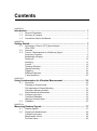
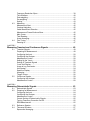


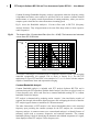


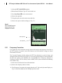
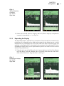

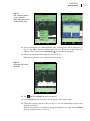
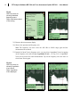

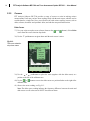
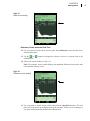

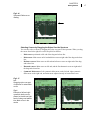
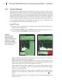
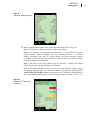

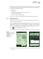
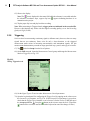


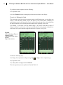


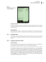
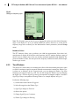


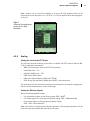
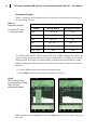


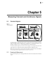
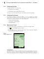
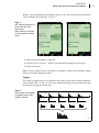
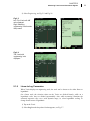


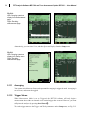
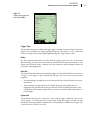
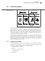
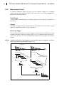


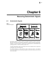


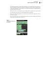


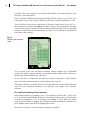

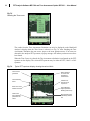


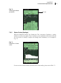
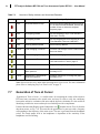
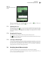


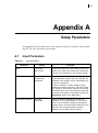

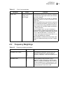
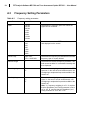

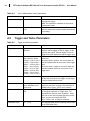


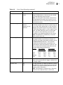
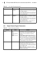


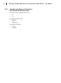


![[Italian]Documentazione Tecnica: Analizzatori portatili](http://vs1.manualzilla.com/store/data/006162879_1-c9f956b7ab0328a00893d3c6418e422c-150x150.png)