Download Using SQUID VSM Superconducting Magnets at Low Fields

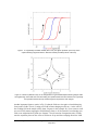
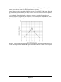
Application Note 1500-011
Using SQUID VSM Superconducting Magnets at Low
Fields
Abstract
The superconducting magnet used in SQUID VSM is capable of generating fields
up to 7 tesla (7x104 gauss) with the value determined to a very high degree of
accuracy over most of this range. The magnetic field value reported to the user is
based only on the current flowing from the magnet power supply. At low fields
(less than 1 tesla), the magnetic field experienced by the user’s sample can
deviate significantly from the reported magnetic field. The magnitude of this
field error as much as 40 gauss in SQUID VSM magnets. The origin of this effect
is described and methods for its mitigation are outlined.
(A similar application note 1070-207 discusses these effects in the context of PPMS magnets)
Section I: Introduction
When using a superconducting solenoid to control the magnetic field in an experiment, the user
must be aware of pinned magnetic flux lines and flux movement within the magnet in order to
better know the magnetic field at the location of the user’s experiment. This application note will
discuss how these effects manifest in the magnet used for the Quantum Design SQUID VSM. As
the title implies, the effects are of greatest relative significance at low fields and are very
important to keep in mind when conducting research on soft magnetic materials whose magnetic
state is strongly affected by small changes in magnetic fields near zero.
Quantum Design does not incorporate a field sensor such as a Hall sensor in its instruments. The
magnetic field reported by the SQUID VSM is based on the current that is being generated in the
magnet power supply (if the magnet is charging), or the last current that was sourced from the
power supply when it was connected to the magnet (if the QuickSwitch on the magnet has been
closed). The magnet power supply current is translated into a magnetic field using a constant
field-to-current conversion factor (or “B/I ratio”) for that given magnet. This yields a magnetic
field value that is very accurate at higher fields (above about 1 tesla).
There are two phenomena that cause the SQUID VSM reported magnetic field to differ from the
actual magnetic field at the location of the user’s sample. Below is a brief summary of these
effects. The remainder of this application note will describe each these phenomena in greater
detail.
1) Magnet remanence: alloys such as those used in the windings of superconducting
magnets will permit the magnet field to enter the superconducting material as threads of
quantized magnetic flux when placed in sufficiently large magnetic fields. These flux
lines are “pinned” and immobilized at defects in the material. Movement of flux lines
Quantum Design
Application Note 1500-011, Rev. A0
May 2010
1
causes energy dissipation and can destroy the superconducting state. When the magnetic
field is removed (for our case, when the magnet current is set back to zero from a high
field), some of these pinned flux lines remain behind and create a small magnetic field
seen at the sample location.
2) Flux creep and escape: over time, some of these pinned magnetic flux lines will
redistribute and may even leave the wire material altogether. The term “flux creep”
describes the diffusion of flux lines inside a superconductor. At a stable magnetic field,
escape of flux from the interior of the wire can lead to induced currents in the magnet due
to the topology of the superconducting magnet.
An outline of this note is as follows: Section II will discuss the first two effects of remanence and
flux motion. Section III presents methods for mitigating the magnetic field artifacts that have
been described.
Before reading this application note, it is important to understand the basics of magnetic field
control in the SQUID VSM, especially the principle of the superconducting QuickSwitch, as
described in section 3.4 of the SQUID VSM User Manual. Familiarity with superconducting
phenomena, especially the mixed state of type II superconductors, is also highly recommended as
this note will not provide that background (see ref. 1)
Section II: magnet remanence and flux motion
The effect of magnet remanence at low fields is an offset error in the reported magnetic field.
This offset is dependent on the magnet history and is opposite in sign when coming from positive
versus negative fields. Figure 1 below illustrates how this offset manifests in DC magnetometer
data for a sample that is magnetically reversible. If one plots the magnetic moment vs. the
reported SQUID VSM magnetic field, the red curve results. Note that the hysteresis curve is
“inverted” so that there is an apparently negative coercivity for the sample! On the other hand, if
one were to plot the moment vs. the actual magnetic field at the sample location, the reversible
blue M(H) curve results. While it is unphysical for the entire M(H) hysteresis loop to be inverted
(it implies continuous heat absorption by the material as one cycles the field) it is possible to have
a locally inverted region of the loop. The existence of locally inverted hysteresis loops is of
interest to the research community, so it is important to discern real sample physics from
instrument artifacts, as pointed out in ref. 2.
If we define the field error as:
field error = (real magnetic field at the sample) – (reported field)
and plot this quantity as a function of the field in a typical SQUID VSM magnet (see Fig. 2), we
see that the absolute error decreases at higher fields, the sign of the field error depends on the
direction of magnet charging, and that switching the field charging direction results in the field
error traversing to the appropriate leg in a short field duration (see traversing lines at -3 and +5
tesla).
2
Application Note 1500-011, Rev. A0
May 2010
Quantum Design
Figure 1. A magnetically reversible material (blue curve) can appear hysteretic (red curve) due to
superconducting magnet remanence. Note the inverted (clockwise) nature of the loop.
Figure 2. Field error (defined in text) vs. the charge field in a typical SVSM superconducting magnet. Note
the negative sign of the field error when decreasing from positive fields. Note also that the error is generally
not symmetric between and up and down legs and is peculiar to each magnet.
Another important feature to notice in Fig. 2 is that the field error is negative when discharging
from positive fields. That is, if setting zero field in linear charging mode from +1 tesla or above,
the resulting field at the sample will be about -20 gauss in this example. So, if one wants to reach
true zero field it means stopping the field discharge short at +20 Oe instead of overshooting zero
field as one might intuitively think (see footnote 3 for a discussion of magnetism units). Finally,
note the asymmetry between the values of field error for up and down ramping directions. It has
Quantum Design
Application Note 1500-011, Rev. A0
May 2010
3
been observed that the field error magnitude near zero field can differ by up to 15 gauss (this is a
property of a particular magnet) for the different charging directions.
Figure 3 shows the typical magnitude of the field error in a 7 tesla SQUID VSM magnet. Note the
log-normal plot style necessitated by the large variation in the field error as a function of applied
field.
As with the other figures, this should not be used to generate a correction for data taken on a
different system as the magnitude of the remanence varies from magnet to magnet. Rather, these
figures should be used for their qualitative information.
Figure 3. Typical magnitude of average field error (averaged between up and down ramp directions) as a
function of the magnet field for a SQUID VSM magnet. Note that the field error can be as much as 15 gauss
different between up and down ramp directions
4
Application Note 1500-011, Rev. A0
May 2010
Quantum Design
Figure 4. The magnetic field at the sample location, as measured using a paramagnetic Dy2O3 sample,
slowly drifts by about 1 gauss upon setting zero field in LINEAR mode from +7 tesla. After 1 hour, the field
was once again set to zero which heats the QuickSwitch and removes persistent currents. See the diagram
on the next page for an explanation of this phenomenon.
The effect of magnetic flux motion on the magnetic field at the sample location is illustrated in
Fig. 4. The field was set from +7 tesla to zero in linear mode and stabilized. The effects shown
here are seen to be independent of the initial field providing it was larger than +1 tesla.
These unusual observations can be explained by the fact that a small amount of pinned remanent
magnetic flux in the magnet escapes from the magnet windings into the bore of the magnet . In
order to understand this, note that when the QuickSwitch is in the superconducting state it will
sustain small DC currents without dissipation. This means that the current in the magnet can
differ slightly from the current at the power supply when the QuickSwitch is in the
superconducting state, a fact which should be kept in mind for the discussion below. As
illustrated in the table and the accompanying figure below, a magnet is originally in its virgin
state (1) in which no flux is pinned inside it. Upon heating (opening) the QuickSwitch and
passing current in the magnet windings (2), a positive field is generated in the sample space at the
center. After removing the current in the magnet and cooling (closing) the QuickSwitch (3), some
flux remains pinned in the magnet and has the same sign as the original field because it resulted
from field lines penetrating the magnet at positive fields.4 However, the stray fields from these
“dipoles” are of course of the opposite sign, hence the negative initial remanent field at the
sample location after discharging from positive fields. After an hour in this state, a small fraction
of the pinned flux lines have escaped from the magnet windings and are in the bore of the magnet
(4). Since this flux is now in free space, it must be represented by currents flowing in the magnet
and these are in the direction of the original magnetic field. Since the magnet is superconducting
(the QuickSwitch acts as a persistent switch at small currents like this), these currents will not
dissipate. The small amount of flux escape has a large effect on the field at the sample location
due to a field amplification effect: the field (seen at the sample location) when the flux has moved
into the bore of the magnet is much larger than the stray field when that same amount of flux was
pinned in the magnet.5 Upon heating the QuickSwitch and setting zero field (5), the power supply
removes the positive current in the magnet and the field that remains at the sample location is due
to the stray fields from the remaining pinned vortices in the magnet. The magnetic field at the
sample is nearly the same as in state (3) because the vast majority of the flux has remained pinned
in the magnet.
Quantum Design
Application Note 1500-011, Rev. A0
May 2010
5
top view of magnet
magnet
switch
state
state
Imagnet
Bsample
1
virgin
closed
0
0
2
charged
open
I2 > 0
B2 > 0
3
remanent
closed
I3 = 0
B3 < 0
closed
I4 > 0
B4 > B3
open
I5 = 0
B5 ≅ B3
Step
4
remanent
+ 1 hour
5
remanent,
reconnected
6
Application Note 1500-011, Rev. A0
May 2010
Quantum Design
Section III: mitigating magnetic field artifacts in measurements
The magnitude of the remanence in the magnet can typically be reduced down to 1-2 gauss by
setting the field to zero (from an initial field above 1 tesla) in oscillate mode. This will also
attentuate the flux creep effects. Remanence can be further reduced down to <0.05 gauss by using
the Ultra Low Field option for the SQUID VSM which employs a fluxgate magnetometer and the
modulation coil in the magnet to compensate trapped flux from the magnet.
Once a low-remanence state has been achieved in the magnet, you can make measurements at low
fields (-100 Oe < H < +100 Oe) without inducing a significant amount of remanence. However, a
field of 1 kOe will already introduce a lot of pinned flux in the magnet.
Some measurement situations (most commonly M(H) loops from high fields through zero field)
do not permit the use of low field techniques discussed above. In this case there are some
guidelines we recommend in order to achieve best results:
•
Determine the magnet remanence and flux creep properties of your magnet
(see Figs. 2 - 5) by using a pure paramagnetic sample such as the Er:YAG standard
sample (4500-636) or a Dy2O3 pellet (4041-008) that is free of any measureable amount
of ferromagnetic impurities (very important – a ferromagnetic signature will lead to an
underestimate of the real magnet remanence value); this option is good since in principle
the M(H) slope for these materials is very nearly constant at 300 K so one can determine
the absolute field error at each field – contact [email protected] for more information.
•
The remanence properties of the magnet are very reproducible as long as the same field
charging recipe is followed each time; thus, once the field error table is determined by
using a standard sample, you can run the same field charging sequence on your sample
and apply this field correction; alternately, you can modify the field set points of the
measurement protocol so that the actual field is the desired one (in the example from Fig.
2, setting +20 Oe from positive high fields will produce a field at the sample of ~0 Oe).
In conclusion, one must be cautious when using a magnet used for generating ~104 gauss to also
accurately generate fields on the order of 10 gauss. By understanding the basic operating
principles of a superconducting magnet and by following the guidelines laid out above, it is
possible to greatly reduce artifacts in the reported magnetic field.
While we have focused here on the instance of the Quantum Design SQUID VSM, the effects of
remanence, flux creep and persistent switch leakage currents discussed in this application note are
relevant to any superconducting magnet with a superconducting switch.
Quantum Design
Application Note 1500-011, Rev. A0
May 2010
7
1
M. Tinkham, Introduction to Superconductivity (McGraw-Hill, 1996).
2
“Soft-magnetic materials characterized using a superconducting solenoid as magnetic source” Giovanni
Mastrogiacomo, Jorg F. Löffler, and Neil R. Dilley, Appl. Phys. Lett. 92, 082501 (2008),
DOI:10.1063/1.2838733
3
Note on the magnetic units convention: we refer here to the magnetic field B in units of gauss (where 104
gauss = 1 tesla) and it represents the real magnetic field at the sample. In contrast, the magnetic induction H
is expressed in oersted (Oe) and, being defined as the field due to free currents, this is the one that the user
controls when setting a current at the magnet power supply. In SI units, B = m0(H + M) where M is the
magnetization density and is defined as arising from bound currents. For more information, see the
Magnetic Units Conversion Table under Technical Resources at the Quantum Design website
www.qdusa.com .
4
For viewing clarity in the figure, the magnetic field lines in the superconductor do not show the
supercurrent vortices that generate the magnetic field.
5
Consider the persistent magnet as a superconducting ring of inner dimension of R and the pinned flux line
in the superconductor with a radius r, where R >> r. Referring to the states in Table 1, we must compare
the magnetic field at the sample location (taken as the origin) between the initial remanent state (3) and
when the vortex moves out of the ring into the middle (4).
We know that flux is conserved:
Φ = B3 (R ) ⋅ r 2 = B4 (0 ) ⋅ R 2
That is, the flux enclosed on vortex at position R (at the inner bore of the magnet) is compared with field in
the bore of the magnet after the vortex moves out.
The equation above approximates the magnetic field B as constant over the area of the loops in both cases.
While this is not strictly true, the error is small compared with the amplification effect we are observing
and hence is neglected.
magnetic moment of vortex: m = π r ⋅ I
where I is the current flowing around perimeter.
2
magnetic field at center of the vortex (a current ring): B3 (R ) =
put this value of I into above expression for moment:
m=
2π
μ0 ⋅ I
2r
B3 (R )r 3
μ0
magnetic field at sample location due to pinned flux “dipole”: B3 (0 ) = −
B (R ) ⎛ r ⎞
insert expression for m from above: B3 (0 ) = − 3
⋅⎜ ⎟
2
⎝R⎠
μ0 m
⋅
4π r 3
3
Use flux conservation equation to compute ratio of field seen at sample in state 4 vs. state 3:
B4 (0)
R
= −2
B3 (0 )
r
Since R~2.5cm and r ~10-3 cm, this amplification is over x1000.
This is why a tiny amount of flux creep out of magnet will have a large effect on the field seen at the
sample location.
8
Application Note 1500-011, Rev. A0
May 2010
Quantum Design