Download MScMS (Mobile Spatial coordinate Measuring System)

Politecnico di Torino
Porto Institutional Repository
[Doctoral thesis] Design and development of a new large-scale metrology
system: MScMS (Mobile Spatial coordinate Measuring System)
Original Citation:
Maisano Domenico (2008). Design and development of a new large-scale metrology system:
MScMS (Mobile Spatial coordinate Measuring System). PhD thesis
Availability:
This version is available at : http://porto.polito.it/2544537/ since: May 2014
Published version:
DOI:10.6092/polito/porto/2544537
Terms of use:
This article is made available under terms and conditions applicable to Open Access Policy Article
("Public - All rights reserved") , as described at http://porto.polito.it/terms_and_conditions.
html
Porto, the institutional repository of the Politecnico di Torino, is provided by the University Library
and the IT-Services. The aim is to enable open access to all the world. Please share with us how
this access benefits you. Your story matters.
(Article begins on next page)
POLITECNICO DI TORINO
DOCTORATE IN PRODUCTION SYSTEMS & INDUSTRIAL
DESIGN
♦
DESIGN AND DEVELOPMENT OF A NEW LARGE-SCALE
METROLOGY SYSTEM: MSCMS (MOBILE SPATIAL
COORDINATE MEASURING SYSTEM)
Supervisor:
Ph. D. Student:
Prof. F. Franceschini
Domenico MAISANO
May 2008
Executive summary
This thesis arises from the research activity developed at the Industrial Metrology and
Quality Engineering Laboratory of DISPEA – Politecnico di Torino, on a new system
prototype for dimensional measurement, called Mobile Spatial coordinate Measuring System (MScMS) [Franceschini et al., 2008-II]. MScMS determines dimensional features of
large-size objects and has been designed to overcome some limits shown by other widespread measuring sets used nowadays, like Coordinate Measuring Machines (CMMs),
theodolites/tacheometers, photogrammetry equipments, GPS based systems, Laser Trackers [Bosch, 1995; Pozzi, 2002].
Basing on a distributed sensor networks structure, MScMS can accomplish rapid dimensional measurements, in a wide range of indoor operating environments. It consists of
distributed wireless devices, communicating with each other through radiofrequency (RF)
and ultrasound (US) transceivers. This frame makes the system easy to handle and to
move, and gives the possibility of placing its components freely around the workpiece.
The wireless devices − known as “Crickets” − are developed by the Massachusetts Institute of Technology (MIT). Being quite small, light and potentially cheap (if mass produced), they fit to obtain a wide range of different network configurations [Priyantha et
al., 2000; Balakrishnan et al., 2003].
These features make the new system suitable for particular types of measurement,
which can not be carried out, for example, by conventional CMMs. Typical is the case of
large-size objects which are unable to be transferred to the measuring system area (because of their dimensions or other logistical constraints) and thus require the measuring
system to be moved to them.
In the dissertation the system is described exhaustively and characterized through practical experiments. Then, the system is compared to classical CMMs and the indoor-GPS
(iGPS), an innovative laser based system for large-scale metrology. Finally, future directions of this research are given.
Contents
List of acronyms and abbreviations .............................................................................. vii
1. Introduction.................................................................................................................. 1
1.1 The Mobile Spatial coordinate Measuring System (MScMS) ............................... 1
1.2 The new paradigm of the distributed measuring systems ...................................... 1
1.3 Literature review .................................................................................................... 1
1.4 Organization of the dissertation ............................................................................. 1
2. Principle functioning and MScMS architecture ....................................................... 1
2.1 Introduction............................................................................................................ 1
2.2 System requirements and comparison with other measuring techniques............... 1
2.3 MScMS hardware equipment................................................................................. 1
2.3.1 Cricket devices............................................................................................ 1
2.3.2 Evaluation of distances between Cricket devices ....................................... 1
2.3.3 Crickets communication ............................................................................. 1
2.3.4 The mobile probe ........................................................................................ 1
2.4 MScMS software architecture................................................................................ 1
2.4.1 Location of Crickets mounted on the mobile probe.................................... 1
2.4.2 Location of points touched by the probe tip................................................ 1
2.4.3 Cricket firmware ......................................................................................... 1
2.4.4 Semi-automatic location of the constellation.............................................. 1
3. MScMS prototype ........................................................................................................ 1
3.1 Introduction............................................................................................................ 1
3.2 Description of the first MScMS prototype............................................................. 1
3.3 MScMS actual performance, critical aspects and possible improvements............. 1
3.4 Final considerations ............................................................................................... 1
4. Experimental evaluation of the MScMS ultrasound transducers ........................... 1
4.1 Introduction............................................................................................................ 1
4.2 Piezo-electric US transducers ................................................................................ 1
4.3 Factors affecting US transceivers........................................................................... 1
4.4 Analysis of the experimental results ...................................................................... 1
4.4.1 Results of the factorial plan ........................................................................ 1
4.4.2 Interpretation of the results ......................................................................... 1
4.4.3 Additional experiments ............................................................................... 1
4.5 Final notes and future work.................................................................................... 1
5. MScMS and CMMs: a structured comparison ......................................................... 1
5.1 Introduction............................................................................................................ 1
5.2 CMMs main characteristics.................................................................................... 1
5.3 Comparison criteria................................................................................................ 1
5.3.1 Portability.................................................................................................... 1
vi
Contents
5.3.2 Working volume.......................................................................................... 1
5.3.3 Set up........................................................................................................... 1
5.3.4 Metrological performances ......................................................................... 1
5.3.5 Measurements system diagnostics............................................................... 1
5.3.6 Ease of use................................................................................................... 1
5.3.7 Flexibility .................................................................................................... 1
5.3.8 Cost ............................................................................................................. 1
5.3.9 System management.................................................................................... 1
5.4 Final considerations................................................................................................ 1
6. iGPS performance evaluation and comparison with MScMS ................................. 1
6.1 Introduction ............................................................................................................ 1
6.2 iGPS structure ........................................................................................................ 1
6.3 iGPS technology and operating features ................................................................ 1
6.4 Factors affecting measurement............................................................................... 1
6.5 Experimental work for iGPS’ preliminary performance analysis .......................... 1
6.6 Systems comparison ............................................................................................... 1
6.7 Summary and final considerations ......................................................................... 1
7. Future wireless sensor networks................................................................................. 1
7.1 Introduction ............................................................................................................ 1
7.2 Typical features of sensor networks ....................................................................... 1
7.3 Growth potential and future advancement ............................................................. 1
7.4 Final considerations................................................................................................ 1
8. Conclusions and future directions .............................................................................. 1
References .......................................................................................................................... 1
List of acronyms and abbreviations
2D
two-dimensional
3D
three-dimensional
CCD
Charge Coupled Device
CMM
Coordinate Measuring Machine
CNC
Computer Numerical Control
CSAIL
Computer Science and Artificial Intelligence Lab
DISPEA
Dipartimento di Sistemi di Produzione ed Economia dell’Azienda
DoE
Design of Experiments
EF
Error Function
GPS
Global Position System
GUM
Guide to the expression of Uncertainty in Measurement
ICT
Information and Communications Technology
IEC
International Electrotechnical Commission
IEEE
Institute of Electrical and Electronics Engineers
iGPS
indoor GPS
IP
Internet Protocol
LED
Light Emitting Diode
MIT
Massachusetts Institute of Technology
MPE
Maximum Permitted Error
MScMS
Mobile Spatial coordinate Measuring System
PC
Personal Computer
PVDF
Polyvinylidene fluoride
RF
Radio Frequency
RH
Relative Humidity
T
Temperature
TDoA
Time Difference of Arrival
TOF
Time of flight
US
Ultrasound
V-bar
Vector bar
VIM
International Vocabulary of Basic and General Terms in Metrology
WSN
Wireless Sensor Network
1.
Introduction
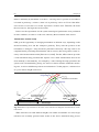
The field of large-scale metrology can be defined as the metrology of large machines and
structures that is to say “the metrology of objects in which the linear dimensions range
from tens to hundreds of meters” [Puttock, 1978]. There is an increasing trend for accurate measurement of length, in particular, the 3D coordinate metrology at length scales of
5m to 100m has become a routine requirement in industries such as aircraft and ship construction. In this direction, there have been significant advances across a broad range of
technologies, including laser interferometry, absolute distance metrology, very high density CCD (Charge-Coupled Device) cameras and so on.
Many types of metrological equipments, utilizing different kind of technologies (optical, mechanical, electromagnetic etc..), give physical representations of measured objects
in a three-dimensional Cartesian coordinate system. Coordinate Measuring Machines
(CMMs), theodolites/tacheometers, photogrammetry equipments, GPS (Global Positioning Systems), Laser Trackers are typical instruments to do it. Each of these systems is
more or less adequate, depending on measuring conditions, user’s experience and skill,
and other factors like time, cost, size, accuracy, portability etc.. Classical CMMs, that
make possible performing repeated and accurate measurements on objects which are even
complexly shaped, are widespread. On the other hand, CMMs are generally bulky and not
always suitable for measuring large size objects (for example, longerons of railway vehicles, airplane wings, fuselages etc..), because the working volume is limited [ISO 10360,
part 2, 2001]. In general, for measuring medium-large size objects, portable systems can
be preferred to fixed ones. Transferring the measuring system to the measured object
place is often more practical than the vice-versa [Bosch, 1995]. Systems as
theodolites/tacheometers, photogrammetry equipments, Laser Trackers, or GPS − rather
than CMMs − can be easily installed and moved [Pozzi, 2002]. However, they can have
some other drawbacks as mentioned in the remaining of this thesis (Section 2.2).
2
Chapter 1
1.1
The Mobile Spatial coordinate Measuring System (MScMS)
This thesis introduces a new measuring system called Mobile Spatial coordinate Measuring System (MScMS), developed at the Industrial Metrology and Quality Laboratory of
DISPEA – Politecnico di Torino. MScMS has been designed to perform simple and rapid
indoor dimensional measurements of large-size objects (large scale metrology). An essential requirement for the system is portability − that is the aptitude to be easily transferred
and installed.
MScMS is made up of three basic parts: (1) a “constellation” of wireless devices
(Crickets), (2) a mobile probe, and (3) a PC to store and elaborate data [MIT C.S.A.I.L.,
2004]. Crickets and mobile probe exploit ultrasound (US) transceivers in order to evaluate mutual distances. The constellation devices act as reference points, essential for the
location of the probe.
Each US device has a communication range limited by a cone of transmission within
an opening angle of about 170° and a maximum distance of no more than 8 m. The mobile probe location in the working volume is obtained by a trilateration. Consequently, the
probe can be located only if it communicates with at least 4 constellation devices at once
[Akcan et al., 2006].
The system makes it possible to calculate the position – in terms of spatial coordinates
– of the object points “touched” by the probe. Acquired data are then available for different types of elaboration to determine the geometric features of the measured objects (distances, curves or surfaces).
One of the most critical aspects in the system set-up is the constellation devices positioning. Constellation devices operate as reference points, or beacons, for the mobile
probe. In principle, Crickets can be positioned without restriction all around the measured
object. However, the number and position of constellation devices are strongly related to
the dimensions and shape both of the measuring volume and the measured object. It is
important to assure a full coverage of the space served by constellation devices by a
proper alignment of US transmitters. The spatial location of the constellation devices follows a semi-automatic procedure. The accuracy in the location of constellation devices is
fundamental for the accuracy in the next mobile probe location [Patwary et al., 2005].
Introduction
3
1.2 The new paradigm of the distributed measuring systems
For the purpose of discussion, the large-scale dimensional measurement systems can be
classified into centralized and distributed systems. In the case of centralized instruments,
measurements may independently arise by a single stand-alone unit which is a centralized
complete system (i.e. a CMM, a laser-scanner or a Laser Tracker), while distributed instruments are made of two or more distributed units (i.e. MScMS or other innovative systems like the indoor-GPS, described in Chap. 6 [Metris, 2007]).
Distributed measurement systems introduce a new paradigm in the field of large-scale
metrology. Due to their nature, they are portable and can be easily transferred around the
area where the measurand is. Compared to centralized systems, distributed systems may
cover larger measuring areas, with no need for repositioning the instrumentation devices
around the measured object [Kang et Tesar, 2004].
MScMS can be classified as a modular distributed measuring system for large volume
objects. Even if at present time MScMS is still a prototype and needs to be further developed, the system enables factory-wide location of multiple objects, applicable in manufacturing and assembly. Mainly, it can be used by aerospace manufacturers, but can also
be adopted by automotive and industrial manufacturers both for positioning and tracking
applications. Since MScMS main components are a number of wireless devices distributed around the measuring area, this not rigidly connected frame makes the system easy
to handle and to move, and gives the possibility of placing its components freely around
the workpiece, adapting to the environment and not requiring particular facilities. As a
consequence, MScMS is suitable for particular types of measurement, which can not be
carried out by traditional frame instruments, like conventional CMMs, because they are
bulky and cannot be comfortably moved.
The introduction of distributed measuring systems will probably have important effects
on simplifying the current measuring practices within large scale industrial metrology
[Maisano et al., 2007]. This tendency is confirmed by other recent distributed measuring
systems based on laser and optical technology: the indoor-GPS (iGPS), the PortableCMM and the Hi-Ball [ARC Second, 2004; Metris, 2007; Metronor, 2007; Welch et al.,
2001]. All these systems – even they use different technologies – are composed of a
number of sensors, arranged around the measuring area, which can be viewed by a sensor
probe measuring the object surface.
4
Chapter 1
1.3 Literature review
Dramatic advances in integrated circuits and radio technologies have made the use of distributed wireless sensor networks (WSNs) possible for many applications [Neil, 2005].
Recently, the attention towards the utilization of systems based on distributed sensor devices in manufacturing is increasing. Since sensor devices do not need cables and may be
easily deployed or moved, they can be practically utilized for a variety of industrial applications – factory logistics and warehousing, environmental control and monitoring, support for assembly processes, industrial dimensional measuring and real-time surveillance
are only some possible applications. While outdoor localization applications are widespread today (e.g. Global Positioning System – GPS), indoor applications can also benefit
from location determination knowledge [Gotsman and Koren, 2004]. To make such applications feasible, the device costs should be low and the network should be organized
without significant human involvement.
To give a concrete idea of the potential of the systems based on WSNs in manufacturing, here are briefly introduced some of the most interesting research issues with the corresponding bibliographic references.
Support for final assembly. Ultrasonic sensors are mounted on power tools – for example
screwdrivers – to detect their real position and activate them if they are in the right position, during final assembly [Pepperl+Fuchs, 2005].
Industrial control and monitoring. Sensor devices can be deployed to perform industrial
control and monitoring (for instance control of the air conditions of pollution, temperature, and pressure in different areas of the factory) or for emergency responses in case of
incidents [Doss and Chandra, 2005; Pan et al., 2006; Koumpis et al., 2005; Oh et al.,
2006].
Factory logistics and warehousing. In an industrial warehouse mobile forklifts generally
move along corridors in order to reach the shelves where goods are stored. Forklifts and
shelves can be equipped with ultrasound transceivers that communicate with each other,
with the purpose of evaluating mutual distances [Intel Corporation, 2005]. This type of
wireless sensor network can be utilized to calculate the position of the forklifts for:
• Indoor Navigation. Mobile forklifts, equipped with wireless transceiver, are automatically guided towards their destination [Wang and Xi, 2006];
Introduction
5
• Traffic Monitoring. The physical traffic can be monitored in order to identify the most
congested areas or to improve goods distribution [Capkun et al., 2001].
Large-scale dimensional measuring. Besides the MScMS, two innovative measuring systems for large scale dimensional measurements are the 3rd Tech Hi-Ball and Metris iGPS
[Welch et al., 2001; Rooks, 2004; Metris, 2007]. These systems − all based on optical
technologies and recently industrialised − are lightweight and very accurate, but they are
relatively high priced and generally require a relatively large time for installation and
start-up. Recently, the iGPS performance was studied and tested during a three months
research activity carried out at the University of Bath (UK), attending the project LVMA
(Large Volume Metrology Assembly − http://www.bath.ac.uk). A detailed description of
this system and a comparison with MScMS is presented in Chap. 6.
1.4 Organization of the dissertation
The remainder of this dissertation contains a detailed description of the principle functioning and the implementation of MScMS. Then, the system performance is evaluated
and compared with two other existing systems for large-scale dimensional measurements:
the CMMs and the iGPS. More specifically, the thesis is structured like this:
• Chap. 2 presents the MScMS design features and modus operandi. In particular, the attention is focused on the system principle functioning and the hardware/software architecture.
• Chap. 3 describes the first MScMS prototype, presenting a preliminary experimental
evaluation of its metrological performance. Also, this chapter identifies the system
critical aspects and possible improvements.
• Chap. 4 concentrates the attention on the main features of the US transceivers equipping the system. They are deeply analysed by means of a structured experimental plan.
• Chap. 5 provides a structured comparison between MScMS and the classical CMMs.
• Chap. 6, discusses the iGPS technological features and principle, and provides a comparison with the MScMS.
• Chap. 7 presents a short general analysis of the development of WSNs. This can be interesting, considering that MScMS and other innovative measuring systems are based
on distributed WSNs.
6
Chapter 1
• Finally, Chap. 8 summarizes the thesis contributions and mentions possible future directions for improving the MScMS performance.
2.
Principle functioning and MScMS architecture
2.1 Introduction
The purpose of this chapter is to describe the MScMS hardware/software/firmware architecture and functionalities.
Before introducing MScMS, in Section 2.2 we provide a structured description of requirements and functionalities that a generic system for large-scale dimensional measurements should meet. At the same time, we present a taxonomy of the most common
techniques and metrological equipments for dimensional measuring. Major advantages
and drawbacks are highlighted. The attention is subsequently focused on the MScMS design, analysing in detail the following aspects: hardware and software configuration, discussion of the location algorithms implemented by MScMS, description of the semiautomatic procedure for the spatial location of the MScMS constellation devices.
2.2 System requirements and comparison with other measuring
techniques
MScMS has been designed to perform dimensional measurements of medium-large size
objects – with dimensions up to 30÷60 meters. It should be easy to move and install, lowpriced and able to work indoor (inside warehouses, workshops, laboratories).
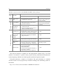
Tab. 2.1 identifies the MScMS basic requirements.
Considering them, we briefly analyse the most common measuring tools and techniques. Tab. 2.2 shows the result of a qualitative comparison among five measuring instruments: theodolite/tacheometer, CMM, Laser Tracker, photogrammetry system, and
GPS. The last row of the table takes account of MScMS target performances.
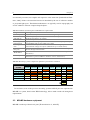
Different considerations rise from Tab. 2.2. CMMs − in spite of being very accurate
measuring instruments − are expensive, bulky and not easily movable. On the other hand,
theodolites or GPS are smaller and lightweighter but not very flexible, in terms of different types of measurements offered. Even more, GPS systems are less accurate, and cannot
operate indoor. Interferometrical Laser Trackers and digital photogrammetry equipments
8
Chapter 2
are extremely accurate, but complex and expensive at the same time [Sandwith and Predmore, 2001]. Points to be measured need to be identified by the use of reflective markers
or projected light spots. Theodolites/tacheometers are typically used in topography, but
are not suitable to measure complex shaped objects.
Tab. 2.1 Definition and description of MScMS basic requirements
Requirement
Description
Portability
Fast Installation
and Start-Up
Low Price
Metrological
Performances
Working Volume
Easy to move, easy to assemble/disassemble, lightweight and small sized.
Before being ready to work, system installation, start-up or calibration
should be fast and easy to perform.
Low costs of production, installation and maintenance.
Appropriate metrological performances, in terms of stability, repeatability,
reproducibility and accuracy [ISO 5725, 1986].
The area covered by the instrument, should be wide enough to perform
measurements of large size objects (dimensions up to 30÷60 meters).
System should be user-friendly. An intuitive software interface should guide
the user through measurements.
System should be able to work indoor (inside warehouses, workshops, or
laboratories).
System should be able to perform different measurement typologies (i.e. determination of point coordinates, distances, curves, surfaces etc..).
Easy Use
Work Indoor
Flexibility
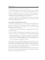
Tab. 2.2. Measuring systems comparison: qualitative performance evaluation
MEASURING
SYSTEM
REQUIREMENTS
Installation
Portability
and Start-Up
Cost
Metrological
Performances
Working
Volume
Easy Use
Work
Indoor
Flexibility
THEODOLITE
HIGH
FAST
LOW
LOW
LARGE
MEDIUM
YES
LOW
CMM
LOW
SLOW
HIGH
HIGH
SMALL
HIGH
YES
HIGH
LASER TRACKER
MEDIUM
MEDIUM
MEDIUM
HIGH
LARGE
LOW
YES
MEDIUM
PHOTOGRAMMETRY
MEDIUM
SLOW
MEDIUM
MEDIUM
MEDIUM
LOW
YES
MEDIUM
GPS
HIGH
FAST
MEDIUM
LOW
LARGE
HIGH
NO
LOW
MScMS (Purpose)
HIGH
MEDIUM
LOW
MEDIUM
LARGE
HIGH
YES
HIGH
☺
Key
In conclusion, none of the previous measuring systems fulfil all previous requirements.
MScMS is a system, based on the WSN technology, able to make a trade-off among these
requirements.
2.3 MScMS hardware equipment
MScMS is made up of three basic parts [Franceschini et al., 2008-II]:
Principle functioning and MScMS architecture
9
1. a “constellation” of wireless devices, distributed around the measuring area;
2. a mobile probe to register the coordinates of the object “touched” points;
3. a PC to store data sent – via Bluetooth – by the mobile probe and an ad hoc application
software.
The mobile probe is equipped with two wireless devices, identical to those making up
the constellation. These devices, known as Crickets, are developed by Massachusetts Institute of Technology and Crossbow Technology. They utilize two US transceivers in order to communicate and evaluate mutual distances [MIT C.S.A.I.L., 2004; Crossbow
Technology, 2008]
The system makes it possible to calculate the position – in terms of spatial coordinates
– of the object points “touched” by the probe. More precisely, when a trigger mounted on
the mobile probe is pulled, the current coordinates of the probe tip are calculated and sent
to a PC via Bluetooth. Acquired data are then available for different types of elaboration
(determination of distances, curves or surfaces of measured objects).
Constellation devices (Crickets) operate as reference points, or beacons, for the mobile
probe. The spatial location of the constellation devices follows a semi-automatic procedure, described in Subsection 2.4.4. Constellation devices are distributed without constraint around the object to measure. In the following subsections, we describe the
MScMS hardware, focusing on:
• the wireless (Crickets) devices (Subsection 2.3.1);
• the measuring method to evaluate mutual distances among Crickets (Subsection 2.3.2);
• the mobile probe (Subsection 2.3.3).
2.3.1 Cricket devices
Cricket devices are equipped with radiofrequency (RF) and ultrasound (US) transceivers.
Working frequencies are respectively 433 MHz (on RF) and 40 kHz (on US). Cricket devices are developed by Massachusetts Institute of Technology and manufactured by
Crossbow Technology. Each device uses an Atmega 128L microcontroller operating at
7.4 Mhz, with 8 kBytes of RAM, 128 kBytes of FLASH ROM (program memory), and 4
kBytes of EEPROM (as mostly read-only memory). Alimentation is provided by two
“AA” batteries of 1.5 V [Balakrishnan et al., 2003].
10
Chapter 2
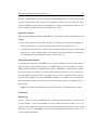
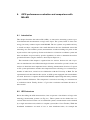
Cricket devices are quite small (see Fig. 2.1) easy to be moved, and cheap (each unit
would cost about 10÷20 €, if mass-produced). Due to these characteristics, they are
optimal for ad hoc WSN applications [Priyantha et al., 2000].
Ultrasound Transmitter
(c)
a
Integrated antenna for
RF transceiving
≈1.2 cm
≈ 9 cm
b
c
(a)
(b)
Ultrasound Receiver
≈ 4 cm
photo
perspective view
orthogonal projection
Fig. 2.1. Cricket Device (Crossbow Technology)
The US transceivers equipping Crickets are quartz crystals, which transform electric
energy in acoustic, and vice-versa (piezo-electric effect). They generate/receive 40 kHz
ultrasound waves. Transmitters, excited by electric impulses, vibrate at the resonance frequency producing acoustic ultrasound impulses [ANSI/IEEE Std. 176-1987, 1988]. On
the other hand, receivers transform the vibration produced by ultrasonic waves in electric
impulses. A detailed characterization of these transducers is presented in Chap. 4.
2.3.2 Evaluation of distances between Cricket devices
Crickets devices continuously communicate each other in order to evaluate mutual distances. Devices communication range is typically 6-8 meters, in absence of interposed
obstacles.
The technique, implemented by each pair of Crickets to estimate mutual distance, is
known as Time Difference of Arrival (TDoA). It is based on the comparison between the
propagation time of two signals with different speed (RF and US in this case) [Savvides
et al., 2001]. TDoA technique is described as follows:
a) At random time intervals, included between 150 and 350 milliseconds, each device
transmits a RF query-packet to other devices within its communication range, checking
Principle functioning and MScMS architecture
11
if neighbouring Crickets are ready to receive a US signal (Fig. 2.2-a) [Priyantha et al.,
2000];
b) Ready devices reply sending a RF acknowledgement authorizing next signals transmission (Fig. 2.2-b);
c) Querying Cricket is now authorized to concurrently send a RF and US signal (Fig. 2.2c);
transmitting device
(a) Query (RF)
receiving device
RF
Antenna for RF transmission
(b) Reply (RF) and authorization
for signals transmission
RF
US
(c) Concurrent transmission of RF
and US signals
RF
US transmitter
US receiver
Fig. 2.2. Communication scheme implemented by Cricket devices [Priyantha et al., 2000]
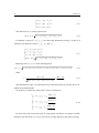
d) The receiving devices measure the time lapse between reception of RF and US signals
(see Fig. 2.3).
transmitting device
receiving device
RF (c - speed of electromagnetic radiation)
query (RF signal)
concurrent transmission
of RF and US signals
RF
RF authorization for
next transmission
RF
US (s - speed of sound)
Δt (TDoA)
time lapse between
reception of RF
and US signals
t
d
Fig. 2.3. Time evolution of RF and US signals: qualitative scheme
t
12
Chapter 2
The distance between two devices is calculated by the following formula:
d=
Δt
1 1
−
s c
(2.1)
where c is the speed of electromagnetic radiations, s the speed of sound, and Δt is
TDoA [Gustafsson and Gunnarsson, 2003].
Due to the large difference between c (about 300,000 km/s) and s (about 340 m/s in air,
with temperature T=20°C and relative humidity RH = 50%):
d ≈ s · Δt
(2.2)
2.3.3 Crickets communication
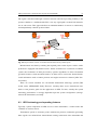
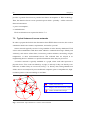
Cricket devices build a wireless network of cooperating sensor nodes. To preserve network scalability, that is to make sure that the amount of information stored by each node
is independent from network dimension (in terms of nodes), each node memorizes the
distances from its direct neighbours contained in the communication range (see Fig. 2.4).
D B2, B4
B2
D B1, B2
B4
D B2, B3
B3
B6
B5
D B4, B8
D B2, B7
D B5, B6
D B4, B9
D B3, B4
D B1, B3
B1
D B4, B5
D B5, B9
D B6, B9
D B3, B8
D B5, B8
D B3, B7
D B1, B7
D B8, B9
D B7, B8
B9
B8
B7
+
B8 communication range
distances received by device B8
distances discarded by B8
distances stored by B8 (and sent to its neighbours)
Fig. 2.4. Distance information handled by a single device (B8) . The shadow highlights the B8
communication range
Principle functioning and MScMS architecture
13
2.3.4 The mobile probe
The mobile probe is equipped with two Cricket devices aligned with the tip and has a
Bluetooth transmitter for sending data to the PC (see Fig. 2.5).
perspective view
orthogonal view
AB
BV
B
V
A
A
B
V
C
G
A, B
C
V
AB, BV
G
Cricket devices
Bluetooth adapter to PC
probe tip (touching measured object)
fixed distances
trigger
C
Fig. 2.5. Schematic representation of the mobile probe
The probe’s Crickets locate themselves using the distance information from the constellation Crickets. The principle is described in Subsection 2.4.1.
System has been designed to be deployed over small or wide areas, depending on the
dimension of the measured objects. The measuring area can be “covered” varying the
number of constellation Crickets.
2.4 MScMS software architecture
This section describes software/firmware features of MScMS for implementing the following operations:
• location of Crickets mounted on the mobile probe;
• location of points touched by the probe;
• communication and data sharing among Cricket devices;
• semi-automatic location of constellation devices.
Fig 2.6 represents the first three operations. All operations are better described in the
following subsections.
14
Chapter 2
(x4, y4, z4)
(x2, y2, z2)
(x3, y3, z3)
distances from device B
distances from device A
(V) point touched by the probe
(x1, y1, z1)
(x5, y5, z5)
PC
V
measured
object
i
d
B
A
(xB, yB, zB)
Operation 2
(xV, yV, zV)
Z
(xA, yA, zA)
Operation 1
X
Y
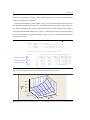
Fig. 2.6. Location of points touched by the probe
2.4.1 Location of Crickets mounted on the mobile probe
Spatial location of each Cricket probe is performed using a trilateration technique. Trilateration uses the known locations of beacon reference points. To uniquely determine the
relative location of a point on a 3D space, at least 4 reference points are generally needed
[Chen et al., 2003; Sandwith and Predmore, 2001; Akcan et al., 2006].
In general, a trilateration problem can be formulated as follows. Given a set of n nodes
(constellation devices) with known coordinates (xi, yi, zi, being i=1÷n) and a set of measured distances Mi, a system of equations can be solved to calculate the unknown position
of a generic point P (u, v, w) (see Fig. 2.7).
⎡ (x1 -u) 2 +(y1 -v) 2 +(z1 -w) 2 ⎤ ⎡ M12 ⎤
⎢
2
2
2 ⎥ ⎢
2⎥
⎢ (x 2 -u) +(y 2 -v) +(z 2 -w) ⎥ = ⎢ M 2 ⎥
⎢
⎥ ⎢# ⎥
#
⎢
⎥ ⎢
⎥
2
2
2
2
⎣⎢ (x n -u) +(y n -v) +(z n -w) ⎦⎥ ⎣⎢ M n ⎦⎥
(2.3)
If the trilateration problem is over defined (4 or more reference points), it can be solved
using a least-mean squares approach [Savvides et al., 2001; Martin et al., 2002].
Each unknown node (generically P) estimates its position by performing the iterative
minimization of an Error Function (EF), defined as:
Principle functioning and MScMS architecture
∑
EF=
n
i=1
15
[M i -G i ]2
(2.4)
n
being:
Mi measured distance between the i-th node and the unknown device (P);
Gi calculated distance between the estimated position of P ≡ (u, v, w) and the known
position of the i-th device Ci ≡ (xi, yi, zi);
n
number of constellation devices (Ci, i=1÷n) within device (P) communication
range.
C2
(x2, y2, z2)
C4
(x4, y4, z4)
M2
C6
(x6, y6, z6)
M6
C8
(x8, y8, z8)
M4
C3
(x3, y3, z3)
M3
M1
M5
C5
(x5, y5, z5)
C7
(x7, y7, z7)
P
(u, v, w)
Z
X
C1
(x1, y1, z1)
P communication range
Y
distances utilized for the location of a device P
C1÷C6
devices within device P communication range
Fig. 2.7. Location of a generic device P
Each of the two Cricket mounted on the mobile probe locates its own position using
the known locations of at least four constellation Crickets, and the measured distance
from them. All information needed for the location is sent to a PC, for a centralized computing.
2.4.2 Location of points touched by the probe tip
The probe tip (V) lies on the same line of devices A and B (see Fig. 2.5). This line can be
univocally determined knowing coordinates of points A ≡ (xA, yA, zA) and B ≡ (xB, yB,
zB), and their distance d(A−V).
The parametric equation of this line is:
16
Chapter 2
⎧x = x A + ( x B − x A ) ⋅ t
⎪
⎨ y = yA + ( yB − yA ) ⋅ t
⎪
⎩z = z A + ( z B − z A ) ⋅ t
(2.5)
The distance d(A−V) can be expressed as:
d(A − V) =
( xA − xv )
2
+ ( yA − yv ) + ( zA − z v )
2
2
(2.6)
Coordinates of point V ≡ (xv, yv, zv) are univocally determined solving a system of 4
equations in 4 unknown values ( x v , y v , z v , and t v ):
⎧x V = x A + ( x B − x A ) ⋅ t V
⎪
⎪⎪ y V = y A + ( y B − y A ) ⋅ t V
⎨z = z + ( z − z ) ⋅ t
A
B
A
V
⎪ V
⎪
2
2
2
⎪⎩d ( A − V ) = ( x A − x v ) + ( y A − y v ) + ( z A − z v )
(2.7)
Replacing terms xV, yV, zV in the fourth equation:
d ( A − V ) = ⎣⎡ x A − x A + ( x B − x A ) ⋅ t V ⎦⎤ + ⎣⎡ y A − y A + ( y B − y A ) ⋅ t V ⎦⎤ + ⎣⎡ z A − z A + ( z B − z A ) ⋅ t V ⎦⎤
2
2
2
(2.8)
Then:
tV =
d (A − V)
( xA − xB )
2
+ ( yA − yB ) + ( zA − zB )
2
2
=
d (A − V)
d ( A − B)
(2.9)
The denominator of Eq. 2.9 is the distance d(A−B) between the two Cricket devices installed on the mobile probe.
In conclusion, coordinates of the point V can be calculated as:
⎧
d (A − V)
⎪x V = x A + ( x B − x A ) ⋅
d ( A − B)
⎪
⎪
d (A − V)
⎪
⎨ yV = yA + ( yB − yA ) ⋅
d ( A − B)
⎪
⎪
d A − V)
⎪z V = z A + ( z B − z A ) ⋅ (
⎪⎩
d ( A − B)
(2.10)
Eq. 2.10 univocally locates the point V using spatial coordinates of Crickets A and B.
Distances d(A−B) and d(A−V) are a priori known as they depend on the probe geometry.
Principle functioning and MScMS architecture
17
The previous model is based on the assumption that US sensors (A and B) and probe
tip (V) are punctiform geometric elements. In practice, the model is inevitably approximated because sensors A and B have non punctiform dimensions (see Fig. 2.5). To minimize point P position uncertainty, the following condition should be approached:
d(B−V)<<d(A−V) [Zakrzewski, 2003].
2.4.3 Cricket firmware
Firmware is essential to organize RF and US communication among Cricket devices.
Firmware is written in NesC language, and works under the operating system TinyOS.
NesC is derived from C and it is currently utilized to program MICA Mote devices (produced by Crossbow Technologies), which Crickets are derived from. NesC is objectoriented and event-based. Programs are organized in independent modules. They interrelate themselves by means of reciprocal queries/replies [MIT C.S.A.I.L., 2004; Moore et
al., 2004].
Fig. 2.8 shows a schematic flow-chart of Cricket firmware.
event: RF data reception
(new distances)
data elaboration
updating, and data
forwarding towards
neighbours (via RF)
event: time-out for a
new request of US
transmission
(RF) request of
authorization for
US transmission
event: reception (via RF)
of authorization about US
transmission
handshaking (RF)
event: reception of the go-
event: US signal
ahead for US transmission
reception
trasmission of US signal
request of US transmission (via
RF) and waiting
RF channel handling
event: probe trigger pull
new distance measure
measured data
transmission to PC
(via Bluetooth)
updating, and data
forwarding towards
neighbours (via RF)
US channel handling
events for the modules activation
main modules
sub-modules for communication
Fig. 2.8. A schematic flow-chart of the Cricket firmware
Each Cricket device performs two types of operations:
a) time of flight measurement of US signals transmitted/received from other devices. At
random time intervals, included between 150 and 350 milliseconds, each device tries to
synchronize itself with neighbours, in order to exchange US signals. Synchronization
information is transmitted through RF packets.
b) when a Cricket receives a new distance − from a neighbour, or directly measured −
stores and sends it to its neighbours by a RF packet containing a new list of inter-node
distances.
18
Chapter 2
Firmware coordinates the communication among Cricket devices, making them able to
cooperate and share information about inter-node distances. When the user pulls the mobile probe trigger, all information is sent (via Bluetooth) to a PC for elaborations.
2.4.4 Semi-automatic location of the constellation
Location of Cricket devices should be fast and automated as much as possible. This operation − if manually performed − is tedious and conflicting with system adaptability to
different working places. As a consequence − in order to minimize human moderation − a
method for a semi-automatic localization has been implemented. It is important to remark
that accuracy in the localization of constellation nodes is fundamental for accuracy in the
next mobile probe location. The more Crickets position are affected by uncertainty, the
less the following measurements will be accurate [Taylor et al., 2005; Franceschini et al.,
2008-I; Patwari et al., 2005; Sottile and Spirito, 2005; Mahajan and Figueroa, 1999].
Two techniques for the location of constellation devices were designed.
1st approach
First technique consists in touching (using the mobile probe) different reference points
within measuring area. It is good to select points that are easily reachable and easy to be
manually located in a reference coordinate system. For example, points laying on objects
with a simple and known geometry (like parallelepiped vertexes). Spatial coordinates (xi,
yi, zi) of the distributed constellation devices are the unknown parameters of the problem.
Location of each device is performed using a trilateration. To identify a new device it is
necessary knowing distances from at least 4 reference points [Chen et al., 2003]. Fig. 2.9a represents the procedure to determine distances from some reference points and a constellation Cricket. The probe tip is placed next to the point P2, with the aim of calculating
the distance from Cricket B4 (point D). The following distances are known:
• AD and BD from constellation Cricket B4 and devices A and B;
• AB and P2B from devices A and B − mounted on the mobile probe − and from the device B and the probe tip (P2).
To calculate distance P2D, we can use Carnot Theorem (see Fig. 2.9-b). Applying this
theorem to triangle ABD, we obtain the following equation:
Principle functioning and MScMS architecture
19
AD 2 = AB2 + BD 2 − 2 ⋅ AB ⋅ BD ⋅ cos(α )
(2.11)
from which:
cos(α ) =
AB2 + BD 2 − AD 2
2 ⋅ AB ⋅ BD
(2.12)
applying again Carnot theorem to triangle P2BD:
P2 D 2 = P2 B2 + BD 2 − 2 ⋅ P2 B ⋅ BD ⋅ cos(α )
(2.13)
Combining Eq. 2.12 with Eq. 2.13 we obtain:
P2 D = P2 B2 + BD 2 − P2 B ⋅
AB2 + BD 2 − AD 2
AB
(2.14)
Eq. 2.14 makes it possible to calculate the distance from the reference point P2 to the
constellation device B4 (point D).
D
D
B4
B3
B5
B1
PC
B2
α
B
B
A
A
P2 (x2, y2, z2)
P1 (x1, y1, z1)
P3 (x3, y3, z3)
P2
P4 (x4, y4, z4)
(a)
(b)
Fig. 2.9. Location of constellation device B4, utilising distances from the reference points P1, P2,
P3, P4
The described procedure is repeated for all reference points (i.e. P1 ÷ P4 in Fig. 2.9).
Once all required distances have been taken, a trilateration technique can be applied in
order to localize each constellation Cricket.
The acquisition procedure is driven by an ad hoc software routine. Calculations are
automatically performed by the central PC.
20
Chapter 2
2nd approach
Second approach is an extension of the first. Previous localization approach is not adequate for constellations with a large number of Crickets, since each device needs knowing
distances from at least 4 reference points. For that reason, we have implemented a semiautomatic localization technique, which also uses the information on the mutual distances
among constellation Crickets. This technique is based on two steps:
• As described for the first approach, the mobile probe is used to touch 4 reference points
in order to locate 5 constellation Crickets.
D B4, B5
B4
D B1, B4
D B2, B4
D B3, B4
B5
D B3, B5
D B1, B3
B1
D B2, B3
D B1, B2
B3
PC
B2
A
B1÷B5 constellation Crickets
A, B probe Crickets
B
distances utilized in the
semi-automatic location
of the constellation
D B1, B2
D B1, B3
D B1, B4
D B2, B3
D B2, B4
D B3, B4
D B3, B5
D B4, B5
Fig. 2.10. Constellation location using the mobile probe as a “ear”
• Subsequently, the mobile probe is used as a “ear”, to receive the mutual distances of all
the constellation Crickets (including the 5 which have been located). Signal gathered
are sent to the PC (see Fig. 2.10). This information − combined with the information
on the 5 located Crickets − is used to locate the whole constellation, by means of an
“incremental” algorithm [Moore et al., 2004]. This algorithm starts with a set of 5 nodes with known coordinates. Other nodes in the network determine their own coordinates using distances from them. As an unknown node obtains an acceptable position
estimate, it may serve as a new reference point. This process can be incrementally applied until all nodes in the network obtain their specific coordinates.
Principle functioning and MScMS architecture
21
The procedure is driven by an ad hoc software routine. Time required for selflocalization is about 1-2 minutes. Calculations are automatically performed by the central
PC.
3.
MScMS prototype
3.1 Introduction
The first part of the chapter describes the features of the first MScMS prototype, developed at the Industrial Metrology and Quality Laboratory of DISPEA – Politecnico di
Torino. Then, the results of practical tests to evaluate the system metrological performance are presented. Finally, MScMS critical aspects and possible improvements are discussed.
3.2 Description of the first MScMS prototype
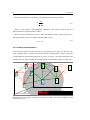
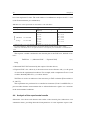
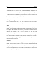
The first prototype of MScMS is made by the following elements:
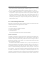
• Cricket constellation. 22 Cricket devices have been freely distributed around a measuring area, covering a volume of about 60 m3. To make their positioning easy, we used
different supports, such as booms, articulated arms and tripods (see Fig. 3.1).
wireless devices, distributed
around the working area
data sent to PC
via Bluetooth
mobile probe
measured object
Fig. 3.1. Practical application of MScMS
PC
24
Chapter 3
• Mobile probe. It is made by a rigid structure containing the following elements:
-
two Cricket devices;
-
a tip to “touch” the points of measured objects. Tip (V) and Cricket devices (A and
B) are aligned and spaced as indicated: d(A−B) = 450 mm e d(A−V) = 540 mm (see
Fig. 3.2);
-
a Bluetooth transceiver connected with one of the two Cricket devices, by a RS232
serial port.
V
A
B
90 mm
Bluetooth
transceiver
450 mm
trigger mounted
on device A
Fig. 3.2. Mobile probe prototype
• Personal computer. An ad hoc application software runs on a standard PC. To receive
data sent by the probe, the PC is equipped with a Bluetooth transceiver.
• Application software. The purpose of this software is to drive the user through measurements and to make results display efficient. Functions provided are similar to those
typically implemented by CMM software packages. MScMS, likewise CMMs, makes
it possible to determine the shape/geometry of objects (circumferences, cylinders,
plans, cones, spheres etc..), on the basis of a set of measured surface points gathered
from the mobile-probe, using classical optimization algorithms [Overmars, 1997].
More in detail, the software is organized into three application modules to assist the
user in the following operations:
-
Initialization. This is a guided procedure to switch on wireless devices (Crickets and
Bluetooth adapter), and open the PC connection for data reception from the mobile
probe.
-
Semi-automatic localization of the constellation. This procedure is described in Section 2.4.4.
MScMS prototype
-
25
Measurements. Execution of different kinds of measurement: single points measurements, distance measurements, curves and surfaces evaluation (see Fig. 3.4 and
Fig. 3.5).
(a)
(b)
Fig. 3.3. MScMS software menu
Fig. 3.3, Fig. 3.4 and Fig. 3.5 show some displays of the MScMS software.
Single Points Measurements
[mm]
[mm]
[mm]
[mm]
[mm]
x = 1000 ; y = 2000 ; z = 1000
[mm]
Fig. 3.4. Display for the measurement of single points
[mm]
26
Chapter 3
Measurements are taken like this: when the probe trigger is pulled, the application
software calculates Cartesian coordinates of the point touched by the probe tip. If measurement is correctly taken, an acoustic signal is emitted. Measure results are displayed using numeric and graphical representations. Fig. 3.3 shows some screenshots of the software main menu and sub-menus.
Function to determine a circumference on a horizontal
plane ( points minimum )
Center :
( x = 1122 mm; y = - 40 mm)
Radium :
219 mm
σx
σy
=
=
13 mm
13 mm
Fig. 3.5. Display for the measurement of a circle
3.3 MScMS actual performance, critical aspects and possible
improvements
A preliminary prototype of MScMS has been set-up and tested, with the purpose of verifying system feasibility and to evaluate its performance. The prototype actual performance has been estimated carrying out two practical tests:
• Repeatability test. Repeatability is defined as: "closeness of the agreement between the
results of successive measurements of the same measurand, carried out under the same
conditions of measurement” [GUM, 2004; VIM, 2004]. In this test, a single point
within the working volume is measured repeating the measurement about 50 times,
leaving the mobile-probe in a fixed position (see Fig. 3.6-a). The test is repeated measuring at least 20 different points in different areas of the working volume. For each
point, we have calculated the standard deviations (σx, σy, σz) related to the registered
Cartesian coordinates (x, y, z).
MScMS prototype
27
• Reproducibility test. Reproducibility is defined as: “closeness of the agreement between the results of successive measurements of the same measurand, carried out under
changed conditions of measurement” [GUM, 2004; VIM, 2004]. This test is similar to
the previous one, with the only difference that the mobile-probe orientation is changed
before each measurement, with the aim of approaching each (single) point from a different direction (see Fig. 3.6-b).
measured (single) point
a) repeatability: the mobile-probe position and orientation
are the same in the different measurements
b) reproducibility: the mobile-probe direction is
changed before every measurement
Fig. 3.6. Representation scheme of the practical tests carried out to evaluate MScMS performances
The statistical results of these preliminary tests are reported in Tab. 3.1.
Tab. 3.1. Results of the MScMS preliminary tests
Test
Mean standard
deviation [mm]
σx
4.8
repeatability
σy
5.1
σz
3.5
σx
7.3
reproducibility
σy
7.8
σz
4.1
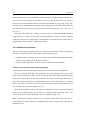
Let notice that σz value is basically lower than σx and σy, both for repeatability and reproducibility tests. This behaviour is due to the geometric configuration of the constellation devices: in general, network devices are mounted on the ceiling or at the top of the
measuring area; for this reason, they can be considered as approximately placed on a
plane (XY) perpendicular to the vertical (Z) axis (see Fig. 3.1).
Since we have experimentally verified that the distribution of the point coordinates can
be considered to be normal, both for repeatability and reproducibility data, the variability
range, considering a 99.73% confidence level, is given by ±3σ [Montgomery, 2008].
Reproducibility range is an index of the instrument actual accuracy, whereas repeatability variation range is an index of the target instrument accuracy, supposing to compensate the most important causes of systematic errors.
28
Chapter 3
The most critical aspects of the whole measuring system are due to US sensors. In particular:
1. Dimensions of US transceivers;
2. Different types of noise affecting US signals;
3. Speed of sound dependence on environmental conditions;
4. Working volume discontinuities;
5. Use of amplitude threshold detection at receivers.
These aspects are individually discussed in the following subsections.
Dimensions of US transceivers
A source of uncertainty in US time-of-flight measurements is due to non punctiform US
sensors. The volume of each piezo-electric crystal is about 1 cm3. As shown in Fig. 3.7, it
is difficult to determine the exact point of departure/arrival of a US signal exchanged between a pair of Crickets. These points are placed on the US sensors surfaces, and may
vary depending on their relative position.
(a)
≈1.2 cm
(b)
ultrasound points of departure/arrival
Fig. 3.7. Points of departure/arrival of US exchanged between 2 Crickets
Regarding the future, Cricket devices will be modified in order to minimize this problem, for example by miniaturizing the US sensors.
Different types of noise affecting US signal
During measurements, the user should not obstruct US signal propagation. Two possible
drawbacks may occur:
MScMS prototype
29
• transmitted US signal does not reach the receiver because it is completely shielded by
an obstacle;
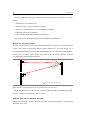
• transmitted US signal diffracts and goes round the interposed obstacle, reaching the receiver. In this case, path covered by US is longer than the real distance between transmitter and receiver (see Fig. 3.8).
obstacle
US transmitter
US receiver
target distance
measured distance due to diffraction
Fig. 3.8. US diffraction
The second case is more complicated to manage than the first. In general, it is not easy
to notice possible path deflections. Probe can be prone to other types of noise, like external sources of US. For example, US produced by metal objects jingling. However, wrong
distance measurements, like the ones described, can be indirectly detected and rejected.
To that purpose, an effective diagnostic tool is the Error Function (EF, see Eq. 2.4)
[Franceschini et al., 2002; Franceschini et al., 2007-II]. This function, evaluated during
the localization of both the mobile-probe devices (A and B), is an index of the bias between measured distances (evaluated by means of US transceivers) and calculated distances (determined on the basis of the localised position). We have experimentally verified that the minimum value of the EF is generally of the order of the tenth of mm2. When
one or more measured distances are wrong – due to systematic effects – the EF minimum
value “explodes” becoming 3 or 4 orders of magnitude greater. In practical terms, during
the location of devices A and B, if the EF minimum is included below a threshold value
(say 70 mm2), then the position is considered to be reasonable. Otherwise, it is rejected.
Speed of sound dependence on environmental conditions
Speed of sound (s) value makes it possible to turn US time of flight into a distance (Eq.
2.2). It is well known that the speed of sound changes with air conditions – temperature
and humidity – which can exhibit both temporal and spatial variations within large working volumes. As a consequence, (s) requires to be often updated, depending on the time
and the position. A partial solution to this problem is to use the temperature (T) information evaluated by embedded thermometers at the Cricket receivers and to periodically up-
30
Chapter 3
date (s) using an experimental relation s = s(T) [Bohn, 1988]. As a better alternative, we
implemented an optimization procedure which makes it possible to estimate, measurement by measurement, the optimum (s) value, using the following information:
• times of flight among (at least) 4 constellation Crickets and the 2 mobile-probe Crickets (A and B);
• a standard of length for referability, given by the a priori known distance between the
mobile-probe Crickets (A and B).
By an automatic optimization, we calculate the (s) value which better satisfies the previous constraints, with reference to a particular portion of the working volume. In this
way, the (s) value can be recalculated for each single measurement.
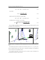
Working volume discontinuities
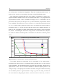
A requirement of the measuring instruments is to measure uniformly and with no discontinuities all the points within the working volume. Due to its technology, MScMS is
based on a network of distributed devices, communicating through RF and US. While RF
sensors communication range is almost omni-directional and up to 25 m, US sensors have
a communication range limited by “cones of vision” with an opening angle of about 170°
and a range of no more than 6-8 m (see Fig. 3.9). Signal strength outside the cones drops
to 1% of the maximum value (see the radiation pattern in Fig. 4.3) [Priyantha et al.,
2000].
D4
D1
D2
D3
≈ 170°
“cone of vision” of
network device D2
ceiling
“cone of vision” of
network device D3
MScMS prototype
31
Fig. 3.9. Representation scheme of the US sensors "cones of vision"
It is therefore important to provide a full coverage to the area served by constellation
devices by proper alignment of the US transmitters towards the measuring area. To
increase the working volume coverage it is necessary to increase the number of
constellation devices. In general, the best solution is mounting the constellation devices
on the ceiling or at the top of the measuring area, as shown in Fig. 3.1.
On the basis of practical tests, we determined that the coverage of a indoor working
volume about 4 meters high can be achieved using about one constellation device per
square meter (considering a plant layout).
Use of amplitude threshold detection at receivers
To evaluate time-of-flight (TOF), receivers can detect signals with amplitude equal or
greater than a threshold value. Since US transceivers operate at 40 kHz frequency, the
time period of a complete wave cycle is 1/40,000 s = 25 μs. US waves are saw-tooth
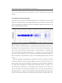
shaped, with a linear rise (see Fig. 3.10).
Considering fresh US signals at the transmitter, their amplitude may decrease depending on two basic factors:
• (distance) attenuation: signal amplitude decreases depending on the distance covered.
• transmitter orientation: since US transmitters are not omni-directional, signal amplitude changes depending on their orientation. In particular, the maximum signal
strength is related to the direction perpendicular to the transducer surface (at the axis of
the “cone of vision”), while signal amplitude drops to 1% of the maximum value at
±40° away from it (see Fig. 3.3) [Priyantha et al., 2000].
The consequence of the use of amplitude threshold detection is the occurrence of errors in
TOF evaluation. The implementation of the threshold detection method at the receivers is
a source of inaccuracy. As represented in Fig. 3.10 and Fig. 4.4, the signal transient time
at the receiver strongly influences the ranging precision. This may cause relatively large
errors in the TOF evaluation (one ore more US time periods).
Actually, since the speed of sound is about 340 m/s, one US time period corresponds to a
distance of about 8.5 mm. Considering that the threshold can be exceeded even 4 period
late, distance overestimation can be up to 3÷4 cm!
32
Chapter 3
signal amplitude
errors in TOF
full amplitude signal
signal with decreased amplitude
amplitude threshold
(set at the receiver)
T= 25 μs
time from the arrival of the
first US signal at the receiver
Fig. 3.10. Representation scheme of the error produced by the use of amplitude threshold detection
method. The signal transient time at the receiver strongly influences the ranging precision
3.4 Final considerations
MScMS first prototype is adaptable to different working environments and does not require long installation or start-up times. Before performing measurements, constellation
devices − freely distributed around the measuring area − automatically locate themselves
in few minutes. System is supported by an ad hoc software − created in Matlab − to drive
the user through measurements and online/offline elaborations.
Today, MScMS Achilles’ heel is represented by its low accuracy (few centimetres) related to the measured points position. This is mainly due to the use of US transceivers
(implementation of the threshold signal detection method, non punctiform dimension,
speed of sound dependence on temperature etc..). As research perspectives, all factors affecting system accuracy will be analysed and improved in detail, in order to reduce their
effect.
4.
Experimental evaluation of the MScMS ultrasound
transducers
4.1 Introduction
Ultrasonic (US) sensors are used in many application fields. In general, the main features
of ultrasound transducers change depending on the propagation medium (solids, liquids,
air). One of the most important applications of US transducers is distance measurement,
where the propagation medium of the acoustic signals is typically air. Common applications associated with distance measurement are presence detection, identification of objects, measurement of the shape and the orientation of workpieces, collision avoidance,
room surveillance, liquid level and flow measurement [Delpaut et al., 1986]. Ultrasonic
ranging systems are traditionally low cost, compared to other technologies like the optical
laser based. Unfortunately, they are also characterized by low accuracy, low reliability
due to reflections of the transmitted signals, and limited range [Manthey et al., 1991]. US
sensors provide high accuracy only in certain working contexts. Excellent performances
can be achieved when measuring for example short, fixed distances and controlling environmental conditions (temperature and humidity). The most common technique for distance evaluation is by measuring the time-of-flight (TOF) of the US signal – either from a
transmitter to a receiver or using a single transceiver, which transmits the US signal and
receives the corresponding reflected signal. Other aspects influencing the performance of
ultrasonic sensors are the type of transducers and the signal detection method used (i.e.
thresholding, envelope peak, phase detection – discussed in Section 4.2). For this reason,
different types of transducers can be employed depending on the specific application.
Most of commercially available air ultrasonic transducers are ceramic based and operate
at 40 kHz. Transducers that operate at higher frequencies, such as at 200 kHz, are more
limited and more expensive [Toda, Dahl, 2006].
This chapter focuses on the US transducers used by the Mobile Spatial coordinate
Measuring System (MScMS). The characterization of the MScMS’ US transceiver is
performed by means of several experiments, organically designed through a factorial
34
Chapter 4
plan, and performed in different measuring conditions. Particular emphasis is given to the
effect of the US signal attenuation on the TOF estimation. Also, the major sources of
errors in TOF evaluation are investigated in a structured way, by means of an
experimental factorial plan. The results of this analysis can be useful to identify the major
MScMS sources of inaccuracy and to determine how the error in TOF evaluation changes
in the different points within the Cricket transmitters’ “cones of vision” (see Fig. 3.9).
The chapter is organised in four sections. Section 4.2 describes the main features of
piexo-electric US transceivers, like those equipping MScMS. Section 4.3 provides a
detailed description of the factorial plan, analysing the effects and the possible
interactions of the sources of attenuation. Section 4.4 presents and discusses the results of
the factorial plan. Finally, the conclusions and future direction of this research are given
in Section 4.5.
4.2 Piezo-electric US transducers
In modern ultrasonic distance measurement systems for industrial applications, piezoelectric transducers clearly dominate. Typical advantages are their compact, rugged mechanical design, high efficiency, great range of operation temperature and relatively low
cost. Airborne ultrasound systems have been developed for many types of distance measurement using two possible techniques [Berners et al., 1995]:
• pulse-echo: a transducer emits a burst of US, which bounces off any object in the path
of the beam. The transducer then acts as a receiver for the reflected signal. A measurement of the time delay from transmission to reception determines the distance to the
target.
• time-of-flight: a separate transmitter is pointed towards the receiver. Instead of relying
on reflections, this system detects the direct transmission of the signal from transmitter
to receiver. After measuring the TOF, the sensors distance can be calculated knowing
the speed of sound value.
Cricket devices, being equipped with either a US transmitter and a receiver, implement
the TOF technique.
A complex problem when using US transducers is the choice of the characteristic parameters (typically, resonant frequency and bandwidth). For distance measurement with
relatively high precision (few millimetres), transducers with a wide bandwidth are
Experimental evaluation of the MScMS ultrasound transducers
35
needed. Bandwidth is a measure of how rapidly a signal reaches the steady state. A signal
at the receiver – obtained from transducers with a small bandwidth – climbs slowly from
its beginning to its peak in time-domain, causing a relatively large transient time at the
receiver. This behaviour is shown in Fig. 7 [Cheng, Chang, 2007; Tong et al. 2004].
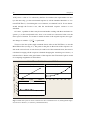
A second factor affecting measurement accuracy is the transducer resonant frequency.
With increasing frequency (and thus reducing wavelength) a better resolution is achievable. Unfortunately, both the transducer bandwidth and resonant frequency are directly
correlated with the US attenuation and – consequently – they limit the detection range. In
other terms, considering the same US signal amplitude, the radiated signal amplitude at a
given distance from the transmitter becomes smaller if its bandwidth and resonant frequency increase [Tong et al., 2005; Kazys et al., 2007]. For this reason, the selection of
ultrasonic frequency and bandwidth is a compromise between accuracy and detection
range.
The piezo-electric transducer adopted by Cricket devices is a low-cost, general purpose
model (Murata MA40S4R, see Fig. 4.1-a), with a relative wide bandwidth (see Fig. 4.1b), in which the centre frequency is about 40kHz. This working frequency is a trade-off
between accuracy (considering the single distances, it is around 1-2 centimetres) and detection range (up to 6-8 meters) [Balakrishnan et al., 2003].
The acoustic strength of the radiation from a flat transducer with “piston motion” (like
the Crickets’ US transducers) is generally angle dependent because of the phase difference of waves from each point on the surface. Actually, the acoustic radiation is the integral sum of the waves from all points on the transmitter surface, and the propagation path
difference from each point to a reference observation point has a phase cancellation effect
which leads to signal attenuation [Lamancusa, Figueroa; 1990]. However, if the receiver
is directly facing the transmitter at sufficient distance from it, the acoustic radiation from
each point of the transducer surface does not have a phase-cancelling effect. This because
the distance from an arbitrary point on the transmitter surface to the receiver becomes almost constant, and the difference is much smaller than the wavelength [Toda, 2002]. On
the other hand, if the transmitter is misaligned with the receiver, the US signal amplitude
will be attenuated because of the disruptive interference of the different US signals from
the transmitter different surface points. This effect is represented by the simplified
scheme in Fig. 4.2. This scheme considers the interaction of the waves from two points
on the transducer surface; the same principle can be extended to all the surface points.
36
Chapter 4
(a)
(b)
Fig. 4.1. (a) internal construction of a Murata MA40S4R piezo-electric ultrasonic transmitter/receiver. The dimensions of the piezo material causes the disk to resonate at a precise frequency (around 40kHz); (b) representation of the transmitter bandwidth by means of a frequency
response plot
Receiver
(faces aligned)
Transmitter
Transmitter
pt 1
pt 1
pt 2
pt 2
θ
resulting wave
(full amplit ude)
(a)
Receiver
(misaligned)
(b)
Fig. 4.2. US signal strength dependence on the transmitter angle (θ). The simplified scheme represents the interaction of the waves from 2 points on the transducer surface. The resulting wave is
given by the sum of the single waves. If the receiver is directly facing the transmitter (case-a) the
two individual waves are in-phase and the resulting wave amplitude has the maximum value. If the
transmitter is misaligned with the receiver (case-b) the resulting wave is attenuated because of a
phase cancelling effect due to the phase difference between the two individual waves [Lamancusa,
Figueroa; 1990]
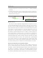
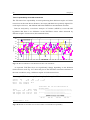
The resulting ultrasonic transmitter radiation pattern, depending on the transmitter misalignment angle with the receiver, is shown in Fig. 4.3. As represented, the transmitter US
signal strength drops along directions that are away from the direction facing the ultrasonic transducer.
Similarly, the received signal strength can be influenced by the receiver orientation. In
particular, considering the same signal strength from the transmitter, the received signal
strength is maximum when the receiver’s surface is facing the transmitter. On the other
hand, the received signal decreases when the receiver’s surface is angled.
Experimental evaluation of the MScMS ultrasound transducers
37
Fig. 4.3. The radiation pattern of the Cricket ultrasonic transducer on a plane along its axis, depending on the orientation. Signal strength drops along direction that are away from the normal
direction to the transducer surface
Several signal methods have been developed for detecting US signals:
Thresholding. It is the simplest and the most widely used, and applies to any type of short
duration signal. By this method, implemented by Cricket devices, the receiver electric
output signal is compared with a threshold level (65 mV for Cricket devices), such that
arrival of the wave is acknowledged when the signal reaches this level. This method depends on the amplitude of the pulse received: the larger the signal amplitude, the smaller
the time taken by the signal before reaching the threshold. Considering the example in
Fig. 4.4, when the signal has a full amplitude, the detection threshold is first exceeded by
the second peak of the US waveform. When the waveform is attenuated by a factor of 0.5
(half amplitude signal), the detection threshold is first exceeded by the third peak of the
US waveform. If the channel attenuation is quite significant, it may cause the threshold to
be exceeded a few periods late, instead of just one period late. Considering that, for a
40kHz US a period is 25 μs, this error will approximately be in integer multiples of 25μs.
Since the speed of sound is around 340 m/s, a one period error corresponds to a
25·340/1000= 8.5 mm distance overestimation. In practice, since the threshold can be exceeded even 4 period late, distance overestimation can be up to 3÷4 cm!
Envelope peak detection. It is a modification of thresholding, which may be called adjustable thresholding. This method acknowledges arrival of the signal when a maximum amplitude is detected. Therefore, it does not depend upon the absolute magnitude of the
pulse, but only upon its shape. As a consequence it is more accurate and robust than simple magnitude thresholding, where the acknowledge time can easily jump by one period.
Phase-detection. Other more refined ranging methods are based on phase detection with
fixed-frequency signals and with frequency-modulated signals. These methods, however,
requires complex hardware and software. They use a digital signal processor to process
38
Chapter 4
the phase measurements and overcome the inherent range limitation of one wavelength
[Manthey et al., 1991; Tong et al., 2001].
Transient time at the receiver
Receiver (electric) output signal [mV]
240
180
3rd peak
120
2nd peak
detection threshold
60
1st peak
0
-60
-120
-180
half amplitude signal
full amplitude signal
-240
Time from the arrival of the first US signal at the receiver [μs]
Fig. 4.4. Schematic representation of thresholding detection. A minimum number of cycles are
necessary to bring the receiver to steady state conditions (transient time at the receiver) [Johansson
et al., 2005]. The error in the distance measurement is dependent on the received US signal amplitude, because the time taken for the received signal to reach the threshold is dependent on it
4.3 Factors affecting US transceivers
MScMS measurement accuracy may change depending on many different factors related
to the use of US transceivers, such as temperature, humidity, air turbulence, transducers
geometry, transducer bandwidth, US signal attenuation etc. When implementing a thresholding detection method, the major effects are due to the factors related to the US signal
attenuation. The most important sources of attenuation are [Franceschini et al., 2008-II;
MIT C.S.A.I.L., 2004]:
• transceivers distance;
• transceivers misalignment angle;
• transducer battery charge level.
With the aim of organically investigating the effect of these factors on TOF measurements, a complete experimental factorial plan is built.
Fig. 4.5 shows a representation scheme of the experimental setup:
Experimental evaluation of the MScMS ultrasound transducers
39
• transmitter and receiver are positioned facing each other;
• transceivers distance are positioned at known distance (1st factor);
• transmitter face is not perfectly aligned with receiver face. A misalignment angle (θ)
with regard to the transmitter face is introduced (2nd factor). On the other hand, the receiver face is perpendicular to the US waves direction of propagation;
• transmitter battery charge level is monitored measuring the battery potential difference
(3rd factor). Each Cricket is equipped with two AA rechargeable 2700 mAh batteries,
connected in series. Their potential difference is measured by a standard voltmeter. The
potential difference is not a direct measurement of the battery charge level, but – since
they are correlated – it is an useful indicator of it [Franceschini et al., 2007-I].
Transmitter
V
rd
(3 factor)
Receiver
US
θ (2
nd
factor)
d (1st factor)
Fig. 4.5. Experimental setup
TOF is measured changing these 3 factors at different levels:
• Seven levels for θ (transmitter rotations from 0° to 60° in 10° intervals). For larger angles, transmitter and receivers do not easily communicate, due to the strong decrease in
the US signal strength (see Fig. 6).
• Three levels for d: short, medium and long distance between transceivers. These distances have been measured using 3 reference bars, accurately calibrated using a standard Coordinate Measuring Machine (accuracy lower than a hundredth of mm) [Furutani and Kamahora, 2001].
• Five levels for V (from 2.3V to 2.7 V in 0.1 V intervals).
Tab. 4.1 provides a summary of the combinations for the three factor levels.
There are 7∙3∙5 = 105 different combinations to be carried out. According to the factorial plans good practice, measurements are randomized [Montgomery, 2008]. For each of
these combinations, 50 measurements of the TOF are performed. All the experiments
40
Chapter 4
have been replicated 5 times. The total number of combinations analysed is 105∙5 = 525
(with 50 measurements per combination).
Tab. 4.1. List of the experiments on the Cricket’s US transducers
1st – Transceivers distance (d)
Factors
2nd – Transmitter misalignment
angle (θ)
3rd – Battery level (V)
θ1 = 0°
V1 = 2.7 V
θ2 = 10°
V2 = 2.6 V
θ3 = 20°
(Medium) d2 = 2034 mm
V3 = 2.5 V
θ4 = 30°
V4 = 2.4 V
θ5 = 40°
(Long)
d3 = 3671 mm
V5 = 2.3 V
θ6 = 50°
θ7 = 60°
- all the possible 7∙3∙5 = 105 different combinations are carried out in random order;
- for each combination, TOF measurements are repeated 50 times and the average value is taken;
- all the 105 combinations above are replicated 5 times. Consequently, the total number of combinations is
525.
d1 = 1160 mm
Levels
(Short)
The response variable considered in the factorial plan is the TOF error, defined as follows:
TOF-Error = (Measured-TOF – Expected-TOF)
(4.1)
being
• Measured-TOF: TOF measured by the couple of Cricket devices;
• Expected-TOF = d/s: where (d) is the transceivers known distance and (s) is the speed
of sound in the experimental conditions. For example, with a temperature T=24 °C and
a relative humidity RH=27%, (s) is about 346 m/s.
TOF-Error is used as an indicator of the inaccuracy in TOF evaluation [Franceschini et
al., 2007-I].
The experiments are performed in a controlled environment (T=24°C and RH=27%) to
prevent outlier distance measurements due to reflected ultrasonic signals or to variations
in the environmental conditions.
4.4 Analysis of the experimental results
Subsection 4.4.1 shows and discusses the results of the factorial plan. Subsection 4.4.2
summarizes them, providing theoretical interpretations of some important aspects. Sub-
Experimental evaluation of the MScMS ultrasound transducers
41
section 4.4.3 presents other minor experiments, aimed at deepening the factorial plan
analysis.
4.4.1 Results of the factorial plan
Analysing the factorial plan experimental outputs, the first interesting result is that the
TOF-Error standard deviation (σ) changes depending on the TOF-Error value. In other
words, the population of TOF-Error cannot be considered as homoscedastic, that is to say
with a constant standard deviation.
Fig. 4.6. TOF-Error standard deviation vs average TOF-Error. For each of the 525 factors combinations, variables are calculated using the corresponding 50 individual TOF-Error measurements.
This behaviour is well shown on Fig. 4.6, where for each of the 525 factorial plan combinations, the average TOF-Error and the respective standard deviation – calculated using
the corresponding 50 individual measurements – are plotted. It can be noticed that the
larger the average TOF-Error value, the larger the individual measurements dispersion.
The non constancy of the TOF-Error variance is also tested through the Levene’s statistical test.
Since the assumption of homogeneity of TOF-Error variances is violated, the Analysis
of Variance (ANOVA) cannot be properly applied, in order to verify if factors have a significant effect on the response (TOF-Error) and if there are factor interactions [Montgomery, 2008]. The usual approach to dealing with nonconstant variance is to apply a variance-stabilizing transformation. In this approach, the conclusions of the analysis of
variance will apply to the transformed populations. The most common transformation is
the exponential y*=yλ, where λ is the parameter of the transformation. Box and Cox proposed an optimization method for determining the transformation parameter [Box et al.,
42
Chapter 4
1978]. Once a value of λ is selected by the Box-Cox method, the experimenter can analyse the data using y as the transformed response (it will be identified hereafter as “corrected TOF-Error”). Considering the case of interest, we obtained λ=0.52. It was demonstrated through the Levene’s test, that the transformed response variance is now
stabilized.
Of course, a problem is that it may be uncomfortable working with the transformed response (y*) in the transformed scale, since it can result in a nonsensical value over the
factor space of interest. To construct a model in terms of the original response, the oppo1
site change of variable – ( y*) λ – is performed.
To have a first idea of the single examined factors effect on the TOF-Error, we use the
Main Effects Plot (see Fig. 4.7). The points in the plot are the means of the response variable at the various levels of each factor (for each level of the examined factor, the mean is
calculated averaging all the responses obtained changing the remaining two factors). A
reference line is drawn at the grand mean of the response data. This kind of plot is useful
for comparing magnitudes of main effects.
Mean
corrected TOF-Error
Main Effects Plot for Corrected TOF-Error
14
12
10
8
1160
2034
3671
0
10
20
30
40
50
60
V
V [Volts]
16
corrected TOF-Error
θ [degrees]
theta
d [mm]
d
16
14
12
10
8
2,3
2,4
2,5
2,6
2,7
Fig. 4.7. Main effect plot for means, related to the three examined factors: θ (misalignment angle),
d (transceivers distance), V (batteries potential difference)
Experimental evaluation of the MScMS ultrasound transducers
43
The qualitative result is that misalignment angle and transmitters distance have an important effect, while the effect of battery charge level is minor.
In order to qualitatively judging the presence of interactions among the three factors,
an Interaction Plot is constructed in Fig. 4.8. This plot represents the means for each level
of a factor with the level of a second factor held constant (considering two factors, for
each combination of their levels, the mean is calculated averaging the responses obtained
changing the remaining factor). Interaction between two levels is present when the response at a factor level depends upon the level(s) of other factors. Parallel lines in an interactions plot indicate no interaction. The greater the departure of the lines from the parallel state, the higher the degree of interaction [Montgomery, 2008].
Interaction Plot for Corrected TOF-Error
Data Means
0
10
20
30
40
50
60
2,3
2,4
2,5
2,6
2,7
corrected TOF-Error
20
15
d [mm]
1160
2034
3671
10
20
corrected TOF-Error
θ [degrees]
15
10
θ [degree]
theta
0
10
20
30
40
50
60
V [Volts]
Fig. 4.8. Interaction plot for Corrected TOF-Error, considering the three factors (d, θ, V)
The qualitative result is that misalignment angle and transmitters distance have an important effect, while the effect of battery level is minor, but not irrelevant.
Both the factors effect end their interactions are quantitatively examined by performing
an Analysis of Variance (ANOVA) (see Fig. 4.9). In the ANOVA, the variance related to
the response is partitioned into contributions due to the different factors and their interactions. Results of an ANOVA can be considered reliable as long as the following assumptions are met: (1) response variable is normally distributed, (2) data are independent, (3)
44
Chapter 4
variances of populations are equal. After applying the Box-Cox response transformation,
all these assumptions are satisfied.
Analysing the ANOVA results (Fisher’s test), it can be sentenced that all three factors
are significant and their interactions as well. With regard to the effect of the single factors, the most important are d and θ, while the effect of V is minor (small F value). This is
consistent with the Main Effect Plot of Fig. 4.7. With regard to the factors interactions,
they are all statistically significant (small p-values), but very weak. The strongest is the
one between d and θ.
General Linear Model: corrected TOF error versus d; θ; V
Factor
d
θ
V
Type
fixed
fixed
fixed
Levels
3
7
5
Values
1160; 2034; 3671
0; 10; 20; 30; 40; 50; 60
2.3; 2.4; 2.5; 2.6; 2.7
Analysis of Variance for corrected TOF error
Source
d
θ
V
d*θ
d*V
θ*V
Error
Total
single factors effect
interactions between
couples of factors
DF
2
6
4
12
8
24
468
524
Seq SS
4071.35
2368.87
44.22
121.55
18.09
30.15
46.36
6700.59
Adj SS
4071.35
2368.87
44.22
121.55
18.09
30.15
46.36
Adj MS
2035.67
394.81
11.06
10.13
2.26
1.26
0.10
F
20551.49
3985.88
111.61
102.26
22.83
12.68
P
0.000
0.000
0.000
0.000
0.000
0.000
Fig. 4.9. ANOVA applied to the (transformed) response of the factorial plan
Surface Plot of TOF-Error vs d and θ
300
200
TOF-Error
[μm]
100
0
4000
3000
d [mm]
2000
1000
0
20
40
60
θ [degrees]
Fig. 4.10. Surface plot to represent the effect of the interaction of factors d and θ on the TOF-Error
Experimental evaluation of the MScMS ultrasound transducers
45
The effect of this interaction on the TOF-Error is represented by the surface plot in Fig.
4.10. As shown, the composition of large misalignment angles (θ) and large distances (d)
produces TOF-Errors which are larger than the these obtained adding the effects of the
single factors, taken separately.
Another representation of the experimental outputs is given by Fig. 4.11, where the average-TOF-Error and the corresponding standard deviation (calculated for each combination of factors using the 50 repeated measurements) are plotted depending on V and θ, for
each of the 3 transceivers distances.
Average TOF Vs Misaligment Angle (d1 = 1160 mm)
350
TOF-Error Standard Deviation [μs ]
2.5 V
2.4 V
250
2.7 V
24
2.6 V
300
Average TOF-Error [μs ]
TOF Standard Deviation Vs Misaligment Angle (d1 = 1160 mm)
26
2.7 V
2.3 V
200
150
100
50
0
2.6 V
22
2.5 V
20
2.4 V
18
2.3 V
16
14
12
10
8
6
4
2
0
10
20
30
40
50
Misalignment Angle [degrees]
60
70
0
2.6 V
2.5 V
2.4 V
250
2.3 V
200
150
100
50
0
70
2.6 V
22
2.5 V
20
2.4 V
18
2.3 V
16
14
12
10
8
6
4
2
0
10
20
30
40
50
Misalignment Angle [degrees]
60
0
70
Average TOF Vs Misaligment Angle (d3 = 3671 mm)
350
20
30
40
50
Misalignment Angle [degrees]
60
70
2.7 V
24
TOF-Error Standard Deviation [μs ]
2.6 V
2.5 V
2.4 V
250
10
TOF Standard Deviation Vs Misaligment Angle (d3 = 3671 mm)
26
2.7 V
300
Average TOF-Error [μs ]
60
2.7 V
24
TOF-Error Standard Deviation [μs ]
Average TOF-Error [μs ]
26
2.7 V
300
20
30
40
50
Misalignment Angle [degrees]
TOF Standard Deviation Vs Misaligment Angle (d2 = 2034 mm)
Average TOF Vs Misaligment Angle (d2 = 2034 mm)
350
10
2.3 V
200
150
100
50
0
2.6 V
22
2.5 V
20
2.4 V
18
2.3 V
16
14
12
10
8
6
4
2
0
10
20
30
40
50
Misalignment Angle [degrees]
60
70
0
10
20
30
40
50
Misalignment Angle [degrees]
60
70
Fig. 4.11. TOF average value and standard deviation depending on the misalignment angle (θ) and
the battery level (V), for different transceivers distances
46
Chapter 4
As already noticed, TOF-Error increases depending on θ and d. Also, the TOF standard
deviation is slightly increasing with the angle; this behaviour is more definite for large
distances between transmitter and receiver.
With respect to the experimental data, in Fig. 4.11 there are some measurements not
included in the factorial plan. They are TOF-Error measurements related to misalignment
angles of 70 degrees, which cannot be performed for all the possible distances. For instance, considering the long transceivers distance (d3=3871 mm), transmitter and receiver
are not able to communicate because of the strong signal attenuation. It can be noticed
that the effect of the two most significant factors (θ and d) on the TOF-Error is evident,
while the effect of the battery charge level (V) is very small, compared to the previous
two. TOF-Error is always positive, because of the TOF overestimation due to the signal
attenuation (which is proportional to d, θ, and V). The effect of the transceivers distance
on the TOF-Error is also well shown in Fig. 4.12, plotting the TOF-Error versus the
transceivers distance for different misalignment angles.
350.0
TOF-Error [ μ s ]
300.0
250.0
200.0
TOF-Error vs Transceivers Distance (d)
00 degrees
10 degrees
20 degrees
30 degrees
40 degrees
50 degrees
60 degrees
150.0
100.0
50.0
0.0
1000
1500
2000
2500
3000
Transceivers Distance (d) [m m ]
3500
4000
Fig. 4.12. TOF-Error depending on the transceivers distance (d). The plotted curves are related to
different transmitter misalignment angles (θ). The effect of the signal attenuation (TOF overestimation) increases with the transceivers distance
The most interesting considerations related to the factorial plan experiments are discussed and interpreted in Subsection 4.4.4.
Linear regression model
Considering the results of the factorial plan, we constructed a linear regression model representing the relationship among TOF-Error and the three factors d, θ and V. Such a
model can be useful for providing some indications on the TOF-Error expected value, de-
Experimental evaluation of the MScMS ultrasound transducers
47
pending on d, θ and V. In order to evaluate the factors interaction, but not to complicate
too much the analysis, we chose a 2nd order polynomial model such as:
TOF-Error = C1 + C2 ∙ d + C3 ∙ θ + C4 ∙ V + C5 ∙ d2 + C6 ∙ θ2 + C7 ∙ V2 + C8 ∙ d ∙ θ
(4.2)
+ C9 ∙ d ∙ V + C10 ∙ θ ∙ V
With the support of the Minitab best regression tool, we constructed a model, which
best fits experimental results (see Fig. 4.13). All the terms in Eq. 4.2 are considered to be
significant, except C7∙V2 (quadratic effect of factor V) and C10∙(θ∙V) (interaction between
factors θ and V).
Best Subsets Regression: TOF error versus d; θ; V; d ; θ2; V ; d·θ; d·V; θ·V
2
Response is
Vars
R-Sq
No.
1
80.9
1
53.5
1
51.8
2
90.1
2
89.5
2
89.4
3
92.2
3
91.2
3
91.0
4
95.7
4
95.4
4
95.1
5
96.2
5
95.9
5
95.9
6
96.4
6
96.2
6
96.2
7
96.4
7
96.4
7
96.4
8
96.4
8
96.4
8
96.4
9
96.4
TOF error
R-Sq Mallows
(adj)
Cp
80.9 2219.3
53.4 6163.3
51.7 6407.8
90.0
907.8
89.4
994.3
89.4 1002.7
92.1
607.0
91.1
749.6
90.9
778.3
95.6
107.1
95.3
149.4
95.1
185.4
96.1
36.4
95.9
73.8
95.9
73.8
96.3
10.0
96.2
33.2
96.2
33.2
96.4
6.7
96.4
6.7
96.4
8.2
96.4
8.0
96.4
8.0
96.4
8.7
96.4
10.0
S
30.621
47.824
48.691
22.117
22.777
22.840
19.649
20.857
21.093
14.632
15.121
15.525
13.764
14.224
14.224
13.416
13.711
13.712
13.361
13.361
13.380
13.364
13.364
13.374
13.377
d
θ
V
d2
2
θ2
V2 d·θ d·V θ·V
X
X
X
X
X
X
X
X
X
X
X
X
X
X
X
X
X
X
X
X
X
X
X
X
X
X
X
X
X
X
X
X
X
X
X
X
X
X
X
X
X
X
X
X
X
X
X
X
X
X
X
X
X
X
X
X
X
X
X
X
X
X
X
X
X
X
X
X
X
X
X
X
X
X
X
X
X
X
X
X
X
X
X
X
X
X
X
X
X
X
X
X
X
X
X
X
X
X
X
X
X
X
X
X
X
X
X
X
X
X
X
X
X
X
X
X
X
Fig. 4.13. Results of the Minitab best regression tool
After performing the linear regression, the model obtained is:
TOF-Error = – 61.7 + 0.113∙d – 2.64∙θ – 22.8∙V – 0.000005∙d2 + 0.0464∙θ2 +
+0.000791∙d∙θ – 0.0259∙d∙V
(4.3)
48
Chapter 4
According to the factorial plan analysis, it can be noticed that the relationship of the response (TOF-Error) with θ can be considered to be quadratic, while the relationships with
d and V can be considered to be linear. Furthermore, there are weak interactions either
between d and θ and between d and V.
Regression Analysis: TOF error versus d; θ; V; d2; θ2; d·θ; d·V
The regression equation is
TOF Error = - 61.7 + 0.113 d - 2.64 θ + 22.8 V - 0.000005 d2 + 0.0464 θ2
+ 0.000791 d·θ - 0.0259 d·V
Predictor
Const
D
θ
V
d2
θ2
d·θ
d·V
Coef
-61.71
0.11333
-2.6429
22.819
-0.00000469
0.046412
0.00079060
-0.025872
S = 13.3608
SE Coef
25.42
0.01086
0.1231
9.959
0.00000088
0.001683
0.00002801
0.003962
R-Sq = 96.4%
DF
1
1
1
1
1
1
1
P
0.016
0.000
0.000
0.022
0.000
0.000
0.000
0.000
R-Sq(adj) = 96.4%
Analysis of Variance
Source
DF
SS
Regression
7 2479914
Residual Error 517
92290
Total
524 2572205
Source
D
θ
V
d2
θ2
d· θ
d·V
T
-2.43
10.44
-21.46
2.29
-5.34
27.57
28.22
-6.53
MS
354273
179
F
1984.60
P
0.000
Seq SS
1376051
799368
13900
5096
135709
142179
7613
Fig. 4.14. ANOVA applied to the regression output
Residual Plots for TOF error
No rmal Pro b ab ility Plo t
Versus Fits
99 , 9 9
50
Residual
Percent
99
90
50
10
0
-25
1
0,0 1
25
- 50
- 25
0
Residual
25
50
-50
0
Fig. 4.15. Residual plots related to the regression model response
100
200
Fitted Value
300
Experimental evaluation of the MScMS ultrasound transducers
49
The regression output is quantitatively examined by an ANOVA (see the table on Fig.
4.14). Analysing the results, it can be sentenced that all the terms in Eq. 4.2 are significant. Examining the residual plot (Fig. 4.15), we can notice that residuals behaviour
seems to be random, even if the dispersion is not constant. This is consistent with the fact
that the TOF-Error distribution is not homoscedastic.
4.4.2 Interpretation of the results
Summarising, we can say that TOF-Errors can be influenced by three factors related to
the US signal attenuation. In particular, we have found that:
• the most important factors interaction is between d and θ. transducer distance (d) and
misalignment angle (θ) have great effect;
• transceivers battery charge level (V) has a small effect;
• the most important interaction is due to factors d and θ.
The experimental confirmation that these three factors are sources of US signal attenuation is given by the TOF overestimation. Each item generates a reduction in the US
signal amplitude, due to the implementation of the thresholding signal detection method.
envelope of a full
amplitude received signal
Receiver (electric) output signal [mV]
240
a
180
envelope of a half
amplitude received signal
120
U1
U2
a
60
detection threshold
0
-60
-120
-180
-240
Time from the arrival of the first US signal at the receiver [μs]
Fig. 4.19. Considering the same variability (ΔV) in the receiver voltage signal, the corresponding
uncertainty in the time-of-flight changes. The more attenuated the signal, the larger the time-offlight variability
Another interesting result is that the standard deviation related to TOF-Error is dependent on the US signal attenuation. This behaviour is a consequence of the thresholding de-
50
Chapter 4
tection method. Since each transmitter is characterized by a proper natural variability (due
to power and control supply, air conditions, and so on), the envelope of the US signal at
the receiver will be included within an uncertainty bandwidth (in grey in Fig. 4.19). Considering signals with different amplitudes and assuming the uncertainty bandwidth to be
the same, the larger the transient slope, the lower the TOF uncertainty (“U1” and “U2” in
Fig. 4.19).
Obviously, this behaviour is directly caused by the use of the thresholding detection
method and it is a source of inaccuracy in TOF estimation. Cricket’s accuracy could be
improved if the receiver could exactly calculate when it received the start of the pulse, by
implementing a more refined US detection method.
4.4.3 Additional experiments
The two following paragraphs present two additional experiments, aimed at deepening
the analysis carried out by the factorial plan. They respectively are:
1. complete battery discharge cycle to investigate in detail the relationship between the
battery level and the error in the TOF evaluation;
2. analysis of the repeatability of Cricket devices in the TOF measurements.
Analysis of the Cricket devices battery discharge
Factorial plan results showed that the battery level has a small effect on TOF-Error.
However, abnormal TOF-Error measurements were noticed during the last part of the
Cricket devices battery life. This test aims at studying the relationship between the battery
charge level and the error in the TOF evaluation. It consists in measuring TOF-Error at
more than a hundred different transmitter battery levels, from a full charge to a complete
battery discharge. Transmitter and receiver are positioned at the known distance of 1582
mm, with their faces perfectly aligned (θ = 0°).
Here are presented the results of the analysis of TOF-Error and the respective standard
deviation for different battery levels, during a complete battery discharge cycle. Two
characteristic phases can be identified in the curve plotted on Fig. 4.16:
Ph. 1. The battery charge level decreases very slowly with the battery life time. The average TOF-Error and the TOF-Error standard deviation are not significantly influenced by
the battery level.
Experimental evaluation of the MScMS ultrasound transducers
51
Ph. 2. In the final part of the battery life (potential difference lower than 2.3 V), the discharge is very quick and the measured potential difference falls to zero rapidly. This
phase is characterised by a “knee” in the battery charge level curve. In this phase, the corresponding TOF-Error average value and standard deviation “explode”.
Battery Level Vs Discharge Tim e
3000
ph. 1
ph. 2
a)
Battery Level [mV]
2800
2600
quick discharge phase
2400
2200
2000
1800
0
1000
2000
3000
4000
5000
6000
7000
Discharge Tim e [m in]
Average TOF Vs Discharge Tim e
160.0
ph. 1
ph. 2
Average TOF-Error [ μ s]
140.0
120.0
100.0
b)
80.0
60.0
40.0
20.0
0.0
0
1000
2000
3000
4000
Discharge Tim e [m in]
5000
6000
7000
TOF Standard Deviation Vs Discharge Tim e
c)
TOF-Error St. Deviation [ μ s ]
20
ph. 1
18
ph. 2
16
14
12
10
8
6
4
2
0
0
1000
2000
3000
4000
Discharge Tim e [m in]
5000
6000
7000
Fig. 4.16. Battery level (a), average TOF-Error (b) and TOF-Error standard deviation (c) depending on the Cricket devices battery discharge time. Each point value is calculated over 100 individual measurements
As a result, in order to avoid a wrong estimate of TOF, it is important to replace the
batteries before they reach the “quick discharge phase”. This purpose can be automatically succeeded by controlling the Crickets battery level through a firmware utility
[Shnayder et al., 2004].
52
Chapter 4
Test of repeatability of the US transducers
The US transceivers repeatability is tested positioning three different couples of Cricket
transceivers at the same known distance (3633 mm) with their faces perfectly aligned. For
each couple of devices, 100 different individual TOF-Error measurements are taken.
Data are analysed by a one-factor Analysis of Variance (ANOVA), to test the null
hypothesis that there is no difference in the TOF-Errors mean values measured by
different couples of transceivers (the examined factor).
Test of repeatability using different Cricket's US transducers
120.0
1st couple of transceivers
2nd couple of transceivers
3rd couple of transceivers
115.0
TOF Error [ μ s ]
110.0
105.0
100.0
95.0
90.0
85.0
80.0
0
5
10
15
20
25
30
35
40
45Measurements
50
55
60
65
70
75
80
85
90
95
100
Fig. 4.17. Plot of TOF-Error from different Cricket’s US transducers
As expected, TOF-Error does not significantly change depending on the different
Cricket devices used. Fig. 4.17 shows the plot of the TOF-Error measured 100 times in
the same conditions, using 3 different couples of Cricket transceivers.
One-way ANOVA: 1st couple, 2nd couple, 3rd couple of Cricket transceivers
Source
Factor
Error
Total
DF
2
297
299
Level
1st couple
2nd couple
3rd couple
SS
26.6
12019.9
12046.6
N
100
100
100
MS
13.3
40.5
Mean
100.72
100.04
100.61
F
0.33
StDev
6.26
6.15
6.67
P
0.720
Individual 95% CIs For Mean Based on
Pooled StDev
-----+---------+---------+---------+---(---------------*---------------)
(--------------*---------------)
(---------------*--------------)
overlapping region
-----+---------+---------+---------+---99.20
100.00
100.80
101.60
Pooled StDev = 6.36
Fig. 4.18. Results of an ANOVA to test the Cricket’s US transducers repeatability
Experimental evaluation of the MScMS ultrasound transducers
53
As shown, measurements obtained using different devices generally overlap. Consequently, it can be said that the use of different US transducers devices does not influence
the TOF-Error. This qualitative impression is confirmed by the results of the ANOVA in
Fig. 4.18.
4.5 Final notes and future work
The chapter analysed the most important sources of error, related to the TOF
measurements performed by the US transducers, which MScMS is equipped with.
Measurement error may change depending on many different factors; however, the most
important effects are due to the US signal attenuation, which may have three major
sources: (1) transceivers distance, (2) transceivers misalignment angle, (3) transducer
battery charge level. In particular, the paper shows that transducers misalignment and
transceivers distance are the most significant. This statement is supported by the results of
an organic experimental factorial plan. It is important to remark that this source of error is
directly caused by the method of tresholding US detection method. Typically, attenuation
may produce an overestimation of several centimetres (up to 3÷4 cm!) in distance evaluation. Also, these results can be useful to identify the major MScMS sources of inaccuracy
and to determine how the error in TOF evaluation changes in the different points within
the Cricket transmitters’ “cones of vision”. An organic analysis of the combined effect of
the transmitter and receiver orientations on TOF-error will be the object of a future work.
Regarding the future, Cricket’s accuracy could be improved using more refined
ranging methods (for example, based on phase-detection with fixed-frequency signals and
with frequency-modulated signals). Unfortunately, these detection methods are more
expensive. Another possible solution to the error derived by the transmitter misalignment
is the use of omnidirectional ultrasonic transducer, like the cylindrical polyvinylidene
fluoride (PVDF) film transducers [Toda, 2002]. The TOF measurement error can be also
reduced by implementing proper compensation techniques.
5.
MScMS and CMMs: a structured comparison
5.1 Introduction
The goal of this chapter is comparing MScMS with well-tested and widespread instruments such as classical Coordinate Measuring Machines (CMMs). MScMS and CMMs
have many common aspects. For both the systems, measurements are taken touching few
points on the objects surface with a probe tip; points are defined on a Cartesian coordinate
system and then coordinates are processed by specific algorithms in order to determine
geometrical features, angles, other objects shapes etc. On the other hand, MScMS and
CMMs have many different characteristics, such as their physical structure, size, cost, etc.
This comparison will be carried out according to a structured set of evaluation criteria.
The chapter is organised in five sections. Section 5.2 refers to CMMs main characteristics. Section 5.3 illustrates the comparison criteria with which MScMS and classical
CMMs will be compared. Section 5.4 shows the results of this comparison. Finally, the
most important results are summarized.
5.2 CMMs main characteristics
The CMMs are complex mechanical devices to determine the coordinates of the points
touched by an electromechanical probe. CMMs can be controlled either manually or by
Computer Numerical Control (CNC) systems; they are available in a wide range of sizes
and designs, offering a variety of different probe technologies. CMMs consist of three basic components (see Fig. 5.1):
• the machine body: three carriages move the probe along the X, Y and Z Cartesian coordinate axes;
• a measuring probe: to touch the surface points of a workpiece;
• a control and computing system: to calculate the Cartesian coordinates of the points
and evaluate the shape/features of the workpiece’s surface.
56
Chapter 5
machine body
control and
computing system
measuring probe
measured object
Fig. 5.1. A typical Coordinate Measuring Machine (CMM) [DEA, 2007]
CMMs are widely used in many industrial sectors to perform product control. The reason why they are so widespread is their reliability and accuracy [Curtis and Farago,
1994]. CMMs software makes it possible to perform complex types of measurement (surface construction, intersections, projections). In spite of their diffusion, these machines
can not measure every kind of object. With a few exceptions (gantry or horizontal harm
CMMs, which are expensive and not portable), CMMs can not measure large-size objects, due to their limited measuring volume.
5.3 Comparison criteria
The MScMS prototype has been designed to be portable, with the aim of measuring largesize objects and minimizing manual activities. MScMS and CMMs will be compared according to the set of criteria/requirements listed in Tab. 5.1.
In the following subsections, the previous criteria are individually analysed in order to
perform specific comparisons between MScMS and classical CMMs.
MScMS and CMMs: a structured comparison
57
Tab. 5.1. Comparison criteria
5.3.1 Portability
5.3.2 Working volume
5.3.3 Set up
5.3.4 Metrological performances
5.3.5 Measurements system diagnostics
5.3.6 Ease of use
5.3.7 Flexibility
5.3.8 Cost
5.3.9 System management
Size
Geometry
Installation
Start up
Calibration, verification and system positioning
Dimensional measurement
Other kinds of measurements
On line
Off line
Automation
Software user interface
Kind of measurement
Geometric relation
Concurrent measurements
Purchasing
Maintenance
Set up phase
Measuring phase
5.3.1 Portability
MScMS is composed by distributed and lightweight wireless devices, which are easily
portable and installable in the area around the measured object. They can be fixed to the
ceiling or mounted on standard supports and tripods (see Fig. 3.1).
While the MScMS components can be moved to different operating environments, traditional CMMs are embedded in a precise working area. Once installed, CMMs have to
be permanently used there. To be moved, they need to be disassembled, re-assembled, reinstalled and re-started up, spending a lot of time and with much effort.
5.3.2 Working volume
Working volume size
The big difference from traditional CMMs is that MScMS structure is not rigidly connected. It is made of separate components (wireless constellation devices) that should be
easily moved and arranged around the measuring area depending on the exigency.
MScMS is scalable (or modular), since the number of constellation devices can be increased depending on the measurement volume to be covered, without compromising
network communication and slowing down measurement activities.
58
Chapter 5
On the contrary CMMs are rigid and bulky systems in which the dimensions range can
reach tens of meters. There is a great variety of CMMs, their working volume size can go
up to hundreds of cubic meters. As discussed in the following sections, performances and
costs are strongly influenced by CMMs dimensions [Phillips et al., 2000].
Working volume geometry
MScMS may work in a non convex working volume, that is to say, a volume which does
not contain the entire line segment joining any pair of its points (e.g. points A and B in
Fig. 5.2). MScMS, due to its distributed nature, easily fit different types of indoor working environments, even with inside obstacles.
non-convex working volume
obstacles
B
measured object
A
Fig. 5.2. Representation scheme of the concept of non-convex working volume (plant view)
Considering CMMs, there are not discontinuities in the measuring volume, since all the
points within this area can be reached by the electromechanical probe.
Although there are CMMs with large working volumes (i.e. horizontal-arm and gantry
CMMs), the presence of obstacles in the proximity of the measured object can be problematic, since they may collide with the moving carriages. Considering this aspect,
MScMS is more flexible than CMMs.
MScMS and CMMs: a structured comparison
59
5.3.3 Set up
Installation
MScMS gives the opportunity of arranging constellation devices in different ways, depending on the application requirements. Every time the system is installed a localization
should be performed. This step needs to be completed before performing measurements
and has strong effects on the measurements accuracy. MScMS software provides a semiautomatic procedure to achieve the constellation localization, minimizing the user’s effort
(see Subsection 2.4.4) [Patwari et al., 2005; Franceschini et al., 2008-I]. It makes it possible to calculate the position of the wireless devices arranged around the measuring area
and to establish a Cartesian coordinate reference system [Nagpal et al., 2003].
CMMs installation requires a great effort: the system - made of different components has to be carried and assembled into the working place by highly skilled technicians.
Start up
MScMS should be started-up in order to activate the communication between the PC and
the system, and for selecting the mobile probe type. Probe qualification makes it possible
to know the probe geometrical characteristics, necessary to determine the coordinates of
the points touched by the probe’s tip [Franceschini et al., 2008-II].
Also CMMs should be started-up for activating the communication between the PC
and the control system, and for selecting the mobile probe type.
Calibration, verification and system positioning
• Calibration. It is defined as: “operation establishing the relation between quantity values provided by measurement standards and the corresponding indications of a measuring system, carried out under specified conditions and including evaluation of measurement uncertainty” [ISO, 1993]. In general, calibration defines a rule which converts
the values output by the instrument’s sensors to values that can be related to the appropriate standard units. Importantly, these calibrated values should be associated to corresponding uncertainties, which reliably take into account the uncertainties of all the
quantities that have an influence.
For MScMS, calibration is an operation that can be performed every time the system is
started up. This in order to test system integrity and to set those parameters on which
measurements depend (temperature, humidity etc.). This operation does not need a so-
60
Chapter 5
phisticated instrumentation and it is carried out by measuring a standard reference artefact, with a priori known geometry.
Obviously, this calibration procedure is not valid for CMMs because of their different
technology and, in particular, their rigid structure. CMMs calibration can not be accomplished directly by the user, but requires a more complex procedure defined by international standards [ISO 10360, 2001]. In particular, CMMs calibration consists in a
sequence of manual activities that must be carried out once or twice a year, and requires highly qualified operators and complex instruments like laser interferometers.
• Verification. It is defined as: “confirmation through examination of a given item and
provision of objective evidence that it fulfils specified requirements” [ISO, 1993]. Another activity to make MScMS suitable for the measurement is the system verification.
It should be periodically performed to verify and adjust the measuring scale adopted
(for example, the ultrasound speed changes with air temperature and humidity). This
operation is performed by the use of a standard reference artefact [ISO 10360, 2001].
CMMs verification is done using some standard reference artefacts or repeatedly
measuring the same points to evaluate eventual measurements drifts. Different approaches have been proposed in this direction [Franceschini and Galetto, 2007]. Whenever a CMM does not fulfil specified requirements, highly qualified operators have to
intervene.
• System positioning. It is defined as: “operation establishing the initial position of the
constellation devices”. Every time MScMS is installed, a crucial activity is the constellation devices positioning. In order to locate the mobile probe, MScMS has to know
the position of constellation devices. This step needs to be completed before performing measurements and has strong effects on the measurements uncertainty. MScMS
software provides a semi-automatic procedure to achieve the constellation localization,
minimizing the user’s effort. CMMs do not need such procedure, due to the different
system technology.
5.3.4 Metrological performances
Dimensional measurement
The technology employed (in particular, the use of US transceiver) is responsible for
MScMS’s low accuracy compared to CMMs [Franceschini et al., 2008-II]. The use of US
MScMS and CMMs: a structured comparison
61
transducers can be critical for measurement accuracy, because of many aspects, already
discussed in Section 4.3.
In order to give an idea of MScMS prototype performances, repeatability and reproducibility tests have been carried out. Results are reported in Tab. 3.1.
Also CMMs performances may change depending on many factors like machine dimensions, climatic conditions or probe speed of contact. Nevertheless CMMs are some
order of magnitude more accurate than MScMS. To provide an example of CMMs standard performance, Tab. 5.2 reports the maximum permitted error (MPE) on distance
measurements related to a standard CMM machine [DEA, 2007]. In general, the MPE
grows up with the dimension of the CMM.
Tab. 5.2. Performance of a standard CMM [DEA, 2007]
Standard CMM performance
Stroke x (mm)
500
Stroke y (mm)
700
Stroke z (mm)
500
MPE-E for ISO 10360/2 (µm)
from 1,5 + L/333
Other kinds of measurements
While CMMs have been designed with the purpose of performing only dimensional
measurement, MScMS can carry out other kinds of measurement. More precisely, Cricket
devices may be equipped with additional sensor boards. This gives the possibility to
MScMS associate single position measurements with other kinds of measurement, such
as light intensity, temperature, acceleration, magnetic field, pressure, humidity or noise
pollution. Accuracy of these kinds of measurement depends on embedded sensors utilized
[Crossbow Technology, 2008].
5.3.5 Measurements system diagnostics
On-line measurements diagnostics
As said before, MScMS is sensible to external factors, such as environmental conditions
(temperature, humidity, presence of obstacles among distributed devices). MScMS software provides some diagnostic tools to control the measurements activities and assist in
the detection of abnormal functioning. Firstly, it gives the opportunity of watching the
data exchanged among the wireless devices, making it possible to discover abnormal
functioning of the system components. Secondly, it allows a graphic display of the
probe’s range of vision, that is to say the set of constellation devices it can communicate
62
Chapter 5
with (see Fig. 5.3). This helps the operator to check whether the probe is in the optimal
position to perform a specific measurement (i.e. if it communicates with at least 4 constellation devices). Furthermore, we implemented a diagnostic tool with the purpose of
filtering “wrong” distances among Cricket devices: US reflection, diffraction, or other
measuring accidents [Moore et al., 2004].
Fig. 5.3. Graphic representation of the probe range of vision. The right part of this screenshot
shows the constellation devices seen by the mobile probe Crickets
On the other hand, CMMs do not offer on-line diagnostics for single point measurements but only for shape measurements: if the reconstructed shape does not reasonably fit
the measured points, then a warning signal is reported. This kind of diagnostics is only
possible when there is a significant measurements redundancy (for example five or more
points to construct a sphere or four or more to construct a circumference). Similar diagnostic tools can be implemented for MScMS.
Off-line measurements diagnostics
Both CMMs and MScMS can provide very similar off-line diagnostic tools. These diagnostics are based on the concept of measurement replication: if variability is higher than
expected, measurements are considered not reliable [Franceschini et al., 2007-II]. During
a measurement cycle some known points are repeatedly touched by the probe at regular
MScMS and CMMs: a structured comparison
63
intervals. If the variability of these points measurements is larger than expected, the
measurement cycle stops, because this is the symptom that CMMs performance is deteriorating. As a consequence whenever a stop occurs, the operator has to investigate about
its reason. Although being performed during the measurement cycle, these diagnostics
can not be considered as on-line, since they are performed after measurements.
5.3.6 Ease of use
Automation
MScMS and traditional CMMs are equipped with software packages which automate data
processing. Due to its technology, MScMS operates only manually: the user brings the
mobile probe to the object in order to touch a set of points on its surface. This is an important difference from CMMs, which are typically controlled by CNC. CMMs software
makes it possible to create routines to automatically perform the same measurements on
identical objects. This implies a large reduction of time and costs when the number of
(identical) objects to be measured is large. By means of a self learning tool, the user can
also choose to manually measure the first object allowing the system to learn the measurement patch to be repeated.
Unfortunately, the MScMS software does not provide the same facility, due to the
manual nature of measurements.
Software user interface
Both devices (CMMs and MScMS) provide a software user-interface. Their functions are
based on a similar structure, with the aim of guiding the user through the various activities.
Tab. 5.3 summarizes the results of a comparison between the MScMS and CMMs software user interfaces.
As for CMMs, MScMS software has been developed to help operators by:
• leading them through the start-up and measuring activities;
• providing tools and functions which simplify their work;
• displaying the results in a clear and complete way.
64
Chapter 5
Tab. 5.3. Comparison between the MScMS and CMMs software packages
Software tools
System initialization
Semi-automatic procedure to open
the Bluetooth connection
Probe qualification
(Manual) definition of the probe’s
geometrical features
Dimensional measurement
System
startup
MScMS
System presetting
Stage Activities
Constellation
localization
Choice of the
measuring activity
Selection of the
shape (or relationship) to
measure
Measurement
execution
Audio-visual
signals
Output display
Semi-automatic procedure, guided by
visual instructions
Display and memorization of the localized constellation layout
Single shape measurement.
Relationships among different shapes
(distances, intersections or angles)
CMMs
Semi-automatic procedure to start up the measuring machine
Semi-automatic procedure for the probe qualification
-
idem
Selection of the shape (or relationship) to measure
idem
Measurement setting and execution
idem
Warning signals
Display of the probe’s communication range and network connectivity
Numerical and graphical display of
the measured points
2D and 3D charts
Numerical and graphical display of
the object’s features
Measurements System diagnostics
Warning signals
idem
The software structure is modular (see the representation scheme in Fig. 5.4). Each
module is associated to a specific activity (system start-up, dimensional measurements,
results displaying). Modules are linked together by different operational paths.
Each path represents a sequence of screenshots. The great advantage of a modular
structure is that it can be progressively extended according to the measuring system enhancement.
Fig. 5.5 to 5.7 show some screenshots of MScMS user interface.
MScMS and CMMs: a structured comparison
Fig. 5.4. MScMS software architecture
Fig. 5.5. The MScMS's main menu screenshot
65
66
Chapter 5
Fig. 5.6. The localized wireless constellation devices
Fig. 5.7. (a) Choice of the measuring activities
(b) Single shape measurement
5.3.7 Flexibility
Kinds of measurement
Considering flexibility as the ability of performing different types of measurement,
MScMS is more flexible than classical CMMs. As described above, MScMS offers the
possibility of simultaneously performing different measurements (light, acoustic noise,
MScMS and CMMs: a structured comparison
67
pressure, temperature, acceleration, magnetic field and humidity), associating them to the
position measurement. These kinds of measurement, which can not be achieved with a
classical CMM, can be useful for the mapping of indoor environments [Fischer et al.,
2001; Lilienthal and Duckett, 2004; Safigianni et al., 2005].
Geometric relations
The software functions offered by MScMS are very similar to those offered by classical
CMMs:
• single shape measurement (block 12 in Fig. 5.4). In this case the measured workpiece’s
feature corresponds to a precise geometric shape (circle, plan, cylinder, etc…);
• relationships among different shapes. The measured feature arises from a relationship
between two or more different parts of the object’s shape, like distances, intersections
or angles between curves/surfaces (blocks 13÷15 in Fig. 5.4).
Concurrent measurements
A significant peculiarity of MScMS is given by the flexibility of the Cricket devices.
They are light, small and cheap and have an embedded processor to perform easy computations. For this distributed computational capacity, MScMS can simultaneously support
two or more probes, in order to execute concurrent measurements. It is so possible to perform simultaneous measurements on a single object or even on different objects, improving the system sample rate. As the MScMS constellation is scalable and can assume different topologies, different operators can measure different objects in different parts of
the network.
CMMs are not able to simultaneously perform more than one measurement at a time.
5.3.8 Cost
Purchasing
Cost is a point in favour of MScMS. Its components (Cricket devices, supports and
booms, adapters…) have an individual cost of the order of some tens of euros. As a consequence, the system overall cost is in the order of some thousands of euros. On the other
hand, the cost of classical CMMs – even the most economical and simple – is one or two
order-of-magnitude higher.
68
Chapter 5
Maintenance
The MScMS system does not need a really complicate maintenance. Maintenance costs
are low since the system does not require the intervention of highly qualified operators.
Activities of calibration and verification can be easily carried out by the user.
CMM maintenance is a much more complicated activity, because it needs well prepared operators to maintain the system. Typically maintenance contracts cost about three
thousand euros per year, for a single CMM.
5.3.9 System management
From a system management point of view, the two measuring systems mayor implications concern two phases: set-up and measuring.
Set up
Before performing measurements, both the 2 systems need to be set-up. Regarding
MScMS, the operator has the possibility of placing the constellation devices freely around
the workpiece. He should take care of using a proper number of constellation devices,
and setting their orientation in order to cover the measuring area. After this, a semiautomatic localization procedure can be performed to locate the constellation devices.
This procedure consists in measuring an artefact with known geometry, in different positions within the working volume. On the other hand, the set-up procedure for CMMs is
much more complex and requires highly skilled technicians and complex instruments
(like interferometric laser tracers).
Measuring
For both the two systems, the measuring phase is rather user-friendly. Regarding
MScMS, the system makes it possible to modify the measuring volume depending on the
exigency (e.g. when the workpiece is moved or replaced with a different one), simply
adding or moving some of the constellation devices. Of course, every time the position of
one or more constellation devices is changed, the set-up phase should be performed again.
On the contrary, CMMs are rigid systems in which the working volume size is fixed.
MScMS and CMMs: a structured comparison
69
5.4 Final considerations
This chapter compared MScMS to CMMs, the most commonly used devices for objects
dimensional measurements.
MScMS and classical CMMs are similar considering measurement activities; however
− due to their different technological features − they have many differences (for example
system presetting, start-up, measurement execution, etc...). In our opinion, they can easily
coexist, since each system has some peculiar technological features that make it suitable
for specific uses. The lower accuracy of MScMS makes it difficult to compete with
CMMs for measuring small-size objects. However, MScMS becomes competitive in the
dimensional evaluation of large-size workpieces, where is often required to move the machine to the place where the object is. Furthermore, MScMS offers the possibility of simultaneously performing different measurements (light, acoustic noise, pressure, temperature, acceleration, magnetic field and humidity, gas concentration), associating them
to the position measurement [Fischer et al., 2001; Lilienthal and Duckett, 2004; Safigianni et al., 2005]. These kinds of measurement, which can not be achieved with a classical CMM, can be useful for the mapping of indoor environments.
6.
iGPS performance evaluation and comparison with
MScMS
6.1 Introduction
This chapter describes the indoor-GPS (iGPS), an innovative measuring system to perform dimensional measurements on large-scale object. The system, based on laser technology, has many common aspects with MScMS. The two systems are portable and easy
to install and have components with small dimensions that are distributed around the
measuring area. For both the systems, measurements are taken touching few points on the
objects surface with a probe tip. Points are defined on a Cartesian coordinate system and
then coordinates are processed by specific algorithms, in order to determine the surface
geometrical features (angles, distances, other objects shapes etc..).
The remainder of this chapter is organised into six sections. Sections 6.2 and 6.3 provides an introduction to the iGPS technological features and modus operandi. Section 6.4
analyses in detail the most important factors affecting measurements. Section 6.5 reports
on the system performance and the most important factors affecting it as evaluated by a
number of initial tests, carried out in collaboration with the University of Bath. For the
experimental work described in this section, an iGPS system equipped with 4 transmitters
was used. Section 6.6 compares the iGPS with MScMS, emphasising their many common
aspects and their differences. The comparison is carried out according to a structured set
of evaluation criteria. Finally, Section 6.7 gives the conclusions and future directions of
this research.
6.2 iGPS structure
Before describing the iGPS characteristics, here we present a classification of large-scale
metrology measurement systems (see Fig. 6.1). These systems can be divided into centralized and distributed. In the case of centralized systems, measurements can be obtained
by a single stand-alone unit, which is a complete system (like a Laser Tracker). While the
distributed instruments are made of two or more distributed units, for example the
72
Chapter 6
MScMS system uses a network of devices. In general, distributed measurement systems,
due to their topology and the light weight of each of their units, are portable and can be
easily transferred to the measurand.
The other distributed contact measuring instruments shown in Fig. 6.1 are the Metris
iGPS and the 3rd Tech Hi-Ball. Hi-Ball is a system composed of a number of infrared
LEDs, arranged around the measuring area, which can be viewed by an optical sensor
probe measuring the object surface. The probe is able to locate itself measuring the angles
from the LEDs and performing a triangulation [Welch et al., 2001].
LARGE VOLUME MEASURING INSTRUMENTS
CONTACT
e.g.
NON CONTACT
CENTRALIZED
DISTRIBUTED
CENTRALIZED
CMM
Laser Tracker
Laser Radar
Indoor GPS
MScMS
Hi-Ball
Theodolite
Tacheometer
Optycal probe CMM
DISTRIBUTED
Photogrammetry
Fig. 6.1. Classification of large volume measuring instruments
iGPS is a modular, large volume tracking system enabling factory-wide localisation of
multiple objects with metrologic accuracy, applicable in manufacturing and assembly.
The system components of iGPS are a number of transmitters, a control centre, sensors
and receivers [Kang and Tesar, 2004]. The distributed nature of the system eases the handling and provides scalability for the coverage of the measuring area. For this reason,
iGPS is more suitable for particular types of measurement, which can not be carried out
by conventional instruments, like Coordinate Measuring Machines (CMMs). For instance, some large-size objects can not be transferred to the measurement systems due to
their dimensions or other logistical constraints. Therefore, it is required for the measurement system to be moved to such components. For the system operator, iGPS can potentially be considered as a faster and easier solution compared to conventional CMMs,
theodolites or Laser Trackers.
Transmitters use laser and infrared light to determine the relative angles from the
transmitters to the sensors. The sensors, used for measuring the workpiece, have photodiodes inside their modules that can sense the transmitted laser and infrared light signals
(see Fig. 6.2). Based on the known location information of the transmitters, which is
normally obtained in an initial setup phase, the position of the sensors can be calculated.
iGPS performance evaluation and comparison with MScMS
73
The signal is transferred through a wireless network connection providing mobility to the
operator. Similar to a satellite-based GPS, a one-way signal path is created from transmitters to each sensor. This approach allows an unlimited number of sensors to continuously
and independently calculate positional data.
transmitter 2
transmitter 1
portable probe
measured
object
measured point
sensors
transmitter 3
transmitter 4
Fig. 6.2. Representation scheme of an iGPS measurement and its portable probe
Measurements are taken by touching the required points on the object’s surface with a
probe that is equipped with double sensors. Points are defined on a Cartesian coordinate
system; the coordinates are then processed by specific algorithms, in order to determine
geometric features. Such measured features are then used to extract the desired dimensional information such as feature positions and angles between two features [ARC Second, 2004].
There are several standards for conventional dimensional metrology systems [ISO
10360, 2001; ANSI/ASME, 2006]. However, currently there are no international standards or best practice guide for the application of iGPS. For this, actually the system
measuring performance is strongly dependent upon the system configuration (arrangement of the transmitters) and setup.
6.3 iGPS technology and operating features
Typically, system components of iGPS are two or more transmitters, a control centre and
a number of wireless sensors.
Transmitters operate as reference points (with known position) continually generating
three signals: two infrared laser fanned beams rotating in the head of the transmitter and
74
Chapter 6
an infrared LED strobe [Maisano et al., 2008; Arc Second, 2004]. Sensors are passive
elements, which can be placed on the surface of the object to be measured to receive the
transmitters’ signals.
iGPS is a scalable (or modular) system since the number of transmitters and sensors
can be increased depending on the measurement environment. Such characteristics, however, do not compromise the network communication or slow down the setup activities
and measurements [ARC Second, 2004].
Before starting measurements, the location of transmitters has to be determined. This
phase should be fast and automated as much as possible to prevent any conflict with the
system adaptability to different working environments.
During measurements, for each sensor the position (x, y, z) is calculated. Each transmitter presents two measurement values to each sensor: the horizontal (azimuth, ϕ) and
the vertical (elevation, θ) angles (see Fig. 6.3). Sensors can calculate their position whenever they locate in the line of sight of two or more transmitters. The principle used is triangulation [Niculescu and Nath, 2003].
sensor
transmitter
(rotating head)
θ (elevation)
ϕ
(azimuth)
Fig. 6.3. Azimuth (ϕ) and elevation (θ) angles from a transmitter to a sensor
Here follows a description of how sensors measure angles from the transmitters. Each
transmitter generates two rotating infrared laser beams and an infrared LED strobe. These
optical signals are converted into timing pulses through the use of a photo detector. The
rotation speed of the spinning head in each transmitter is deliberately set to a different
value in order to differentiate the transmitters. Additionally, the transmitter speed is continuously tracked and used to convert the timing intervals into angles. As shown in Fig.
6.4, the two fanned beams, radiated from the rotating head of each transmitter, are tilted
with respect to the rotation axis (the vertical axis of the transmitter), nominally at -30°
and +30°. This angular method is used to calculate the elevation angle by:
iGPS performance evaluation and comparison with MScMS
75
• knowing the angles of the fanned beams (φ with respect to vertical as shown in Fig.
6.4);
• determining the difference in timing between the arrival of laser 1 and laser 2 to the
sensor;
• knowing the speed of rotation of the transmitter, which is continually tracked.
fixed direction at which
the LED strobe is fired
laser 2
laser 1
θ
30°
LED strobe
φ (Δt)
30°
laser 1 laser 2
time
timing measurement to
calculate the azimuth angle
timing measurement
Δt to calculate θ
Fig. 6.4. Representation scheme of the transmitter's fanned beams [Metris, 2007]
The measurement of azimuth angle (ϕ) requires a horizontal index, which is created by
firing an omnidirectional LED strobe at a fixed direction in the rotation of the transmitter’s head. Referencing the timing diagram at the bottom of Fig. 6.4, the azimuth angle is
determined by:
• knowing the angles of the beams;
• making a timing measurement between the strobe and the laser pulses;
• knowing the speed of rotation of the transmitter.
In addition to the azimuth and elevation angles from the transmitter to the sensor, more
information is needed to perform a sensor position calculation, which is the relative position and orientation of the transmitters.
76
Chapter 6
Transmitters make a constellation of reference points that are located through a system
setup process. The relative position and orientation of the transmitters are determined using an advanced algorithm, which is known as bundle adjustment [Hedges et al., 2003;
Chen et al., 2003]. An additional component of setup is to determine the system scale,
which is the absolute distance between two known points such as the length of a reference
bar. iGPS provides a relatively rapid and semiautomated localisation procedure, requiring
relatively few manual measurements [Akcan et al., 2006].
Once the setup has been completed, the measurements can be performed using a portable handheld measurement probe, known as a V-bar. This probe is equipped with two
sensors (Fig. 6.2 and Fig. 6.5) that should be carried by an operator in order to measure
the coordinates of the points touched by the probe tip. To be stable and insensitive to
thermal expansion, the portable probe is mainly made of composite material. For our initial experiments, the V-bar was used as a reference length (the inter-sensors distance is
about 202 mm), in the transmitters localization procedure. As discussed in Section 6.4,
the accuracy of transmitters location is influenced by the reference bar length. Regarding
the future, this aspect will be studied in detail through a structured experimental plan.
sensor (B)
tip (V)
≈ 64 mm
sensor (A)
≈ 202 mm
Fig. 6.5. iGPS portable hand-held measurement probe (V-bar)
In summary, the measurement procedure is made up of three main steps:
• Spatial location of each sensor is achieved using a triangulation technique. To uniquely
determine the relative location of a point in a 3D space, at least two transmitters are
needed [Chen et al, 2003; Akcan et al, 2006]. All information needed for the location is
sent to a PC, for computing.
• As shown in Fig. 6.5, the probe tip (V) lies on the line that connects sensors A and B,
similarly to the MScMS probe (Fig. 3.2). Therefore the location of the point touched
iGPS performance evaluation and comparison with MScMS
77
by the probe tip can be calculated using the coordinates of points A ≡ (xA, yA, zA) and
B ≡ (xB, yB, zB) and the geometrical features of the probe (distances dV−A and dA−B).
• Similar to CMMs and Laser Trackers, it is possible to determine or create new shapes
and geometries of objects using the relevant software. The geometries include cylinders, planes, circumferences, cones, spheres, and any other standard features. This is
achieved based on a set of measured points from the part surface. Such points are collected using the portable probe, and processed using the classical optimization algorithms [Overmars, 1997].
6.4 Factors affecting measurement
During the tests performed many factors affecting the quality of measurement were identified and analysed. The most significant factors include:
• number of transmitters;
• movement of the sensors during measurement;
• location of transmitters (setup);
• environmental factors.
These will be individually analysed in the following paragraphs.
Number of transmitters
The number of transmitters is strictly related to their communication range and the measurement volume. Since the communication range of each transmitter is around 30m, the
transmitters’ density within the measuring volume does not have to be high. For this experiment four transmitters are used, which cover a relatively large working area (about
300m3, considering a plant layout).
The influence of the number of transmitters “seen” by a sensor on its position error is
analysed, using exploratory tests combined with simulation. These tests are useful to obtain preliminary indications. In the future, this effect will be studied in more detail, by
means of a structured DoE (Design of Experiments). Actually, 30 points – with a priori
known positions – are measured (averaging 150 repeated measurements per point) while
the number of transmitters for the desired points is deliberately changed from 2 to 4
transmitters. Coordinates position errors (residuals) have been determined considering the
difference between the a priori known coordinates’ position, and the coordinates’ posi-
78
Chapter 6
tion of the points, calculated by triangulation. Then, the coordinates position errors related to all the 30 points are put together, showing a normally distributed pattern.
In the simulation experiment the effect of the number of transmitters is studied, varying the transmitters number from 2 to 8. The result showed to have a very large difference
in performance between 2 and 3 transmitters. Passing from 3 to 4 transmitters, the improvement in the accuracy is still large. For 5 or more transmitters, improvement showed
to be negligible. This behaviour is shown in Fig. 6.6, in which the standard deviations
(σx, σy, σz) related to the coordinates position errors are plotted based on the number of
transmitters (from 2 to 8). We can notice that the position error standard deviations related to 2 and 3 transmitters are much larger than the ones related to 4 or more transmitters; in fact – considering the vertical axis – they plot out of scale. In these tests, the position of the 30 different measured points is assumed not to affect the coordinate position
errors.
σ [mm]
position error (σ) VS transmitters number
2.00
1.80
1.60
sigma
x
σx
σy
sigma
y
σ
z
sigma
z
1.40
1.20
1.00
0.80
0.60
0.40
0.20
0.00
2
3
4
5
6
7
8
Fig. 6.6. Influence of the transmitters’ number on the position error
For example, during the measurement by four transmitters, if the path between a
transmitter and a desired sensor is accidentally blocked, and the sensor can only see three
of the transmitters, the measurement quality will drop. This can happen when the line of
sight between a sensor and one or more transmitters is obstructed by the operator or the
workpiece body. Consequently, the transmitters should be arranged around the measuring
area in suitable positions to gain maximum coverage (e.g. near the ceiling, to reduce the
risk of obstructions). Regarding the future, some trials will be carried out, in order to
iGPS performance evaluation and comparison with MScMS
79
study the best way of positioning the transmitters, depending on the measured object and
the measuring area.
Sensors’ movement during measurement
iGPS can be used to perform either static or dynamic measurements. In particular, during
aircraft assembly operations, it can be useful to perform dynamic measurements. However, the system performs best in static measurement. This is due to the positioning
method used. The position of each sensor can be calculated by triangulation using the two
angles (ϕ and θ) from each transmitter. Transmitters sampling rate depends on the angular speed of their rotating heads. As explained above, the spinning speed is unique for
each transmitter to be differentiated. Assuming the rotation speed is around 3000 rev/min,
each transmitter will be able to communicate with sensors about 3000/60=50 times per
second. Even though the transmitters sampling rate differences are small, it is impossible
to receive concurrent data from all transmitters. The inevitable difference in data streaming is in the range of a few hundredths of a second. This effect does not create any problem for static measurements; however, it will affect the dynamic measurement. Fig. 6.7
shows such a scenario, in which sensors are moving in time (t). For any sensor, the position at time period (t4 – t1) is calculated by triangulating data collected in very close, but
for different instants [Moore et al., 2004].
transmitter 2
ϕ2, θ2
transmitter 1
ϕ1, θ1
moving sensor p(t)
p1(t1) p2(t2) p3(t3) p4(t4)
ϕ3, θ3
transmitter 3
ϕ4, θ4
transmitter 4
Fig. 6.7. If a sensor moves, data from transmitters are inevitably received in different instants
It can be assumed for the purpose of discussion that the data collection occurs by sensing
information received firstly by transmitter 1, secondly by transmitter 2, thirdly by trans-
80
Chapter 6
mitter 3 and finally by transmitter 4. At time t1, a moving sensor’s position is read when it
is located in position p1, at time t2, when it is in position p2 and so on. Even if the difference consists of a few tens of a second, it produces a location error. Therefore, the faster
the sensor moves, the larger the error becomes.
In this case the experiments for the system metrological performance were performed
in static conditions, in order to avoid errors caused by the movements of the sensors.
Transmitters’ location setup
iGPS gives the opportunity of arranging transmitters in different ways, depending on the
desired measuring area and the workpiece geometry. Every time the position of the
transmitters is changed, a setup should be performed. Obviously, this step needs to be
completed before performing measurements and its accuracy has strong effects on the accuracy of the measurements results [Patwari et al, 2005]. For this, iGPS software provides
a semi-automated setup procedure that requires a few initial measurements that can be
done manually or automatically, for example by a robot. During the setup procedure, the
system scale is determined by placing two sensors at known distance within the measuring area, in at least 8 different positions and orientations. To that purpose, a reference bar
of a priori known length can be used.
SA - position uncertainty
using the bar A
T (xT,yT)
transmitter to be located
SB - position uncertainty
using the bar B
y
x
uncertainty related to
the length of the bar
ϕ1(A)= ϕ1(B) A
ϕ2(A)
bar A length
uncertainty related to
the length of the bar
B
ϕ2(B)
bar B length
Fig. 6.8. Intuitive representation of the effect of the reference bar length on the transmitters’ localisation error
When reference bars with different lengths, but similar uncertainties are used, longer
reference bars normally generate better results in the above mentioned setup process
iGPS performance evaluation and comparison with MScMS
81
[Zakrzewski, 2003]. This can be intuitively explained by the simplified representation
scheme shown in Fig. 6.8. Let us suppose that transmitter T (xT,yT) is located in a plane
(2D). The two angles (ϕ1 and ϕ2) from the sensors at the extremities of the reference bar
and the bar length are known (assuming the uncertainty is null). Since there is an unavoidable uncertainty related to the bar length information, it will produce uncertainty in
the location of the transmitter T. Considering the short bar (A) in Fig. 6.8, the uncertainty
on the position of T is given by segment SA. Using a longer bar (B), the location uncertainty decreases (see segment SB in Fig. 6.8). This example shows that the longer the reference bar, the lower the uncertainty on the T location.
However, the use of too long reference bars is not practical and may produce other errors, which may inversely influence transmitters’ location accuracy (e.g. flexing or thermal expansion of the bar, error related to the angles uncertainty).
Environmental factors
iGPS, like most measuring instruments, is sensitive to several environmental factors, in
particular temperature, light and vibrations. It is well known that laser signals are sensitive to changes in air conditions, especially in terms of temperature, which can exhibit
both temporal and spatial variations within large working volumes. Light typically has a
“go, no-go” effect, that is to say if sensors are exposed to light, the laser beams can be
“obscured” and consequently measurements cannot be performed at all. To avoid this
problem, for the experiments in this chapter, the lights in the laboratory are kept at minimum, especially in the area near to the sensors and transmitters. Vibrations are another
source of error that can produce little movements of the measured workpiece or the
measuring equipment. This effect can be large, and it should be considered when analysing the results.
To filter bad points from the measurement due to external factors such as light, temperature or vibrations, the iGPS software provides several diagnostic controls. The reliability of measurements increases significantly by using auxiliary sensors, which are
placed in fixed positions at a priori known distances. With these sensors, the system can
correct the initial setup in real-time, by compensating the changes in the environmental
conditions of the measuring field, and determining whether the system is conforming to
the desired tolerance [Kang and Tesar, 2004].
82
Chapter 6
6.5 Experimental work for iGPS’ preliminary performance analysis
Explorative tests are performed to evaluate the iGPS metrological performance in the following conditions:
• use of 4 transmitters;
• measuring area of about 60 m2 (6x10 m, considering a plant layout);
• the system is setup using the mobile probe as a reference bar.
The iGPS performance has been initially estimated through three tests:
1. Repeatability test. In this test, a point within the working volume was measured repeatedly about 150 times to benefit from the high sampling rate of the instrument.
During these measurements, the probe was left in a fixed position. The test was repeated for 30 different points in different areas of the working volume. For each
point coordinate, the residuals between the single measurements and their average
value were calculated. Then, for each Cartesian coordinate (x, y, z) all the residuals
from all the 30 points were put together. The residuals show a normally distributed
pattern. The repeatability indicator is given by the standard deviations (σx, σy, σz) related to each Cartesian coordinate residual (see Tab. 6.1).
2. Reproducibility test. This test was similar to the previous one, with the only difference being that the probe was replaced before each single point measurement.
Hence, each point was approached from a different direction, using different orientations of the probe. Reproducibility gives a preliminary indication of the system’s accuracy, whereas repeatability gives a preliminary indication of the target system’s
accuracy. This is based on compensating the most important causes of systematic errors. Tab. 6.1 shows the standard deviations related to each Cartesian co-ordinate.
As expected, the standard deviations are higher than the repeatability tests.
3. Accuracy test. Accuracy of measurement is the “closeness of the agreement between
the result of a measurement and the value of the measurand” [GUM, 2004; VIM,
2004]. This test was performed using a calibrated reference artefact with known dimensions [Cross et al., 1998]. The reference artefact consisted of two one meter bars
assembled to create a two meter long reference bar. The reference bar was made of
composite materials with different isostatic supports on which the mobile probe can
be placed during measurement (see Fig. 6.9). The nominal dimensions of the artefact
iGPS performance evaluation and comparison with MScMS
83
(points’ nominal position and nominal distances between points) are calibrated using
a laser interferometer and a CMM, which are at least two orders of magnitude more
accurate than the iGPS. These distance measurements are repeated by placing the artefact in 30 different positions and orientations within the measuring area. To reproduce a common measuring strategy, each point position is calculated by averaging
150 single position measurements. The standard deviation related to the distance residuals (σDIST in Tab. 6.1), that is to say the differences between nominal distances
and distance measured with iGPS, is also calculated. Moreover, for each point coordinate, the residuals between the measured and the nominal position Cartesian coordinates are calculated. Then, the standard deviations related to the coordinates (σx,
σy, σz) are calculated. The residuals have been verified to be normally distributed.
Based on these results, the iGPS uncertainty (referring to a ±2σ interval) can be
roughly estimated to be less than 1 mm.
portable probe
isostatic supports
Fig. 6.9. National Physics Laboratory artefact [Cross el al, 1998], used for iGPS experiments
Results of these preliminary tests are reported in Tab. 6.1.
Considering the different testing conditions, these results are reasonably consistent
with the results of some tests carried out by iGPS constructors [ARC Second, 2004]. In
general, σz value is lower than σx and σy, for repeatability, reproducibility and accuracy
84
Chapter 6
tests. This is due to the geometric configuration of the constellation devices as transmitters are mounted on tripods, which are set more or less at the same height. Therefore, they
can be considered as approximately placed on a horizontal plane (XY) perpendicular to
the vertical (Z) axis [Patwari et al., 2005].
Tab. 6.1. Results of the iGPS preliminary tests, performed in the specific testing conditions described in Section 6.5.
Test
Mean st.
deviation
[mm]
repeatability
σx
σy
σz
reproducibility
σx
σy
σz
accuracy
σx
σy
σz
σDIST
0.057
0.036
0.157
0.081
0.165
0.096
0.211
0.056
0.162
0.172
6.6 Systems comparison
In this section MScMS and iGPS are compared. The summary of the comparison and the
results is given in Tab. 6.2.
Tab. 6.2. Comparison results between MScMS and iGPS
Technical feature
Measured variables
Localisation technique during
measurements
Transmitter’s communication
range
Number of constellation devices
Sample rate
Sensibility to environmental
conditions
Localisation of the constellation devices
System diagnostics
System calibration check
Metrological performances
Working volume size
Cost
MScMS
iGPS
Distances among constellation devices
Trilateration
Two angles among each couple of sensor and transmitter
Triangulation
Up to 6-8 m
More than 30 m
1 per every m2
4 or 5 per every 400 m2
About 3 points per second
Temperature, humidity
About 50 points per second
Temperature, light, vibrations
Semi-automated procedure
Semi-automated procedure
Diagnostic function to filter
wrong measurements and to
correct parameters
Use of fixed sensors to determine whether measurement system is going out of
tolerance
Real-time adjustments of the
scale
Automatic calculation of the
speed of sound during measurements
Position accuracy of about
10-20 mm (measurement of a
single point by a single sampling)
Scalable
Estimated at €10k
Position accuracy of about
0.5 mm (measurement of a
single point by averaging a
number of scanned in 2 seconds)
Scalable
About €200k for a typical
system with four transmitters
iGPS performance evaluation and comparison with MScMS
85
In the following paragraphs some of the previous results are individually analysed in
order to emphasise the most interesting similarities and differences between the two systems.
Number of constellation devices
For both MScMS and iGPS, the number of the constellation devices depends on their
communication range and the measurement volume. In the case of MScMS, the experimental results showed that a coverage of an indoor working volume about 4 cubic meters
large is achievable using at least one network device per square meter depending on the
workshop layout. Comparatively, since the communication range of the transmitters of
the iGPS is widely larger, the transmitters’ density within the measuring volume is dramatically lower.
Sample rate
With reference to the point collection frequency, MScMS and iGPS are very dissimilar.
This difference depends on the speed of the exchanged signals between constellation devices and probe devices. The speed of US signals is about 340 m/s, while laser signals are
considerably faster (~ 300,000 km/s). Consequently, MScMS sampling rate, which is
about 2 points per second, is much lower than iGPS’ that is about 50 points per second.
Localisation of the constellation devices
MScMS and iGPS give the opportunity of arranging constellation devices in different
ways, depending on the exigencies. Every time the systems are moved, that is, when the
position of the constellation devices is changed, a localisation should be performed. Obviously, this step needs to be completed before performing measurements and has strong
effects on the measurements accuracy. For this purpose, MScMS and iGPS provide two
different semi-automated localisation procedures, both requiring few manual measurements.
System calibration check
Another activity to make MScMS suitable for the measurement is the system calibration
check. It is well known that the speed of sound changes with air conditions in terms of
temperature and humidity, which can exhibit both temporal and spatial variations within
large working volumes. As a consequence, the speed of sound should be often measured
86
Chapter 6
and updated in the calculations. To real-time verify its value, an optimisation procedure is
implemented.
A similar procedure is applied into iGPS, using a reference bar. What became clear
from the tests is that iGPS’s absolute uncertainty is directly related to the quality of the
scale bar measurement and its initial calibration. The procedure can be fully automated
using two fixed sensors, which are tied to the extremities of an interferometric scale bar.
The implementation of auto-calibration minimises downtime and corrects for environmental conditions in the measurement field, continuously and in real-time.
Metrological performances
Results of preliminary repeatability and reproducibility tests to evaluate the performances
of MScMS and iGPS are shown in Fig. 3.1. These tests are described respectively in Sections 3.3 and 6.5.
Tab. 6.3. Comparison between the MScMS and the iGPS metrological performances. The specific
testing conditions described in Section 3.3 and Section 6.5
Test
Mean
standard
deviation
[mm]
σx
repeatability
σy
σz
σx
reproducibility
σy
σz
MScMS
4.8
5.1
3.5
7.3
7.8
4.1
iGPS
0.057
0.056
0.036
0.157
0.162
0.081
Due to its optical technology, iGPS metrological performance is considerably better
than MScMS. Considering these results iGPS is approximately 2 orders of magnitude
more precise than MScMS.
The technology employed, in particular the use of US transceiver to calculate the distances between the sensor devices, is responsible for MScMS’s low accuracy compared to
iGPS [Franceschini et al, 2008-II; Chen et al, 2003]. The US speed may change with the
environmental conditions, depending on time and position. Furthermore, US signals may
be diffracted and reflected by obstacles interposed between two devices. This is a negative effect for the measurement accuracy; however, it can be limited by the use of software compensation tools.
Working volume size
MScMS and iGPS introduce an important difference in the typologies of measurements.
The big difference from the traditional frame instruments (like CMMs) is that their structure is not rigidly connected, but it is constituted by separate components that can be eas-
iGPS performance evaluation and comparison with MScMS
87
ily moved and arranged around the measuring area depending on the requirement. Therefore, these systems are scalable (or modular), since the number of constellation devices
can be increased depending on the desired measurement environment. Such characteristics, however, do not compromise the network communication and do not slow down the
activities such as constellation location and measurements.
System diagnostics
MScMS is sensible to external factors, such as the environmental conditions of the measuring area (temperature, humidity, presence of obstacles among distributed devices). As
mentioned above (Subsection 5.3.5), MScMS software provides some diagnostic tools to
control the activities and assist in the detection of abnormal functioning. Wrong distance
measurements, like the ones due to US reflection, diffraction, or other measuring accidents among Cricket devices, can be indirectly detected and rejected. To this purpose we
have provided an effective diagnostic test, able to discriminate, with a little uncertainty,
good from wrong distance measurements. This test is based on the analysis of the residuals related to the error function (EF) optimized during the trilateration process (see the
description in Section 3.3) [Franceschini et al., 2007-II; Moore et al, 2004].
To filter bad measurements due to external factors as light, temperature or vibrations,
iGPS also provides other types of diagnostic controls. The reliability of measurements
dramatically increases by using multiple fixed sensors which are placed at a priori known
positions. With these sensors the system can perform an automatic initial setup to continually correct the measurement field and determine whether the system is conforming to
the desired tolerance [Kang and Tesar, 2004].
Cost
Cost is a point in favour of MScMS, since its main components – including Cricket devices, supports and booms, adapters, etc. – have an individual cost of a few tens of euros.
This reduces the overall cost of the system. On the other hand, the cost of iGPS, even for
the most economical and simple configuration, is around 200,000 €.
6.7 Summary and final considerations
The main issues and factors affecting the results of iGPS measurement are reviewed. The
outline system performance in terms of repeatability, reproducibility and accuracy was
88
Chapter 6
studied by initial experiments. According to the results that are obtained by averaging 150
readings for each point’s measurement, the accuracy results are within 0.2 mm. This is
achieved over a two meter length, however for real large scale metrology similar experiment should be repeated for larger size lengths, for instance 10 to 20m.
The result of measurement improves by increasing the number of transmitters – even if
for 5 or more transmitters, improvement showed to be negligible – and also controlling
the environmental effects like temperature gradients, vibrations or direct light. Also the
quality of the initial system setup is a fundamental aspect.
It is also shown that with the existing technology, iGPS may not be completely suitable
for dynamic measurements. However, by predicting the direction of movement and by using error compensation methods, this limitation may be resolved and iGPS could potentially be utilised for slow dynamic measurements.
MScMS and iGPS are compared, in order to highlight the pros and cons of each system, based on the experimental results and available information from the literature. In
measurement activities, MScMS and classical iGPS are similar; however, they present
many differences due to their different technological features. The technological differences affect several factors within the systems including system presetting, start-up and
measurement execution. It can be concluded that these systems can easily coexist, since
each system is suitable for specific applications due to their technological features. The
metrological performance of iGPS is superior compared to MScMS, however, the overall
cost of MScMS is more attractive in applications that do not require a higher level of accuracy. Both of these systems are lightweight, easily adaptable to different working environments, and can be rapidly installed and used. Prior to performing measurements, constellation devices are freely distributed around the area of work, and semi-automatically
located in a few minutes.
Future work includes detailed experiments in order to more accurately characterise the
advantages and weaknesses of the two systems. This will be done by designing several
experiments that can be performed with the two systems under similar, controlled laboratory conditions.
Regarding the iGPS, a future research will deal with detailed analysis of the effects of
the reference bar length used for the initial setup on measurement performance. This
should lead to finding an optimal length of reference bar for bundle adjustment, to minimise the error in the transmitters’ location. Also more detailed experiments will be done
iGPS performance evaluation and comparison with MScMS
89
in order to accurately characterise the system, depending on different types of setup
strategies, and external conditions.
7.
Future wireless sensor networks
7.1 Introduction
A wireless sensor network (WSN) consists of a large number of nodes with a dense distribution, equipped with sensor devices and transceivers. When networked together, these
devices can provide high-resolution knowledge about sensed phenomena.
Due to dramatic advances in integrated circuits and radio technologies, networks of
wireless sensors are more and more utilized for a variety of applications. While outdoor
applications are widespread today – for example, consider the Global Positioning System
(GPS) – several indoor applications can benefit from knowledge of location or other
physical conditions of the environment investigated. Such applications span a wide range,
including human and robotic navigation, people and objects tracking, traffic monitoring
systems, environmental monitoring, logistics, industrial diagnostics, warehousing, quality
control, and so on. In scientific research, there is a pressing interest around WSNs, because they are greatly innovative with regard to obtain information from the environment
investigated [Patwari et al., 2005]. MScMS and the iGPS are two clear examples of innovative system based on WSN technology.
The aim of this chapter is to analyse the development of WSNs from a general point of
view, trying to identify the most significant and innovative features, regarding the future.
Discussing on opportunities improvements and development of WSNs, many question
arise:
• “How WSN technology will expand?”;
• “Will future network devices and applications be standardized?”;
• “Will communication protocols change?”;
• “How the problem of power consumption will be approached?”;
• “How WSN will interface with the standard protocols (e.g. the Internet Protocol)?”.
This brief dissertation tries to identify and analyse some of the crucial aspects for the
future, reviewing the significant literature on the subject. Section 7.2 provides a brief description of the general features, modus operandi, and requirements of WSNs. Section 7.3
92
Chapter 7
provides a general discussion on potential and future development of WSN technology.
Then, the attention focuses on two practical aspects which – probably – will be critical for
future advancements:
• power consumption;
• standardization.
Final considerations are reported in Section 7.4.
7.2 Typical features of sensor networks
In order to prepare the field for the dissertation about WSNs future sceneries, this section
summarizes their basic features, requirements, and modus operandi.
Sensor networks typically consist of a large number of nodes densely distributed. Each
sensor node communicates with other nodes within its communication range. Silently and
wirelessly, each sensor collects data, for instance, position estimates, monitoring of light,
temperature, or other environmental factors. The collected data are relayed to its
neighbouring devices and then to a specified destination where they are processed.
A wireless network is typically modelled as a graph, where each node represents a
physical device. Two nodes are linked by an edge, if and only if they can directly communicate, or rather if they are connected (see Fig. 7.1). Sensory data, when gathered from
all the devices and analyzed by more traditional computers, paint a comprehensive, highresolution picture of the surroundings in real-time.
Nodes (sensor devices)
Edges (connections between 2 nodes)
Nodes communication ranges
Fig. 7.1. Schematic representation of a wireless sensor network
Future wireless sensor networks
93
WSNs can be utilized for a large number of purposes. Various requirements influence
the design of sensor network:
A scalable network makes it easy to expand and contract its resources (nodes), independently from the performances. It is often advised to focus network design on hardware
scalability rather than on capacity. It is typically cheaper to add a new node, in order to
improve network performance, than to improve the capacity that each single node can
handle. The potential size of future sensor networks will pose a great challenge with regard to the system scalability.
The combination of small size, low cost and wireless networking functionality makes
sensor network technology exceptionally attractive. As prices become more accessible,
scientists will be able to deploy many sensors simultaneously, with better proximity to the
physical phenomena being monitored and more detailed tracking, leading to ubiquitous
computing [Romer et al., 2002].
Another important requirement, for WSNs, is self-configurability. If sensor networks
are to be widely deployed, setting them or extracting meaningful data must be simple. For
example, in many applications knowing the physical location of network nodes is essential. To reach this purpose – since manual methods are tedious, especially for large-scale
sensor networks – many self-localization methods have been recently studied and implemented. Moreover, in order to manage sensor hardware and software functionality, reliable and user-friendly standard operating systems should be designed and developed.
7.3 Growth potential and future advancement
Modern research on sensor networks started around 1980 for military purposes. The development of technology has been driven by advances in sensing, computation, communications, and – more in general – by the great expansion of ICT (Information and Communications Technology) – see Fig. 7.2. Current WSNs can exploit technologies not
available 25 years ago and perform functions that were not even dreamed of at that time.
Sensors, processors, and communication devices are all getting much smaller and
cheaper and WSN technology has enormous potential in terms of delivering new benefits
to society [Intel, 2006]. WSNs can be used in many fields, ranging from environmental
monitoring to industrial sensing, as well as traditional military applications. At the present time, several companies and manufacturers are studying the potential of WSNs in
order to differentiate conventional products, and to be disruptive to competitors [Neil,
94
Chapter 7
2005]. For example, predictive-maintenance service of conventional industrial equipments is a good opportunity to do just that, and it would be quite easily implemented with
the emerging sensor-based wireless networking technology, which simplify the way
manufacturers gather information. In this and other cases, WSNs can be seen as the key
ingredient to allow the proliferation of new technologic solutions, which enhance the performances of existing products or processes.
Fig. 7.2. The "waves" of innovation [Valery, 1999]
On the other hand, the industrialization process of WSN components is certainly in the
early introduction phase and, as a consequence, develops very slowly. Several commercial companies – such as Ember, Crossbow, and Sensoria – are now building and deploying very different types of small sensor nodes [Sirbu et al., 2006].
As noted by Abernathy and Utterback, near the beginning of a new product market and
before the emergence of a “dominant design” there is a great deal of product variety
[Abernathy and Utterback, 1978]. At the turn of the 20th century automobiles came with
internal combustion engines or steam engines, three four or five wheels, front steering or
rear steering, and many other configurations before the dominant design of a four wheel
vehicle with internal combustion, front wheel steering and rear drive wheels emerged. At
the turn of the 21st century, we are in a similar place with sensor networks. Different
vendors produce incompatible products of proprietary design. They have made very different choices in the design space, according to their respective competences, target market or limitations of the available technology. Standards, which define “dominant designs”, will gradually begin to emerge.
Future wireless sensor networks
95
However, we have to state that – regarding the present – WSN applications are still in
infancy, even if there has been a tremendous amount of work done towards solving research problems [Toh, 2004]. It is quite remarkable how little we have real, mass-market,
wireless ad hoc products available, taking into account the massive amount of research
done. Oversimplifying and somewhat exaggerating, networking research has been more
strongly technology-push related, and apart of few special cases (such as military networks) there is only a limited number of well-recognized and accepted application cases
[Chai-Keong et al., 2005].
It is not easy to forecast the future of WSNs, due to the great abundance of industrial
areas of interest, but – at the same time – the lack of “tangible strategies” to transfer the
best new ideas onto the market by demonstrating benefits to both users and the company
that provides those benefits [Weiss, 2002]. Some experts’ opinion is that sensor networks
could potentially become a disruptive technology when the miniaturization, power consumption, standardization and cost problems are solved. The last two of these issues are
discussed in the following of the chapter.
growht /
performance
WSNs at the
present time
R&D investment /
industrial revenues /
time
Fig. 7.3. Estimated s-curve for WSNs technology
In general, the life cycle of innovation for a generic product or technology can be described using the ‘s-curve’. The s-curve maps growth of revenue, performance or productivity against investment or time (see Fig. 7.3). In the early stage of a particular innovation, growth is relatively slow as the new product/technology establishes itself. At some
point customers begin to demand and the product/technology growth increases exponen-
96
Chapter 7
tially. New incremental innovations or changes to the product/technology allow growth to
continue. Towards the end of its life cycle growth slows and may even begin to decline.
Focusing on WSNs life cycle, we estimate it to be in a start-up phase, because WSN
products are, at this time, entering the market very slowly (see Fig. 7.3). Much more effort should be taken to make WSNs technology popular and widely implemented.
As wireless sensor networks are still a young research field, much activity is still ongoing to solve many open issues, before WSNs will be ready for practical deployment
[Karl and Willig, 2003]. In next paragraphs we discuss two aspects which certainly will
be critical for future advancements. They respectively are: power consumption and protocols and components standardization.
Power consumption
Since network nodes should be tiny, unobtrusive, low cost, and wireless, they can carry
only a small battery as energy supply. As a result, low-power operation is a must, and
computational and communication capabilities are limited.
Many devices that are broadly defined as wireless, because of their method of data
transmission, are not truly wireless in that they may require hardwiring to an AC power
source. In remote sensor installations, however, it is often impossible or expensive to
connect to the power grid. In situations where a self-contained power supply is required,
design engineers have traditionally relied on two options: primary lithium battery power
or photovoltaic systems with rechargeable batteries [Warrior, 1997].
Photovoltaic systems are naturally suited to sunny, temperate climates, but they tend to
be large, comparatively expensive, and susceptible to breakage, and they require ongoing
maintenance. Their use in indoor environment or inaccessible areas is therefore problematical.
Lithium batteries are the preferred choice for most remote sensing applications because
they have the highest specific energy and energy density (energy per unit volume) of all
battery types.
Even if increases in chip capacity and processor production capabilities have reduced
the energy requirement for both computing and communication, regarding the future an
important goal is to reduce the need for battery changeouts over long periods (i.e. months
or years). It will reduce maintenance and operating costs, resulting in a higher return on
investment and a most efficient use of sensor network resources.
In order to meet this target, there are two different research directions:
Future wireless sensor networks
97
1. New generation battery types. With new applications seemingly cropping up on a daily
basis, and sensing devices becoming increasingly feature rich and power hungry, design
engineers are sending a wakeup call to battery manufacturers for innovative solutions
such as hybrid lithium battery technologies, or – even more – hydrogen fuel-cells [Jacobs,
2004]. Recently, great attention is focused on miniature fuel-cell, because they can store a
lot more energy than other standard cells, making it possible to supply portable devices
for long [Graham-Rowe, 2005].
In a few years, networked sensors and actuators will outnumber traditional electronic
appliances. They will enable a plethora of new services and applications in industrial
automation, asset management, environmental monitoring, medical and transportation
business, and in a variety of safety and security scenarios. In these conditions, sensor and
actuators, or low-power devices – requiring only intermittent connectivity – should be
able to operate on batteries for months or years.
2. Energy efficient routing protocols. Another approach to reduce power consumption is
to develop energy efficient routing protocols for communication among network nodes.
Traditional routing protocols have not been designed for such exigency. Researchers are
working on novel light-weight messaging protocols that do not rely on full TCP/IP connectivity and are capable of operating directly over low-power wireless protocols. Since
communication is significantly more energy-expensive than computation, this purpose
seems very reasonable. In other terms, because of energy and bandwidth constraints,
WSNs pose additional technical challenges in network control and routing, collaborative
information processing, querying, and tasking [Chee-Yee Chong, 2003]. Energy efficient
routing protocols are based on two strategies, which are not conflicting, but rather they
can be implemented in conjunction, in order to increase energetic autonomy of network
devices: (a) broadcasting economization, (b) uniform spreading of the network traffic
[Schurgers, 2001].
(a) The first strategy suggests to combine/fuse data generated by different sensors,
in order to reduce the number of packets sent among nodes. In practical terms,
neighbouring nodes are grouped in local clusters. Each cluster broadcasts to others
only when it collects a certain amount of data from the nodes which includes. This
process makes it possible to reduce significantly the network traffic and save energy.
Additionally, it enhances communication capability, because data can be compacted as
they contain partly the same information. The drawback of this method is the average
98
Chapter 7
delay per packet. Undoubtedly, it would directly increase with the minimum amount of
data, collected by each node before transmission. Whether or not this is acceptable depends on the application.
(b) The second strategy focuses on the network paths followed during the data routing phase, for transmitting information among nodes. Since every network node can
only communicate to its immediate neighbours, data packets travel through the mesh of
connections in a peer-to-peer manner (see Fig. 7.4). Typically, the routing paradigm
used refers to shortest path or minimum hop.
Generally, energy consumption is not uniformly distributed, because some network
nodes – e.g. peripheral nodes – hardly communicate, while others – e.g. central nodes –
are congested and tend to drain their energy very quickly. It should be noted that nodes
which die sooner limit the lifetime of the entire network. Innovative routing protocols
try to provide a more uniform resource utilization, shaping the traffic flow depending
on battery reserve. The innovative concept consists in allowing distribution of the message traffic across several message channels, so that traffic flows over less congested
ones. For example, when a node detects that its energy reserve has dropped below a
certain threshold, it discourages other nodes from sending data to it. The goal is to
choose routes comprising a minimum number of nodes with sufficient remaining
power.
final receiver
Nodes (sensor devices)
Edges (connections between 2 nodes)
Communication Hops
original sender
Fig. 7.4. Schematic representation of data transmission among network nodes
Standardization
Most of the research in WSN field has been more technology-push driven than trying to
specify clear requirements from applications. Today, there are different networking de-
Future wireless sensor networks
99
vices and protocols, supported by research bodies which attempt to define standard combinations of technology and functionality, in order to allow devices to interoperate with
each other. WSN devices are often chosen to fulfil some specific projects or partnership
requirements. In this scenario, there is no strong standardization organization that is specifically aiming to harmonize interfaces and interoperability functionalities for WSN systems [Romer et al., 2002].
The industrial exploitation and research challenge is to find out enough commonalities
to build more generic platforms, architectures and standards, providing common ground
for the future, instead of collecting different approaches. Although unlimited technologypush is often required to develop disruptive technologies, it is also inevitable that some
standardization and cases of industrial use will help on stabilizing field, bootstrapping industrial exploitation and to attract early adopters [Toh et al., 2005].
In the following discussion, we briefly present two research issues and challenges for
standardization. They are: (1) components standardization, and (2) protocols standardization.
1. Components standardization. There are different possible approaches to standardize
WSNs components.
A first approach consists in creating a catalogue of standard parts that can be used. Implementers must ensure that their products conform to specifications. The main drawback
is that such a catalogue will often be out of date and incomplete. In addition, the specifications attempt to regulate the architecture of network devices could result counterproductive, because it could discourage the development of innovative and unconventional
architectures [Crater, 1992].
Another approach for standardization is based on object-oriented design principles.
The idea is that each sensor is independent of the microprocessor to which it is attached
by specifying a digital interface and digital data sheet stored on the sensor. This would allow any sensor to be connected to any network-connected device. Object-oriented design
principles ensure sensors interoperability, leaving open details of implementation.
A third similar approach, suggested by IEEE (Institute of Electrical and Electronics
Engineers) − makes sensor devices independent of the protocol used on the network
[IEEE P1451.1, 1999]. Considering this point of view, sensor devices should be “smart”
and “plug and play”. The idea is similar to that of writing a word processing program that
must be able to print under an operating system such as Windows. The application deals
100
Chapter 7
with the printer at a high level of abstraction − and by loading the appropriate printer
driver − the application can print on different kinds of printers with no changes to the application itself.
2. Protocols standardization. With the maturation of networking technology, you can
choose any one of the many different protocols developed so far, to build a networked
sensor application. The choice of which one to use is not dictated so much by the technical features of the protocol as by other considerations, such as the protocols compatibility
with a particular network technology or the availability of an application or software
package with that technology [IBM Research, 2005]. There are different possible approaches for standardization of WSN protocols.
A first standardization approach is suggested by IEC (International Electrotechnical
Commission) − which attempts to provide a standard set of programming languages for
WSN applications [IEC 1131 part 3, 1993]. IEC Committee hopes that the use of such
standard languages will make program code portable from one device to another, independently from hardware features of network devices.
Another standardization strategy is to extend the existing Internet Protocol (IP) to
WSNs. In other terms, the aim is to connect WSNs to the existing Internet. Any network,
wishing to be connected to the Internet, needs to address the question of how it will interface with the standard protocols like the Internet Protocol. The characteristics of WSNs
differentiate them from traditional IP-based networks: chief among these are WSNs largescale unattended systems consisting of resource-constrained nodes that are best-suited to
application-specific, data-centric routing. These fundamental differences rule out the possibility of all-IP sensor networks and recommend the use of application-level gateways or
overlay IP networks as the best approach for integration between WSNs and the Internet.
7.4 Final considerations
The development of sensor networking technology has been driven by advances in sensing and computation, and these technologies have been integrated by innovations in
communications. Providing reliable wireless connectivity, self-configurability and scalability, while at the same time coping with the limitations imposed by low-cost, energysupply, miniaturization, and standardization of sensor nodes, presents a multitude of challenging research problems.
Future wireless sensor networks
101
This chapter provided various perspectives related to wireless sensor networking research, trying to identify and analyse the potential and the crucial aspects for future.
Some experts’ opinion is that sensor networks could potentially become a disruptive
technology when the miniaturization, power consumption, standardization and cost problems are solved.
WSNs are still a young research field, much activity is still on-going to solve many
open issues before their will be ready for an important practical deployment.
8.
Conclusions and future directions
This final chapter describes the primary contributions of this thesis and the possible future
research developments.
MScMS Prototype
A preliminary prototype of MScMS was built and tested with the purpose of verifying
system feasibility and to evaluate its performances.
The system is adaptable to different working environments, and does not require long
installation or start-up times. Before performing measurements, constellation devices −
freely distributed around the measuring area − locate themselves by means of a semiautomatic procedure. System is supported by an ad hoc software − created in Matlab − to
drive user through measurements and online/offline elaborations.
Actually, measurements consist in:
• touching the desired points on the measurand surface by using a mobile probe;
• pulling the probe trigger for performing the measurement and sending the information
via Bluetooth to the PC;
• calculating the Cartesian coordinates (x, y, z) of the points by specific algorithms and
eventually identifying the geometrical features of the measurand surface.
The prototype actual performance was estimated by two practical tests: repeatability
and reproducibility. Regarding the repeatability test, the average standard deviations (σx,
σy, σz) related to the point Cartesian coordinates are around 5 mm. Regarding the reproducibility test, they are around 7 mm. This low metrological performance is the actual
Achilles’ heel of MScMS. This is mainly due to the use of ultrasound transceivers (non
punctiform dimension, speed of sound dependence on environmental factors, use of the
threshold detection method for detecting the US signal etc..). As research perspectives, all
factors affecting system accuracy should be analysed in detail, with the aim of compensating them or reducing their effect.
Furthermore − even if this topic is not fully discussed in this thesis − MScMS offers
the possibility of simultaneously performing different kinds of measurement (light, acous-
104
Chapter 8
tic noise, pressure, temperature, acceleration, magnetic field and humidity, gas concentration), associating them to the position measurement. These kinds of measurement, which
can not be achieved with a classical CMM, are useful for the mapping of indoor environments [Fischer et al., 2001; Lilienthal and Duckett, 2004; Safigianni et al., 2005].
MScMS ultrasound transducers
With regard to the TOF measured by the US transducers equipping MScMS, an
exploratory analysis of the most important sources of error has been performed. The
result is that the most important effects are due to the US signal attenuation, which is
directly caused by the implementation of the thresholding signal detection method
[Figueroa and Lamancusa, 1992]. The three major sources of attenuation are (1)
transceivers distance, (2) transceivers misalignment angle, (3) transducer battery charge
level. These factors have been analysed through an organic experimental factorial plan.
According to the results, transceivers distance and misalignment angle are the most
significant.
Unfortunately, the actual metrological performance of MScMS is strongly limited by
the measuring errors derived by the use of US transceivers. Regarding the future, the
system’s accuracy could be improved implementing more refined US ranging methods,
for example based on phase-detection with fixed-frequency signals and with frequencymodulated signals [Manthey et al., 1991; Tong et al., 2001]. The main drawback is that
these detection methods are more expensive, because they require complex
hardware/software. Another possible solution to the error derived by the transmitter
misalignment is the use of omni-directional ultrasonic transducer, like the cylindrical
polyvinylidene fluoride (PVDF) film transducers [Toda, 2002]. But here again, Cricket
devices should be partially redesigned, either from the hardware and the software
viewpoints. Other techniques for compensating the measurement error are not easy to be
implemented because of the difficulty in simultaneously controlling all the factors
producing the US signal attenuation.
Comparison between MScMS and CMMs
MScMS was compared to the classical CMMs, the most commonly used equipments for
objects dimensional measurements. Considering measurement activities, MScMS and
classical CMMs are similar. However − due to their different technological features −
they have many differences (for example system presetting, start-up, measurement
Conclusions and future directions
105
execution, etc...). The lower accuracy of MScMS makes it difficult to compete with
CMMs when it comes to measuring small-size objects. On the other hand, MScMS
becomes competitive in the dimensional evaluation of large-size workpieces, where is
convenient to move the machine to the place where the object is and where the required
level of accuracy is not very high.
iGPS performance and comparison with MScMS
The main issues and factors affecting the quality of iGPS measurement were reviewed.
The introduction of the iGPS and other measuring systems based on distributed
components may have important effects on simplifying the current measuring practices
within large scale industrial metrology. For iGPS, it is shown that the result of
measurements improves by increasing the number of transmitters and also controlling the
environmental effects like temperature gradients, vibrations or direct light. Also the
quality of the initial system setup is a fundamental aspect. It is also shown that with the
existing technology, iGPS may not be completely suitable for dynamic measurements.
However, by predicting the direction of movement and by using error compensation
methods, this limitation may be resolved and iGPS could potentially be utilised for slow
dynamic measurements.
Furthermore, MScMS and iGPS are compared, in order to highlight the pros and cons
of each system, based on the experimental results. In measurement activities, MScMS and
classical iGPS are similar. At the same time, they present many differences due to their
different technological features. Both of these systems are lightweight, easily adaptable to
different working environments, and can be rapidly installed and used. Prior to
performing measurements, constellation devices are freely distributed around the working
area and located performing a semi-automatic procedure.
The iGPS performance in terms of repeatability, reproducibility and accuracy has been
studied by initial experiments. According to the results, iGPS repeatability and
reproducibility are approximately two orders of magnitude better than the MScMS’.
However, the overall cost of MScMS is more attractive in applications that do not require
a higher level of accuracy.
Regarding the iGPS, a future research will deal with detailed analysis of the effects of
the geometry of the reference artefact used for the initial setup on measurement
performance. This should lead to finding an optimal geometry to minimise the error in the
transmitters’ location. Also more detailed experiments will be done in order to accurately
106
Chapter 8
characterise the system, depending on different types of setup strategies, and external
conditions.
Evolution of the wireless sensor networks
Finally, the attention was focused on the wireless sensor networking technology, from a
general point of view. This technology has been driven by advances in sensing and
computation, and has been integrated by innovations in communications. MScMS and the
iGPS are two clear examples of innovative system based on WSN technology.
Providing reliable wireless connectivity, self-configurability and scalability, while at
the same time coping with the limitations imposed by low-cost, energy-supply,
miniaturization and standardization of sensor nodes, the field of distributed sensor
networks presents a multitude of challenging research problems.
For the MScMS future development, two critical aspects are the miniaturization of the
US transducers and the improvement of the constellation devices power efficiency.
Future directions
Future work on this project includes:
• Analysis, comparison and improvement of different possible techniques for the location of constellation devices. Three semi-automatic algorithmic procedures will be
evaluated and compared through computer simulations and experimental validation
tests.
• Development of an ad hoc software “pre-processor” in order to guide the operator in
positioning the constellation devices around the working volume, according to the dimensional characteristics of the measured object. Such a tool would be helpful for determining a proper alignment of constellation devices and guaranteeing a full coverage
of the measuring area.
• Automatic mapping of indoor environments. Different kinds of measurement (light,
acoustic noise, pressure, temperature, acceleration, magnetic field, humidity etc.) can
be associated to positional measurements. It can be obtained by equipping the measuring probe devices with additional sensor boards. Then, measuring operations can be
automated by mounting the probe on a robotized vehicle.
• Enhancement and redesign and of the Cricket devices, either from the hardware and the
software viewpoints. The most important issues are the miniaturization of the US trans-
Conclusions and future directions
107
ducers and the implementation of more refined US ranging methods, for example based on phase-detection.
References
ABERNATHY, W.J., UTTERBACK J. (1978) Patterns of Industrial Innovation. Technology Review,
Vol. 80, No. 7, pp. 40-47.
AKCAN, H., KRIAKOV, V., BRÖNNIMANN, H., DELIS A. (2006) GPSFree Node Localization in Mobile Wireless Sensor Networks. In Proceedings of MobiDE’06, Chicago, Illinois, USA.
ANSI/ASME B89.4.19-2006 (2006) Performance Evaluation of Laser-Based Spherical Coordinate
Measurement Systems
ANSI/IEEE STD. 176-1987 (1988) Standard on Piezoelectricity. American National Standards Institute, New York.
ARC SECOND (2004) “Product Literature”, http://arcsecond.com.
BALAKRISHNAN, H., BALIGA, R., CURTIS, D., GORACZKO, M., MIU, A., PRIYANTHA, N. B., SMITH,
A., STEELE, K., TELLER, S., WANG, K. (2003) Lessons from Developing and Deploying the
Cricket Indoor Location System. Preprint.
BERNERS, A.C., WEBSTER, J.G., WORRINGHAM, C.J., STELMACH, G.E. (1995) An ultrasonic timeof-flight system for hand movement measurement. Physiological Measurement, Vol. 16, pp.
203-211.
BOHN, D. A. (1988) Environmental Effects on the Speed of Sound. Journal of the Audio Engineering Society, Vol. 36, No. 4.
BOSCH, J. A. (1995) Coordinate Measuring Machines and Systems, Edited by Marcel Dekker, Inc.
ISBN 0-8247-9581-4.
BOX, G.E.P., HUNTER, W.G., HUNTER, J.S. (1978) Statistics for Experimenters, Wiley, New York.
CAPKUN, S., HAMDI, M., HUBAUX, J. P. (2001) GPS-free positioning in mobile ad-hoc networks. In
Proceedings of the 34th Hawaii International Conference on System Sciences.
CHAI-KEONG, MAHONEN, P., UUSITALO, M. (2005) Standardization Efforts & Future Research Issues for Wireless Sensors & Mobile Ad Hoc Networks. IEICE Trans. Commun., Vol. E88–B,
No. 9, pp. 3500-3507.
CHEE-YEE CHONG, KUMAR, S.P. (2003) Sensor networks: Evolution, opportunities, and challenges, Proceedings of the IEEE, Vol. 91, No. 8, pp. 1247-1256.
CHEN, M., CHENG, F., GUDAVALLI, R. (2003) Precision and Accuracy in an Indoor Localization
System. Technical Report CS294-1/2, University of California, Berkeley, USA.
CRATER, K. C. (1992) When Technology Standards Become Counterproductive. http://www.ctccontrol.com/tutorials/language/counter.htm.
CROSS N. R., DOTSON J. R., FLANK D. R., PEGGS G. N, COX M.G., FORBES A.B., CORTA R.,
O’DONNELL J. AND PRIETO E., (1998) “A Large Reference Artefact for CMM Verification”,
National Physical Laboratory, NPL Report CLM 6, May 1998.
110
References
CROSSBOW TECHNOLOGY (2008) http://www.xbow.com.
CURTIS, M. A., FARAGO, F. T. (1994) Handbook of dimensional measurement, third edition, Industrial Press Inc., New York.
DEA (2007) http://www.dea.it.
DELEPAUT, C., VANDENDROPE, L. AND EUGÈNE, C. (1986) Ultrasonic three-dimensional detection
of obstacles for mobile robots. In Proceedings of 16th International Symposium of Industrial
Robots (ISIR 86 Brussels), pp. 483-90.
DOSS, R.C., CHANDRA D. (2005) Reliable Event Transfer in Wireless Sensor Networks Deployed
for Emergency Response. In Proceedings of the 17th IASTED International Conference on
Parallel and Distributed Computing and Systems PDCS 2005, Phoenix, AZ, USA.
FIGUEROA, J.F., LAMANCUSA, J. (1992) A method for accurate detection of time-of-arrival- analysis and design of an ultrasonic ranging system. Journal of Acoustic Society of America, Vol.
91, No. 1, pp. 486-494.
FISCHER, M.L., PRICE, P.N., THATCHER, T.L., SCHWALBE, C.A., CRAIG, M.J., WOOD, E.E.,
SEXTRO, R.G., AND GADGIL, A.J. (2001) Rapid Measurements and Mapping of Tracer Gas
Concentrations in a Large Indoor Space. Atmospheric Environment, No. 35, pp. 2837-2844.
FURUTANI, R., KAMAHORA, K. (2001) Development of a new artefact for the calibration of large
scale instruments. Measurement, Vol. 30, No. 2, pp. 139-143.
FRANCESCHINI, F., GALETTO, M. (2007) A taxonomy of model-based redundancy methods for
CMM on-line performance verification, International Journal of Technology Management
2007, Vol. 37, No.1/2 pp. 104-124.
FRANCESCHINI, F., GALETTO, M., MAISANO, D. (2007-I) Management by Measurement: Designing
Key Indicators and Performance Measurement Systems, Springer Verlag, Berlin, DOI:
10.1007/978-3-540-73212-9.
FRANCESCHINI, F., GALETTO, M., MAISANO, D., MASTROGIACOMO L. (2007-II) On-line diagnostics
tools in the Mobile Spatial coordinate Measuring System (MScMS). Forthcoming in Precision
Engineering, DOI: 10.1016/j.precisioneng.2008.11.003.
FRANCESCHINI, F., GALETTO, M., MAISANO, D., MASTROGIACOMO L. (2008-I) A Review of Localization Algorithms for Distributed Wireless Sensor Networks in Manufacturing. Forthcoming
in
International
Journal
of
Computer
Integrated
Manufacturing,
DOI:
10.1080/09511920601182217.
FRANCESCHINI, F., GALETTO, M., MAISANO, D., MASTROGIACOMO, L. (2008-II) Mobile Spatial coordinate Measuring System (MScMS) - Introduction to the system. Forthcoming in International Journal of Production Research, DOI: 10.1080/00207540701881852.
FRANCESCHINI, F., GALETTO, M., SETTINERI, L. (2002) On-Line Diagnostic Tools for CMM Performance. The International Journal of Advanced Manufacturing Technology, Vol. 19, No. 2,
pp. 125-130.
GOTSMAN, C., AND KOREN, Y. (2004) Distributed Graph Layout for Sensor Networks. In Proceedings of Graph Drawing 12th International Symposium, New York, Vol. 3383/2005 pp. 273284.
GRAHAM-ROWE, D. (2005) Compact fuel cells may oust feeble batteries. New Scientist, 1st October 2005.
References
111
GUM (2004) “Guide to the Expression of Uncertainty in Measurement”, International Organization for Standardization, Geneva, Switzerland
GUSTAFSSON, F., GUNNARSSON, F. (2003) Positioning using Time Difference of Arrival measurements. Proceedings of the IEEE International Conference on Acoustics, Speech, and Signal
Processing (ICASSP 2003), Hong Kong, Vol. 6, pp. 553-556.
HEDGES, T.H., TAKAGI, H., PRATT, T., SOBEL, M.J. (2003) Position measurement system and
method using cone math calibration. US Patent 6,535,282 B2 of March 18th, 2003.
IBM RESEARCH (2005) Wireless sensor networking - Innovation Matters.
IEC 1131 part 3 (1993) Programmable controllers, Part 3: Programming languages (Standard IEC
1131-3), August 1993.
IEEE P1451.1 D2.25 (1999) Draft Standard for a Smart Transducer Interface for Sensors and Actuators - Network Capable Application Processor (NCAP) Information Model,” Institute of
Electrical and Electronics Engineers, Inc., Piscataway, New Jersey, January 25, 1999.
INTEL CORPORATION (2005) Expanding Usage Models for Wireless Sensor Networks. Technology@Intel Magazine, http://www.intel.com/technology/magazine/research/sensor-networks0805.pdf.
INTEL (2006) Improving Life and Industry with Wireless Sensors,
http://www.intel.com/research/exploratory/wireless_promise.htm.
ISO (1993) International Vocabulary of Basic and General Terms in Metrology, 2. edition, Geneva.
ISO 10360, PART 2 (2001) Geometrical Product Specifications (GPS) - Acceptance and reverification tests for coordinate measuring machines (CMM).
ISO 5725 (1986) Precision of test methods - Determination of repeatability and reproducibility for
a standard test method by inter-laboratory tests.
JACOBS, S. (2004) Battery Power for Remote Wireless Sensors. Sensor Magazine Online, March
2004, http://www.sensorsmag.com/articles/0304/42/main.shtml.
JOHANSSON, J., GUSTAFSSON, M., DELSING, J. (2006) Ultra-low power transmit/receive ASIC for
battery operated ultrasound measurement systems. Sensors and Actuators Vol. 125, pp. 317–
328.
KANG, S., TESAR, D. (2004) A Noble 6-DOF Measurement Tool With Indoor GPS For Metrology
and Calibration of Modular Reconfigurable Robots. IEEE ICM International Conference on
Mechatronics, Istanbul, Turkey.
KARL, H., WILLIG, A. (2003) A short survey of wireless sensor networks. Technical Report of
Technical University Berlin Telecommunication Networks Group, www.tkn.tuberlin.de/publications/ papers/TechReport_03_018.pdf.
KAŽYS, R., MAŽEIKA, L., ŠLITERIS, R., VOLEIŠIS A. (2007) Online Profiling of Nonplanar Objects
by High-Resolution Air-Coupled Ultrasonic Distance Measurements. IEEE Transactions on
Instrumentation and Measurement, Vol. 56, No. 5, pp. 1825-1830.
112
References
KOUMPIS, K., HANNA, L., ANDERSSON, M., JOHANSSON, M. (2005) Wireless Industrial Control and
Monitoring beyond Cable Replacement. In Proceedings PROFIBUS International Conference,
Coombe Abbey, Warwickshire, UK.
LAMANCUSA, J., FIGUEROA, J.F. (1990) Ranging errors caused by angular misalignment between
ultrasonic transducer pairs. Journal of Acoustic Society of America, Vol. 87, No. 3, pp. 13271335.
LEVENE, H. (1960) Contributions to Probability and Statistics. Stanford University Press.
LILIENTHAL, A.J., DUCKETT, T. (2004) Building Gas Concentration Gridmaps with a Mobile Robot, Robotics and Autonomous Systems, Vol. 48, No. 1, pp. 3-16.
MAGORI, V., WALKER, H. (1987) Ultrasonic Presence Sensors with Wide Range and High Local
Resolution. IEEE Transactions on Ultrasonics, Ferroelectrics, and Frequency Control, Vol. 34,
No. 2, pp. 201-211.
MAISANO, D., JAMSHIDI, J., FRANCESCHINI, F., MAROPOULOS, P., MASTROGIACOMO, L., MILEHAM,
A., OWEN, G. (2007). A Review of Two Multistation Large Volume Measuring Instrument:
MScMS AND iGPS. Digital Enterprise Technology (DET) 2007, Bath, UK, pp. 418-425.
MAISANO, D., JAMSHIDI, J., FRANCESCHINI, F., MAROPOULOS, P., MASTROGIACOMO, L., MILEHAM,
A., OWEN, G. (2008) Indoor GPS: system functionality and initial performance evaluation.
Forthcoming
in
International
Journal
of
Manufacturing
Research,
DOI:
10.1504/IJMR.2008.019214.
MAHAJAN, A., FIGUEROA, F. (1999) An automatic self-installation and calibration method for a 3D
position sensing system using ultrasonics. Robotics and Autonomous Systems, No. 28, pp.
281-294.
MANTHEY, W., KROEMER, N., MAGORI, V. (1991) Ultrasonic transducers and transducer arrays for
applications in air. Measurement Science and Technology, Vol. 3, No. 3, pp. 249-261.
MARTIN, J.M., JIMÉNEZ, A.R., SECO, F., CALDERON, L., PONS, J.L., CERES, R. (2002) Estimating
the 3D-position from time delay data of US-waves: experimental analysis and new processing
algorithm. Sensors and Actuators, Vol. 101, Issue 3, pp. 311-321.
METRIS (2007) http://www.metris.com/large_volume_ tracking__positioning.
METRONOR (2007) http://www.metronor.com.
MIT COMPUTER SCIENCE AND ARTIFICIAL INTELLIGENCE LAB (2004) Cricket v2 User Manual.
http://cricket.csail.mit.edu/v2man.html.
MONTGOMERY, D.C. (2008) Design and Analysis of Experiments - 7th Edition, Wiley, New York.
MOORE, D., LEONARD, J., RUS, D., TELLER, S. S. (2004) Robust distributed network localization
with noisy range measurements. Proceedings of SenSys 2004, Baltimore, MD, pp. 50-61.
NAGPAL, R., SHROBE, H., AND BACHRACH, J. (2003) Organizing a Global Coordinate System from
Local Information on an Ad Hoc Sensor Network. Proceedings of the International Workshop
on Information Processing in Sensor Networks (IPSN 2003), Palo Alto, CA.
NEIL, S. (2005) Disruptive Technologies: Sensor Networks. Managing Automation Online Magazine, http://www.managingautomation.com/maonline/magazine/read.jspx
References
113
NICULESCU, D., AND NATH, B. (2003) Ad hoc positioning system (APS) using AOA, In Proceedings of IEEE Annual Joint Conference IEEE Computer and Communications Societies
(INFOCOM’03), pp. 1734-1743.
OH, S., CHEN, P., MANZO, M., SASTRY S. (2006) Instrumenting Wireless Sensor Networks for
Real-Time Surveillance in Proc. of the International. Conference on Robotics and Automation,
Orlando, Florida.
OVERMARS, M. H. (1997) Designing the Computational Geometry Algorithms Library CGAL,
Proceedings of WACG '96, Lecture Notes in Computer Science, Springer-Verlag.
PAN, M., TSAI, C., TSENG, Y. (2006) Emergency Guiding and Monitoring Applications in Indoor
3D
Environments
by
Wireless
Sensor
Networks,
Tech.
Rep.
http://www.cs.berkeley.edu/~kamin/pubs/icra06_mttvideo.pdf.
PATWARI, N., ASH, J., KYPEROUNTAS, S., HERO III, A., MOSES, R., CORREAL, N. (2005) Locating
the Nodes – Cooperative localization in wireless sensor networks. IEEE Signal processing
Magazine, Vol. 22, No. 4, pp. 54-69.
PEPPERL+FUCHS (2005) Internal Report on Factory Automation. http://www.pepperl-fuchs.com.
PRIYANTHA, N.B., BALAKRISHNAN, H., DEMAINE, H.D., TELLER, S. (2005) Mobile-Assisted Localization in Wireless Sensor Networks. Proceedings of the 24th Annual Joint Conference of the
IEEE Communications Society on Computer Communications (INFOCOM 2005), Vol. 1, Miami, Florida, March 13–17, 2005, pp. 172-183.
PHILLIPS, S.D., SAWYERA, D., BORCHARDTA, B., WARDA, D., BEUTELB, D.E. (2000) A novel artifact for testing large coordinate measuring machines. Journal of the International Societies for
Precision Engineering and Nanotechnology, No. 25, pp 29-34.
POZZI, F. (2002) Comparison of 3D Measurement Techniques in Cultural Heritage Application:
User Point of View. Proceedings of the 1st International Symposium on 3D Data Processing
Visualization and Transmission - IEEE Computer Society, 19-21 June, Padova, Italy, pp. 762765.
PRIYANTHA, N. B., CHAKRABORTY, A., BALAKRISHNAN, H. (2000) The Cricket Location-Support
system, Proceedings of the 6th ACM MOBICOM, Boston, MA.
PUTTOCK, M. J. (1978) Large-Scale Metrology. Ann. CIRP, Vol. 21, No. 1, pp. 351-356.
ROMER, K., KASTEN, O., MATTERN, F. (2002) Middleware Challenges for Wireless Sensor Networks. Mobile Computing and Communications Review, Vol. 6, No. 2, pp. 59-61.
ROOKS, B. (2004) A vision of the future at TEAM. Sensor Review, Vol. 24, No. 2, pp. 137-143.
SAFIGIANNI, A. S., TSOMPANIDOU, C.G. (2005) Measurements of Electric and Magnetic Fields Due
to the Operation of Indoor Power Distribution Substations, IEEE Transactions on Power Delivery, Vol. 20, No. 3.
SANDWITH, S., PREDMORE, R. (2001) Real-time 5-Micron Uncertainty with Laser Tracking Interferometer Systems using Weighted Trilateration. Proceedings of 2001 Boeing Large Scale
Metrology Seminar, St. Louis.
SAVVIDES, A., HAN., C., STRIVASTAVA, M. B. (2001) Dynamic fine-grained localization in ad hoc
networks of sensors. Proceedings of ACM/IEEE 7th Annual International Conference on Mobile Computing and Networking (MobiCom’01), pp. 166-179.
114
References
SCHURGERS, C., SRIVASTAVA, M.B. (2001) Energy efficient routing in wireless sensor networks.
Military Communications Conference (MILCOM): Communications for Network-Centric Operations, Vol. 1, pp. 357-361.
SHNAYDER, V., HEMPSTEAD, M., CHEN, B., WERNER ALLEN, M., WELSH, M. (2004) Simulating the
Power Consumption of Large Scale Sensor Network Applications. Proceedings of SenSys’04,
Baltimore, Maryland, November 3–5, 2004.
SIRBU, M., LEHR, W., GILLET, S. (2006) Evolving Wireless Access Technologies for Municipal
Broadband. Submitted to Forthcoming in Government Information Quarterly.
SOTTILE, F., SPIRITO, M. (2006) Enhanced Quadrilateral-based Localization for Wireless Ad-hoc
Networks. In Proceedings of IFIP Fifth Annual Mediterranean Ad Hoc Networking Workshop
(Med-Hoc-Net 2006), June 14-17, Lipari, Italy.
TAYLOR, C., RAHIMI, A., BACHRACH, J. SHROBE, H. (2005) Simultaneous Localization, Calibration, and Tracking in an ad Hoc Sensor Network. Tech. Rep., Computer Science and Artificial
Intelligence Laboratory of MIT, https://dspace.mit.edu/handle/1721.1/30541.
TODA, M. (2002) Cylindrical PVDF Film Transmitters and Receivers for Air Ultrasound. IEEE
transactions on ultrasonics, ferroelectrics, and frequency control, Vol. 49, No. 5, pp. 626-634.
TODA, M., DAHL J. (2005) PVDF corrugated transducer for ultrasonic ranging sensor. Sensors and
Actuators, Vol. 134, pp.427-435.
TOH, C.K. (2004) Research challenges for deployable & usable ad hoc mobile wireless networks.
Proc. Japan Ad Hoc Wireless Networks Symposium.
TOH, C.K., MAHONEN, P., UUSITALO, M. (2005) Standardization Efforts & Future Research Issues
for Wireless Sensors & Mobile Ad Hoc Networks. IEICE Trans. Commun., Vol. E88–B, No.
9, pp. 3500-3507.
TONG, C.C., FIGUEROA, J.F., BARBIERI, E. (2001) A Method for Short or Long Range Time-ofFlight Measurements Using Phase-Detection With an Analog Circuit. IEEE Transactions on
Instrumentations and Measurement, Vol. 50, No. 5, pp. 1324-1328.
VALERY, N. (1999) A Survey of Innovation in Industry. The Economist, February 20, 1999, p. 7.
VIM (2004) “International Vocabulary of Basic and General Terms in Metrology”, International
Organization for Standardization, Geneva, Switzerland.
WANG, L. AND XI, F. (2006) Challenges in design and manufacturing. International Journal of
Computer Integrated Manufacturing, Vol. 19, No. 5, pp. 409-410.
WARRIOR, J. (1997) Smart Sensor Networks of the Future. Sensor Magazine Online, March 1997,
http://www.sensorsmag.com/articles/0397/net_mar/main.shtml.
WEISS, L. (2002) Developing Tangible Strategies. Design Management Journal, Vol. 13, No. 1, pp.
32-38.
WELCH, G., BISHOP, G., VICCI, L., BRUMBACK, S., KELLER, K. (2001) High-Performance WideArea Optical Tracking The HiBall Tracking System. In Presence: Teleoperators And Virtual
Environments, Vol. 10, No. 1, pp. 1-21.
ZAKRZEWSKI, J. (2003) Error and Uncertainty Reduction – Challenge for a Measuring Systems
Designer. Measurement Science Review, Vol. 3, Section 1, pp. 31-34.