Download Signal Hound BB60A

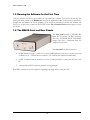
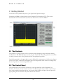
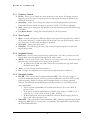
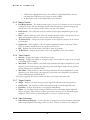
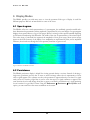
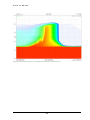
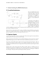
TEST EQUIPMENT PLUS
Signal Hound BB60A
UserManual
TEST EQUIPMENT PLUS
Signal Hound BB60A User Manual
 2013, Test Equipment Plus
35707 NE 86th Ave
La Center, WA
Phone 360.263.5006 • Fax 360.263.5007
Table of Contents
1
PREPARATION ........................................................................................................................................................3
1.1 INITIAL INSPECTION ......................................................................................................................................................... 3
1.2 SOFTWARE INSTALLATION................................................................................................................................................. 3
1.2.1 Software Requirements ....................................................................................................................................... 3
1.3 DRIVER INSTALLATION ..................................................................................................................................................... 4
1.4 CONNECTING YOUR SIGNAL HOUND................................................................................................................................... 4
1.5 RUNNING THE SOFTWARE FOR THE FIRST TIME ..................................................................................................................... 5
1.6 THE BB60A FRONT AND REAR PANELS ............................................................................................................................... 5
2
GETTING STARTED ..................................................................................................................................................6
2.1 THE GRATICULE .............................................................................................................................................................. 6
2.2 THE CONTROL PANEL ...................................................................................................................................................... 6
2.2.1 Frequency Controls .............................................................................................................................................. 7
2.2.2 Span Controls....................................................................................................................................................... 7
2.2.3 Amplitude Controls .............................................................................................................................................. 7
2.2.4 Bandwidth Controls ............................................................................................................................................. 7
2.2.5 Marker Controls ................................................................................................................................................... 8
2.2.6 Trace Controls...................................................................................................................................................... 8
2.2.7 Trigger Controls ................................................................................................................................................... 8
2.2.8 Video Processing.................................................................................................................................................. 8
2.2.9 Acquisition Controls ............................................................................................................................................. 9
2.2.10 Preset ............................................................................................................................................................... 9
2.3 THE MENU .................................................................................................................................................................... 9
2.3.1 File Menu ............................................................................................................................................................. 9
2.3.2 View Menu......................................................................................................................................................... 10
2.3.3 Preferences ........................................................................................................................................................ 10
2.3.4 Presets ............................................................................................................................................................... 10
2.3.5 Settings .............................................................................................................................................................. 10
2.3.6 Spectrum Analysis ............................................................................................................................................. 11
2.3.7 Trace .................................................................................................................................................................. 11
2.3.8 Utilities .............................................................................................................................................................. 11
2.4 THE STATUS BAR .......................................................................................................................................................... 11
2.5 ANNUNCIATOR LIST....................................................................................................................................................... 12
2.6 PLAYBACK TOOLBAR ...................................................................................................................................................... 12
3
MODES OF OPERATION ........................................................................................................................................13
3.1
3.2
3.3
SWEPT ANALYSIS .......................................................................................................................................................... 13
REAL-TIME SPECTRUM ANALYSIS ..................................................................................................................................... 13
ZERO-SPAN ANALYSIS .................................................................................................................................................... 15
3.4
4
TIME-GATE ANALYSIS .................................................................................................................................................... 16
TAKING MEASUREMENTS .....................................................................................................................................17
4.1 MEASURING FREQUENCY AND AMPLITUDE ........................................................................................................................ 17
4.1.1 Using Markers ................................................................................................................................................... 17
4.1.2 Using the Delta Marker ..................................................................................................................................... 17
4.1.3 Measuring Low Level Signals ............................................................................................................................. 17
4.2 SAVING SESSIONS ......................................................................................................................................................... 17
4.3 CAPTURING SIGNALS OF INTEREST .................................................................................................................................... 18
4.4 MEASURING CHANNEL POWER........................................................................................................................................ 18
5
ADDITIONAL FEATURES ........................................................................................................................................19
5.1
5.2
5.3
6
PRINTING .................................................................................................................................................................... 19
SAVING IMAGES ........................................................................................................................................................... 20
IMPORTING PATH LOSS AND LIMIT LINE TABLES .................................................................................................................. 20
DISPLAY MODES ...................................................................................................................................................22
6.1
6.2
7
SPECTROGRAM............................................................................................................................................................. 22
PERSISTENCE................................................................................................................................................................ 22
UNDERSTANDING THE BB60A HARDWARE ...........................................................................................................24
7.1 FRONT END ARCHITECTURE ............................................................................................................................................ 24
7.2 SPURIOUS SIGNALS ....................................................................................................................................................... 24
7.3 RESIDUAL SIGNALS ........................................................................................................................................................ 25
7.4 AMPLITUDE ACCURACY .................................................................................................................................................. 25
7.4.1 Scalloping Loss................................................................................................................................................... 25
7.5 DYNAMIC RANGE.......................................................................................................................................................... 25
8
TROUBLESHOOTING .............................................................................................................................................27
8.1 UNABLE TO FIND OR OPEN THE DEVICE ............................................................................................................................. 27
8.1.1 The Device Light is Green and Still Won’t Connect ............................................................................................ 27
8.1.2 A Power Cycle Does Not Fix the Problem ........................................................................................................... 27
8.2 THE SIGNAL HOUND IS NOT SWEEPING PROPERLY .............................................................................................................. 27
8.2.1 The Sweep is not Updating ................................................................................................................................ 27
8.3 THE DEVICE IS NOT VALID .............................................................................................................................................. 27
9
CALIBRATION AND ADJUSTMENT .........................................................................................................................28
10
SPECIFICATIONS ...................................................................................................................................................29
10.1
10.2
10.3
10.4
10.5
10.6
11
FREQUENCY:............................................................................................................................................................. 29
SWEEP RATE............................................................................................................................................................. 29
AMPLITUDE (RBW ≤100KHZ, IF AUTO-CAL ON) ............................................................................................................. 29
SPECTRAL PURITY ...................................................................................................................................................... 30
TIMING.................................................................................................................................................................... 30
ENVIRONMENTAL ...................................................................................................................................................... 30
WARRANTY AND DISCLAIMER ..............................................................................................................................31
11.1
11.2
11.3
11.4
11.5
11.6
WARRANTY .............................................................................................................................................................. 31
WARRANTY SERVICE .................................................................................................................................................. 31
LIMITATION OF WARRANTY ......................................................................................................................................... 31
EXCLUSIVE REMEDIES ................................................................................................................................................. 31
CERTIFICATION .......................................................................................................................................................... 32
CREDIT NOTICE ......................................................................................................................................................... 32
P R E P A R A T I O N
1 Preparation
The BB60A is a real-time high speed spectrum analyzer communicating with your PC over a USB 3.0
Super Speed link. It has 20 MHz of real-time bandwidth, tunes from 9 kHz to 6 GHz, collects 80 million
samples per second, and streams data to your computer at 140 MB/sec. By adding a high speed hard
drive to your PC or laptop (250 MB/s sustained write speed), the BB60A doubles as an RF recorder,
streaming all 80 million samples per second to disk.
1.1 Initial Inspection
Check your package for shipping damage before opening. Your box should contain a USB 3.0 Ycable, a CD-ROM, and a Signal Hound BB60A.
1.2 Software Installation
Run the setup.exe file from the included CD, and follow on-screen instructions. You must have
administrator privileges to install the software. You may be asked to install the Windows Runtime
Frameworks, as this must be installed for the software to run. During installation, the BB60A device
drivers will also be installed.
It is recommended to install the application folder in the default location.
1.2.1 Software Requirements
Supported Operating Systems

Windows 7 (64-bit)*
3
P R E P A R A T I O N

Windows 8 (64-bit)
Minimum System Requirements



Processor – Intel Desktop quad-core i-Series processors***
RAM – 1 GB for the BB60A software
Native USB 3.0 support
Recommended System Requirements





Windows 7 64-bit
Processor – Intel Desktop quad-core i5 / i7 processors
8 GB RAM
Native USB 3.0 support
OpenGL 3.0 capable graphics processor**
(* Contact Test Equipment Plus for 32-bit operating system drivers.)
(** Certain display features are accelerated with this functionality, but it is not required.)
(*** Our software is highly optimized for Intel CPUs. We recommend them exclusively.)
1.3 Driver Installation
The drivers shipped for the BB60A are for 64-bit operating systems and are placed in the application
folder during installation. The drivers should install automatically during setup. If for some reason the
drivers did not install correctly, you can manually install them by following the instructions below.
To manually install the drivers, navigate to the application folder(where you installed the BB60A
software) and find the InstallDrivers64.exe file. Right click it and Run as administrator. The console
text will tell you if the installation was successful.
You may also manually install the drivers through the Windows device manager. On Windows 7 systems
with the device plugged in, click the Start Menu and Device and Printers. Find the FX3 unknown
USB 3.0 device and right click the icon and select Properties. From there select the Hardware tab and
then Properties. Select the Change Settings button. Hit the Update Drivers button and then Browse
My Computer for drivers. From there navigate to the BB60A application folder and select the folder
name drivers. Hit OK and wait for the drivers to install.
If for some reason the drivers still did not install properly, contact Test Equipment Plus.
1.4 Connecting Your Signal Hound
With the software and BB60A drivers installed, you are ready to connect your device. Plug in both male
USB 3.0 connections into your PCs USB 3.0 ports, and plug the USB 3.0 Micro-B male connection into
the BB60A device. Your PC may take a few seconds recognizing the device and installing any last
drivers. Wait for this process to complete before launching the BB60A software.
4
P R E P A R A T I O N
1.5 Running the Software for the First Time
Once the software and drivers are installed you can launch the software. You can do this through the
desktop shortcut created or the BB60A.exe found in the application folder. If the device is connected a
progress bar will indicate the device preparing. If no device is connected or found, the software will
notify you. At this point, connect the device and use the File->Connect Device menu option to open
the device.
1.6 The BB60A Front and Rear Panels
The front panel includes a 50Ω SMA RF
Input. Do not exceed +20 dBm or damage
may occur. A READY/BUSY LED flashes
orange each time a command from the
computer is processed.
The rear panel has three connectors:
1) 10 MHz Reference input / output. Use a clean 10 MHz reference sine wave or square wave with
>0 dBm level. A +13 dBm sine wave input or 3.3V CMOS clock input is recommended.
2) A USB 3.0 Micro-B female connector. Use the Y-cable provided to connect the device to your
PC.
3) A multi-purpose BNC connector, primarily for trigger input.
Both BNC connectors are also capable of outputting logic high and low using the API.
5
M O D E S
O F
O P E R A T I O N
2 Getting Started
Learn about the basic functions and features of your Signal Hound Spectrum Analyzer.
Launching the BB60A software brings up the Graphical User Interface (GUI). This section
describes the GUI in detail and how you can use the GUI to control the BB60A.
Figure 1 : The BB60A Graphical User Interface
2.1 The Graticule
The graticule is a grid of squares used as a reference when displaying sweeps and when making
measurements. The BB60A displays a ten by ten grid. Inside and around the graticule is text which
can help you make sense of the graticule and the sweeps displaying within.
Outside the graticule in the upper right corner is displayed the temperature of the device in degrees
Celsius. An “Uncal” annunciator will appear above the temperature when the device readings may
be out of spec due to a recent temperature shift.
2.2 The Control Panel
The control panel is the collection of buttons on the right hand side of the Graphical User
Interface. It is home to many common controls. You will recognize many of these controls if you
have used a standard spectrum analyzer. Any control which requires an input value will provide a
pop-up dialog box for numeric entry and relevant unit selection.
6
M O D E S
O F
O P E R A T I O N
2.2.1 Frequency Controls
 Center – allows you to chance the center frequency of the sweep. If a change in center
frequency causes the start or stop frequencies to fall outside the range of operation, the
SPAN will be reduced.
 Start/Stop – allows you to change the sweeps start and stop frequencies respectively.
Frequencies chosen outside the range of operation (9 kHz – 6.5 GHz) are clamped.
 Step – allows you to change the step amount of the up and down arrows. The default step
is 10 MHz
 Up/Down Arrows – change the center frequency by the step amount.
2.2.2 Span Controls
 Span – controls the frequency difference between the start and stop frequencies centered
on the center frequency. A reduced span will be chosen if the new span causes the start or
stop frequencies to fall outside the range of operation.
 Zero Span – Enters Zero-Span mode.
 Full Span – This will change the start, stop, center, and span frequencies to select the
largest span possible.
2.2.3 Amplitude Controls
 Ref Level – sets the power level for the top graticule line. The units you select here will
change which units are displayed throughout the entire system.
 dB/div – sets the scale for the y-axis. It may be set to any positive value. The chosen value
represents the vertical height of one square on the graticule.
o In linear mode, the dB/div control forces the system back into log mode with a
displayed unit of dBm
 Atten – sets the internal electronic attenuator.
 Lin – changes the amplitude scale to linear and the displayed units to millivolts.
2.2.4 Bandwidth Controls
 Res BW – This controls the resolution bandwidth (RBW). For each span a range of
resolution bandwidths may be used. The resolution bandwidth controls the FFT size and
signal processing, similar to selecting the IF bandpass filters on an analog spectrum
analyzer. The selectable bandwidths displayed change whether you want native or nonnative bandwidths.
o Native resolution bandwidths are available from below 1 Hz to 10.1 MHz, in
powers of two.
o Non-Native resolution bandwidths are available from 10 Hz to 10 MHz, in a 1-3
sequence. (e.g. 1 kHz, 3 kHz, 10 kHz, 30 kHz, 100 kHz, … )
o In Real-Time mode, only native bandwidth values are allowed ranging from 2.4
kHz to 631 kHz in powers of two.
 Video BW – This controls the Video Bandwidth (VBW). After the signal has been passed
through the RBW filter, it is converted to an amplitude. This amplitude is then filtered by
the Video Bandwidth filter.
7
M O D E S
O F
O P E R A T I O N
o All Resolution Bandwidth choices are available as Video Bandwidths, with the
constraint that VBW must be less than or equal to RBW.
o In Real-Time mode, Video Bandwidth is not selectable.
2.2.5 Marker Controls
 Left-Right Arrows – The marker controls give you access to 6 markers to use for accurate
readings of sweeps. The left and right arrows scroll through the 6 markers changing the
current active one. All marker controls affect only the active marker.
 Peak Search – This will place the active marker on the highest amplitude signal on the
graticule.
 Delta – places a reference point where the marker currently resides. Once placed you can
make measurements relative to the position of the reference point.
 To Center Freq – changes the center frequency to the frequency location of the current
active marker.
 Update On – When Update is ON, the markers amplitude updates each sweep. When
OFF, the markers amplitude does not update unless moved.
 Off – Disables the current marker, and hides it from the graticule.
 To Ref Level – changes the reference level to the amplitude of the active marker.
2.2.6 Trace Controls
 Normal – Toggles the display of the current sweep.
 Average – Toggles the display of averaged sweeps. The number of sweeps to be averaged
is selectable upon enabling.
 Max Hold – When enabled, a max hold sweep maintains the highest amplitude for each
frequency point. Each sweep, only frequency points with higher amplitudes are updated.
Works simultaneously with Min Hold.
 Min Hold – When enabled, a min hold sweep maintains the lowest amplitude for each
frequency point. Each sweep, only frequency points with lower amplitudes are updated.
Works simultaneously with Max Hold
All sweeps toggled in the Trace Controls are able to be shown at the same time.
2.2.7




Trigger Controls
Single – Request one more sweep from the Signal Hound before becoming inactive.
Continuous – The software continuously requests sweeps from the Signal Hound.
Free Run – In Zero Span mode, a sweep begins immediately.
Video – In Zero Span mode, the Signal Hound waits for a minimum signal amplitude
before sweeping. When clicked, a popup opens where the user sets the minimum signal
amplitude. This is useful for measuring pulses as short as 10 microseconds.
2.2.8 Video Processing
 Video Detector Settings - As the video data is being processed, the minimum, maximum,
and average amplitudes are being stored. You have a choice of which is to be displayed.
8
M O D E S

O F
O P E R A T I O N
Video Processing Units – In the system, unprocessed amplitude data may be represented
as voltage, linear power, or logarithmic power. Select linear power for RMS power
measurements. Logarithmic power is closest to a traditional spectrum analyzer in log scale.
2.2.9 Acquisition Controls
 Sweep Time – In Zero-Span mode, sweep time represents the total amount of time
displayed in the graticule, rounded to the nearest sample. In sweep mode, Sweep Time is
used to modify how long the BB60A dwells on each patch of spectrum. The actual sweep
time may be significantly different from the time requested, depending on RBW, VBW, and
span settings, as well as hardware limitations.
 Spur Rejection – When spur rejection is on additional signal processing is enabled
attempting to remove spurious signals which are the result of mixing products. Spur
rejection roughly doubles sweep time and is great for cleaning up a steady signal, but should
not be used for pulsed RF. Spur rejection is not available in real-time mode.
 IF Self Cal – The BB60A device is temperature sensitive. The software updates these
temperature calibrations when it sees a 2 °C change. To manually recalibrate the device for
temperature changes at any time, use this button.
 Gain – Gain is used to control the input RF level. With this control you can have the gain
determined automatically or choose 4 levels of gain. Higher gains increase RF levels. When
gain is set to automatic, a best gain is chosen based on reference level. Manual gain settings
may cause the signal to clip well below the reference level, and should be used by
experienced BB60A users only.
2.2.10 Preset
 Preset – Restores the software and hardware to its initial power-on state by performing a
device master reset.
2.3 The Menu
2.3.1








File Menu
Recall – Begin playing a saved session. (See Getting Started: Playback Toolbar)
Save – Begin recording a new session. (See Getting Started: Playback Toolbar)
Save as .bmp – Save the current graticule view as a bitmap image.
Print – Print the current graticule view. The resulting print will not include the control
panel or the menu/toolbars.
Print Preview – Shows you what will be printed using the print menu option.
Connect Device – If no device is connected, this option will attempt to connect to the
first BB60A device found.
Disconnect Device – This option disconnects the currently connected BB60A device.
This option combined with “Connect Device” is useful for cycling a devices power or
swapping devices without closing the Signal Hound software.
Export→Trace CSV – Saves the current visible trace as a CSV file.
9
M O D E S
O F
O P E R A T I O N

Import→Path Loss Table – This menu option allows you to introduce path loss
corrections for the incoming traces. See Additional Features : Importing Path Loss and
Limit Line Tables for more information.
 Import→Limit Line Table – Import a set of limit lines which then the incoming trace is
tested against. Limit lines are two lines across the span which define an acceptable region
for a trace. You can specify a maximum limit or a maximum and minimum set. See
Additional Features : Importing Path Loss and Limit Line Tables for more
information.
2.3.2 View Menu
 Colors – The colors menu provides the ability to change the graticule color scheme. Two
color schemes are available, default(white on black), and printer friendly(black on white). If
these are not to your liking, you can create a custom color scheme and tell the software to
use your scheme for future application invocations.
 Title – Enable or disable a custom title. The title appears above the graticule and is included in
screen captures via printing as well as session recordings.
2.3.3 Preferences
 Window Type – This menu option allows you to select between four windowing functions
used in the signal processing. To have access to all four windowing function, you must be
in sweep/time-gate mode and using native RBWs. In all other cases, the Nuttall window
function will be used.
 Spectrogram – Preferences related to the two and three dimensional spectrogram displays.
o Color Blind – Change between a color spectrum and black and white spectrum.
 Persistence – Preferences related to the persistence display. (See Displays: Persistence
for more information regarding persistence)
o Decay Rate – The decay rate determines how long a trace will impact the
persistence display. Lower decay rates result in traces fading away slower, while
higher decay rates result in traces fading quickly.
 Trace Line Width – Change the width of the trace lines. Affects all non-persistence and
non-spectrogram traces.
 Calibration – Change whether temperature calibrations are made automatically during
operation.
2.3.4 Presets
 Save As – Save the current device settings for later use.
 Load – Load a previously saved preset.
2.3.5 Settings
 Reference Level Offset – Adjust the displayed amplitude to compensate for an attenuator,
probe, or preamplifier.
 Downconverter Offset – Apply a fixed frequency offset to the display and marker readout
to compensate for your downconverter LO.
10
M O D E S






O F
O P E R A T I O N
Sweep Time – Adjust how long the device acquires data before processing. Processing
time and memory usage increases as sweep time increases. Applies to sweep and zero-span
modes only.
Real-Time Update Interval – Change how long data is masked together in real-time
mode before returning a trace.
Zero-Span Analysis – Brings up a dialog allowing you to change zero-span settings.
o Trigger Type – Choose between no trigger, video trigger, or an external trigger.
o Y Axis – Change the demodulation type between AM and FM.
o Trigger Height – Change the value on which a trigger becomes active.
o Trigger Time – The maximum amount of time to look for a trigger for each
sweep. If no trigger is found, the last possible section of the sweep is returned.
o Trigger Edge – Determined whether to trigger on a rising or falling edge.
Time-Gate Analysis – Brings up a dialog allowing you to change time-gate settings.
o Gate Length – How much spectrum to analyze.
o Capture Length – Amount of time to look for a trigger/gate.
o Gate Delay – Amount of time between the trigger and the beginning of the gate.
o Trigger Edge Type – Determine whether to trigger on a rising or falling edge.
RF Bypass – N/A
Reference – Change the source of the BB60A’s reference oscillator. You can choose to use
the internal reference or an attached 10MHz reference on the appropriate BNC port.
2.3.6 Spectrum Analysis
 Idle – Cause the device to enter an idle mode. No trace is displayed in this mode. Playback
is possible in idle mode.
 Swept Analysis – Enter standard swept analysis.
 Real-Time Analysis – Enter real-time mode.
 Zero-Span – Enter zero-span mode.
 Time-Gate Analysis – Enter time-gate analysis.
2.3.7






Trace
Copy Trace – Copy the currently displayed trace to one of two available copies.
Show Trace – Toggle the display of the two trace copies.
Disable – Disable the limit lines or path loss tables.
Persistence – Enable/Disable/Clear the persistence trace.
Spectrogram – Enable/Disable spectrogram display.
Signal Tracking – Enable/Disable signal tracking.
2.3.8 Utilities
 Channel Power – Enable/Disable the channel power utility.
2.4 The Status Bar
The status bar runs across the bottom of the BB60A application. When the mouse enters the graticule
the status bar displays the frequency/time value for the x-axis and the amplitude/frequency value for the
11
M O D E S
O F
O P E R A T I O N
y-axis. The status bar readings should not be used for precise measurements, but is great for quick
estimations.
2.5 Annunciator List
On the upper right hand corner of the graticule, you will find a list of annunciators. Annunciators are
provided as warnings and indicators providing useful information to the operator. Below is a list of all
annunciators and their meanings.
Temperature – The device temperature is always displayed in °C. This is the device’s internal
temperature.
ADC – This indicator appears when hard compression is present on the displayed sweep. This occurs
when the input RF signal reaches the maximum possible digital level. To fix this, you can increase the
reference level, increase attenuation, or lower gain.
TEMP – This indicator appears when the device has deviated more than 2 °C since its last temperature
calibration. The software will automatically calibrate under specific circumstances, the device is not in
real-time mode and the user has selected the SettingsCalibrationAuto menu option (enabled by
default). Manually recalibrate the device by pressing the Self-Cal IF control panel button.
LOW V – This indicator appears when the device is not receiving enough voltage from the USB 3.0
connection. The voltage value appears when this annunciator is present. The device requires 4.4V. If this
annunciator appears, it may indicate other problems. Contact Test Equipment Plus if you are unable to
determine the source of this problem.
UNCAL – This indicator appears whenever any warning indicator is active to notify the user that the
device may not be meeting published specifications.
2.6 Playback Toolbar
The playback toolbar controls the recording and playback of sessions. Sessions are a collection of saved
sweeps at one device setting.
1. Record – Begins recording a session
2. Stop Recording – Stops recording an active session.
3. Play/Continue – Begin playing a saved session or continue a paused session.
4. Stop – Stop playing the current session.
5. Pause – Pause the current session.
6. Rewind – Rewinds then pauses the session.
12
M O D E S
O F
O P E R A T I O N
7. Step Back – Shows the previous trace in the session and pauses.
8. Step Forward – Shows the next trace in the session and pauses.
9. Timer – Specify in milliseconds the amount of time to wait before displaying the next trace in
the session, up to 2000ms.
3 Modes of Operation
The BB60A is a hybrid superheterodyne-FFT spectrum analyzer. The BB60A is a combination of swepttuned and FFT based analyzers. The BB60A uses a oscillator and band-pass filter to down-convert a
portion of the input spectrum into an intermediate frequency (IF). The intermediate frequency is then
sent from the device to the host PC where it undergoes FFT spectrum analysis transforming the input IF
into a frequency spectrum.
The IF resulting from the down-conversion contains 20 MHz of usable bandwidth.
The BB60A is also a real-time spectrum analyzer. This means the device is capable of continuously
streaming a 20 MHz IF frequency with no time gaps. Having no time gaps is critical for measurements
and tests requiring high probability of intercept (POI). See the section below Real-Time Spectrum
Analysis for a more in-depth discussion of the BB60A capabilities.
The BB60A offers multiple modes of operation. Most of these are exposed in the software and others
can be exposed through our C-based API. We will only cover those in our software here.
3.1 Swept Analysis
This mode of operation is the mode which is commonly associated with spectrum analyzers. Through
the software you will configure the device and request the device perform a single sweep across your
desired span. Since the BB60A has a max bandwidth of 20MHz, spans larger than 20MHz are the result
of acquiring multiple 20MHz patches and concatenating the results of the FFT processing on each of
these IFs.
The processing performed on each 20MHz patch is determined by the settings provided. Each time a
trace is returned, the device waits until the next trace request. For you, the software user, you can choose
to continuously retrieve traces or manually request them one at a time with the Single and Continuous
buttons found on the Trace Controls.
3.2 Real-Time Spectrum Analysis
One of the issues with the standard sweep mode is the “blind time” between each trace. Blind time
refers to the time between spectrum sampling. During this time, we are processing the last capture, or
viewing the data. During this time it is possible to miss an event. The picture below shows a missed
event in green.
13
M O D E S
O F
O P E R A T I O N
In this image we see an event missed due to the blind time between spectrum sampling. With Real-Time
spectrum analysis we can prevent this and capture ALL possible events.
As discussed above, the BB60A is capable of streaming a 20MHz bandwidth with no time gaps. If we
limit our spans to 20MHz we can now process every spectrum sample for our resulting trace. The
BB60A performs overlapping FFTs at an overlapping rate of 75%, covering each point of data with 4
FFTs. We take the resulting FFTs and min/max them into a final returned trace. The number of FFT
results merged depends on Real-Time Sweep Time and the RBW.
14
M O D E S
O F
O P E R A T I O N
3.3 Zero-Span Analysis
Zero span allows you to view a signal in time domain.
The y-axis can be either amplitude or frequency, and the
x-axis is always time. Before entering zero-span analysis
mode, modify your Zero Span Settings from the Settings
menu.
Zero-span allows you to specify a video trigger, external
trigger, or no trigger. Video triggers allow you to begin the
sweep only after a signal exceeds the amplitude specified
in “trigger height.” This is useful when you need to
analyze a periodic transmission.
If your transmitter has a trigger output, you can route this
to the BB60 trigger in. Select “external trigger” to cause
the zero-span sweep to begin after this hardware trigger. You can trigger on the rising edge or falling
edge of a signal. A 3.3V CMOS trigger with a 50 ohm output impedance is ideal, but 5V logic with a 50
ohm output impedance is acceptable. Higher or lower output impedance may work with a short BNC
cable, but longer cables may cause issues with reflection.
The sweep typically begins approximately 200 microseconds before the trigger event, allowing you to
view a sliver of what was happening before the trigger. Do not use this zero span mode for precision
timing applications. Please see the API manual for functions supporting precision time stamps.
The BB60 will wait up to a maximum of “Max Trigger Time” looking for a trigger. If none is found, it
will automatically trigger at the end of the allotted time.
If your trigger output is sensitive to loading, start zero span mode before connecting your trigger, to
ensure the BB60 trigger port is configured as an input.
15
M O D E S
O F
O P E R A T I O N
3.4 Time-Gate Analysis
Time Gate analysis allows you to specify a time
window in which the BB60A will measure the
spectrum. With the use of an external input trigger
you can define very precise time restrictions for
spectrum analysis. Time Gate analysis is useful for
synchronizing your transmitter duty cycle with your
BB60 spectrum analyzer capture window, for
example when you need to analyze a time-division
multiplexed transmitter.
The above picture shows the spectrum of a pulse modulated signal without time-gate analysis. The
picture, below, shows the same signal, time gated for when the transmitter is on.
In Time-Gate analysis the “gate” is referred to as the
time period of interest. Ideally with an external
trigger triggering before the gate of interest we can
specify a few numbers to acquire our gate. We need
to know the length of the gate and the amount of
time after a trigger in which the gate occurs. The gate
length must be large enough to perform the required
FFTs based on your RBW and VBW. The software
will notify you if a longer gate or higher RBW /
VBW are required.
16
A D D I T I O N A L
F E A T U R E S
4 Taking Measurements
This section helps you learn how to measure, analyze, and record signals using the BB60A, utilizing builtin features such as markers, record/playback, and channel power.
4.1 Measuring Frequency and Amplitude
4.1.1 Using Markers
There BB60A software has several tools for identifying a signal’s frequency and amplitude. The easiest to
use is the marker. There are 9 markers available, each with its own reference.
To active and place a marker you can left click inside the graticule or press the Peak Search button on
the marker controls to place the marker on the current trace peak and activate it simulatenously. Once a
marker is active the frequency and amplitude readout of the marker is located below the graticule. The
marker’s accuracy is dependent on the span and RBW. Narrower spans and RBWs have higher marker
accuracy. The amplitude accuracy is NOT dependent on the vertical dB/div, since the I/Q data is linear
in voltage and has much higher resolution than is displayed. The marker may be re-placed at any time by
clicking the graticule or by using the left and right arrows to shift the marker one sample point to the left
or right.
4.1.2 Using the Delta Marker
To measure differences or changes in frequency and/or amplitude you can use the delta markers. To
use the delta markers you must first create a reference point. With a marker active click the Delta control
panel button. This places a reference location on the graticule. Now you can move the marker elsewhere
on the graticule and the marker readings below the graticule will report the difference between the
marker and the reference.
4.1.3 Measuring Low Level Signals
To measure low-level signals, there are a few tricks to getting accurate readings. First of all, set the
internal electronic attenuator to 0 dB (click the atten button). Then, set your reference level to -50
dBm or lower. This internally selects the highest sensitivity settings. Using an external timebase and
narrow span (1 KHz or less) should give you better results. Video averaging may be required for a
stable amplitude reading.
4.2 Saving Sessions
The playback toolbar allows you to record and replay a continuous session up to 1GB. The length of the
session will be dependent on the average sweep speed of the session and trace length. Sessions files have
the extension “.b6p” and are named based on the current time and date. This naming scheme ensures no
files are overwritten and relieves you of determining file names when you really want to cature a signal
NOW. Pressing record on the playback tool bar causes the software to immediately begin recording. All
playback files are saved in your “My Documents” folder.
When replaying all functionality of the software remains. You can place markers, activate
min/max/average traces as well as view the recording using persistence and spectrogram views. In
addition the playback toolbar allows you to pause, step, and rewind your way through a saved session.
17
A D D I T I O N A L
F E A T U R E S
Tip: The title is also recorded and shown
during playback. Use a title to describe the
session!
4.3 Capturing Signals of Interest
CSV files can be created of traces using the File menu option. CSV files are useful for performing further
signal analysis or plotting outside the Signal Hound application. When exporting a trace into a CSV file,
the currently shown trace is exported. Because of this it may be difficult to obtain a CSV file of a signal
of interest. For example, an intermittent signal which appears sporadically may be difficult to capture, or
some modes such as Real-Time signal analysis are prohibited from saving CSV files.
One way to export a desired signal is to record the spectrum using the playback toolbar. If you are able
to capture your signal in a playback session, you can playback the session and pause on your trace of
choice. While paused you can export the trace.
Min and Max hold traces are another way to capture intermittent hard to view signals. Min and max hold
keep track of the minimum and maximum values over a period of time storing them in a separate
viewable trace. When min/max hold is active, markers automatically clamp to that trace.
4.4 Measuring Channel Power
The Utilities menu includes a Channel Power utility. When selected, a popup will appear requesting a
channel bandwidth and channel spacing. Channel bandwidth is width in Hz of the band whose power
you wish to measure. Channel spacing refers to the center-to-center frequency difference. Between
channels, there is typically (but not always) a small guard band whose power is ignored.
For example, the image below shows a channel bandwidth of 180 kHz and spacing of 200 kHz. The
image shows the FM station 101.1 in the center channel. Each channel will be integrated and the
resulting power is display at the top of the channel.
The adjacent channels also show the channel power as well as the difference in power between the
center channel and itself. In the example below the difference might be used to determine if any power is
“leaking” into an adjacent FM band.
18
A D D I T I O N A L
F E A T U R E S
For best results, set your video processing to AVERAGE, POWER, and turn spur reject off. A native
bandwidth must be selected for accurate power measurements. The software will set most of this up for
you automatically.
5 Additional Features
The BB60A software has a number of useful utilities. They are described here.
5.1 Printing
Using the File – Print menu you can print exactly what is shown on the graticule. Be careful, if the
software is still updating traces, you may not print the trace you wanted. Use the print preview option to
see exactly what you will be printing.
Tip: The active color scheme is used for
printing as well. Under the View –
Colors menu, we provide a simple printer
friendly color scheme to help you save
ink!
19
A D D I T I O N A L
F E A T U R E S
5.2 Saving Images
Using the File- Save as .bmp menu option you can save the current graticule view as a bitmap image.
The resulting resolution of the image is the exact resolution of your graticule when you choose to save.
To obtain the highest resolution image, maximize the software and slide the control panel out of the
way. The active color scheme is used in the resulting image.
5.3 Importing Path Loss and Limit Line Tables
Using the File->Import menu options you can import path loss and limit line tables from simple .csv
files. CSV stands for Comma Separated Value. The format for a typical file might look like this..
23.56, 32
123.45, 512
…
Two or more values separated by a comma, each line ending with a carriage return. These files can be
created with a simple text editor or spreadsheet program like Microsoft Excel.
For path loss tables we use a CSV file with two values per line. The first value on each line is a frequency
value in MHz and the second value is a dBm offset. The frequency values must be in increasing order.
The path loss corrections are linearly interpolated between these data points and are flat entering and
leaving the span with the amplitude of the flat corrections being the first and last data point respectively.
Here is an example of a path loss CSV file built in a spreadsheet program.
732
738
0
2
And here is the resulting path loss corrections applied to incoming traces for a 10MHz span
centered at 735 MHz.
20
A D D I T I O N A L
F E A T U R E S
We can see the linear interpolation between the two points and flat lines off the sides.
The format for limit lines is very similar. Each line with contain two or three values. If you only
want a max limit line, each line of the CSV will contain two values, if you want max and minimum
limit lines, each line will contain three values. The first value will be a frequency in MHz, followed
by the (optional) minimum amplitude in dBm, and the maximum amplitude in dBm.
The limit lines are drawn on the graticule and every trace is tested against them. Indicator text will
appear in the center of the screen denoting whether the trace currently shown passes or fails the
limit line test.
21
D I S P L A Y
M O D E S
6 Display Modes
The BB60A provides you with many ways to view the spectrum. Each type of display is useful for
different purposes. Below is an introduction to some of the views.
6.1 Spectrogram
The BB60A offers two visual representations of a spectrogram, the traditional spectral waterfall and a
three dimensional representation where amplitude is represented by color and height. Our spectrogram
displays show spectral history of up to 128 sweeps. Below is an image of the spectral waterfall displaying
an FM station broadcasting with HD radio. The width of the view is representative of the selected span.
The colors along a horizontal line represent the amplitude of that given sweep. More recent sweeps
appear at the front (bottom) of the display. Low amplitudes are represented by blue, and as amplitude
increases, the color moves through the color spectrum, from blue to green to red.
Figure 2 : FM Station with HD Radio side bands
6.2 Persistence
The BB60A persistence display is helpful for viewing spectral density over time. Instead of showing a
single trace, persistence uses the last ‘n’ traces to create an image where color is representative of how
often a signal appears. The software uses the color spectrum to represent density over time. If a signal
rarely occurs in a location, a light blue is used to color the trace. If a signal continues to appear in the
same location the color will change from blue to green to red. Red is an indication of a signal persisting
in one location for a good deal of time. Using the Preferences  Persistence  Decay Rate menu
option, you can control how fast traces accumulate on the screen.
22
D I S P L A Y
M O D E S
Figure 3: Persistence showing the signal from a poorly shielded commercial microwave oven in Real-Time mode.
23
U N D E R S T A N D I N G
T H E
B B 6 0 A
H A R D W A R E
7 Understanding the BB60A Hardware
7.1 Front End Architecture
The AC-coupled RF input is first
attenuated. It then passes through
a band select filter to reject the
image and out-of-band responses,
after which it is amplified or
attenuated before mixing (a gain
setting of 1 or less attenuates the
RF).
At the mixer, a local oscillator is
injected high-side to produce the
intermediate frequency (IF). This
IF is either ~2.35 GHz, or ~1.27
GHz, depending on band. The IF
passes through a SAW filter with
approx. 60 MHz of bandwidth,
and is then amplified or attenuated (a gain of 0 attenuates the IF). The SAW filters were selected to have
good rejection 280 MHz from center.
Inside the IF-to-bits subassembly, the IF is mixed to 140 MHz (the image 280 MHz away having been
filtered out in the previous step), filtered to a 20 MHz bandwidth, then digitized at 80 MSPS. Additional
gain may be applied in the IF-to-bits subassembly when gain is set to 3.
7.2 Spurious Signals
A spurious signal appears as a function of an input signal. These include signals from intermodulation,
image responses, local oscillator spurs, and ADC aliasing.
Spurious signals from intermodulation can be controlled by limiting the amount of power into a mixer or
amplifier. Decreasing the power by 10 dB will often reduce intermodulation products by 20 or 30 dB.
One source of image-related spurious signals comes from the image from the first mixer. These are
usually far from the signal of interest and very low in amplitude, especially below 2 GHz, but may be
something like -40 dBc in small areas of the upper bands. These spurs will be rejected using the software
“spur reject.”
Another source of spurs occurs when LO1 exceeds 4.4 GHz. The LO is doubled in this case,
introducing spurs from the LO subharmonic. This is especially noticeable when you are sweeping across
5.7 GHz, as a signal injected at 4 GHz will create a false spur which may be something like -28 dBc from
the actual signal. These spurs will be rejected using the software “spur reject.”
24
U N D E R S T A N D I N G
T H E
B B 6 0 A
H A R D W A R E
Other spurs may occur 280 MHz below the actual signal, from the IF filter rejection. These are usually
quite low.
Finally, some spurs are introduced during the final mixing and digitizing. Anything not rejected by the
final 140 MHz may be aliased into the data, specifically signals 30-50 MHz above and below the desired
signal. These are typically about –50 dBc, but may be higher near gain compression. These will generally
be rejected by using the software “spur reject,” but there are some exceptions, especially even multiples
of 10 MHz.
For spans below 500 kHz and some streaming and zero-span modes, additional spurs from the
fractional-N local oscillator may be observed. These will usually be below -50 dBc, and will generally be
rejected by using the software “spur reject.”
7.3 Residual Signals
A residual signal appears even when there is no signal input. The BB60A has noticeable residual signals
at multiples of its 10 MHz timebase. These are guaranteed to be below -90 dBm for a reference level of
-50 dBm, attenuator 0 dB (for advanced users, 0 dB atten, gain of 2 or 3), but will typically be well below
this level. For higher reference levels or lower gain, these may be higher. If these residual signals interfere
with your signal measurements, an external RF amplifier may be needed.
7.4 Amplitude Accuracy
Some of the filters are temperature-sensitive. We have included an automatic self-calibration when a
significant temperature change is observed. If this is turned off, a temperature change may introduce
amplitude ripple in the passband, increasing measurement error by a dB or more in some cases. Because
of this, bypassing the automatic self-cal is not recommended when amplitude accuracy is important.
7.4.1 Scalloping Loss
The “native” bandwidths used in the BB60A come directly from the windowed FFT results. When a
signal falls between two “bins,” the energy is split between adjacent bins such that the reported “peak”
amplitude may be lower by as much as 0.8 dB. If frequency resolution and processing speed are more
important than absolute amplitude, use native bandwidths.
To get an accurate power reading using “Marker peak”, non-native bandwidths are recommended. They
integrate the power across several adjacent bins, eliminating scalloping loss.
The “channel power” utility, which integrates the power across any channel bandwidth you specify, also
eliminates this scalloping loss.
7.5 Dynamic Range
The BB60A software will automatically select internal gain settings for best dynamic range when the
input signal is equal to reference level, given your selected attenuator setting. You may notice, as you
increase reference level, the noise floor suddenly jump up. This is from a step in the internal gain setting.
25
U N D E R S T A N D I N G
T H E
B B 6 0 A
H A R D W A R E
These gain steps may be 20 dB or more in some cases. Because of this, increasing or decreasing your
attenuator setting by 10 dB may allow the software to select a more optimal gain setting, significantly
improving your dynamic range.
For large spans crossing multiple bands, you may notice a step in the noise floor. This is due to different
sensitivities and gain settings for each band. Changing your reference level or attenuator setting by 10 dB
may reduce this step if desired.
Advanced API users gathering uncorrected data with the BB60A have an additional tool for optimizing
dynamic range, as the uncorrected data is referenced to full scale ADC readings. In most gain settings,
the best compromise between dynamic range and spurious is achieved when the signal is reading -10 to 20 dB Full Scale (dBFS). Simply choose an appropriate gain and fine tune your attenuator setting to
optimize for your needs.
26
T R O U B L E S H O O T I N G
8 Troubleshooting
If you experience a problem with your Signal Hound, please try these troubleshooting techniques before
contacting us.
8.1 Unable to Find or Open the Device
Ensure the device is plugged in and the green light is on. If it is not, unplug then plug in the device. Once
the green light turns on, use the File menu to try to connect the device again.
8.1.1 The Device Light is Green and Still Won’t Connect
This is often the case when the device is plugged in when a PC has been turned on. We recommend
leaving the device unplugged when you turn off your PC. If this is the case, a power cycle will solve this
issue.
8.1.2 A Power Cycle Does Not Fix the Problem
If a power cycle still does not allow you to connect the device, it is possible the device drivers were not
successfully installed. See the Driver Installation section for information about the BB60A drivers.
8.2 The Signal Hound is Not Sweeping Properly
If the sweeps shown are not what you expect there are a number of things you can try.
1) In the preset menu, Load->Factory Settings will return the application to default start up
settings. This might be useful if you managed to change a setting and can’t undo it.
2) Restarting the application is a quick way to reset any unknown settings or state.
3) The green Preset button located on the control panel performs a hard reset for the device and
the software settings. In rare instances, communication between the application and device can
become corrupted. The preset button should be used any time the device enters an undesirable
state.
8.2.1 The Sweep is not Updating
When the BB60A is unplugged from the USB 3.0 port while operating, the software may continue
looping through the last sweep in some modes. To rectify this, plug the BB60 back in and click Preset.
8.3 The Device is Not Valid
In the event the device ceases to operate or becomes corrupted, the application might tell you the device
does not appear to be valid. Before contacting us, attempt to power cycle the device and restart your
computer to ensure nothing else is causing this issue. If the issue persists, please contact us.
27
C A L I B R A T I O N
A N D
A D J U S T M E N T
9 Calibration and Adjustment
Contact Test Equipment Plus for more information regarding calibration software and required
equipment.
28
S P E C I F I C A T I O N S
10 Specifications
10.1 Frequency:
Range: 9 kHz to 6.0 GHz
Streaming IF or I/Q data: 20 MHz real-time analysis BW
Resolution Bandwidths (RBW): 10 Hz to 10 MHz
Internal Timebase Accuracy: ±1ppm per year
10.2 Sweep Rate
Sweep Speed (RBW ≥ 9.86 kHz):
(“Spur Reject” off) ≥24 GHz/sec
(“Spur Reject” on) ≥12 GHz/sec
Note: Non-native bandwidths or lower VBWs will result in slower sweep speeds. Sweep speed
does not count sweep setup time (typically <20 ms)
10.3 Amplitude (RBW ≤100kHz, IF auto-cal on)
Range: +10 dBm to Displayed Average Noise Level (DANL)
Absolute Accuracy*: ±2.0 dB
Displayed Average Noise Level (dBm/Hz), reference level -60 dBm, atten 0 dB:
9 kHz to 100 kHz
-123
100 kHz to 200 kHz
-132
200 kHz to 300 kHz
-142
300 kHz to 6 GHz
-152
Residual Responses (includes 10 MHz timebase multiples):
(≤ -50 dBm Ref Level, 0 dB Atten) –90 dBm
LO Leakage: ≤ -65 dBm
Please note: native bandwidths have additional “scalloping loss” of up to 0.8 dB. Use non-native (1/3/10)
bandwidths or the channel power tool for critical amplitude measurements.
*Device must be plugged in for at least 5 minutes to guarantee amplitude accuracy.
29
S P E C I F I C A T I O N S
10.4 Spectral Purity
Spurious & Image Rejection (–20 dBFS into ADC, 0dB attn., max gain) typical:
SW Spur Reject 9 kHz to 1.5 GHz
Off
-39 dBc
On
-39 dBc
Phase noise at 1 GHz:
Frequency Offset
100 Hz
1 kHz
10 kHz
100 kHz
1 MHz
1.5 GHz to 5.0 GHz
-37 dBc
-46 dBc
5.0 GHz to 6.0 GHz
-22 dBc
-48 dBc
dBc/Hz
-70
-78
-84
-96
-116
LO Leakage: ≤ –65 dBm out the RF input connector
10.5 Timing
External Trigger: ±50 nS (4 samples)
GPS Synchronization: 1-PPS GPS precision time stamping
Accuracy: ±50 nS (4 samples) plus GPS error
10.6 Environmental
Operating Temperature: 32°F to 122°F (0°C to +50°C) without derating specifications
Typical internal temperature is 15°C above ambient. Internal temperature is not to exceed 70°C
while operating.
Size and Weight:
7.63” x 3.19” x 1.19” (194mm x 81mm x 30mm)
Net, 0.69 lb. (0.31 kg)
30
W A R R A N T Y
A N D
D I S C L A I M E R
11 Warranty and Disclaimer
©Copyright 2013
Test Equipment Plus
All rights reserved
Reproduction, adaptation, or translation without prior written permission is prohibited,
except as allowed under the copyright laws.
11.1 Warranty
The information contained in this manual is subject to change without notice. Test
Equipment Plus makes no warranty of any kind with regard to this material, including,
but not limited to, the implied warranties or merchantability and fitness for a particular
purpose.
Test Equipment Plus shall not be liable for errors contained herein or for incidental or
consequential damages in connection with the furnishing, performance, or use of this
material. This Test Equipment Plus product has a warranty against defects in material
and workmanship for a period of one year from date of shipment. During the
warranty period, Test Equipment Plus will, at its option, either repair or replace
products that prove to be defective.
11.2 Warranty Service
For warranty service or repair, this product must be returned to Test Equipment Plus.
The Buyer shall pay shipping charges to Test Equipment Plus and Test Equipment
Plus shall pay UPS Ground, or equivalent, shipping charges to return the product to
the Buyer. However, the Buyer shall pay all shipping charges, duties, and taxes, to and
from Test Equipment Plus, for products returned from another country.
11.3 Limitation of Warranty
The foregoing warranty shall not apply to defects resulting from improper use by the
Buyer, Buyer-supplied software or interfacing, unauthorized modification or misuse,
operation outside of the environmental specifications for the product. No other
warranty is expressed or implied. Test Equipment Plus specifically disclaims the
implied warranties or merchantability and fitness for a particular purpose.
11.4 Exclusive Remedies
The remedies provided herein are the Buyer’s sole and exclusive remedies. Test
Equipment Plus shall not be liable for any direct, indirect, special, incidental, or
consequential damages, whether based on contract, tort, or any other legal theory.
31
W A R R A N T Y
A N D
D I S C L A I M E R
11.5 Certification
Test Equipment Plus certifies that, at the time of shipment, this product conformed to
its published specifications.
11.6 Credit Notice
Windows is a registered trademark of Microsoft Corporation in the United States and other countries.
Intel® and Core™ are trademarks or registered trademarks of the Intel Corp. in the USA and/or other countries.
32