1
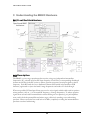
SIGNAL HOUND BB60C / BB60A UserManual SIGNAL HOUND BB60C / BB60A User Manual Version 2 2014, Signal Hound 35707 NE 86th Ave La Center, WA Phone 360.263.5006 • Fax 360.263.5007 Table of Contents 1 OVERVIEW .............................................................................................................................................................4 1.1 2 WHAT’S NEW ................................................................................................................................................................ 4 PREPARATION ........................................................................................................................................................4 2.1 INITIAL INSPECTION ......................................................................................................................................................... 4 2.2 SOFTWARE INSTALLATION................................................................................................................................................. 5 2.2.1 Software Requirements ....................................................................................................................................... 5 2.3 DRIVER INSTALLATION ..................................................................................................................................................... 5 2.4 CONNECTING YOUR SIGNAL HOUND................................................................................................................................... 6 2.5 RUNNING THE SOFTWARE FOR THE FIRST TIME ..................................................................................................................... 6 2.6 THE BB60 FRONT AND REAR PANELS ................................................................................................................................. 6 3 GETTING STARTED ..................................................................................................................................................8 3.1 THE GRATICULE .............................................................................................................................................................. 8 3.2 THE CONTROL PANELS ..................................................................................................................................................... 8 3.2.1 Frequency Controls .............................................................................................................................................. 9 3.2.2 Amplitude Controls .............................................................................................................................................. 9 3.2.3 Bandwidth Controls ............................................................................................................................................. 9 3.2.4 Acquisition Controls ........................................................................................................................................... 10 3.2.5 Trace Controls.................................................................................................................................................... 10 3.2.6 Marker Controls ................................................................................................................................................. 11 3.2.7 Offsets ............................................................................................................................................................... 12 3.2.8 Channel Power................................................................................................................................................... 12 3.3 SWEEP TOOLBAR .......................................................................................................................................................... 12 3.4 THE MENU .................................................................................................................................................................. 12 3.4.1 File Menu ........................................................................................................................................................... 12 3.4.2 Edit Menu .......................................................................................................................................................... 13 3.4.3 Presets ............................................................................................................................................................... 13 3.4.4 Settings .............................................................................................................................................................. 13 3.4.5 Spectrum Analysis ............................................................................................................................................. 14 3.4.6 Trace .................................................................................................................................................................. 14 3.4.7 Utilities .............................................................................................................................................................. 14 3.5 PREFERENCES............................................................................................................................................................... 14 3.6 THE STATUS BAR .......................................................................................................................................................... 15 3.7 ANNUNCIATOR LIST....................................................................................................................................................... 15 3.8 PLAYBACK TOOLBAR ...................................................................................................................................................... 16 4 MODES OF OPERATION ........................................................................................................................................16 4.1 SWEPT ANALYSIS .......................................................................................................................................................... 16 REAL-TIME SPECTRUM ANALYSIS ..................................................................................................................................... 17 4.2 5 TAKING MEASUREMENTS .....................................................................................................................................18 5.1 MEASURING FREQUENCY AND AMPLITUDE ........................................................................................................................ 18 5.1.1 Using Markers ................................................................................................................................................... 18 5.1.2 Using the Delta Marker ..................................................................................................................................... 18 5.1.3 Measuring Low Level Signals ............................................................................................................................. 18 5.2 SAVING SESSIONS ......................................................................................................................................................... 18 5.3 CAPTURING SIGNALS OF INTEREST .................................................................................................................................... 19 5.4 MEASURING CHANNEL POWER........................................................................................................................................ 19 6 ADDITIONAL FEATURES ........................................................................................................................................20 6.1 6.2 6.3 6.4 7 PRINTING .................................................................................................................................................................... 20 SAVING IMAGES ........................................................................................................................................................... 21 IMPORTING PATH LOSS AND LIMIT LINE TABLES .................................................................................................................. 21 AUDIO PLAYER ............................................................................................................................................................. 23 DISPLAY MODES ...................................................................................................................................................23 7.1 7.2 8 SPECTROGRAM............................................................................................................................................................. 23 PERSISTENCE................................................................................................................................................................ 24 UNDERSTANDING THE BB60A HARDWARE ...........................................................................................................26 8.1 FRONT END ARCHITECTURE ............................................................................................................................................ 26 8.2 SPURIOUS SIGNALS ....................................................................................................................................................... 26 8.3 RESIDUAL SIGNALS ........................................................................................................................................................ 27 8.4 AMPLITUDE ACCURACY .................................................................................................................................................. 27 8.4.1 Scalloping Loss................................................................................................................................................... 27 8.5 DYNAMIC RANGE.......................................................................................................................................................... 27 9 UNDERSTANDING THE BB60C HARDWARE ...........................................................................................................29 9.1 9.2 10 FRONT END ARCHITECTURE ............................................................................................................................................ 29 DESCRIPTION ............................................................................................................................................................... 29 TROUBLESHOOTING .............................................................................................................................................30 10.1 UNABLE TO FIND OR OPEN THE DEVICE.......................................................................................................................... 30 10.1.1 The Device Light is Green and Still Won’t Connect ......................................................................................... 30 10.1.2 A Power Cycle Does Not Fix the Problem ....................................................................................................... 30 10.2 THE SIGNAL HOUND IS NOT SWEEPING PROPERLY ........................................................................................................... 30 10.3 THE DEVICE IS NOT VALID ........................................................................................................................................... 31 11 CALIBRATION AND ADJUSTMENT .........................................................................................................................32 12 BB60A SPECIFICATIONS ........................................................................................................................................33 12.1 12.2 12.3 12.4 12.5 12.6 FREQUENCY .............................................................................................................................................................. 33 SWEEP RATE............................................................................................................................................................. 33 AMPLITUDE (RBW ≤100KHZ, IF AUTO-CAL ON) ............................................................................................................. 33 SPECTRAL PURITY ...................................................................................................................................................... 34 TIMING.................................................................................................................................................................... 34 ENVIRONMENTAL ...................................................................................................................................................... 34 13 BB60C SPECIFICATIONS ........................................................................................................................................35 14 WARRANTY AND DISCLAIMER ..............................................................................................................................36 14.1 14.2 WARRANTY .............................................................................................................................................................. 36 WARRANTY SERVICE .................................................................................................................................................. 36 14.3 14.4 14.5 14.6 15 LIMITATION OF WARRANTY ......................................................................................................................................... 37 EXCLUSIVE REMEDIES ................................................................................................................................................. 37 CERTIFICATION .......................................................................................................................................................... 37 CREDIT NOTICE ......................................................................................................................................................... 37 APPENDIX.............................................................................................................................................................37 15.1 TYPICAL PERFORMANCE CHARACTERISTICS OF THE BB60A ................................................................................................ 37 15.2 TYPICAL PERFORMANCE CHARACTERISTICS OF THE BB60C ................................................................................................ 38 15.2.1 Third Order Intercept (TOI) ............................................................................................................................. 38 15.2.2 Typical Amplitude Accuracy ........................................................................................................................... 39 15.2.3 Typical Displayed Average Noise Level ........................................................................................................... 39 15.2.4 Typical Performance over Temperature ......................................................................................................... 40 15.2.4.1 15.2.4.2 15.2.4.3 15.2.4.4 Spurious Mixer Responses ............................................................................................................................................ 40 Phase Noise .................................................................................................................................................................. 40 Displayed Average Noise Level Change over Temperature .......................................................................................... 41 Residual Signals over Temperature .............................................................................................................................. 41 P R E P A R A T I O N 1 Overview This document outlines the operation and functionality of the BB60A and BB60C Signal Hound spectrum analyzers. This document will guide you through the setup and operation of the software. You can use this document to learn what types of measurements the BB60 is capable of, how to perform these measurements with the software, and configure the software. 1.1 What’s New Version 2.0.0 - With the release of the BB60C, we have fully updated our Signal Hound BB60 software and API. Both the API and software interface will now work with both the BB60A and BB60C. 2 Preparation The BB60 is a real-time high speed spectrum analyzer communicating with your PC over a USB 3.0 Super Speed link. It has 20 MHz of real-time bandwidth, tunes from 9 kHz to 6 GHz, collects 80 million samples per second, and streams data to your computer at 140 MB/sec. By adding a high speed hard drive to your PC or laptop (250 MB/s sustained write speed), the BB60A doubles as an RF recorder, streaming all 80 million samples per second to disk. 2.1 Initial Inspection Check your package for shipping damage before opening. Your box should contain a USB 3.0 Ycable, a CD-ROM, and a Signal Hound BB60. 4 P R E P A R A T I O N 2.2 Software Installation Run the setup.exe file from the included CD, and follow on-screen instructions. You must have administrator privileges to install the software. You may be asked to install the Windows Runtime Frameworks, as this must be installed for the software to run. During installation, the BB60 device drivers will also be installed. It is recommended to install the application folder in the default location. 2.2.1 Software Requirements Supported Operating Systems Windows 7 (64-bit) Windows 8 (64-bit) Minimum System Requirements Processor – Intel Desktop quad-core i-Series processors*** 8 GB RAM – 1 GB for the BB60 software Native USB 3.0 support Recommended System Requirements Windows 7 64-bit Processor – Intel Desktop quad-core i5 / i7 processors 8 GB RAM - 1 GB for the BB60 software Native USB 3.0 support OpenGL 3.0 capable graphics processor** (** Certain display features are accelerated with this functionality, but it is not required.) (*** Our software is highly optimized for Intel CPUs. We recommend them exclusively.) 2.3 Driver Installation The drivers shipped for the BB60 are for 32 and 64-bit operating systems and are placed in the application folder during installation. The \drivers\x86\ folder is for 32-bit drivers and the \drivers\x64\ folder for the 64-bit drivers. The drivers should install automatically during setup. If for some reason the drivers did not install correctly, you can manually install them in two ways by following the instructions below. To manually install the drivers, navigate to the application folder(where you installed the BB60 software) and find the Drivers64bit.exe file. (If you are on a 32-bit system, find the Drivers32bit.exe file) Right click it and Run as administrator. The console text will tell you if the installation was successful. 5 P R E P A R A T I O N If manually running the driver installers did not work, make sure the driver files are located in their respective folders and follow the instructions below. You may manually install the drivers through the Windows device manager. On Windows 7 systems with the device plugged in, click the Start Menu and Device and Printers. Find the FX3 unknown USB 3.0 device and right click the icon and select Properties. From there select the Hardware tab and then Properties. Select the Change Settings button. Hit the Update Drivers button and then Browse My Computer for drivers. From there navigate to the BB60 application folder and select the folder name drivers/x64. Hit OK and wait for the drivers to install. If for some reason the drivers still did not install properly, contact Signal Hound. 2.4 Connecting Your Signal Hound With the software and BB60 drivers installed, you are ready to connect your device. Plug in both the male USB 3.0 and male USB 2.0 connections into your PCs respective USB ports, and plug the USB 3.0 Micro-B male connection into the BB60 device. Your PC may take a few seconds recognizing the device and installing any last drivers. Wait for this process to complete before launching the BB60 software. 2.5 Running the Software for the First Time Once the software and drivers are installed you can launch the software. You can do this through the desktop shortcut created or the BBApp.exe found in the application folder. If the device is connected a progress bar will indicate the device preparing. If no device is connected or found, the software will notify you. At this point, connect the device and use the File->Connect Device menu option to open the device. 2.6 The BB60 Front and Rear Panels The front panel includes a 50Ω SMA RF Input. Do not exceed +20 dBm or damage may occur. A READY/BUSY LED flashes orange each time a command from the computer is processed. The rear panel has three connectors: 1) 10 MHz Reference input / output. Use a clean 10 MHz reference sine wave or square wave with >0 dBm level. A +13 dBm sine wave input or 3.3V CMOS clock input is recommended. 2) A USB 3.0 Micro-B female connector. Use the Y-cable provided to connect the device to your 6 P R E P A R A T I O N PC. 3) A multi-purpose BNC connector, primarily for trigger input. Both BNC connectors are also capable of outputting logic high and low using the API. 7 A D D I T I O N A L F E A T U R E S 3 Getting Started Learn about the basic functions and features of your Signal Hound Spectrum Analyzer. Launching the BB60 software brings up the Graphical User Interface (GUI). This section describes the GUI in detail and how you can use the GUI to control the BB60. Below is an image of the software on startup. You are launched directly into full span. To learn more about the operation of the BB60 and the shape of the noise floor, see the section Understanding the BB60 Hardware, particularly the sub-section Dynamic Range. Figure 1 : The BB60 Graphical User Interface 3.1 The Graticule The graticule is a grid of squares used as a reference when displaying sweeps and when making measurements. The BB60 always displays a 10x10 grid for the graticule. Inside and around the graticule is text which can help you make sense of the graticule and the sweeps displaying within. 3.2 The Control Panels The control panels are a collection of interface elements for configuring the device and configuring the measurement utilities of the software. On first start up, a control panel will appear on both sides of the graticule. Each control panel can be moved to accommodate a user’s preference. The panels may be stacked vertically, dropped on top of each other (tabbed), or placed side by side. You can accomplish this by dragging the panels via the control panel’s title bar. 8 A D D I T I O N A L F E A T U R E S Each control panel contains multiple subsets of related controls. Each subset will be described in more depth below. Each subset can be collapsed or expanded. 3.2.1 Frequency Controls Span – controls the frequency difference between the start and stop frequencies centered on the center frequency. A reduced span will be chosen if the new span causes the start or stop frequencies to fall outside the range of operation. Using the arrows, you can change the span using a 1/2/5/10 sequence. Center – allows you to change the center frequency of the sweep. If a change in center frequency causes the start or stop frequencies to fall outside the range of operation, the span will be reduced. Using the arrows, you can change the center frequency by step amount. Start/Stop – allows you to change the start and stop frequency of the device. Frequencies chosen outside the range of operation (9 kHz – 6.4 GHz) are clamped. Step – allows you to change the step size of the up and down arrows on center frequency. Full Span – This will change the start, stop, center, and span frequencies to select the largest span possible. Zero Span – Enters Zero-Span mode. (Coming soon) 3.2.2 Amplitude Controls Ref Level – Changing the reference level sets the power level of the top graticule line. The units you select here will change which units are displayed throughout the entire system. When automatic gain and attenuation are set(default), you can expect to make measurements up to the reference level. Using the arrows you can change the reference level by the dB/div amount. dB/div – sets the scale for the y-axis. It may be set to any positive value. The chosen value represents the vertical height of one square on the graticule. o In linear mode, the dB/div control is not used, and the height of one square on the graticule is 1/10th of the reference level. Atten – sets the internal electronic attenuator. By default the attenuation is set to automatic. It is recommended to set the attenuation to automatic so that the device can best optimize for dynamic range and compression when making measurements. Gain – Gain is used to control the input RF level. With this control you can have the gain determined automatically or choose 4 levels of gain. Higher gains increase RF levels. When gain is set to automatic, a best gain is chosen based on reference level. Manual gain settings may cause the signal to clip well below the reference level, and should be used by experienced BB60 users only. 3.2.3 Bandwidth Controls Native RBW – When Native RBW is enabled, the device uses the Nutall window function. When disable, a custom flat-top window function is used. The custom flat-top window allows all possible RBW values to be set, while Native RBWs only allow a certain subset of RBWs. The flat-top window will increase absolute amplitude accuracy. 9 A D D I T I O N A L F E A T U R E S RBW – This controls the resolution bandwidth (RBW). For each span a range of RBWs may be used. The RBW controls the FFT size and signal processing, similar to selecting the IF bandpass filters on an analog spectrum analyzer. The selectable bandwidths displayed change whether you want native or non-native bandwidths. o Native resolution bandwidths are available from below 1 Hz to 10.1 MHz, in powers of two. Use the arrow buttons to move through the selectable RBWs. o Non-Native resolution bandwidths are available from 10 Hz to 10 MHz, in a 1-3-10 sequence. (e.g. 1 kHz, 3 kHz, 10 kHz, 30 kHz, 100 kHz, … ) when using the arrow keys. o In Real-Time mode, only native bandwidth values are allowed ranging from 2.4 kHz to 631 kHz in powers of two. VBW – This controls the Video Bandwidth (VBW). After the signal has been passed through the RBW filter, it is converted to an amplitude. This amplitude is then filtered by the Video Bandwidth filter. o All RBW choices are available as Video Bandwidths, with the constraint that VBW must be less than or equal to RBW. o In Real-Time mode VBW is not selectable. Auto RBW – Having auto selected will choose reasonable and fast RBWs relative to your span. If you will be changing your span drastically, it is good to have this selected along with Auto VBW. Auto VBW – Having auto VBW selected will force VBW to match RBW at all times. This is for convenience and performance reasons. 3.2.4 Acquisition Controls Video Units – In the system, unprocessed amplitude data may be represented as voltage, linear power, or logarithmic power. Select linear power for RMS power measurements. Logarithmic power is closest to a traditional spectrum analyzer in log scale. Video Detector Settings - As the video data is being processed, the minimum, maximum, and average amplitudes are being stored. You have a choice of which is to be displayed. Sweep Time – In Zero-Span mode, sweep time represents the total amount of time displayed in the graticule, rounded to the nearest sample. In sweep mode, Sweep Time is used to modify how long the BB60 dwells on each patch of spectrum. The actual sweep time may be significantly different from the time requested, depending on RBW, VBW, and span settings, as well as hardware limitations. Self-Cal – The BB60 device is temperature sensitive. The software updates these temperature calibrations when it sees a 2°C change in temperature. To manually recalibrate the device for temperature changes at any time, use this control. 3.2.5 Trace Controls The software offers six configurable traces. All six traces can be customized and controlled through the control panel. When the software first launches only trace one is visible with a type of Clear & Write. Trace – Select a trace. The trace controls will populate with the new selected trace. All future actions will affect this trace. 10 A D D I T I O N A L F E A T U R E S Type – The type control determines the behavior of the trace over a series of acquisitions. o Off – Hides the current trace o Clear & Write – Continuously displays successive sweeps updating the trace fully for each sweep. o Max Hold – For each sweep collected only the maximum trace points are retained and displayed. o Min Hold – For each sweep collected only the minimum trace points are retained and displayed. o Average – Averages successive sweeps. Color – Change the color of the selected trace. The trace colors selected are saved when the software is closed and restored the next time the software is launched. Update – If update is not checked, the selected trace remains visible but no longer updates itself for each device sweep. Clear – Reset the contents of the selected trace. Export – Save the contents of the selected trace to a CSV file. A file name must be chosen before the file is saved. The CSV file stores (Frequency, Min Amplitude, Max Amplitude) triplets. Frequency is in MHz, Min/Max are in dBm/mV depending on whether logarithmic or linear units are selected. 3.2.6 Marker Controls The software allows for six configurable markers. All six markers are configurable through the control panel. Marker – Select a marker. All marker actions taken will affect the current selected marker. Place On – Select which trace the selected marker will be placed on. If the trace selected here is not active when a marker is placed, the next active trace will be used. Update – When Update is ON, the markers amplitude updates each sweep. When OFF, the markers amplitude does not update unless moved. Active – Active determines whether the selected marker is visible. This is the main control for disabling a marker. Peak Search – This will place the selected marker on the highest amplitude signal on the trace specified by Place On. If the selected trace is Off then the first enabled trace is used. Delta – places a reference marker where the marker currently resides. Once placed you can make measurements relative to the position of the reference point. To Center Freq – changes the center frequency to the frequency location of the selected marker. To Ref Level – changes the reference level to the amplitude of the active marker. Peak Left – If the selected marker is active, move the marker to the next peak on the left. Peak Right – If the selected marker is active, move the marker to the next peak on the right. For peak left/right, peaks are defined by a group of frequency bins 1 standard deviation above the mean. 11 A D D I T I O N A L F E A T U R E S 3.2.7 Offsets Ref Offset – Adjust the displayed amplitude to compensate for an attenuator, probe, or preamplifier. 3.2.8 Channel Power Width – Specify the width in Hz of the channels to measure. Spacing – Specify the center-to-center spacing for each channel. Enabled – When enabled, channel power and adjacent channel power measurements will become active on the screen. The adjacent and main channels are only displayed when the width and spacing specifies a channel within the current span. See Taking Measurements: Measuring Channel Power for more information. 3.3 Sweep Toolbar The sweep toolbar is visible when the device is operating in the normal sweep mode and real-time mode. The toolbar is located above the graticule and contains controls for displaying and controlling traces. Spectrogram – Enables the display of two and three dimensional spectrogram displays. See Display Modes: Spectrogram. Persistence – Enables the persistence display. See Display Modes: Persistence. Persistence Clear – Clear the contents of the persistence display. Single – Request the software perform one more sweep from the BB60 before becoming pausing. Continuous – Request the software to continuously retrieve sweeps from the BB60. Preset – Restores the software and hardware to its initial power-on state by performing a device master reset. 3.4 The Menu 3.4.1 File Menu Print – Print the current graticule view. The resulting print will not include the control panel or the menu/toolbars. Save as .bmp – Save the current graticule view as a bitmap image. Print Preview – Shows you what will be printed using the print menu option. Export→Trace CSV – Saves the current visible trace as a CSV file. Import Path Loss Import Path Loss Table – This menu option allows you to introduce path loss corrections for the incoming traces. See Additional Features: Importing Path Loss and Limit Line Tables for more information. 12 A D D I T I O N A L F E A T U R E S Import Path Loss Clear Path Loss Table – Remove any active Import Limit Lines Import Limit Line Table – Import a set of limit lines which then the incoming trace is tested against. Limit lines are two lines across the span which defines an acceptable amplitude region for a trace. You can specify a maximum limit or a maximum and minimum set. See Additional Features: Importing Path Loss and Limit Line Tables for more information. Import Limit Lines Clear Limit Line Table – Remove the active limit line traces. Connect Device – If no device is connected, this option will attempt to connect to the first BB60 device found. Disconnect Device – This option disconnects the currently connected BB60 device. This option combined with “Connect Device” is useful for cycling a devices power or swapping devices without closing the Signal Hound software. Exit – Disconnect the device and close the software. 3.4.2 Edit Menu Title – Enable or disable a custom title. The title appears above the graticule and is included in the screen captures via printing as well as session recordings. Clear Title – Remove the current title. Colors – Load various default graticule and trace color schemes. Title – Enable or disable a custom title. The title appears above the graticule and is included in screen captures via printing as well as session recordings. Preferences – Opens a configuration dialog allowing the further configuration of the software. Hovering the mouse over each option will provide more information. See Getting Started: Preferences. 3.4.3 Presets The presets menu bar provides a way for users to manage the preset functionality for the software. Each preset offers the capability to recall a full software configuration. This is convienent for recalling specific measurement configurations. Presets can be renamed. Presets can be recalled with keyboard shortcuts. Both spectrum analysis settings and audio player settings are saved and loaded with presets. The mode of operation is also saved. 3.4.4 Settings Sweep Delay – Introduce an artificial sweep delay for standard sweep mode only. This will slow your sweeps down by up to 1 second allowing some users an easier time tracking marker values or noisy signals. Real-Time Update Interval – Change how long data is masked together in real-time mode before returning a trace. Reference – Change the source of the BB60s reference oscillator. You can choose to use the internal reference or an attached 10MHz reference on the appropriate BNC port. o Internal – Use the internal 10MHz clock 13 A D D I T I O N A L F E A T U R E S o External Sin Wave – Use an external AC 10MHz reference clock o External CMOS-TTL – Use an external 10MHz CMOS input clock. Spur Reject - When spur rejection is on additional signal processing is enabled attempting to remove spurious signals which are the result of mixing products. Spur rejection roughly doubles sweep time and is great for cleaning up a steady signal, but should not be used for pulsed RF, or modulated signals. Spur rejection is not available in real-time mode. 3.4.5 Spectrum Analysis Idle – Cause the device to enter an idle mode. No trace is displayed in this mode. Playback is possible in idle mode. Swept Analysis – Enter standard swept analysis. Real-Time Analysis – Enter real-time mode. Zero-Span – Enter zero-span mode. Time-Gate Analysis – Enter time-gate analysis. 3.4.6 Trace Copy Trace – Copy the currently displayed trace to one of two available copies. Show Trace – Toggle the display of the two trace copies. Disable – Disable the limit lines or path loss tables. Persistence – Enable/Disable/Clear the persistence trace. Spectrogram – Enable/Disable spectrogram display. Signal Tracking – Enable/Disable signal tracking. 3.4.7 Utilities Audio Player – Brings up the dialog box allowing you to use and customize the BB60 for audio playback. See Additional Features::Audio Player for more information. 3.5 Preferences The preferences menu can be found under Edit MenuPreferences. The preferences menu contains a collection of settings to further configure the BB60 software. Trace Width – Determines to overall width of the trace being drawn on the graticule. Graticule Width – Determines the width of the lines that make up the graticule. Graticule Dotted – Set whether the non-border graticule lines are dotted or solid. Colors- Control the colors of various software features. Sweep Delay – Set a delay which occurs after each device sweep. This delay can be used to artificially slow down the rate of sweeps, which can reduce overall processor usage and increase the length of time a recording covers. Real Time Accumulation – Determines how often a sweep is returned from the device operating in Real-Time mode. A lower value increases overall resolution of events in RealTime mode, but increases processing significantly. Not all PCs will be capable of handling 14 A D D I T I O N A L F E A T U R E S the lowest setting. Recommended values range from 16-32ms. To learn more about RealTime mode, see Modes of Operation: Real-Time Spectral Analysis. Playback Sweep Delay – Set how fast the sweeps are played back from a recorded sweep file. Max Save File Size – Control the maximum size of a sweep recording. The software will stop recording when the max file size has been reached. 3.6 The Status Bar The status bar runs across the bottom of the BB60 application. When the mouse enters the graticule the status bar displays the frequency/time value for the x-axis and the amplitude/frequency value for the yaxis. The status bar readings should not be used for precise measurements, but is great for quick estimations. The status bar also displays information about the current device connected if there is one. You can see the type of device, temperature of the device, power supplied to the device, the device serial number and firmware version. 3.7 Annunciator List On the upper left hand corner of the graticule, you will find a list of annunciators. Annunciators are provided as warnings and indicators providing useful information to the operator. Below is a list of all annunciators and their meanings. Temperature – The device temperature is always displayed in °C. This is the device’s internal temperature. IF Overload – This indicator appears when hard compression is present on the displayed sweep. This annunciator will appear in the top center of the graticule and will trigger the UNCAL indicator. This occurs when the input RF signal reaches the maximum possible digital level. To fix this, you can increase the reference level, increase attenuation, or lower gain. TEMP – This indicator appears when the device has deviated more than 2 °C since its last temperature calibration. The software will automatically calibrate if the device is not in real-time mode. Manually recalibrate the device by pressing the Self-Cal IF control panel button. LOW V – This indicator appears when the device is not receiving enough voltage from the USB 3.0 connection. The voltage value appears when this annunciator is present. The device requires 4.4V. If this annunciator appears, it may indicate other problems. Contact Signal Hound if you are unable to determine the source of this problem. UNCAL – This indicator appears whenever any warning indicator is active to notify the user that the device may not be meeting published specifications. 15 A D D I T I O N A L F E A T U R E S 3.8 Playback Toolbar The playback toolbar controls the recording and playback of sessions. Sessions are a collection of saved sweeps at one device setting. See Taking Measurements: Saving Sessions. 1. Record – Begins recording a session 2. Stop Recording – Stops recording an active session. 3. Play/Continue – Begin playing a saved session or continue a paused session. 4. Stop – Stop playing the current session. 5. Pause – Pause the current session. 6. Rewind – Rewinds then pauses the session. 7. Step Back – Shows the previous trace in the session and pauses. 8. Step Forward – Shows the next trace in the session and pauses. 4 Modes of Operation The BB60 is a hybrid superheterodyne-FFT spectrum analyzer. The BB60 is a combination of swepttuned and FFT based analyzers. The BB60 uses an oscillator and band-pass filters to down-convert a portion of the input spectrum into an intermediate frequency (IF). The intermediate frequency is then sent from the device to the host PC where it undergoes FFT spectrum analysis transforming the input IF into a frequency spectrum. The resulting IF contains 20MHz of usable bandwidth for the BB60A and 27MHz of usable bandwidth for the BB60C. The BB60 is also a real-time spectrum analyzer. This means the device is capable of continuously streaming the IF frequency with no time gaps. Having no time gaps is critical for measurements and tests requiring high probability of intercept (POI). See the section below Real-Time Spectrum Analysis for a more in-depth discussion of the BB60 capabilities. The BB60 offers multiple modes of operation. Most of these are exposed in the software and others can be exposed through our C-based API. We will only cover those in our software here. 4.1 Swept Analysis This mode of operation is the mode which is commonly associated with spectrum analyzers. Through the software you will configure the device and request the device perform a single sweep across your desired span. Since the BB60 has an instantaneous bandwidth of 20MHz, spans larger than 20MHz are 16 A D D I T I O N A L F E A T U R E S the result of acquiring multiple 20MHz patches and concatenating the results of the FFT processing on each of these IFs. The processing performed on each 20MHz patch is determined by the settings provided. Each time a trace is returned, the device waits until the next trace request. For you, the software user, you can choose to continuously retrieve traces or manually request them one at a time with the Single and Continuous buttons found on the Sweep Toolbar. 4.2 Real-Time Spectrum Analysis One of the issues with the standard sweep mode is the “blind time” between each trace. Blind time refers to the time between spectrum sampling. During this time, we are processing the last capture, or viewing the data. During this time it is possible to miss an event. The picture below shows a missed event in green. In this image we see an event missed due to the blind time between spectrum sampling. With Real-Time spectrum analysis we can prevent this and capture ALL possible events. The BB60 is capable of streaming the full IF bandwidth with no time gaps. If we limit our spans to the maximum instantaneous bandwidth we can now process every spectrum sample for our resulting trace. The BB60 performs overlapping FFTs at an overlapping rate of 75%, covering each point of data with 4 FFTs. We take the resulting FFTs and min/max them into a final returned trace. The number of FFT results merged depends on Real-Time Accumulation and the RBW. 17 A D D I T I O N A L F E A T U R E S 4.3 Zero-Span Analysis 5 Taking Measurements This section helps you learn how to measure, analyze, and record signals using the BB60, utilizing built-in features such as markers, record/playback, and channel power. 5.1 Measuring Frequency and Amplitude 5.1.1 Using Markers The BB60 software has several tools for identifying a signal’s frequency and amplitude. The easiest to use is the marker. There are 6 markers available, each with its own reference. To activate and place a marker you can left click inside the graticule or press the Peak Search button on the marker controls to place the marker on the current trace peak and activate it simultaneously. Once a marker is active the frequency and amplitude readout of the marker is located in the top right of the graticule. The marker’s accuracy is dependent on the span and RBW. Narrower spans and RBWs have higher marker accuracy. The amplitude accuracy is NOT dependent on the vertical dB/div, since the I/Q data is linear in voltage and has much higher resolution than is displayed. The marker may be replaced at any time by clicking the graticule or by using the left and right arrows to shift the marker one sample point to the left or right. 5.1.2 Using the Delta Marker To measure differences or changes in frequency and/or amplitude you can use the Delta markers. To use the delta markers you must first create a reference point. With a marker active click the Delta control panel button. This places a reference location on the graticule. Now you can move the marker elsewhere on the graticule and the marker readings will report the difference between the marker and the reference. 5.1.3 Measuring Low Level Signals To measure low-level signals, there are a few tricks to getting accurate readings. First, set the internal electronic attenuator to 0 dB (click the Atten button). Then, set your reference level to -50 dBm or lower. This internally selects the highest sensitivity settings. Using an external time base and narrow span (1 KHz or less) should give you the best results. Video averaging may be required for a stable amplitude reading. 5.2 Saving Sessions The playback toolbar allows you to record and replay a continuous session up to the file size set in Preferences Max Save File Size. The length in time of the session will be dependent on the average sweep speed of the session and trace length. Sessions files are named based on the current time and date. This naming scheme ensures no files are overwritten and relieves you of determining file names when you 18 A D D I T I O N A L F E A T U R E S really want to capture a signal immediately. Pressing record on the playback tool bar causes the software to immediately begin recording. All playback files are saved in your “My Documents” folder with the .bbr file extension. When replaying a saved session, all functionality of the software remains. You can place markers, activate min/max/average traces as well as view the recording using persistence and spectrogram views. In addition the playback toolbar allows you to pause, step, and rewind your way through a saved session, using the slider bar as well as various control buttons. Tip: The title is also recorded and shown during playback. Use a title to describe the session! 5.3 Capturing Signals of Interest CSV files can be created of traces with the Trace Export button found on the control panel. CSV files are useful for performing further signal analysis or plotting outside the Signal Hound application. When exporting a trace into a CSV file, the currently shown trace is exported. Because of this it may be difficult to obtain a CSV file of a signal of interest. For example, an intermittent signal which appears sporadically may be difficult to capture, or some modes such as Real-Time signal analysis are prohibited from saving CSV files. One way to export a desired signal is to record the spectrum using the playback toolbar. If you are able to capture your signal in a playback session, you can playback the session, pause on your trace of choice, and export the trace. Min and Max hold traces are another way to capture intermittent hard to view signals. Min and max hold keep track of the minimum and maximum values over a period of time storing them in a separate viewable trace. 5.4 Measuring Channel Power The Control Panel allows you to control the channel power utility. Channel width is width in Hz of the band whose power you wish to measure. Channel spacing refers to the center-to-center frequency difference between the center channel and adjacent channels. Between channels, there is typically (but not always) a small guard band whose power is ignored. For example, the image below shows a channel bandwidth of 180 kHz and spacing of 200 kHz. The image shows the FM station 101.1 in the center channel. Each channel will be integrated and the resulting power is display at the top of the channel. The adjacent channels also show the channel power as well as the difference in power between the center channel and itself. In the example below the difference might be used to determine if any power is “leaking” into an adjacent FM band. 19 A D D I T I O N A L F E A T U R E S For best results, set your video processing to AVERAGE, POWER, and turn spur reject off. A native bandwidth should be selected for the most accurate power measurements. The software will set most of this up for you automatically. 6 Additional Features The BB60 software has a number of useful utilities. They are described here. 6.1 Printing Using the File Print menu you can print exactly what is shown on the graticule. Be careful, if the software is still updating traces, you may not print the trace you wanted. Use the print preview option to see exactly what you will be printing. Tip: The active color scheme is used for printing as well. Under the View – Colors menu, we provide a simple printer friendly color scheme to help you save ink! 20 A D D I T I O N A L F E A T U R E S 6.2 Saving Images Using the File Save to Image menu option you can save the current graticule view as a PNG image. The resulting resolution of the image is the exact resolution of your graticule when you choose to save. To obtain the highest resolution image, maximize the software and slide the control panels out of the way. The active color scheme is used in the resulting image. 6.3 Importing Path Loss and Limit Line Tables Using the File->Import menu options you can import path loss and limit line tables from simple .csv files. CSV stands for Comma Separated Value. The format for a typical file might look like this.. 23.56, 32 123.45, 512 … Two or more values separated by a comma, each line ending with a carriage return. These files can be created with a simple text editor or spreadsheet program like Microsoft Excel. For path loss tables we use a CSV file with two values per line. The first value on each line is a frequency value in MHz and the second value is a dBm offset. The frequency values must be in increasing order. The path loss corrections are linearly interpolated between these data points and are flat entering and leaving the span with the amplitude of the flat corrections being the first and last data point respectively. Here is an example of a path loss CSV file built in a spreadsheet program. 732 738 0 2 And here is the resulting path loss corrections applied to incoming traces for a 10MHz span centered at 735 MHz. 21 A D D I T I O N A L F E A T U R E S We can see the linear interpolation between the two points and flat lines off the sides. The format for limit lines is very similar. Each line with contain two or three values. If you only want a max limit line, each line of the CSV will contain two values, if you want max and minimum limit lines, each line will contain three values. The first value will be a frequency in MHz, followed by the (optional) minimum amplitude in dBm, and the maximum amplitude in dBm. The limit lines are drawn on the graticule and every trace is tested against them. Indicator text will appear in the center of the screen denoting whether the trace currently shown passes or fails the limit line test. 22 D I S P L A Y M O D E S 6.4 Audio Player Under the Utilities Audio Player menu option, you can utilize the BB60 to play broadcast audio. When using the BB60 software for audio playback, the dialog box below will appear. You can change the center frequency using the arrow keys, pressing the fine tune frequency adjustments, or through manual entry. The initial center frequency is the same center frequency displayed on the graticule when selecting the Audio Player menu option. You can also manually change or select various bandwidths and the type of demodulation you wish to perform. You may also specify audio low pass and audio high pass filter cutoff frequencies. All audio related variables other than center frequency are saved with presets. TRY THIS: Utilize sweep mode to find a signal of interest, and start the Audio Player to immediately begin listening at that frequency. 7 Display Modes The BB60 provides you with many ways to view the spectrum. Each type of display is useful for different purposes. Below is an introduction to some of the views. 7.1 Spectrogram The BB60 offers two visual representations of a spectrogram, the traditional spectral waterfall and a three dimensional representation where amplitude is represented by color and height. Our spectrogram displays show spectral history of up to 128 sweeps. Below is an image of the spectral waterfall displaying an FM station broadcasting with HD radio. The width of the view is representative of the selected span. 23 D I S P L A Y M O D E S The colors along a horizontal line represent the amplitude of that given sweep. More recent sweeps appear at the front (bottom) of the display. Low amplitudes are represented by blue, and as amplitude increases, the color moves through the color spectrum, from blue to green to red. Figure 2 : FM Station with HD Radio side bands 7.2 Persistence The BB60 persistence display is helpful for viewing spectral density over time. Instead of showing a single trace, persistence uses the last ‘n’ traces to create an image where color is representative of how often a signal appears. The software uses the color spectrum to represent density over time. If a signal rarely occurs in a location, a light blue is used to color the trace. If a signal continues to appear in the same location the color will change from blue to green to red. Red is an indication of a signal persisting in one location for a good deal of time. 24 D I S P L A Y M O D E S Figure 3: Persistence showing the signal from a poorly shielded commercial microwave oven in Real-Time mode. 25 U N D E R S T A N D I N G T H E B B 6 0 H A R D W A R E 8 Understanding the BB60A Hardware 8.1 Front End Architecture The AC-coupled RF input is first attenuated. It then passes through a band select filter to reject the image and out-of-band responses, after which it is amplified or attenuated before mixing (a gain setting of 1 or less attenuates the RF). At the mixer, a local oscillator is injected high-side to produce the intermediate frequency (IF). This IF is either ~2.35 GHz, or ~1.27 GHz, depending on band. The IF passes through a SAW filter with approx. 60 MHz of bandwidth, and is then amplified or attenuated (a gain of 0 attenuates the IF). The SAW filters were selected to have good rejection 280 MHz from center. Inside the IF-to-bits subassembly, the IF is mixed to 140 MHz (the image 280 MHz away having been filtered out in the previous step), filtered to a 20 MHz bandwidth, then digitized at 80 MSPS. Additional gain may be applied in the IF-to-bits subassembly when gain is set to 3. 8.2 Spurious Signals A spurious signal appears as a function of an input signal. These include signals from intermodulation, image responses, local oscillator spurs, and ADC aliasing. Spurious signals from intermodulation can be controlled by limiting the amount of power into a mixer or amplifier. Decreasing the power by 10 dB will often reduce intermodulation products by 20 or 30 dB. One source of image-related spurious signals comes from the image from the first mixer. These are usually far from the signal of interest and very low in amplitude, especially below 2 GHz, but may be something like -40 dBc in small areas of the upper bands. These spurs will be rejected using the software “spur reject.” Another source of spurs occurs when LO1 exceeds 4.4 GHz. The LO is doubled in this case, introducing spurs from the LO subharmonic. This is especially noticeable when you are sweeping across 5.7 GHz, as a signal injected at 4 GHz will create a false spur which may be something like -28 dBc from the actual signal. These spurs will be rejected using the software “spur reject.” 26 U N D E R S T A N D I N G T H E B B 6 0 H A R D W A R E Other spurs may occur 280 MHz below the actual signal, from the IF filter rejection. These are usually quite low. Finally, some spurs are introduced during the final mixing and digitizing. Anything not rejected by the final 140 MHz may be aliased into the data, specifically signals 30-50 MHz above and below the desired signal. These are typically about –50 dBc, but may be higher near gain compression. These will generally be rejected by using the software “spur reject,” but there are some exceptions, especially even multiples of 10 MHz. For spans below 500 kHz and some streaming and zero-span modes, additional spurs from the fractional-N local oscillator may be observed. These will usually be below -50 dBc, and will generally be rejected by using the software “spur reject.” 8.3 Residual Signals A residual signal appears even when there is no signal input. The BB60A has noticeable residual signals at multiples of its 10 MHz timebase. These are guaranteed to be below -90 dBm for a reference level of -50 dBm, attenuator 0 dB (for advanced users, 0 dB atten, gain of 2 or 3), but will typically be well below this level. For higher reference levels or lower gain, these may be higher. If these residual signals interfere with your signal measurements, an external RF amplifier may be needed. 8.4 Amplitude Accuracy Some of the filters are temperature-sensitive. We have included an automatic self-calibration when a significant temperature change is observed. If this is turned off, a temperature change may introduce amplitude ripple in the passband, increasing measurement error by a dB or more in some cases. Because of this, bypassing the automatic self-cal is not recommended when amplitude accuracy is important. 8.4.1 Scalloping Loss The “native” bandwidths used in the BB60A come directly from the windowed FFT results. When a signal falls between two “bins,” the energy is split between adjacent bins such that the reported “peak” amplitude may be lower by as much as 0.8 dB. If frequency resolution and processing speed are more important than absolute amplitude, use native bandwidths. To get an accurate power reading using “Marker peak”, non-native bandwidths are recommended. They integrate the power across several adjacent bins, eliminating scalloping loss. The “channel power” utility, which integrates the power across any channel bandwidth you specify, also eliminates this scalloping loss. 8.5 Dynamic Range The BB60A has four internal freqency bands. With large spans the shape of the noise floor will often show the start and end of these bands. Often times the noise floor of these bands do not line up, and this is because each band displayed is optimized independently for the best dynamic range. 27 U N D E R S T A N D I N G T H E B B 6 0 H A R D W A R E The BB60A software will automatically select internal gain settings for best dynamic range when the input signal is equal to reference level, given your selected attenuator setting. You may notice, as you increase reference level, the noise floor suddenly jump up. This is from a step in the internal gain setting. These gain steps may be 20 dB or more in some cases. Because of this, increasing or decreasing your attenuator setting by 10 dB may allow the software to select a more optimal gain setting, significantly improving your dynamic range. For large spans crossing multiple bands, you may notice a step in the noise floor. This is due to different sensitivities and gain settings for each band. Changing your reference level or attenuator setting by 10 dB may reduce this step if desired. Advanced API users gathering uncorrected data with the BB60A have an additional tool for optimizing dynamic range, as the uncorrected data is referenced to full scale ADC readings. In most gain settings, the best compromise between dynamic range and spurious is achieved when the signal is reading -10 to 20 dB Full Scale (dBFS). Simply choose an appropriate gain and fine tune your attenuator setting to optimize for your needs. 28 T R O U B L E S H O O T I N G 9 Understanding the BB60C Hardware 9.1 Front End Architecture 9.2 Description The BB60C is a two-stage superheterodyne receiver, using two independent intermediate frequencies (IF), selected based on RF input frequency. Each IF has a corresponding distributed element notch filter in the RF section to reduce spurious responses from input signals at the IF frequency. Each RF band also has a distributed element filter buried in the multilayer PCB laminate, engineered to reject that band’s image frequencies and reduce LO feed-through. Wherever possible, RF band pass filters were used to reject signals which could result in spurious mixer products, such as ½ of the tuned RF frequency, or image frequencies. To reduce spurious signals from second-order intermodulation where filtering was not practical, push-pull amplifiers were used in both the preamplifier and mixer stages, effectively canceling even-order mixing products. Direct conversion was used below 10 MHz, completely avoiding the intermodulation products associated with mixing. 29 T R O U B L E S H O O T I N G Gain control is achieved in the BB60C using the front-end attenuator and preamplifier. The front end was designed to provide good spurious-free dynamic range (SFDR) at any reference level, typically better than 50 dB. The 14-bit ADC uses built-in dithering to further improve the linearity and decrease spurious responses at the IF level. Spurs from the ADC are typically 70 dB below the carrier. From the ADC, digitized IF data is handed off to an FPGA where it is packetized. The Cypress FX3 peripheral controller streams the packetized data over a USB 3.0 link to the PC, where 80 million, 14-bit ADC samples per second are processed into a spectrum sweep or I/Q data stream. 10 Troubleshooting If you experience a problem with your Signal Hound, please try these troubleshooting techniques before contacting us. 10.1 Unable to Find or Open the Device Ensure the device is plugged in and the green light is on. If it is not, unplug then plug in the device. Once the green light turns on, use the File menu to try to connect the device again. 10.1.1 The Device Light is Green and Still Won’t Connect This is often the case when the device is plugged in when a PC has been turned on. We recommend leaving the device unplugged when you turn off your PC. If this is the case, a power cycle will solve this issue. 10.1.2 A Power Cycle Does Not Fix the Problem If a power cycle still does not allow you to connect the device, it is possible the device drivers were not successfully installed. See the Driver Installation section for information about the BB60 drivers. 10.2 The Signal Hound is Not Sweeping Properly If the sweeps shown are not what you expect there are a number of things you can try. 1) In the preset menu, Presets Load Default Settings will return the application to default start up settings. This might be useful if you have entered an unknown state. 2) Restarting the application is a quick way to reset any unknown settings or state. 3) The green Preset button located on the control panel performs a hard reset for the device and the software settings. In rare instances, communication between the application and device can become corrupted. The preset button should be used any time the device enters an undesirable state. 30 T R O U B L E S H O O T I N G 10.3 The Device is Not Valid In the event the device ceases to operate or becomes corrupted, the application might tell you the device does not appear to be valid. Before contacting us, attempt to power cycle the device and restart your computer to ensure nothing else is causing this issue. If the issue persists, please contact us. 31 C A L I B R A T I O N A N D A D J U S T M E N T 11 Calibration and Adjustment Contact Signal Hound for more information regarding calibration software and required equipment. 32 S P E C I F I C A T I O N S 12 BB60A Specifications 12.1 Frequency Range: 9 kHz to 6.0 GHz Streaming IF or I/Q data: 20 MHz real-time analysis BW Resolution Bandwidths (RBW): 10 Hz to 10 MHz Internal Timebase Accuracy: ±1ppm per year 12.2 Sweep Rate Sweep Speed (RBW ≥ 9.86 kHz): (“Spur Reject” off) ≥24 GHz/sec (“Spur Reject” on) ≥12 GHz/sec Note: Non-native bandwidths or lower VBWs will result in slower sweep speeds. Sweep speed does not count sweep setup time (typically <20 ms) 12.3 Amplitude (RBW ≤100kHz, IF auto-cal on) Range: +10 dBm to Displayed Average Noise Level (DANL) Absolute Accuracy*: ±2.0 dB Displayed Average Noise Level (dBm/Hz), reference level -60 dBm, atten 0 dB: 9 kHz to 100 kHz -123 100 kHz to 200 kHz -132 200 kHz to 300 kHz -142 300 kHz to 6 GHz -152 Residual Responses (includes 10 MHz timebase multiples): (≤ -50 dBm Ref Level, 0 dB Atten) –90 dBm LO Leakage: ≤ -65 dBm Please note: native bandwidths have additional “scalloping loss” of up to 0.8 dB. Use non-native (1/3/10) bandwidths or the channel power tool for critical amplitude measurements. *Device must be plugged in for at least 5 minutes to guarantee amplitude accuracy. The window choices allow the user to optimize as needed for best amplitude accuracy, dynamic range, and signal characteristics. Window Function Passband Flatness RBW Mode Flat Top 0.1 dB Non-Native Nutall 0.8 dB Native Note: Window flatness characteristics are not included in the absolute accuracy specification. 33 S P E C I F I C A T I O N S 12.4 Spectral Purity Spurious & Image Rejection (–20 dBFS into ADC, 0dB attn., max gain) typical: SW Spur Reject 9 kHz to 1.5 GHz Off -39 dBc On -39 dBc Phase noise at 1 GHz: Frequency Offset 100 Hz 1 kHz 10 kHz 100 kHz 1 MHz 1.5 GHz to 5.0 GHz -37 dBc -46 dBc 5.0 GHz to 6.0 GHz -22 dBc -48 dBc dBc/Hz -70 -78 -84 -96 -116 LO Leakage: ≤ –65 dBm out the RF input connector 12.5 Timing External Trigger: ±50 nS (4 samples) GPS Synchronization: 1-PPS GPS precision time stamping Accuracy: ±50 nS (4 samples) plus GPS error 12.6 Environmental Operating Temperature: 32°F to 122°F (0°C to +50°C) without derating specifications Typical internal temperature is 15°C above ambient. Internal temperature is not to exceed 70°C while operating. Size and Weight: 7.63” x 3.19” x 1.19” (194mm x 81mm x 30mm) Net, 0.69 lb. (0.31 kg) 34 W A R R A N T Y A N D D I S C L A I M E R 13 BB60C Specifications The following preliminary specifications are based on being in the Preset condition, using internal timebase, video processing set for average and power, plus VBW, sweep, gain, and attenuation in the default auto mode. Frequency Range: 9 kHz to 6 GHz Streaming Digitized I/Q: 250 kHz to 27 MHz of selectable IF bandwidth that is amplitude corrected Resolution Bandwidths (RBW): 10 Hz to 10 MHz Internal Timebase Accuracy: ± 1 ppm per year Sweep Speed (RBW ≥10 kHz): 24 GHz/sec Amplitude (RBW ≤100 kHz) Range: +10dBm to Displayed Average Noise Level (DANL) Absolute Accuracy: ± 2.0 dB (arbitrary & non-native RBW’s) + 2.0 dB/-2.6 dB (native RBW’s – faster DSP) RF Input VSWR at tuned frequency: ≤ 3.0:1 (<10 dB attenuation) ≤ 1.5:1 (≥10 dB attenuation) LO Leakage at RF Input: -80 dBm *Displayed Average Noise Level (DANL) Input Frequency Range dBm/Hz 9 kHz to 500 kHz 500 kHz to 10 MHz 10 MHz to 6 GHz -140 -154 -158 + 1.1d B/GHz *Residual Responses: Ref Level ≤ -50 dBm, 0 dB Attenuation Input Frequency Range Residual Level 500 kHz to 6 GHz -106 dBm *Spurious Mixer Responses: -50 dBc (any ref level from +10dBm to -50dBm, in 5dB increments, input signal 10 dB below ref level, and ≤30kHz RBW) *SSB Phase Noise at 1 GHz Center Frequency Offset Frequency dBc/Hz 100 Hz -70 1 kHz -76 10 kHz -83 100 kHz -93 1 MHz -117 Recommended Computer rd Windows® 7 or 8 operating system, 8 GB of RAM, Intel i7, 3 generation (Ivy Bridge) or later with a quad core processor, one USB 3.0 port, and one adjacent USB 2.0 or USB 3.0 port. Note: RF recording using streaming I/Q bandwidths > 8 MHz requires the computer’s mass storage drive to have at least 250MB/sec of sustained write speed such as an SSD, RAID-0, or RAID-5. 35 W A R R A N T Y A N D D I S C L A I M E R Synchronization (≤ 20 MHz IBW) 1 PPS GPS input port enables ± 50ns time-stamping Operating Temperature: 32°F to 149°F (0°C to +65°C) Standard; -40°F to 149°F (-40°C to +65°C) for Option-1 Weight Net, 1.10 lbs. (0.50 kg) Size 8.63” x 3.19” x 1.19” (219mm x 81mm x 30mm) Power: one USB 3.0 port and one adjacent USB 2.0 or USB 3.0 port Control and Communication: USB 3.0 serial bus *DANL, Residual Responses, Spurious Mixer Responses, and Phase Noise specifications apply only at 20°C to 25°C. Typical variations, over the analyzer’s operating temperature, from the specifications at 20°C to 25°C, will be published when production specifications are finalized. 14 Warranty and Disclaimer ©Copyright 2013/14 Signal Hound All rights reserved Reproduction, adaptation, or translation without prior written permission is prohibited, except as allowed under the copyright laws. 14.1 Warranty The information contained in this manual is subject to change without notice. Test Equipment Plus makes no warranty of any kind with regard to this material, including, but not limited to, the implied warranties or merchantability and fitness for a particular purpose. Signal Hound shall not be liable for errors contained herein or for incidental or consequential damages in connection with the furnishing, performance, or use of this material. This Signal Hound product has a warranty against defects in material and workmanship for a period of one year from date of shipment. During the warranty period, Signal Hound will, at its option, either repair or replace products that prove to be defective. 14.2 Warranty Service For warranty service or repair, this product must be returned to Signal Hound. The Buyer shall pay shipping charges to Signal Hound and Signal Hound shall pay UPS Ground, or equivalent, shipping charges to return the product to the Buyer. However, the Buyer shall pay all shipping charges, duties, and taxes, to and from Signal Hound, for products returned from another country. 36 W A R R A N T Y A N D D I S C L A I M E R 14.3 Limitation of Warranty The foregoing warranty shall not apply to defects resulting from improper use by the Buyer, Buyer-supplied software or interfacing, unauthorized modification or misuse, operation outside of the environmental specifications for the product. No other warranty is expressed or implied. Signal Hound specifically disclaims the implied warranties or merchantability and fitness for a particular purpose. 14.4 Exclusive Remedies The remedies provided herein are the Buyer’s sole and exclusive remedies. Test Equipment Plus shall not be liable for any direct, indirect, special, incidental, or consequential damages, whether based on contract, tort, or any other legal theory. 14.5 Certification Signal Hound certifies that, at the time of shipment, this product conformed to its published specifications. 14.6 Credit Notice Windows is a registered trademark of Microsoft Corporation in the United States and other countries. Intel® and Core™ are trademarks or registered trademarks of the Intel Corp. in the USA and/or other countries. 15 Appendix 15.1 Typical Performance Characteristics of the BB60A Below are characteristic of the BB60A which have shown to be typical. These are not hard specifications but show the typical performance in a few aspects not covered in our official specs. Third Order Intercept(IP3) Conditions: RF attenuator set to 0 dB, single production unit tested RF Frequency Third Order Intercept (dBm) Gain=1 Gain=2 Gain=3 1 GHz +2.7 -13.8 -14.4 2.5 GHz +5.6 -20.0 -23.8 4 GHz +16.3 -12.5 -12.5 37 W A R R A N T Y A N D D I S C L A I M E R DANL (Displayed Average Noise Level) RF Frequency Displayed Average Noise Level (dBm/Hz) excluding clock mult. Gain=1 -132 -146 -130 1 GHz 2.5 GHz 4 GHz RF Frequency (GHz) 1 GHz 2.5 GHz 4 GHz Gain=2 -158 -163 -157 Gain=3 -164 -164 -162 1 dB compression / ADC clipping (dBm) Gain=1 Gain=2 Gain=3 -7 (p1dB) -4 (both) +3 (p1dB) -24 (p1dB) -31 (both) -22 (p1dB) -34 (clip) -49 (clip) -32 (clip) 15.2 Typical Performance Characteristics of the BB60C 15.2.1 Third Order Intercept (TOI) Typical IIP3 at Specified Reference Level (dBm) Gain and Atten = AUTO Freq (GHz) R.L. = -50 -40 -30 -20 -10 0 1 -19.2 -10.2 -0.2 9.8 25.7 2.5 -19.4 -10.4 -0.4 9.6 23.5 4 -14.7 -5.7 4.3 14.3 26.0 5.5 -18.4 -9.4 0.6 10.6 21.8 *Typical Performance of internal step attenuator 38 10 32* 32* 32* 31.0 32* 32* 32* 32* W A R R A N T Y A N D D I S C L A I M E R 15.2.2 Typical Amplitude Accuracy 15.2.3 Typical Displayed Average Noise Level 39 W A R R A N T Y A N D D I S C L A I M E R 15.2.4 Typical Performance over Temperature 15.2.4.1 Spurious Mixer Responses -50 0 500 1000 1500 2000 2500 3000 -40 C Harmonic Responses (dBc) -30 C -20 C -10 C 0C -60 10 C 21 C 32 C 43 C 54 C -70 65 C Frequency (MHz) 15.2.4.2 Phase Noise Typical Phase Noise Across Temperature at 1 GHz -40 C -60 -65 100 1,000 10,000 100,000 -30 C -20 C dBc/Hz -70 -10 C -75 0C -80 10 C 21 C -85 32 C -90 43 C -95 54 C -100 65 C Offset (Hz) 40 W A R R A N T Y 15.2.4.3 A N D D I S C L A I M E R Displayed Average Noise Level Change over Temperature Typical DANL change (dB) 2 Change from 25 C (dB) 1.5 -60 1 0.5 0 -40 -20 -0.5 0 20 40 60 80 -1 -1.5 -2 Temperature (deg C) * Shown for gain 3, attenuator 0 dB. For auto gain/attenuator settings at cold temperatures, a reference level of -55 dBm may be required for maximum sensitivity, instead of the usual -50 dBm. 15.2.4.4 Residual Signals over Temperature Temperature typically has little effect on residual signal levels. 41