1
dbminer user’s manual
Marc Solé
Computer Architecure Department
Universitat Politècnica de Catalunya
November 17, 2010
Contents
1 The
1.1
1.2
1.3
1.4
basics
Overview of the tool .
User commands . . . .
Visualizing the results
Obtaining the tool . .
.
.
.
.
2
2
2
3
4
2 Example
2.1 Input file format . . . . . . . . . . . . . . . . . . . . . . . . . . .
2.2 Using dbminer . . . . . . . . . . . . . . . . . . . . . . . . . . . .
2.3 Output file format . . . . . . . . . . . . . . . . . . . . . . . . . .
5
5
6
9
3 Utilities
3.1 log2ts . . . . . . .
3.2 conformancecheck .
3.3 create mxml . . . .
3.4 pntopnml . . . . .
3.5 xmltotrace . . . . .
.
.
.
.
.
.
.
.
.
.
.
.
.
.
.
.
.
.
.
.
.
.
.
.
.
.
.
.
.
.
.
.
.
.
.
.
.
.
.
.
.
.
.
.
.
.
.
.
.
.
.
.
.
.
.
1
.
.
.
.
.
.
.
.
.
.
.
.
.
.
.
.
.
.
.
.
.
.
.
.
.
.
.
.
.
.
.
.
.
.
.
.
.
.
.
.
.
.
.
.
.
.
.
.
.
.
.
.
.
.
.
.
.
.
.
.
.
.
.
.
.
.
.
.
.
.
.
.
.
.
.
.
.
.
.
.
.
.
.
.
.
.
.
.
.
.
.
.
.
.
.
.
.
.
.
.
.
.
.
.
.
.
.
.
.
.
.
.
.
.
.
.
.
.
.
.
.
.
.
.
.
.
.
.
.
.
.
.
.
.
.
.
.
.
.
.
.
.
.
.
.
.
.
.
.
.
.
.
.
.
.
.
.
.
.
.
.
.
.
.
.
.
.
10
10
10
11
11
11
Chapter 1
The basics
1.1
Overview of the tool
The dbminer tool’s main purpose is to mine k-bounded Petri nets (PN) [Mur89]
from transition systems (TS) [Arn94]. It is a batch tool so it allows integration
with scripts. The input is a configuration file, containing the names of the files
where the TSs are stored, while the output PN is written to the standard output.
Internally, the tool is based on the theory of regions [ER90, DR96], and works
by incrementally constructing a region basis from the TSs and then exploring
the region space to find minimal regions.
1.2
User commands
The main usage is as follows:
dbminer [options] input file
to see the output printed in the screen or
dbminer [options] input file > output file
if you want to store the resulting PN in a file.
By typing dbminer (or if there is something wrong with the parameters),
the possible options for the tool are printed.
There are two main options:
2
Option
--k <int>
--agg <int>
Semantics
The constant that bounds the output PN. This should
be taken as a suggestion to the tool (unless the strictk
option is used), since by default the algorithm considers
the regions (and corregions) in the basis, regardless of
their power. From that point on, the tool strictly enforces the bound. By default k is defined to be 1 (so
safe nets are mined).
The aggregation factor. This controls the amount of
regions that will be checked. Be careful since tipical
systems have enough regions in their basis to produce
a considerable increase in the number of regions to process if this parameter is augmented. Default value is 0,
meaning that the algorithm is not bounded.
Plase note that options are prefixed with a double “-”, since dbminer uses the
program options boost library to manage the parameters. If only a single “-” is
used, esoteric error messages might appear.
Besides the two main options there are some additional but less important
options:
Option
--help
--min val <int>
--max val <int>
1.3
Semantics
Prints the available options.
This controls how many times a coregion in the basis
can be used to create another region. Default value is
-1. In most cases this value is fine.
This controls how many times a region in the basis can
be used to create another region. Default value is 1. In
most cases this value is fine.
Visualizing the results
To have a visual description of either a TS or a PN, the public domain tool
petrify [CKK+ 97] must be used. It can be downloaded from:
http://www.lsi.upc.es/~jordicf/petrify/
petrify contains a utility named draw astg. It either reads a TS or a PN
from a file or the standard input, and prints to the standard output a graphical
representation of the system in postscript format.
For instance, if pn.g is a text file describing a PN, the command
draw astg pn.g > pn.ps
creates a file that can be viewed with any standard postscript reader. To visualize TSs the option -sg must be used:
draw astg -sg ts.sg > ts.ps
The output of dbminer can be pipelined to the tool as follows:
dbminer ts.sg | draw astg -nonames -noinfo | gv Here -nonames instructs draw astg to avoid printing the name of each place,
while -noinfo prevents the printing of the type of each event in the system.
3
1.4
Obtaining the tool
The tool can be downloaded from the following link:
http://personals.ac.upc.edu/msole/homepage/dbminer.html
4
Chapter 2
Example
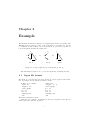
We will mine the TS shown in Fig. 2.1, by splitting the TS into two smaller TSs.
dbminer needs at least two TSs to work (otherwise we recommend to use the
tool rbminer [Sol10, SC10b]), but more partitions are perfectly acceptable, as
long as all partitions share the initial state.
a
s1
s0
a
c
b
s2
=
d
a
s3
s0
s0
∪
s1
b
s2
c
s2
TS A1
TS A
d
a
s3
TS A2
Figure 2.1: A TS A, split into two subsystems A1 and A2 .
The first thing we must do is to create the input files describing the TSs.
2.1
Input file format
The input is a text file that describes the TS as a state graph in SIS format.
For our example the file has the following content:
# This is a comment
.model ts1
.outputs a b
.state graph
s0 a s1
s1 b s2
.marking {s0}
.end
.model ts2
.outputs a c d
.state graph
s0 c s2
s2 a s3
s3 d s0
.marking {s0}
.end
We briefly explain the left file.
First line is a comment. Comments are allowed everywhere in the file but
must begin a line with the # symbol.
5
Next line is optional and declares the name of the model. After that the
set of events is defined. Since the format was originally intended to be used to
describe circuits, events can be declared either as .inputs, .outputs or .dummy.
All of them are considered to be the same by dbminer.
Third line contains the header that marks the beginning of the transitions.
All the transitions are of the form s<int> <event> s<int>, and each line must
contain only a single transition. Finally the initial state is designed to be s0 in
line .marking s0. The file must end with the .end keyword.
Once the TS files (assume their names are ts1.sg and ts2.sg) are available,
we must create the configuration file for dbminer.
In this case, this configuration file looks like this:
0:ts1.sg
1:ts2.sg
shared states
{ 0:s2 1:s2 }
The first two lines indicate the TS files in which the complete TS is partitioned.
The format is always <number>:<filename>, where the number always begins
by zero and is sequentially incremented. These numbers allow to express the
shared states between TSs in a more easy way. Once all TSs have been listed,
they key words shared states indicate the beginning of the shared states section. If no shared state exists (other than the initial state), this part can be
safely skip. Each equivalency group is enclosed between braces and is a list with
the format <number>:s<int>, where the number is the TS number and s<int>
is the state name in that TS. In this example we are saying that state s2 in the
first TS is the same as state s2 in the second state. dbminer does not assume
that states with the same name in different TSs actually refer to the same state,
and must be explicitly stated.
2.2
Using dbminer
Once the configuration file is available, we can call the tool. Since the example
is tiny, we can simply use
dbminer ts.dbm
For bigger examples, usually a bound on the exploration of regions is given. A
typical call would be
dbminer --agg 4 --k 3 big ts.dbm
Indicating that no more that for different basis in the region should be combined
to produce a new region, and that we want a 3-bounded PN.
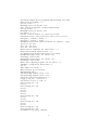
The resulting PN is printed to the standard output, together with lots of
comments informing of the tool progress:
# Reading file: test.dbm
# Parsing succeeded
# Reading file: ts1.sg
#.model|#.outputs|#.state graph|#.end|# Parsing succeeded
# Reading file: ts2.sg
6
#.model|#.outputs|#.state graph|#.end|# Parsing succeeded
#Time used in reading: 0 s.
# Total states: 3
#Finding basis for system ’ts1’
# No conflicts detected, using standard basis
# Total states: 3
#Finding basis for system ’ts2’
# Conflict: 1 1 1
# Final conflict matrix: [1,3]((1/1,1/1,1/1))
# Gradient basis: [2,3]((-1/1,1/1,0/1),(-1/1,0/1,1/1))
# Region 0. Tokens: 0 Power: 1
# Region 1. Tokens: 1 Power: 1
#Compatibility matrix (before reduced row transf.): [3,4]
((1/1,0/1,1/1,1/1),
(1/1,1/1,-1/1,0/1),
(1/1,1/1,-1/1,0/1))
#Time used in computing the final basis: 0 s.
#Time used reading region states: 0 s.
# Computing region basis multisets for each TS
#Computing region basis for system ’ts2’
# Writing ’ts2.bas.bin’
#Computing region basis for system ’ts1’
# Writing ’ts1.bas.bin’
#Time used computing regions for all bases: 0 s.
# Number of regions in union basis: 2
# k = 1
#max number of states: 3
#Basis memory space reserved
#Normalizing bases
# Normalizing regions in TS 0 ts1
# Normalizing regions in TS 1 ts2
# Region r0 has been shifted by 1
# agg: 4 min_val: -1 max_val: 1
# Solution vectors to scan: 8
# Processing TS 0 (1)
# +10%
# Processing TS 1 (4)
# +10%
# +10%
# +10%
# +10%
# Processing TS 0 (4)
# +10%
# +10%
# Processing TS 1 (2)
# +10%
# +10%
# Processing TS 0 (0)
# Processing TS 1 (0)
# Candidate list has 6 elements
7
#Time used computing candidate list: 0 s.(0 s. using timer_t)
# Initial predecessor combination sets created
# Processing TS1
# Removing combinations with predecessor combinations
# 6 Surviving combinations
#Time used to find minimal regions: 0 s.(0 s. using timer_t)
# Started simplification of 0 positive regions
#Total non-redundant positive regions: 0
# Started simplification of 6 nonpositive regions
# Created LP problem with 5 rows and 6 columns
#Total non-redundant regions (after 1st pass): 6
#Total non-redundant regions (after 2nd pass): 4
#Total non-redundant regions (after 3rd pass): 4
.model unionSystem
.outputs a b c d
.graph
a p0
p0 b
p0 d
p1 a
b p1
d p1
p2 b
p2 c
d p2
b p3
c p3
p3 d
.marking {p1 p2}
.end
#Time used computing PN: 0 s.
#Elapsed time: 0 s. (0 s. using timer_t)
The first lines inform of the reading process of the input file. Then, all TS
files appearing in the configuration file are read. Each time the parser finds a
keyword e.g. .state graph prints it so that the user might have some hint of
where problems appear in case of parse failure. After that, the tool computes
the basis of regions of each system and, incrementally, the basis for the whole
system. This basis is distributed among the subsystems and is written down into
files with the .bas.bin extension. Then, the relevant parameters are printed
out before starting the exploration of the region space.
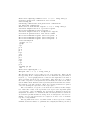
The exact number of regions to scan is shown beforehand, in this example
is 8. Each time a 10% of the regions has been explored, the algorithm prints
a progress line. Since in dbminer the exploration is distributed among the
subsystems, the number of combinations that each subsystem has to start from,
are written in parenthesis when we change from one subsystem to the next one.
Finally, once the exploration has been completed, we have a set of candidate
regions to being minimal.
The algorithm then tries to determine which of these regions are actually
minimal, and then a number of optimizations to simplify the PN are performed,
8
finally printing the resulting PN. The last two lines inform of the time to complete the process. Two ways of computing the time are provided. The first is
more precise (resolution up to 0.01 seconds), but can have overflow problems
when the algorithm is run for a very long period of time. Thus another time
reference is used which is less precise but has no overflow problems.
2.3
Output file format
The output describes a PN in SIS format. In our example this is:
.model unionSystem
.outputs a b c d
.graph
a p0
p0 b
p0 d
p1 a
b p1
d p1
p2 b
p2 c
d p2
b p3
c p3
p3 d
.marking {p1 p2}
.end
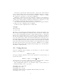
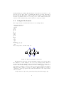
that corresponds to the PN of Fig. 2.2.
a
b
d
c
Figure 2.2: Discovered PN from A1 and A2 .
The first line in the file is optional, indicating a name for the model. Then
the definition of events, similar to the one for the TS input format. The arcs
are declared after the .graph keyword, places must start with p followed by a
number. The initial marking is described in line .marking {p0}. Places not
appearing are assumed to have 0 tokens. If they appear without any further
indication, they contain one token. To assign a different number of tokens a
construction of the type p1=3 is used. More information on the output format
can be found in:
http://www.lsi.upc.edu/~jordicf/petrify/distrib/astg.ps.gz
9
Chapter 3
Utilities
Although dbminer is actually distributed alone, many of the helper tools that
come with its sister tool rbminer [Sol10, SC10b] could be of interest. The most
important among them is the log2ts tool, that converts a log into a TS.
3.1
log2ts
Usage: log2ts [options] log file
The input format of the log is very simple. Each line contains a case, with
events separated with one or more spaces. There is a script, xmltotrace that
converts ProM MXML files to this plain format.
The main options of the tool are:
Option
Semantics
--multiset Makes a multiset conversion, merging states with the
same Parikh vector. By default the conversion produced
is sequential, that is, there is only a single shared state
(the initial one) between all traces.
--cfm
Activates the Common Final Marking reduction [SC10a].
This feature is independent of the
type of analysis.
Since the most optimal conversion is the combination of the multiset and
bisimilar options, the tipical call to this tool is:
log2ts --multiset --cfm log.tr > log.sg
The output is printed to the standard output so it can be redirected as usual.
3.2
conformancecheck
Checks if the given PN can simulate all the traces in the specified trace file.
If some cannot be simulated, the violating trace is printed, together with an
indication of the place that prevented the PN from generating the trace. This
tool can be used to actually verify that a mining algorithm is producing an
overestimation of the behavior.
10
3.3
create mxml
Converts a plain log file into a MXML file that can be read by ProM.
Usage: create xml plain log mxml log
3.4
pntopnml
Converts a PN in SIS format into a PNML file that can be read by ProM.
Usage: pntopnml pn file > pnml file
The output is printed to the standard output so it can be redirected as usual.
3.5
xmltotrace
This is a script that strips all the XML tags from a MXML ProM log file, and
creates a plain trace file, which can be used with log2ts or conformancecheck.
Usage: xmltotrace mxml file > log file
11
Bibliography
[Arn94]
A. Arnold. Finite Transition Systems. Prentice Hall, 1994.
[CKK+ 97] J. Cortadella, M. Kishinevsky, A. Kondratyev, L. Lavagno, and
A. Yakovlev. Petrify: A tool for manipulating concurrent specifications and synthesis of asynchronous controllers. IEICE Trans. on
Information and Systems, E80-D(3):315–325, March 1997.
[DR96]
Jörg Desel and Wolfgang Reisig. The synthesis problem of Petri
nets. Acta Inf., 33(4):297–315, 1996.
[ER90]
A. Ehrenfeucht and G. Rozenberg. Partial (Set) 2-Structures. Part
I, II. Acta Informatica, 27:315–368, 1990.
[Mur89]
T. Murata. Petri Nets: Properties, analysis and applications. Proceedings of the IEEE, pages 541–580, April 1989.
[SC10a]
Marc Solé and Josep Carmona. Process mining from a basis of state
regions. In Petri Nets, volume 6128 of LNCS, pages 226–245, 2010.
[SC10b]
Marc Solé and Josep Carmona. rbminer:: A tool for discovering
Petri nets from transition systems. In ATVA, pages 396–402, 2010.
[Sol10]
Marc Solé. rbminer. http://personals.ac.upc.edu/msole/
homepage/rbminer.html, 2010.
12