Download Using Graph-Grammar Parsing for Automatic

Using Graph-Grammar Parsing for
Automatic Graph Drawing
C.L. McCreary
Dept. of Computer Science and Engineering
Auburn University
C.L. Combs
Equifax Incorporated
Atlanta, Georgia
D.H. Gill
The MITRE Corporation
McLean, Virginia
1.0 Introduction
Directed graphs, or digraphs, are an excellent means of conveying the structure and operation of many types of systems. They are capable of representing not only the overall structure of
such a system, but also the smallest details in a simple and effective way. However, drawing
digraphs by hand can be tedious and time consuming, especially if the number of vertices and arcs
is large. In addition, much time can be spent just trying to plan how the graph should be organized
on the page. These facts reveal the need for an automated system capable of converting a textual
description of a digraph into a well organized and readable drawing of the digraph.
Many researchers have studied this problem and many graph drawing systems have been
developed [see 3 for complete list]. The aesthetic criteria of the systems vary. The objectives may
include requirements of uniform edge length, minimum number of edge crossings, straight edges,
grid drawings (edges are either horizontal or vertical), minimal bends in the edges, minimum area
covered, and display of symmetries. Some limit the input graphs to a particular class such as
planar graphs, trees, graphs with maximum degree of four, or some application-specific graphs
such as petri nets, network representation, digital system schematic diagrams, PERT diagrams,
flowcharts, etc. CG (Clan-based Graph Drawing Tool) is a tool we use for our work with program
dependency graphs. Like dot [10] and its predecessor DAG [9], CG takes a textual description of
an arbitrary directed graph and produces a visual representation of it. CG uses a unique graph
parsing method to determine intrinsic substructures in the graph and to produce a parse tree. The
tree is given attributes that specify the node layout. One example attribute set is presented in this
paper, but the layout can be tailored to suit different aesthetic criteria. CG then uses tree properties
and adapts the work of Suigyama [12], Warfield[ 13], Eens [7] and Farin [8] in routing the edges.
The objectives of the system are to provide an aesthetically pleasing visual layout for arbitrary
directed graphs. CG incorporates techniques to reduce edge crossings, guarantee few bends in
long arcs, and to shorten long arcs whenever possible.
CG is the first graph drawing tool to use a graph grammar as the fundamental structure that
describes the node layout. Brandenburg [1] defines a layout graph grammar as a graph grammar
together with a layout specification. The layout specification associates a finite set of layout
constraints with each production. Our approach is to classify the productions of the graph parse
and associate layout attributes with each production type in the parse tree of the graph.
2.0 Node Layout
The node layout is determined by the combination of (1) parsing of the graph into logically
cohesive subgraphs and (2) defining layout attributes to apply to the resulting parse tree. The parse
is based on a simple graph grammar, and the attributes that are now programmed into CG produce
a layout whose nodes are balanced both vertically and horizontally.
2.1 Graph Decomposition
Clan-based graph decomposition (CGD) is a parse of a directed acyclic graph (DAG) into
a hierarchy of subgraphs. The subgraphs defined by our graph grammar and parse are called clans.
Let G be a DAG. A subset X ! G is a clan iff for all x, y " X and all z " G - X, (a) z is an ancestor
of x iff z is an ancestor of y, and (b) z is a descendant of x iff z is a descendant of y. An alternate
description of a clan depicts it as a subset of vertices where every element not in the subset is
related in the same way (i.e. ancestor, descendant or neither) to each member in the subset. Trivial
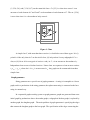
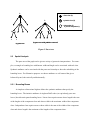
clans include singleton sets and the entire graph. In Figure 1, sets {2,3}, {2,3,4,5,6},
{1,2,3,4,5,6}, and {2,3,4,5,6,7} are the nontrivial clans. C={2,3} is a clan since vertex 1 is an
ancestor of each element of C and 5 and 7 are descendants of each element of C. The set {2,3,4}
is not a clan since 6 is a descendant of only vertex 4.
2
5
3
7
1
4
6
Figure 1. Clans
A simple clan C, with more than three vertices, is classified as one of three types. It is (i)
primitive if the only clans in C are the trivial clans; (ii) independent if every subgraph of C is a
clan; or (iii) linear if for every pair of vertices x and y in C, x is an ancestor or descendant of y.
Independent clans are sets of isolated vertices. Linear clans are sequences of one or more vertices
vi,vi+1,...,vj-1,vj where for i < k, vi is an ancestor of vk. Any graph can be constructed from these
simple clans.
Graph-grammars
String grammars are a special case of graph-grammars. A string is isomorphic to a linear
graph, and in a production of the string grammar, the replacement string is connected to the host
string in a natural way.
In a sequential graph rewriting system or graph-grammar, graphs are generated from some
initial graph by productions where the mother graph, a subgraph of the host graph, is replaced by
another graph, the daughter graph. The main problem of graph-grammars is specifying the edges
that connect the daughter graph to the host graph. The specification of the edges connecting the
daughter graph to the host graph is called the embedding rule. More formally, a graph-grammar
is a system GG = (N, T, z, P, H) where N and T are the nonterminal and terminal vertex labels,
resp., z is a vertex called the axiom or start graph, P is a set of productions and H is an embedding
rule. The particular graph-grammar of the work in this paper is called the clan generation system,
CGS. All host and daughter graphs in CGS are Hasse graphs, i.e. directed graphs with no
transitive edges. The axiom is a single vertex. P is a set of pairs (v,D) where v is any graph vertex
and D is a primitive, independent or linear clan.
For CGS, the reconnection rule or embedding rule is heredity. All host and daughter
graphs in CGS are Hasse graphs, i.e. directed graphs with no transitive edges. An embedding is
called hereditary when in-edges to the mother graph, a single vertex, are replaced with in-edges to
the sources of the daughter graph and out-edges from the mother node are replaced with out-edges
from the sinks of the daughter graph. More formally, let the mother graph be vertex u. For each
vertex v in the set of source vertices in the daughter graph, (w,v) is an edge in the resultant graph
whenever (w,u) is an edge in the host graph. For sink vertices, t, of the daughter graph,(t,w) is an
edge in the resultant graph whenever (u,w) is an edge in the host graph.
6
3
1
6
1
7
5
5
7
2
2
4
4
D
G
G’
m=3
(a)
1
3
4
5
7
1
6
8
2
5
7
4
2
8
6
G
D
m=3
(b)
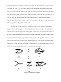
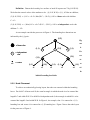
Figure 2. Production examples
G’
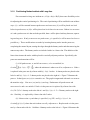
Let us call a production of this system a CGS-production. In applications of
CGS-productions, the daughter graph becomes a clan in the resultant graph. Figure 2 shows
example productions with the mother vertex identified as vertex 3.
Quotient graph
The concept of a quotient graph is important because it permits the classification of
complex clans into the categories of linear, primitive or independent. Let C be a clan and with
{C1,,...Ck} a partition of C where each Ci is a maximal proper subclan of C. The quotient graph
of C denoted C/C1...Ck, is the graph with vertices C1,...,Ck. Pair(Ci,Cj) is an edge of C/C1..Ck iff x
" Ci, y " Cj, and (x,y) is an edge of C. In Figure 1, the clans that partition the entire graph are:
C1 = {1}, C2 = {2,3,4,5,6}, C3 = {7}, and the quotient graph is linear. The clans that partition C2
are {2,3}, {4}, {5}, and {6} and the quotient graph is primitive. Every clan can be identified as
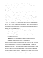
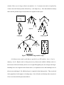
linear, primitive or independent according to the classification of its quotient graph. Figure 3(a)
shows the parse tree of the graph of Figure 1.
Theorem 1: When the original graph is a Hasse graph, the graph generated by
CGS is also a Hasse graph [11].
Theorem 2: Any Hasse graph can be generated by a unique canonical sequence
of productions from CGS [6].
Theorem 3: For every Hasse graph there is a unique decomposition into quotient
graphs that are identified as linear, primitive or independent [5,6].
Theorem 3 guarantees the existence of a unique parse tree from the clans of a graph. In the graph
layout algorithm, the parse tree is used to specify the graph node locations. A bounding box
attribute for each tree vertex, x, specifies the length and width of a rectangle containing the graph
nodes in x’s subtree. The length and width are computed for each linear and each independent
clan from the attributes of the clan’s children. The children of a linear clan are displayed vertically
and the children of a horizontal clan are displayed horizontally in our example layout.
Decomposing Primitives
Primitive clans represent a special challenge. They do not fall into the clear-cut categories
of vertices that should be laid out horizontally or laid out vertically. In addition, primitive clans
can be arbitrarily large, and there can be indefinitely many of them. While this poses no special
challenge to parsing, and every directed graph can be parsed into clans from the three clan types,
arbitrary graph generation is a problem since a list of all primitive graphs must be included in the
production possibilities to create any specific graph. Our approach is to eliminate primitive clans
by decomposing them further into a hierarchy of pseudo-independent and linear clans. By adding
edges from all the source nodes of a primitive to the union of the children of the sources, linear
clan L is formed. L is composed of a clan of the source nodes (which is identified as
pseudo-independent) and the remainder of the primitive clan. The procedure then recursively
parses the remainder of the primitive. This method extracts series-parallel constructs from
primitive clans and represents the serial and parallel structures in the parse tree. The
pseudo-independent clans are treated as independent clans for layout purposes since their nodes
are not connected. The parse tree of any completely decomposed graph is a bipartite tree where
the internal vertices are classified as either linear or (pseudo-) independent. For a connected graph,
the root vertex is always linear. In Figure 1, the primitive {2,3,4,5,6} decomposes into a linear
connection between the independent clans {2,3,4} and {5,6}. The fully decomposed parse tree is
shown in Figure 3(b). The bipartite parse tree can be decorated with layout attributes that can be
synthesized to produce an aesthetically pleasing drawing.
2.2 Extension to Cyclic Graphs
A simple transformation is required to apply the graph decomposition method to cyclic
graphs. Cycles can be found in a depth-first graph traversal. To break a cycle, the arc that identifies
the cycle is given the reverse orientation. When the layout is ready, its orientation will be corrected.
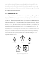
L
= linear clan (L)
!
!
1
2
= independent (I)
or pseudo-independent (i)
7
I
!
= primitive clan (P)
L
P
!
4
!
5
!
6
!
3
(a) parse tree
!
i
1
!
2
!
i
!
!
3
4
!
5
7
!
6
(b) parse tree with primitive removed
Figure 3. Parse trees
2.3
Spatial Analysis
The parse tree of the graph can be given a variety of geometric interpretations. For exam-
ple, a rectangle or bounding box with known width and length can be associated with each clan.
Synthetic attributes can be associated with the parse tree hierarchy to show the embedding of the
bounding boxes. For illustrative purposes we choose attributes we call natural that give a
balanced layout, both vertically and horizontally.
2.3.1 Bounding Boxes
A simple two-dimensional algebra defines the synthetic attributes that specify the
bounding boxes. The intrinsic attributes of singleton DAG nodes (or equivalently parse tree
leaves) describe unit square bounding boxes. Linear clans require an area whose length is the sum
of the lengths of the component clans and whose width is the maximum width of the component
clans. Independent clans require an area whose width is the sum of the widths of the component
clans and whose length is the maximum of the lengths of the component clans.
Definition: Denote the bounding box attribute of node N in parse tree T by (L.N,W.N).
We define the natural values of the attribute to be: (1) (L.N, W.N) = (1,1), if N has no children;
(2) (L.N, W.N) <-- (L.C1+...+L.Ck, Max(W.C1,...,W.Ck)), if N is a linear node with children
C1...Ck;
(3) (L.N, W.N) <--- ( Max(L.C1+...+L.Ck,W.C1,...,W.Ck)), if N is an independent node with
children C1 ...Ck.
As an example consider the parse tree in Figure 4. The bounding box dimensions are
indicated by the (i,j) pairs.
c0
(5,2)
Figure
= linear clan
(1,1)
c1
v0
(3,2)
v6
4.
(1,1)
Pa-
= independent
clan
(3,1)
!
c1
v0
= vertex
(1,1)
!
v1
c2
!
v3
c3
(1,1)
!
(1,1)
v5
(1,1)
!
v2
rse
(2,1)
tr!
(1,1) ee
v4
with
labeled bounding box labels
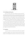
2.3.2 Node Placement
To achieve an aesthetically pleasing layout, the nodes are centered within the bounding
boxes. For child C of linear node N, the actual rectangle in which the node is to be centered has
length L.C and width W.N. For child D of independent node I, the rectangle in which D is to be
centered has length L.I and width W.D. In Figure 4, for example, clan c3 is centered in a (3,1)
bounding box and vertex v0 is centered in a (1,2) bounding box. Figure 5 shows the node layout
for the parse tree of Figure 4.
v0
v1
v2
v3
v4
v5
v6
Figure 5. Bounding boxes
2.3.3 Clan Expansion and Contraction
Since clans are defined as groups of nodes with identical connections to the rest of the
graph, clans can easily be contracted to a single node. Any node not in the clan that was connected
to a clan source or sink will be connected to the contracted node. By allowing segments of the
graph to be contacted, the user can simplify graphs for viewing by contracting those parts which
are not relevant to the investigation. Contracted nodes can be expanded to show the original clan
configuration. Similarly, it is possible to display only the clan, ignoring the rest of the graph.
One of the major differences between the graphs drawn by the naturally attributed CG and
hierarchial systems [12][2] is that the nodes in CG's graphs are spaced in a balanced way both
vertically and horizontally. Hierarchical drawings partition nodes into levels, and all nodes of the
same level are placed on the same horizontal axis. Nodes tend to bunch toward the top of the graph
is these systems. By using our graph decomposition technique, CG is able to determine balanced
vertical spacing as well as balanced horizontal spacing.
3.0 Drawing Arcs
An important consideration that went into the formulation of the arc drawing algorithm
was the question of which pairs of vertices can have arcs between them. The answer lies in the
definition of linear and independent clans. The vertices of a linear clan can have arcs between
them even if the vertices are not consecutive in the clans. Within independent clans no two vertices may be connected by an arc. For these reasons, the algorithm need only consider routing arcs
between vertices within a common linear clan.
There are two major problems to be solved in routing arcs: reducing edge crossings and
“long arc problems”. Producing optimal edge crossings is NP-hard, even for nodes in only two
levels [4]. CG modifies the Barycentric ordering technique of Warfield [13] to be applied to clans,
as well as individual nodes.
The long arc problems include reducing arc lengths whenever possible and the proper
routing of arcs that connect nodes not placed on adjacent levels. To avoid visual conflicts, long
arcs may have to be routed around nodes from intermediate levels. Bends in the arcs are often
necessary for this routing, but may cause visual confusion. Bends should be minimized.
3.1 Routing Long Arcs
Before nodes assume their final position in the layout, their location is determined by considering placement that will shorten long arcs when possible or straighten arcs for those that
cannot be shortened. To describe the method, several definitions are required. The level of node
x, l(x), in DAG G is the length of the longest path from a source to x. The height of node x, h(x),
is the length of the longest path from a sink of the graph to x. The height of DAG G, H(G), is the
maximum of the node heights or, equivalently, the maximum of the node levels. The length of arc
(x,y), L(x,y) = l(y) - l(x). An arc, (x,y),is called long if L(x,y) > 1. Otherwise, it is called short.
Theorem 4: In DAG G, if l(x) + h(x) = H(G), then there exist a path from source
z1 to sink zk, z1,...x=zi,...zk, such that L(zj,zj+1)= 1 for 1 # j < k.
We say a node x is specified if l(x) + h(x) = H(G). The vertical positioning of a specified
node is determined since it is contained in a path whose arcs are all of length 1. Short edges are
routed directly to vertices while long arcs are routed through false vertices embedded in clans
between the two vertices. Since bends are hard to follow and distracting to the eye, our strategy
guarantees that transitive arcs will have at most two bends. Furthermore, no edges will cross long
arcs except possibly at either end of the arc.
3.1.1 Recognizing Long Arcs
A long arc is incident to node x iff there exists node y such that (x,y) "E or (y,x) "E and
$l(y)-l(x)$> 1. If the the long arc, (x,y), is a transitive arc, it is replace by a dummy node z and arcs
(x,z) and (z,y). When the augmented graph is parsed, z is a component in an independent subclan
of the clan containing x and y. The example graph in Figure 6 illustrates this situation. The only
transitive arc is (a,d). Here, node z and arcs (a,z) and (z,d) are added, and arc (a,d) is deleted. The
augmented parse includes new independent clan, {b,c, z} with components {b,c} and {z}. The
augmented parse tree is shown in figure 6d. Since the only role of z is that of place holder for the
dummy node, a reasonable modification of the attribute grammar would be to give the dummy
node a smaller width. The layout in 6(e) illustrates the case where the bounding box of z is
assigned the dimensions (1, 0.5).
a
a
!
!
!
a
d
c
b
b
!
d
b
(a) original graph
d
!
b
c
!
!
!
!
b
!
c
!
z
(d) new parse tree
z
(c) graph with
augmenting
node x
a
d
!
!
!
a
!c
!
c
(b) parse tree
!
!
d
(e) layout
Figure 6. Routing transitive arc
3.1.2
Positioning Nodes Incident with Long Arcs
For non-transitive long arcs incident at x, if l(x) + h(x) < H(G), then some flexibility exists
for adjusting the vertical positioning of x. The vertical positioning will be modified in one of three
ways: (i) x will be centered between predecessor and successor, (ii) x will be placed one level
below its predecessor, or (iii) x will be placed one level above its successor. If there is a successor
of x and a predecessor of x that are both specified, then x will be placed midway between, separating two long arcs. If only a successor or a predecessor, y, is specified, x will be moved as close as
possible to y. These modifications are made by inserting dummy nodes into the parse tree,
completing the normal layout, routing the edges through the dummy nodes and then removing the
unnecessary nodes. The dummy nodes are included with x in a linear clan. The addition of the
linear clans insures the nodes with be placed in vertically adjacent positions. Specifically, the
parse tree transformations will be:
(i) if all predecessors, w, and all successors, z, of x are satisfied, let
d = min
%[l(z) - l(w) - 2] / 2&, where the minimum is taken over all w,z adjacent to x. Node x
is replaced in the parse tree by a linear with l(z) - l(w) -1 nodes: d dummy nodes are placed to the
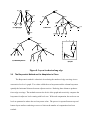
left of x and l(z) - l(w) - d - 2 dummy nodes are placed to the right of x. Figure 7 illustrates the
process. In the figure, arc (a,z) is a transitive arc. The graph is augmented with node x to remove
the transitive edge. Now arcs (x,z) and (e,z) are long. Furthermore all predecessors and
successors of x and e are satisfied. Node x in the parse tree is replaced by a linear clan with
d = (5-0-2)/2 = 1 dummy node to the left of x and l(z) - l(a) - d - 2 = 2 dummy nodes to the right
of x. Similarly, e is replaced by a linear clan with 2 nodes.
(ii) if there exists a y such that y is specified, (x,y) "E, and l(y) - l(x) > 1, let
d = min[l(y)-l(x)-1], where the min is taken over all y adjacent to x. Replace node x in the parse
tree by a linear node with d + 1 children: d dummy nodes to the left of x. Figure 8 illustrates this
solution. Here (a,z) is a long arc that is not transitive. d = 3, and parse tree node a is replaced by
a linear clan with 3 dummy nodes followed by x. (See Figure 8(c)). Note that neither the dummy
nodes nor the potential edges between them are required for the layout.
(5,3) = (length, width)
% = level
!
a
!
1
a
__ = height
!
!
!
b
c
e
0
%
!
2
d
0
!%
z 5
!
5 a
z
!#
x1
c
b
d
!
!
f
g
$
(b) parse tree
f
!
3 d
#
e
!
4 b
#!
4 c
!&
e 1
g
&!
2 f
z
(6,3)
(a) original graph
(c) augmented parse tree
!
(4,3)
!
a
z
!
(4,1)
(4,2)
b
(1,2)
(2,2)
!
d
!
!
b
c
!'
g 1
!
!
!
!
"
x
"
"
!
e
!
!
!
e
(2,1)
a
c
d
"
"
f
!
!
"
"
!g
"
(2,1)
!
"
!
f
!
!
g
(d) augmented parse tree
with dummy linear
z
(e) layout
Figure 7. Layout for long transitive edge
(iii) if there exists a node y such that y is specified, (y,x) "E, and l(x) - l(y) > 1, let d =
min[(l(y)- l(x)-2]. Replace node x in the parse tree by a linear node with d+1 children: node x is
the left-most child and d dummy nodes are to its right. Though the parse tree changes and larger
bounding boxes are assigned to these linear nodes, it is important to leave the bounding boxes of
the ancestors unchanged. No additional space is required for the dummy nodes. They are placed
in the graph only for the purpose of routing edges. Once all nodes and dummy nodes are placed,
all arcs are short and their placement follows.
(0,1)
d (0,4)
a
e
(1,0)
b
g
(1,0) c
(1,3)
z
(1,3)
f
(2,2)
i
(a) original graph
(5,4)
(1,2)
(2,2)
h
0
%
(4,4)
0
%
!
#
!
4 d
1 a
(3,1)
#
3
!
e
(4,2)
!
c
0
(1,2)
(1,2)
(b) Parse Tree
(4,0)
#
!
0 b
#
!
3 f
& !i
1
(1,1)
' !z
0
$!
#!
2 g
2 h
(5,4)
(
(
(
(1,2)
2
!
(
(4,4)
f
!
!
(
e
(4,1)
!
!
(4,2)
!
h!
g!
c
b
(
d
a
!
"
"
"
!
i
a
!
z
!
b
(c) transformed parse tree
!
e
!
f
!
g
i!
(
!
!
!
!
!
h
!
c
!
z
(d) layout
Figure 8. Layout to shorten long edge
3.2
The Barycentric Method and its Adaptation to Clans
The Barycentric method is a heuristic for reducing the number of edge crossings in two
consecutive levels of a graph. Two values called the row barycenter and the column barycenter
quantify the horizontal distance between adjacent vertices. Reducing these distances produces
fewer edge crossings. The method traverses the levels of the graph and recursively computes the
barycenter for adjacent levels starting with level zero. With each computation, the nodes on one
level are permuted to reduce the row barycenter value. The process is repeated between top and
bottom layers until no reordering occurs or a limit on the number of computations has been
reached.
(1,1)
Adapting barycenters to clans involves replacing the adjacent levels of a hierarchy by
adjacent independent clan components of linear clans. The process first inspects the smallest
linear clans in the parse tree (those closest to the leaves). The barycenter method is used on
non-trivial adjacent independent subclans of these linear clans. Once the proper ordering has been
established for the nodes within that linear clan, that ordering remains fixed. The process
continues with the quotient graph where the linear node has been contracted.
Identifying and using only the linear clans results in a significant reduction in the amount
of computation required to perform the barycentric method. In the original barycenter method, the
barycenters are computed on matrices of size ri*ri+1 where ri is the number of vertices in level i
and the computation requires ri*ri+1 multiplications and (ri-1)*ri+1 additions at each level for each
iteration between the top and bottom levels. With the application to the parse tree, after the proper
placement of the independent clans within a linear, there is only one node that represents the entire
structure of the linear clan.
3.3 Smoothing Arcs.
The CG system eliminates sharp corners by using B-splines. When an arc connects an
actual vertex with a dummy vertex, the spline technique described by Enns [7] and Farin [8] is
used. See Figures 9, 10 and 11..
4.0 The Implementation
The CG system has been implemented on a Sun Microsystems SPARCstation running the
SunOS 4.1.2 operating system. It was written in C++ and uses the InterViews toolkit developed
at Stanford University. This toolkit provides an object-oriented interface to the X Window
System. Using this interface, the system generates a drawing of a directed graph from a textual
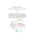
description. The windows in Figures 9, 10, and 11 contain the digraph displays generated by the
CG system. The vertices of the digraph are represented by circles, each of which contains the
number of the vertex. Vertices can be selected by clicking on them with the left mouse button.
This action highlights the vertex by reversing its foreground and background colors. When all the
components of a clan have been selected, the user may then contract the clan. Figure 9 shows a
layout and the results of contracting clans {1, 2} ' {3, 4, 5}, and {6, 7, 8, 9, 10}.
The contracted clans can be selected exactly like the vertices. The expand button can then
be used to expand selected clans to reveal their contents. This expansion and contraction of clans
allows the user to concentrate on specific subgraphs while browsing the digraph.
Figure 9. Graph with 15 nodes and contractions
Figure 10. Random DAG with 33 Nodes
Figure 11. Random DAG with 31 nodes.
References
1. F. J. Brandenburg, "Layout Graph Grammars: the Placement Approach", Lecture Notes in
Computer Science, 532, Graph Grammars and Their Application to Computer Science,
Springer-Verlag, Berlin, 1991..
2. M. J. Carpano, "Automatic Display of Hierarchized Graphs for computer Aided Decision
Analysis", IEEE Trans. on Systems Nab and Cybernetics, vol. SMC-10, no. 11, pp 707-715.
3. G. Di Battista, P. Eades, R. Tamassia, I. Tollis, “Algorithms for Drawing Graphs: an
Annotated Bibliography”, available via ftp from wilma.cs.brown (128.148.33.66) in file
/pub/gdbiblio.tex.Z.
4. P. Eades and N. Wormald, “Edge Crossings in Drawings of Bipartite Graphs”, to appear in
Algorithmica.
5. A. Ehrenfeucht and G. Rozenberg, “Theory of 2-Structures, Part I: Clans, Basic Subclasses, and Morphisms,” Theoretical Computer Science, vol. 70, pp. 277-303, 1990.
6. A. Ehrenfeucht and G. Rozenberg, “Theory of 2-Structures, Part II: Representation
Through Labeled Tree Families,” Theoretical Computer Science, vol. 70, pp. 305-342, 1990.
7. S. Enns, “Free-Form Curves on Your Micro,” BYTE, vol. 11, no. 13, pp. 225-230, Dec.
1986.
8. G. Farin, Curves and Surfaces for Computer Aided Geometric Design. Boston: Academic
Press, 1988.
9. E. R. Gansner, S. C. North, and K. P. Vo, “DAG - A Program that Draws Directed Graphs,”
Software - Practice and Experience, vol 18, no. 11, pp. 1047-1062, Nov. 1988.
10. E. Koutsofios and S. North, "Drawing Graphs with dot", Dot User’s Manual, AT&T Bell
Labs, Murray Hill, N. J.
11. C. L. McCreary, "An algorithm for Parsing a Graph-Grammar, " Ph.D. dissertation, University of Colorado, Boulder, 1987.
12. K. Sugiyama, S. Tagawa, and M. Toda, “Methods for Visual Understanding of Hierarchical System Structures,” IEEE Trans. on Syst., Man, and Cybernetics, vol. 11, no. 2, pp.
109-125, Feb. 1981.
13. J. N. Warfield, “Crossing Theory and Hierarchy Mapping,” IEEE Trans. on Syst., Man,
and Cybernetics, vol. 7, no. 7, pp. 505-523, Jul. 1977.