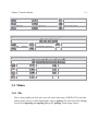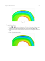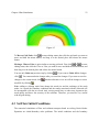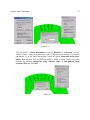
1
NATIONAL CENTER FOR COMPUTATIONAL
HYDROSCIENCE AND ENGINEERING
CCHE2D-GUI – Graphical User Interface for the CCHE2D Model
User’s Manual – Version 2.2
Technical Report No. NCCHE-TR-2005-03
Yaoxin Zhang
School of Engineering
The University of Mississippi
University, MS 38677
May 2005
NATIONAL CENTER FOR COMPUTATIONAL
HYDROSCIENCE AND ENGINEERING
Technical Report No. NCCHE-TR-2005-03
CCHE2D-GUI – Graphical User Interface for the CCHE2D Model
User’s Manual – Version 2.2
Yaoxin Zhang
Post-doctoral Research Associate
The University of Mississippi
May 2005
Table of Contents
1 INTRODUCTION...................................................................................................................... 1
1.1 FAMILY OF CCHE2D MODEL ................................................................................................ 1
1.2 USING THIS MANUAL............................................................................................................. 2
1.3 RELATED DOCUMENTS........................................................................................................... 3
2 CCHE2D MODEL ..................................................................................................................... 4
2.1 NUMERICAL SIMULATION ...................................................................................................... 4
2.1.1 INTRODUCTION ............................................................................................................................ 4
2.1.2 GENERAL PROCEDURE OF USING CCHE2D MODEL ................................................................... 5
2.1.2.1 Mesh Generation.................................................................................................................. 5
2.1.2.2 Boundary Conditions ........................................................................................................... 6
2.1.2.3 Parameter Setting ................................................................................................................. 6
2.1.2.4 Simulation ............................................................................................................................ 6
2.1.2.5 Results Interpretation ........................................................................................................... 6
2.2 CCHE2D MODEL .................................................................................................................. 7
2.2.1 GOVERNING EQUATIONS ............................................................................................................. 7
2.2.2 TURBULENCE CLOSURE ............................................................................................................... 8
2.2.2.1 Eddy Viscosity Model.......................................................................................................... 8
2.2.2.2 Two-dimensional k − ε Model ........................................................................................... 9
2.2.3 SEDIMENT TRANSPORT ................................................................................................................ 9
2.2.3.1 Total Load.......................................................................................................................... 10
2.2.3.2 Non-equilibrium Transport ................................................................................................ 10
2.2.3.3 Bed Material Sorting.......................................................................................................... 10
2.2.3.4 Initial Conditions ............................................................................................................... 11
2.2.3.5 Empirical Formulas............................................................................................................ 11
3 OVERVIEW OF CCHE2D-GUI ............................................................................................ 12
3.1 INTRODUCTION .................................................................................................................... 12
3.2 MAIN WINDOW .................................................................................................................... 12
3.3 TOOLBARS ........................................................................................................................... 13
3.4 MENUS ................................................................................................................................. 14
3.4.1 FILE ............................................................................................................................................ 14
Table of Contents
ii
3.4.2 SIMULATION .............................................................................................................................. 15
3.4.3 VIEW .......................................................................................................................................... 16
3.4.4 SETTINGS ................................................................................................................................... 17
3.4.5 VISUALIZATION ......................................................................................................................... 18
3.4.6 DATA ......................................................................................................................................... 18
3.4.7 HELP .......................................................................................................................................... 18
3.4.8 POPUP MENUS............................................................................................................................ 19
4 RUN SIMULATIONS ............................................................................................................. 20
4.1 INTRODUCTION .................................................................................................................... 20
4.2 EDIT GRID ............................................................................................................................ 21
4.3 SET FLOW INITIAL CONDITIONS ........................................................................................... 23
4.4 SET FLOW PARAMETERS ...................................................................................................... 27
4.5 SET SEDIMENT PARAMETERS ............................................................................................... 32
4.6 SET SEDIMENT BOUNDARY CONDITIONS ............................................................................. 37
4.7 SET INLET/OUTLET BOUNDARY ........................................................................................... 39
4.8 SET BED MATERIAL SAMPLES ............................................................................................. 43
4.9 SET BED MATERIAL PROPERTIES ......................................................................................... 45
4.10 SET MONITOR POINTS ........................................................................................................ 48
4.11 RUN CCHE2D MODEL ...................................................................................................... 49
4.12 USE WIZARD ...................................................................................................................... 52
5 VISUALIZE RESULTS .......................................................................................................... 54
5.1 INTRODUCTION .................................................................................................................... 54
5.2 VISUALIZE FLOW RESULTS .................................................................................................. 54
5.2.1 VISUALIZE INTERMEDIATE AND FINAL RESULTS ...................................................................... 54
5.2.2 VISUALIZE HISTORY FILE .......................................................................................................... 56
5.3 VISUALIZE SEDIMENTS RESULTS ......................................................................................... 58
5.4 PROBE AND EXTRACT DATA ................................................................................................ 60
5.4.1 PROBE DATA .............................................................................................................................. 60
5.4.2 EXTRACT DATA ......................................................................................................................... 64
5.5 SETTINGS ............................................................................................................................. 66
5.5.1 FLOOD PROPERTIES ................................................................................................................... 67
5.5.2 CONTOUR PROPERTIES .............................................................................................................. 68
5.5.3 VECTOR PROPERTIES ................................................................................................................. 71
5.5.4 TEXT .......................................................................................................................................... 72
5.5.5 LEGEND ..................................................................................................................................... 74
5.5.6 BACKGROUND ........................................................................................................................... 75
5.5.7 LAYOUT ..................................................................................................................................... 77
6 APPENDIX: FILE FORMAT ................................................................................................ 78
1 Introduction
1.1 Family of CCHE2D Model
Welcome to the family of CCHE2D model, an integrated package for simulation and
analysis of free surface flows, sediment transport and morphological processes. In addition to
the numerical model itself, this family includes two more members: a mesh generator
(CCHE2D Mesh Generator) and a Graphical Users Interface (CCHE2D-GUI), which will
help you use CCHE2D model more easily and efficiently. The former, the CCHE2D mesh
generator, allows the rapid creation of complex structured mesh systems for CCHE2D model
with several integrated useful techniques and methods, while the latter, the CCHE2D-GUI, is
a graphical users environment for the CCHE2D model with four main functions: preparation
of initial conditions and boundary conditions, preparation of model parameters, run
numerical simulations, and visualization of modeling results.
As illustrated in Fig. 1.1, the CCHE2D Mesh Generator provides meshes for CCHE2D-GUI
and CCHE2D numerical model, while the CCHE2D-GUI provides a graphical interface to
handle the data input and visualization for CCHE2D numerical model.
Chapter 1 Introduction
2
CCHE2D Mesh Generator
Mesh
CCHE2D-GUI
Graphical Users Interface
Input
Output
CCHE2D Numerical Model
Figure 1
1.2 Using This Manual
This manual provides necessary information for using the CCHE2D-GUI, an intergrated 2D
numerical modeling system. It explains in detail how to prepare and edit the initial conditions
and the boundary conditions, how to set the model parameters, how to run CCHE2D model
and how to visualize the modeling results.
This manual is organized as follows:
•
Chapter 2 introduces the CCHE2D numerical model and the fundamentals on
numerical simulation. Users new to numerical modeling are recommended to read
this chapter carefully.
•
Chapter 3 gives an overview of CCHE2D-GUI to make you familiar with the
interactive graphical environment.
Chapter 1 Introduction
3
•
Chapter 4 describes in detail the procedures to run the CCHE2D model through the
GUI. You will learn how to edit grid, set initial conditions for flow, set model
parameters, set the initial bed composition file and sediment boundary conditions
files, set the initial bed material properties, set the monitor points, run simulations.
•
Chapter 5 shows you how to visualize simulation results for flow and sediment
transport, probe and extract data, set the flood properties and contour properties, edit
the texts, set legend properties, and set the background color and background image.
•
The appendix gives you a quick reference to the formats of files the users must
provide for the CCHE2D-GUI.
Readers of this manual may also need to read the manual of CCHE2D Mesh Generator, a
separate program that generates the numerical meshes required to start using the CCHE2DGUI.
1.3 Related Documents
The documentation of CCHE2D is separate into several publications designed to fulfill the
needs of different audiences. They are simply listed as follows:
•
“CCHE2D-GUI Quick Start Guide” is intended for the first-time users.
•
“CCHE2D-GUI – Graphical Users Interface for CCHE2D Model - User’s Manual”
describes in detail the capabilities and How-Tos of CCHE2D-GUI.
•
“CCHE2D: Two-dimensional Hydrodynamic and Sediment Transport Model for
Unsteady Open Channel Flows Over Loose Bed” describes in detail the basic
mathematics, numeric, hydraulics and sediment transport approaches.
•
“CCHE2D Sediment Transport Model” describes in detail the governing equations,
boundary conditions, numerical methods and empirical formulas of the CCHE2D
non-equilibrium transport model of non-uniform sediment.
•
“CCHE2D Mesh Generator Users’ Manual” is aimed at how to generate
computational meshes for the CCHE2D model. It is associated with a separate
software: CCHE2D Mesh Generator.
2 CCHE2D Model
2.1 Numerical Simulation
2.1.1 Introduction
Modeling Free Surface Flows and Sediment Transport with numerical models are much
easier and more efficient than conducting field study in natural waters. One needs only a
computer, a numerical model and the data. However, you may soon find out it takes more
than these to have realistic and meaningful numerical solutions.
Numerical models are established based on the conservation laws and mathematics, it has to
deal with many true physical and mathematical parameters. One has to understand all these
parameters and make sure all the parameters prepared for the simulations are in correct
range.
A numerical model is an approximation of the real world physical processes, even for very
simple physical problems, the accuracy for the simulated quantities such as flow velocities
and water surface elevation is limited. One should understand and expect errors due to
mathematical approximation (Reynolds average, depth-average, and truncation errors, etc)
and physical approximations (vertical flow acceleration is negligible, turbulent closure
schemes, etc) involving in formulating a numerical model. Although numerical model
verification and validation procedures could eliminate possible errors in the computation
code due to mistakes, the errors due to approximations are inevitable.
When a model is applied to field study, one has to calibrate the model with field data.
Because the resistance to the flow is represented by a roughness coefficient which varies with
properties of sediment, bed form, channel geometry, and vegetation, etc., this information has
to be characterized and fit to the model. Calibrating the model and identifying the mean or
distribution of resistance to the flow is always necessary. Since the real world is very
complicated, one normally would not have complete channel roughness information.
Chapter 2 CCHE2D Model
5
Numerical models approximate physical problems, it has however all the components to
represent the physics to be simulated. Mesh or grid is used to represent channels and
bathymetry; inflow and outflow are defined at inlet and outlet sections as boundary
conditions. All the above and model parameters have to be defined before a simulation can
start. To make setting up a simulation case efficiently, a mesh generator and a User Graphic
Interface have been developed.
2.1.2 General Procedure of Using CCHE2D Model
The numerical modeling based on solving the Navier-Stokes equations is an initial-boundary
value problem. Users must provide initial conditions and the boundary conditions. The
general procedure of a numerical simulation can be simply listed as follows:
•
Mesh generation
•
Specification of boundary condition
•
Parameters setting
•
Simulation
•
Results visualization and interpretation.
2.1.2.1 Mesh Generation
A mesh represents a computational domain and the way the governing equations are
discretized. To have a successful simulation, one has to prepare the mesh carefully, so that
the following concerns are taken into consideration:
•
The interested zones has sufficient resolution;
•
Transition between areas of different densities is smooth;
•
Inlet(s) and outlet(s) should be sufficiently far away from the zones of interest;
•
The mesh should be smooth and orthogonal as much as it allows.
Mesh generation particularly for practical problems takes a lot of time, however, the time
shall be paid off if good quality is achieved. In many cases, the simulation code will run with
a low quality mesh but the results maybe less reliable.
Chapter 2 CCHE2D Model
6
2.1.2.2 Boundary Conditions
Computations are conducted in a limited portion of free surface flows, boundary conditions
are the driving mechanisms with which the flow in the simulated area behave. Therefore, one
should set boundary conditions as close to true physics as possible. It is often the
distributions of boundary conditions are unknown (distribution of velocity of discharge in a
cross-section), in these cases, mean flow properties are specified and the inlet and outlet
sections should be set distant from the interested zone.
2.1.2.3 Parameter Setting
Numerical simulation is to reproduce true physics by solving mathematic equations,
therefore, many physical parameters and numerical parameters are needed. Some physical
parameters have been provided in the Graphic User Interface as default which should be
treated as guidance only. Many have to be provided by users for their particular applications.
Users must also provide the parameters that control the simulation processes. The sediment
transport parameters (size distribution of bed materials and loads) often have higher level of
uncertainty then those for the flow; bed roughness parameters are often identified through
calibration which will match the energy slope of the numerical model to the studied physical
subject.
2.1.2.4 Simulation
When the mesh is ready, boundary conditions have specified, one is ready to start a round of
simulation. Since the CCHE2D is a model using a time marching scheme, one should also reexam the initial condition. Because the initial condition for a water flow in natural condition
is unknown, cares have to be taken to make sure the guessed initial condition is reasonable,
particularly for unsteady problems.
Stability is a problem the modeler must aware. When the time step is too large for a
particular problem, the simulation will not continue or it may produce totally unreasonable
results. In these situations, one should reduce the time step used and retry, until the solutions
becomes stable. Although an implicit scheme is used in the CCHE2D model, time step can
not be set arbitrarily.
2.1.2.5 Results Interpretation
It is debatable how much one can trust the obtained numerical simulation results: “Is it
reasonable?” The answer to this is yes and no.
Chapter 2 CCHE2D Model
7
Numerical model is developed under certain assumptions, the results should be reliable if the
simulated flow satisfies these assumptions. However, the natural is always complicated, these
assumptions could never be satisfied one hundred percent. If the results are questioned, we
recommend validating them by comparing with physical model measurements or field data.
Once the model is validated with site specific data, it could be used to study the trend of the
flow or sediment transport processes by varying concerned parameters
2.2 CCHE2D Model
CCHE2D model is a two-dimensional hydrodynamic and sediment transport model for
unsteady open channel flows over loose bed. Here a brief introduction of the CCHE2D
model is presented, its details can be found in Jia and Wang (1999 and 2001).
2.2.1 Governing Equations
The depth integrated two-dimensional equations are solved in CCHE2D model.
Continuity Equation:
∂Z ∂ ( hu ) ∂ ( hv )
+
+
=0
∂t
∂x
∂y
(2.1)
Momentum Equations:
∂u
∂u
∂u
∂Z 1 ∂ ( hτ xx ) ∂ ( hτ xy ) τ bx
+u
+v
= −g
+ [
+
]−
+ f Cor v
∂t
∂x
∂y
∂x h
∂x
∂y
ρh
(2.2)
∂Z 1 ∂ (hτ yx ) ∂ (hτ yy ) τ by
∂v
∂v
∂v
+ [
+
]−
− f Cor u
= −g
+u +v
ρh
∂y h
∂x
∂y
∂y
∂x
∂t
(2.3)
where u and v are the depth-integrated velocity components in the x and y directions
respectively; g is the gravitational acceleration; Z is the water surface elevation; ρ is water
density; h is the local water depth; fCor is the Coriolis parameter; τ xx , τ xy , τ yx and τ yy are the
depth integrated Reynolds stresses; and τ bx and τ by are shear stresses on the bed surface.
Chapter 2 CCHE2D Model
8
2.2.2 Turbulence Closure
In Equations (2.2) and (2.3), the Reynolds stresses are approximated based on Boussinesq’s
assumption:
τ xx = 2ν t
∂u
∂x
(2.4a)
τ xy = τ yx = ν t (
τ yy = 2ν t
∂u ∂v
+ )
∂y ∂x
∂v
∂y
(2.4b)
(2.4c)
2.2.2.1 Eddy Viscosity Model
There are two zero-equation eddy viscosity models adopted in the CCHE2D model. The first
one is the depth-integrated parabolic model, in which the eddy viscosity ν t is calculated by
the following formula:
νt =
Axy
6
κU * h
(2.5)
where Axy is an adjustable coefficient of eddy viscosity, κ is the von Karman constant, and
U * is the shear velocity.
The second eddy viscosity model is the depth-integrated Mixing Length model. The eddy
viscosity ν t is calculated by the following equation.
ν t = l 2 2(
∂U 2
∂u ∂v
∂v
∂u 2
) + 2( ) 2 + ( + ) 2 + (
)
∂z
∂x ∂x
∂x
∂x
(2.6a)
1
1
z
l = ∫ κz (1 − )dz = κh ∫ λ 1 − λ dλ ≈ 0.267κh
h
h
0
(2.6b)
∂U
U*
= Cm
∂z
κh
(2.6c)
where C m is a coefficient with a value of 2.34375 so that Equation (2.6) will cover Equation
(2.5) in the case of a uniform flow in which all the horizontal velocity gradients vanish.
Chapter 2 CCHE2D Model
9
2.2.2.2 Two-dimensional k − ε Model
In this model, differential equations are introduced for the turbulent kinetic energy k and the
∂u ' ∂u i '
1
.
rate of dissipation of turbulent energy ε , where k = ui ' ui ' and ε = µ t i
2
∂x j ∂x j
The depth-integrated governing equations for k and ε are:
∂k
∂k
∂k ∂ ν ∂k
∂ ν ∂k
+u
+v − [ t
]− [ t
] = P − ε + PkV
∂t
∂x
∂y ∂x σ k ∂x ∂y σ k ∂y
(2.7)
∂ε
∂ε
∂ε ∂ ν t ∂ε
∂ ν ∂ε
ε
ε2
+u
+v
− [
]− [ t
] = c1ε P − c 2ε
+ PεV
∂t
∂x
∂y ∂x σ ε ∂x ∂y σ ε ∂y
k
k
(2.8)
where
P = −u ''i u 'j u i , j = ν t [2(
PkV = C k
U *3
h
∂u 2
∂v
∂u ∂v
) + 2( ) 2 + ( + ) 2 ]
∂x
∂y
∂x ∂y
PεV = Cε
U *4
h2
(2.10)
U * = c f (u 2 + v 2 )
Ck =
1
(2.11)
C ε = 3 .6
cf
(2.9)
c 2ε
c 3f / 4
cµ
(2.12)
and c f is the friction coefficient.
From the local values of k and ε , a local eddy viscosity can be evaluated as
νt =
cµ k 2
ε
(2.13)
In the above equations, the following values are used for the empirical constants:
c µ = 0.09, c1ε = 1.45, C 2ε = 1.90, σ k = 1.0, σ ε = 1.3 .
2.2.3 Sediment Transport
A brief introduction of CCHE2D sediment transport is presented here. For details, please
refer to the technical report by Wu (2001).
Chapter 2 CCHE2D Model
10
2.2.3.1 Total Load
According to the conventional classification, moving sediment is divided into suspended load
and bed load along the vertical direction. The bed load is the part of the sediment moving on
or near the bed by rolling, saltating or sliding, while the suspended load moves in
suspensions, which physically occupies the water column along the flow depth above the bed
load layer. For a more general application, the total load sediment transport is simulated in
CCHE2D model.
2.2.3.2 Non-equilibrium Transport
Since the suspended load transport occurs mostly at a non-equilibrium state, it is usually
simulated by non-equilibrium transport models. Different from most existing sediment
transport models that assume a local equilibrium of the bed load transport, the CCHE2D
model implements a full non-equilibrium transport model for both bed load and suspended
load. The depth-integrated convection-diffusion equation of the suspended load transport and
the continuity equation of bed load are solved in CCHE2D model.
2.2.3.3 Bed Material Sorting
The bed material gradation usually varies along the vertical, so the bed material above the
non-erodable layer is divided into several layers, as shown in Figure 2-1. The top layer is the
mixing layer, and the second is the subsurface layer. The variation of bed material gradation
in the mixing layer can be described by a partial differential equation, while in other layers
under the mixing layer the bed material gradation can be determined by using the mass
conservation law.
Figure 2-1
Chapter 2 CCHE2D Model
11
2.2.3.4 Initial Conditions
For a complete simulation of sediment transport, information on sediment properties,
sediment transport capacity, non-equilibrium adaptation length and movable bed roughness
should be given. The sediment properties include the sediment grain size, specific gravity
(default value: 2.65), grain shape factor (default value: 0.7) and bed material porosity. The
sediment transport capacity, non-equilibrium adaptation length and the movable roughness
are determined by empirical formulas.
2.2.3.5 Empirical Formulas
Dozens of formulas for the fractional non-cohesive sediment transport are available.
CCHE2D model selects four formulas or module capable of accounting for the hiding and
exposure effect. The sediment transport capacity is determined by van Rijn’s (1984) formula,
Wu et al’s (2000) formula, SEDTRA module (Garbrecht et al., 1995), the modified Ackers
and White’s formula (Proffit and Sutherland, 1983), or the modified Engelund and Hansen’s
formula (Wu and Vieira, 2000). The effect of secondary flow on the main flow and sediment
transport in curved channels has also been considered in current version of CCHE2D model.
3 Overview of CCHE2D-GUI
3.1 Introduction
This chapter explores the interface of the CCHE2D-GUI. The functions of the main window,
the toolbars, and the menus will be explained in details to help you get familiar with this
interactive graphical environment.
3.2 Main Window
Figure 3-1
Chapter 5 Visualize Results
13
The main window provides an interactive platform for the users. As shown in Fig. 3-1, it
contains all the functional components or the accesses to these components. It is composed of
the title bar (displays the file path to the data set), the menu bar, the toolbars (main toolbar
and editing toolbars), the status bar, and the plot area.
3.3 Toolbars
Main Toolbar
Incremental Zoom Out
Plot Flood and Lines
Open a Geo File
Add/Remove XY Axis
Plot Points
Save as a Layout File
Add/Remove Legend
About
Print Current Image
Add/Remove Title
Simulation Wizards
Show/Hide
Run simulations
Add Texts
Select Pointer
Data Probe
Zoom In
Grid On/Off
Pan
Vector On/Off
Zoom To Full Size
Plot Flood Contour
Incremental Zoom In
Plot Contour Line
Display variable
Background
Show/Hide Simulation Time
Show/Hide Dry Area
Toolbar for Grid Editing
Start/Stop Grid Editing
Delete I Line
Undo Previous Change
Chapter 5 Visualize Results
14
Add J Line
Move Grid Node
Undo All Changes
Delete J Line
Move J Line
Save All Changes
Add I Line
Move I Line
Save as a New Geo File
Toolbar for Boundary Editing
Start/Stop
Add
Delete Boundary Node String
Boundary
Modify Boundary Node String
Select Boundary Node String
Toolbar for Background Image Editing
Start/Stop Editing
Rotate Right
Downward Translation
Zoom In Image
Left Translation
Translation
Zoom Out Image
Right Translation
Set Transformation Parameters
Rotate Left
Upward Translation
3.4 Menus
3.4.1 File
This is most probably the first menu you will touch when using CCHE2D-GUI. It provides
almost all the accesses to files Input/Output, such as opening Geo and Layout files, saving
Layout files, importing and exporting Bitmap file, printing current image, and etc.
Chapter 5 Visualize Results
15
Figure 3-2
3.4.2 Simulation
After loading the Geo mesh file, you need to visit this menu to run simulations. According to
the functions, the menu items are divided into four groups, “wizard” group, “run” group”,
“flow” group and “sediment” group (see Figure 3-3).
In “wizard” group, it provides you a quick guide on how to run simulations.
In “run” group, it provides you access to run simulations, i.e., Run CCHE2D Model….
In “flow” group, it provides you editing tools to prepare the initial conditions, boundary
conditions and the model parameters for flow.
In “sediment” group, it provides you editing tools to prepare the initial conditions, boundary
conditions and the model parameters for sediment.
Chapter 5 Visualize Results
16
Figure 3-3
3.4.3 View
This menu provides you necessary tools to view the current image more clearly and
accurately, such as Select, Zoom, and Pan, etc.
Figure 3-4
Chapter 5 Visualize Results
17
3.4.4 Settings
Visiting this menu, you can set up the visualization styles best fit your needs and personality,
such as plot type, colors, adding text, showing/hiding legend, title, grid, boundary,
simulation time, vectors, and etc. You can also set up all kinds of visualization
parameters/properties, such as properties of legend, title, text, flood, contour, vector,
background image, and etc.
Figure 3-5
Chapter 5 Visualize Results
18
3.4.5 Visualization
Through this menu, you can visualize all kinds of available result files, the intermediate file,
the final results file, and the history file.
Figure 3-6
3.4.6 Data
You can probe and extract data from the image using this menu.
Figure 3-7
3.4.7 Help
Have any difficulties? Found any bugs? Any comments? Contact us! Your suggestions and
critics are very important to us
Chapter 3 Overview of CCHE2D-GUI
3.4.8 Popup Menus
As shown in Figure 3-8, there are two popup menus: “toolbar” menu and “view” menu.
The “toolbar” popup menu is a copy of the submenu “Toolbar” in menu “View”, while the
“View” popup menu is a simplified version of menu “View” for easy access. The former can
be activated by right clicking the toolbar, while the latter will appear by right clicking the
plot area.
Figure 3-8
4 Run Simulations
4.1 Introduction
One main function of the CCHE2D-GUI is to run simulations using CCHE2D numerical
model. Basically, there are five steps to run simulations. The first step in getting a case ready
for simulation is to generate a mesh for the domain of interest. A mesh file, a file with a
“.geo” extension, is required by both the CCHE2D-GUI and the CCHE2D numerical model.
You need the help of the CCHE2D Mesh Generator. The mesh file contains the geometry and
the initial conditions of the grid, such as the (x,y) coordinates, the initial bed elevation, the
initial water surface level, the bed roughness and the nodal type. In this manual, it is
assumed that you already have such a mesh file.
After loading the mesh file, you can set the initial conditions for flow, including editing the
grid (refining, coarsening, and modifying nodal type), setting the initial bed elevation, the
initial water surface level and the initial bed roughness.
After generating and editing the mesh, the next step is to set the model parameters. The
parameters are divided into two groups: flow parameters and sediment parameters. In flow
parameters, you need to set the simulation parameters, the bed roughness and the general
physical properties of water. In the sediment parameters, you need to define the sediment size
classes, set the transport mode, the transport equations or formulas, and the sediment
simulation options and parameters, etc.
Once the mesh generation process is complete and parameters for flow and sediment are set,
you need to specify proper initial and boundary conditions. If sediment transport option is
desired, you must specify initial composition of the bed. You can specify multiple inlet and
outlet sections for the domain, prescribe specific discharge, total discharge, or discharge
hydrograph at the inlet sections. At outlet sections, you can prescribe a constant water surface
level, a open boundary condition, a rating curve, or a stage hydrograph. In addition, you can
prescribe either steady or unsteady sediment boundary condition at the inlets.
After all the above steps are finished, the last step is to run simulation. You can run the
CCHE2D model locally, that is on the same computer you are running the CCHE2D-GUI.
Chapter 4 Run Simulations
21
4.2 Edit Grid
The CCHE2D-GUI provides basic grid editing functionality that can be used for small
modifications of the computational mesh. You should use the CCHE2D Mesh Generator to
create the best possible mesh, and then import it into the CCHE2D-GUI.
After opening a mesh file, you can go to menu Edit and click Start Editing in submenu Edit
Grid or click
to activate the toolbar for grid editing. The detailed explanations on each
button of the toolbar can be found in chapter 3. You can make some fine tuning of the mesh
before running simulations, such as adding or deleting mesh lines in either I or J direction,
moving grid node, and moving I line and J line. If you want to regenerate the mesh, you need
to use the CCHE2D Mesh Generator.
Figure 4-1
To Add or Delete J Line,
•
•
•
Click
or
to enter the editing status. The I lines of the mesh will become gray
while the J lines will become highlighted. The cursor will become
or
.
Click the desired place (actually somewhere in between two existing J lines) to add a
J line.
Click the J line you want to delete.
Chapter 4 Run Simulations
22
Figure 4-2
To Add or Delete I Line,
•
•
•
Click
or
to enter the editing status. The J lines of the mesh will become gray
while the I lines will become highlighted. The cursor will become
or
.
Click the desired place (actually somewhere in between two existing I lines) to add an
I line.
Click a I line you want to delete.
Chapter 4 Run Simulations
23
Figure 4-3
To Move a Grid Node, click
to enter editing status; then click the grid node you want to
move and hold the mouse button; and drag it to the desired place and release the mouse
button.
Moving a J line or I line is quite similar to moving grid node. First click
or
to enter
editing status; then click the J line or I line you want to move and hold the mouse botton; and
then drag it to the desired place and release the mouse button.
You can only Undo one previous step by clicking
click
. If you want to Undo All the changes,
. You cannot undo the changes after you saved the changes. If you want to save the
changes to the current mesh, click
mesh file by clicking
. Another alternative is to save all the changes to a new
.
Note: adding or deleting mesh lines change the mesh size and the orderings of the mesh
nodes. As a result, the boundary conditions and the results associated with the old mesh will
be incompatible with the new mesh. And, moving mesh lines or nodes may degenerate the
mesh quality and hence the accuracy of the solutions. Therefore, you must be very careful
with the grid editing.
4.3 Set Flow Initial Conditions
The numerical simulations of flow and sediment transport based on solving Navier-Stokes
Equations are initial-boundary value problems. The initial conditions and the boundary
Chapter 4 Run Simulations
24
conditions must be specified before running the simulations. The initial conditions are very
important, since inappropriate initial conditions may slow down the convergence process or
even cause the simulation to fail. The initial conditions include the flow initial conditions and
the sediment initial conditions. This section will tell you how to set the flow initial
conditions.
In addition to the geometry information, the mesh file also contains the information of the
initial flow conditions that include the initial water surface level, bed roughness, and initial
bed elevation. To set the initial conditions for flow, you need to visit Set Flow Initial
Conditions…in Simulation menu which activates the Nodal Properties dialog window.
To Specify Initial Water Surface Level, Roughness and Bed Elevation,
•
Select the flow variable you want to specify by checking the radio button in Assign
WSL, Roughness or Bed Elevation.
•
If you click Whole Domain, the selected flow variable will be assigned a constant
value through the domain.
•
You can also give a spatial distribution to the selected flow variable by clicking SubRegion. After clicking this button, the GUI waits for you to define the region by
selecting two points which defines a rectangular area within the mesh.
•
The Assign Value dialog will appear right after clicking Whole Domain or after you
click the second point when defining Sub-Region. Enter the desired value and click
OK.
•
You can repeat the above steps until the initial conditions of all the flow variables are
set.
•
Note: Please make sure the initial water level at the inlets is higher than bed.
•
Tip: If the initial WSL is too low, there will be many dry nodes at the beginning
of the simulation. This may cause the simulation fail. To avoid it, specify the
initial WSL a little higher to reduce the number of dry nodes.
Chapter 4 Run Simulations
25
Figure 4-4
You can specify a linear distribution in either I direction or J direction of water
surface level in a region represented by a pair of diagonal points instead of a constant
distribution. To do the linear interpolation, check the option Interpolate initial water
surface level and then click two different points to define a region. Finally choose the
direction by checking Interpolate along constant I-lines or Interpolation along
constant J-lines and click OK.
Figure 4-5
Chapter 4 Run Simulations
26
Three nodal types, namely, internal nodes, boundary nodes, and external nodes, are
identified in CCHE2D model. You can change the nodal type for a specified region
represented by a pair of diagonal points. For example, if you want to construct an island in
the domain, follow the following steps:
•
Click the radio button Assign new ID to nodes and then select a region by clicking
on two different nodes.
•
Check the option Set as boundary and click OK. The region will be surrounded by
the blue lines.
•
Click two diagonal points to specify the region covering all the other nodes within the
blue lines.
•
Check the option Set as external and click OK.
•
Warning: You must be very careful when changing the nodal type. It may result
in an ill-defined mesh and the model may fail to run. Each time when you want
to construct an island, make sure follow the above correct steps. You should
always use the CCHE2D Mesh Generator to create high quality mesh.
Chapter 4 Run Simulations
27
Figure 4-6
4.4 Set Flow Parameters
The flow parameters consist of Simulation parameters, Bed Roughness parameters and
Advanced parameters. The Set Flow Parameters window can be invoked by clicking Set
Flow Parameters…in menu Simulation.
In page Simulation Parameters, the parameters are divided into five groups. Each parameter
is explained as follows:
•
In group Time Step,
Chapter 4 Run Simulations
28
o Simulation time (s): the total time period in seconds of the simulation. In
case of steady flow, this time should be sufficient so that a steady solution
could be achieved
o Time step (s): the step for time marching of the simulation.
•
In group Time Step for Output, you can set the step intervals to output results into
the Intermediate File, the History File, and for the Monitor Points, and set the step
intervals for screen outputs indicating Convergence process.
•
In group Turbulence, there are three Turbulence Model Options:
o For Parabolic Eddy Viscosity Model and Mixing Length Model, you can
set the Turbulence viscosity coefficient. This coefficient serves as a
multiplier, i.e., a value of 10 means that the turbulent viscosity is 10 times that
computed from the selected turbulence model. Although normally it equals 1,
this coefficient has been tested in a range of [0.1, 1000].
•
In group Unsteady Flow Computation, you can choose to Compute as quasisteady flow instead of the real unsteady flow. If the flow boundary condition at any
of the inlet section is unsteady, i.e., discharge hydrograph is specified, both the
sediment and flow time steps are the same and the flow and sediment transport
simulations are performed for each time step. However, for long-term simulation the
computation time may be quite long. To increase the computation efficiency, the user
has the choice to turn on the option that computes the unsteady flow as quasi-steady
flow. In this case, the discharge hydrograph provided by the user must be a step
function. The discharge during each step is considered as constant and the flow and
sediment simulations are performed as for steady flow. Suppose (Qi, Ti) and (Qi+1,
Ti+1) represents two consecutive hydrograph ordinates then for quasi-steady
computation the discharge Qi is assumed to be valid for the duration between Ti and
Ti+1. In case of unsteady flow computation, the discharge is interpolated for any time
between Ti and Ti+1. You can set the Time steps to reach steady state during each
step. Note that the time series in the hydrograph files of the inlets and outlets
must be the same. The quasi-steady simulation cannot start from rest and must
run from some base result.
•
In group Numerical,
o Wall slipness coefficient: It is used to specify the wall boundary condition at
no-flow boundaries. A value of 0.0 means no slip condition and a value of 1.0
means total slip, i.e., tangential velocity at no flow boundaries is allowed. A
value between 0.0 and 1.0 would mean partial slip. A value greater than 1.0
Chapter 4 Run Simulations
29
signals the application of log-law. The log-law boundary condition allows
partial slip, however, the shear stress is accurately predicted.
o Depth to consider dry (m): It is used to determine the wet and dry nodes.
The minimum water depth above it used to consider a node to be wet, while
the water depth below that value would make a node dry.
o Time Iteration Method: This parameter provides information about the
number of internal interations per time step. The Method 1, Method 2 and
Method 3 mean small, medium, and large number of iterations per time step.
The actual number is set by the computational model. The value should be
based on the time step size, i.e., if the time step size is large the iteration
control flag should be set to a higher value.
Figure 4-7
In page Bed Roughness, the parameters are divided into two groups: For Flow Simulation
Only and For Sediment Transport Simulation.
Chapter 4 Run Simulations
•
30
For flow simulation, you can choose to either Use Values in .geo File or Use Bed
Roughness Formula. The roughness value in Geo file can be either Manning’s n or
Roughness height Ks. You must specify if the roughness values in the .geo file are
Manning’s n or roughness height.
o Two bed roughness formulas are available for calculation: Wu and Wang
(1999); and van Rijn (1986). If you choose roughness formula for flow, the
selected formula will be also used in the bed roughness calculation for
sediment. You also need to specify the formula parameters, such as D16, D50,
D90 and Calibration Factor. The Calibration Factor is within the range of
[0.2, 5.0] and its default value is 1.0
•
For sediment transport simulation, there are five methods to calculate the bed
roughness. You can Use the value in *.geo file, or calculate bed roughness according
to the sediment diameter size of D90 or D50, or use Wu and Wang (1999)’s formula
and van Rijn (1986)’s formula.
•
The options Wu and Wang (1999) and van Rijn (1986) can be set in either group
For Flow Simulation Only or For Sediment Transport Simulation. Setting them
in one group equals to setting them in both groups at the same time.
Chapter 4 Run Simulations
31
Figure 4-8
In page Advanced, there are four parameters, namely, Coriolis force coefficient,
gravitational acceleration, von Karman constant, and kinematic viscosity of fluid, with
default values that suffice for most cases, however, if needed you can change the default
values.
Chapter 4 Run Simulations
32
Figure 4-9
4.5 Set Sediment Parameters
To run sediment transport simulation, you must specify the sediment parameters and the
initial and boundary conditions. The basic procedure of setting sediment information is listed
as follows:
•
Define the number of layers.
•
Define the sediment size classes. All bed material and boundary condition data are
specified according to these classes.
•
Specify the sediment boundary conditions.
•
Define the bed material samples.
•
Set the bed material properties.
Sediment parameters are specified through the Set Sediment Parameters… in the
Simulations page. There are four pages, Sediment Size Classes, Sediment Transport,
Sediment, and Bed Roughness.
In page Sediment Size Classes,
Chapter 4 Run Simulations
33
•
Number of Bed Layers: is used to define the bed configurations in vertical direction.
The default value is 3. The first top layer is the mixing layer where the exchanges
between sediments in water and on bed occur.
•
Minimum Mixing Layer Thickness: is a numerical parameter used to confine the
bed erosion process.
•
In group Define Size Class,
o To add a size class, input the sediment size diameter one at a time and click
Add Size Class.
o To delete a size class, select a sediment size in Mean diameter (m) of each
size class and click Delete Size Class.
o To delete all size classes, click Clear All.
o Notes: The maximum number of sediment size classes is 8. Practically this
number should not be more than 5, otherwise the computational
efficiency will be reduced significantly.
Figure 4-10
In page Sediment Transport, four groups of parameters need to be specified.
Chapter 4 Run Simulations
•
34
In the first group, you can set the Transport Mode and the Transport Capacity
Formula. There are five transport modes and four capacity formulas available.
o Total Load as Bed Load Plus Suspended Load Model is for simulation of
both the bed load and the suspended load (total load).
o Total Load as Bed Load Model is for simulation of both the bed load and the
suspended load but with the bed load dominant.
o Total Load as Suspended Load Model is for simulation of both the bed load
and the suspended load but with the suspended load dominant.
o If you select Total Load as Bed Load Model or Total Load as Suspended
Load Model, you need to choose appropriate sediment transport capacity
formula.
•
In group Sediment Simulation Mode, two simulation modes are available. The first
option Slow Bed Change can be selected only if the flow is steady, while the option
Fast Bed Change is for unsteady flow. Note that if you choose to Compute as
quasi-steady flow in page Simulation Parameters of Set Flow Parameters (please
refer to section 4.4 for details), it implies the simulation mode of Fast Bed Change for
sediment transport and you will not be able to set other simulation mode.
•
In group Adaptation Length for Bedload, you can choose appropriate option to
calculate adaptation length for bed load for non-equilibrium sediment transport.
•
In group Adaptation Length Factor for Suspended Load, similarly, you can choose
appropriate option to calculate the adaptation length factor for suspended.
•
The non-equilibrium adaptation length characterizes the distance for sediment to
adjust from a non-equilibrium state to an equilibrium state. It is a length scale for the
river bed to respond the disturbance of the environment, such as hydraulic structures,
channel geometry changes and incoming sediment variation.
Chapter 4 Run Simulations
35
Figure 4-11
In page Sediment,
•
The Sediment specific gravity has a default value of 2.65 that suffices for most
applications.
•
The Curvature Effects can be included into the sediment transport simulation if the
domain has the curved parts. You need to set the Average channel width
accordingly.
•
In group Steady Flow Computation,
o The Time steps to adjust flow is used to adjust the flow after the bed
changes. The flow will be recalculated for the number of time steps specified
by the user.
o The Erosion/Deposition limit (0.01-0.05 of depth) is used to restrict the
maximum amount of erosion/deposition in the domain within a time step. If
erosion/deposition at any node within a time step exceeds the limit specified
by the user, the time step is reduced and computations are repeated.
o The above parameters are effective only if steady flow boundary conditions
are prescribed at all the inlets.
Chapter 4 Run Simulations
36
Figure 4-12
The page Bed Roughness is the same as the page Bed Roughness in Set Flow Parameters.
Please refer to section 4.4 for details.
Chapter 4 Run Simulations
37
Figure 4-13
4.6 Set Sediment Boundary Conditions
The information of sediment boundary conditions are provided by the suspended sediment
boundary condition file (*.sbc) and the bedload boundary condition file (*.bbc). The
CCHE2D-GUI provides a file editor to help you edit these two files.
•
To edit these two files, select Set Sediment Boundary Conditions…in menu
Simulations. Please make sure you already defined the sediment size class, otherwise
an error message will appear.
•
In the File Editor, you can create (New), Import and Save the sediment boundary
conditions file selected from the File Selector.
Chapter 4 Run Simulations
38
Figure 4-14
•
To import an existing selected file, click Import.
•
To save the changes to a selected file, click Save.
Figure 4-15
•
To create a template for the selected file, click New. The sbc and bbc template is
created based on the Number of Size Classes and Number of Data Points. The
Number of Size Classes is a predefined value and you cannot set it here. The
Number of Data Points defines the number of time series points. The sbc and bbc
Chapter 4 Run Simulations
39
files have the same format. The unit of Sediment Discharge in sbc is kg / m 3 while
in bbc is kg / s .
•
To edit the cell value, click the active cell and then type the desired values. The cells
in gray color are inactive. You can Cut, Copy, Paste and Delete by right clicking the
selected cells to invoke the popup edit menu.
Figure 4-16
•
Note that once the Number of Data Points is set, you cannot add more data points by
directly inputting values into cells. The sum of the factions of the size classes at each
time series should be 1, other wise an error message will appear.
Figure 4-17
4.7 Set Inlet/Outlet Boundary
To set inlet or outlet boundary conditions, there are two steps to follow: editing boundary
node strings and attaching boundary conditions to the node strings. You need help from the
tools of editing boundary conditions which can be activated by clicking Start Editing
Chapter 4 Run Simulations
40
Inlet/Outlet Boundary from menu Simulation or button
toolbar
on the boundary editing
.
There are two kinds of boundary node strings, inlet boundary node string (denoted by an
arrow entering the domain), outlet boundary node string (denoted by an arrow going out of
the domain).
Figure 4-18
•
To add a boundary node string: click
and then click two different points along
a constant I line or J line. Make sure the node string is at least three nodes wide.
•
To delete a boundary node string: click
to delete.
•
To modify a boundary node string: click
and then click a point on the I line or J
line on which the node string is located. The length of the node string will be
changed. You also need to make sure the modified node string is at least three nodes
wide.
•
To select a boundary node string: click
and then click the desired node string. If
it is inlet boundary node string, you need to attach the Inlet Boundary Conditions; if
it is an outlet boundary node string, you need to attach the Outlet Flow Boundary
Conditions; and if it is a newly added node string, you need to determine its
boundary type in Select Inlet/Outlet Boundary.
Figure 4-19
and then click the node string you want
Chapter 4 Run Simulations
41
For Inlet Boundary Conditions, you need to set the flow inlet boundary conditions and the
sediment inlet boundary conditions.
•
In page Flow,
o You can specify either Total discharge or Discharge hydrograph with
Inflow angle (degree) at the inlet. If the Discharge hydrograph is selected,
you need to provide a discharge hydrograph file (*.dhg) whose file format can
be found in Appendix. Note that the hydrograph must start from t = 0.
o A shortcut of Set Flow Parameters…is provided here. For details, please
refer to section 4.4.
o To detach a flow boundary condition, click Delete Flow BC.
Figure 4-20
•
In page Sediment, you need to provide a bed load boundary condition file (*.bbc) or
a suspended load boundary condition file (*.sbc) or both, which depends on the
option you selected in the Transport Mode of page Sediment Transport in Set
Sediment Parameters.
o To attach an existing sediment boundary condition, click Import BC File…
in group BedLoad Sediment or Suspended Sediment. If no existing
sediment boundary condition is available, you can create a new sediment
boundary condition by clicking Create BC File….and the File Editor will
appear. For details on how to edit sediment boundary conditions using File
Editor, please refer to section 4.6.
Chapter 4 Run Simulations
42
Figure 4-21
o To detach a sediment boundary condition, click Delete Sediment BC.
For Outlet Boundary Conditions, four kinds of outlet flow boundary conditions are
available, Open boundary conditions, Water surface level, Rating curve and Stage
Hydrograph.
•
In case of Open Boundary Conditions, the model will estimate the water surface
level at the outlet boundary based on kinematic wave condition. This option is
valuable if you cannot assess the water level at the channel outlet.
•
If you select Rating curve, you need to provide a rating curve file (*.rcv) with stagedischarge relationship. Please see the Appendix for instructions.
•
If you select Stage hydrograph, you need to provide a stage hydrograph file (*.shg)
with time-stage relationship. Note that the stage hydrograph must start from t = 0.
Chapter 4 Run Simulations
43
Figure 4-22
4.8 Set Bed Material Samples
The bed material samples will be used to define the initial bed material compositions in both
horizontal and vertical directions for the entire domain. The information of the bed material
samples are contained in a file with the extension bmt. To set bed material samples, select
Set Bed Material Samples… in menu Simulation. Please make sure you already define the
sediment size classes, otherwise an error message will appear.
In Define Bed Material Samples,
Chapter 4 Run Simulations
44
•
If the bmt file exists, the defined bed samples will be displayed, otherwise a blank
sheet is displayed.
•
You need to set the Porosity and the fractions of each sample. You don’t need to set
the Sample No.
Figure 4-23
•
To create a new sample, click Add Sample. A sample with default porosity and
equal-distributed factions will be added at the end of the records.
•
To edit a sample, click the corresponding cell and type the desired value. Please make
sure the sum of the factions of each sample be 1, otherwise an error message will
appear.
Chapter 4 Run Simulations
•
45
To save the samples, click OK. The defined bed samples will be saved into the bmt
file and a bed file which defines the initial bed material composition for each mesh
node will be created at the same time using the information from the bmt file. If the
bed file is already existing, you need to confirm if it is overwritten or not.
Figure 4-24
•
To delete all samples, click Reset.
4.9 Set Bed Material Properties
After the bed samples are defined, you can set the initial bed material properties contained in
a file with the extension bed. To set the bed material properties, select Set Bed Material
Properties…in menu Simulation. If the information in bmt file and bed file is not
compatible, you can create a new bed file based on the information from bmt file.
Figure 4-25
There are five properties divided into two groups for each mesh node, Layer Thickness, Bed
Sample Number, Erodibility, Maximum Erosion Thickness, and Maximum Deposition
Thickness.
Chapter 4 Run Simulations
46
Figure 4-26
In group Layer properties,
•
You must set the layer thickness and layer sample number for each layer. The Layer
Number is set in page Sediment Size Classes in Set Sediment Parameters (please
refer to section 4.5). The samples are set in Define Bed Material Samples (please
refer to section 4.8).
•
To set the layer thickness or layer sample number, type the desired value or select
desired sample, then click Whole Domain or Define Distribution. If you click
Whole Domain, the selected property will be assigned a constant value for each
node. You can also give a spatial distribution to the selected property by clicking
Define Distribution. After clicking this button, the GUI expects you to define the
region by selecting two points which are the diagonal points of a rectangular area
within the mesh.
Chapter 4 Run Simulations
47
Figure 4-27
Note that you need to specify the layer properties for EACH LAYER.
In group Nodal Erodibility and Thickness,
•
The erodibility helps differentiate the non-erodible and the erodible nodes. For
example, the nodes on the concrete hydraulic structure should be non-erodible.
•
The Maximum Erosion Thickness and Maximum Deposition Thickness are used
to limit the erosion and deposition process, respectively. By default, a uniform value
of 90 meter is used, that is, no limit is enforced.
•
For a selected property, you can set a constant distribution by clicking Whole
Domain. You can define the distribution by clicking Define Distribution. After
clicking this button, the GUI is waiting for you to define the region by selecting two
points which are the diagonal points of a rectangular area from the mesh.
To save your settings, click Save. The changes will be saved into the bed file.
To undo the changes of the previous step, click Undo.
Chapter 4 Run Simulations
48
To undo all the changes, click Undo All.
4.10 Set Monitor Points
Monitor points are used to get history of results at selected nodes. The current version of the
CCHE2D model allows up to five monitor points in the computational domain. As the
CCHE2D model is an unsteady flow model, even the steady state is attained through forward
marching in time. Thus monitor points are valid both for the steady and unsteady flow
simulation. To set the monitor points, select Edit Monitor Points… in menu Simulation.
•
To add monitor points through IJ Indices, input the I index and J index and then
click Add Point in group Monitor Point Indices.
•
To Add monitor points through Coordinates, input x coordinate and y coordinate
and then click Add Point in Monitor Point Coordinate. A grid point closest to this
location (x, y) will be added.
•
You can also click Add Points from Grid and then click a grid point.
•
You can also click Select Monitor Point and then click the desired place on the
mesh. A grid point closest to this point will be added as a monitor point.
•
You can Remove Current Point and Remove All Points
•
To save the monitor points, Click Save.
•
If you set the monitor points, you need to set time step for monitor points output on
page Simulation in Set Flow Parameters.
Chapter 4 Run Simulations
49
Figure 4-28
4.11 Run CCHE2D Model
After all the initial conditions and the boundary conditions are set, the simulation can be
performed. To run CCHE2D model locally, select Run CCHE2D Model… in menu
Simulation or click
in the main toolbar.
In Simulation Options, the current Run Number is displayed at the top of the window. This
Run Number will be used to name the corresponding results file. The flow result file has the
extension “flw”, while the sediment result file has the extension “sdm”. The name of the
result file has the following generic form:
CaseName_Run-Current Run Number (Start Run Number).flw (or sdm)
For example, if the CaseName is “try”, the Current Run Number is 4, and the Start Run
Number is 1, the result file will be: “try_Run-4(1).flw” or “try_Run-4(1).sdm”. The Start Run
Number represents the results from the corresponding run. If it is 0, it means the simulation
will begin from rest.
There are four simulation options.
Chapter 4 Run Simulations
•
50
Start Flow Simulation from Rest: It is also called “cold start” for flow simulation.
The flow simulation will begin with the initial water surface specified as in section
4.3 and the initial velocity field (velocities are set to zero by default)
.
Figure 4-29
•
Continue Flow Simulation from Flow Filed at Time: It is also called “hot start” for
flow simulation. The flow simulation will begin with the computed flow field at a
selected time. You can select the flow field from the corresponding flow filed
selector.
Figure 4-30
Chapter 4 Run Simulations
•
51
Start Sediment Transport using Flow Field at Time: It is also called “cold start”
for sediment transport simulation. The sediment transport will begin with the initial
bed defined in the mesh file (geo) and the computed flow field at a selected time. You
can select the flow field from the corresponding flow field selector.
Figure 4-31
•
Continue Sediment Transport from Results at Time: It is also called “hot start” for
sediment transport simulation. The sediment transport will begin with the computed
bed and flow field at a selected time. You can select it from the sediment results file
selector. Use this option to continue a sediment transport simulation.
Figure 4-32
Chapter 4 Run Simulations
52
To actually start the simulation, first select the simulation option and then click Start
Simulation. The GUI will check all the model parameters, and the initial and boundary
conditions. After the check, the simulation will be carried out in a console window.
Progress of the run is displayed in this window. You can close the CCHE2D-GUI while
the model is running. Closing the console window will interrupt the simulation. During
the simulation, you can visualize the intermediate results.
Figure 4-33
4.12 Use Wizard
To help the first-time users quickly master how to run simulations using CCHE2D-GUI,
a simple wizard is provided. To use the wizard, select Wizard in menu Simulation or
click
in the main toolbar.
In Wizard, only the necessary steps are listed. For each step, the File Status, Action
Status, and Note are provided.
•
The File Status shows the status of files associated with the corresponding step.
“Available” denotes the associated files already exist, while “Missing” denotes
the non-existing files that should be created by the CCHE2D-GUI or provided by
the users.
•
The Action Status traces the users’ action on the corresponding step. “Done”
means the corresponding step has been successfully executed; “Canceled” means
the corresponding step has been executed but not completed; and “Not Done”
means the corresponding step has not been executed or has been skipped.
Chapter 4 Run Simulations
53
•
The Note shows the current properties of the steps. “Required” means the
corresponding step must be executed, while “Optional” means the corresponding
step may not necessarily be executed and can be skipped if not needed for the
desired simulation.
•
There are 9 steps, among which steps 3, 4, 5, 7, and 8 are related to the sediment
transport simulation. The properties of these steps are determined by the sediment
Transport Mode in page Sediment Transport of Set Sediment Parameters
(please refer to section 4.4 for details). If a certain transport mode is selected,
these steps become “Required” if you want to run sediment transport simulation.
For flow simulation, you can skip these steps (3, 4, 5, 7 and 8).
.Figure 4-34
The navigator buttons <<Back and Next>> are used to select a step. Once a step is selected,
click Execute to perform this step. Details on these 9 steps can be found in previous sections
in this chapter.
5 Visualize Results
5.1 Introduction
Visualization of modeling results is another main function of the CCHE2D-GUI. It provides
quite a few ways to visualize the results, such as flood color shading, contour lines, color
points, vector plotting, and etc.
In CCHE2D-GUI, there are three visualization modes, namely, Grid, Flow and Sediment. In
Grid mode, only the geometry file (*.geo) is loaded; in Flow mode, the geometry file and a
result file (*.mdw or *.flw or *.his) are loaded; and in Sediment mode, the geometry file and
a result file (*.mds or *.sdm or *.sed) are loaded.
5.2 Visualize Flow Results
To visualize the flow results, first you need to load the result files by visiting menu
Visualization. For flow, there are three kinds of result files available.
Å(*.mdw)
Å(*.flw)
Å(*.his)
Figure 5-1
5.2.1 Visualize Intermediate and Final Results
For flow intermediate file, you can choose to load it manually or automatically.
•
To load it manually, select Flow Intermediate File in menu Simulation.
Chapter 5 Visualize Results
•
55
To load it automatically, select Auto-check Flow Intermediate Result. You can set
the time interval to check the result.
Figure 5-2
For Flow Final Results File, you need to further select the computed flow field at a certain
time.
Figure 5-3
After a result file (mdw or flw) is loaded, you can select flow variables from variable
selector on the main toolbar.
Figure 5-4
Chapter 5 Visualize Results
56
When reloading the results files (*.mdw or *.str), you will be asked to set the Results
Settings. You can keep the flood scale settings, contour scale settings, or view coordinates
as the same as or different from the previous file loading.
Figure 5-5
5.2.2 Visualize History File
For Flow History File, the History File Editor will be used to manipulate the visualization
of the results.
Figure 5-6
Chapter 5 Visualize Results
57
In History File Editor, there are two groups. In the first group, you can set the plot options
of the min and max values for the current plot variable. If the third one is selected, you can
further set the properties of the current flood values.
Figure 5-7
The second group is the control panel. The buttons related to frame operation are listed in the
following table and others are explained as follows.
•
Flow time and Sediment time: To display the flow time and sediment time of the
current frame.
•
From frame and To frame: To set a range of frames.
•
Skip: To skip a certain number of frames for editing.
•
Delay: To set the interval time when playing frames.
•
Extract Frame Data: To extract the data of the current frame and save it as the final
result file (*.flw).
•
Export Images: To export the frames as a series of Bitmap files with a range set in
From frame and To frame.
Chapter 5 Visualize Results
•
58
Create AVI…: To create an AVI file consisting of the frames with a range set in
From frame and To frame.
Table 5-1
Controls
•
Notes
Controls
Notes
Current frame
Progress bar
Total frame number
The first frame
Previous frame
Play
Next frame
The last frame
Note: According to the tests, the AVI file would NOT be created successfully if
the screen resolution is higher than 1280 × 1024.
5.3 Visualize Sediments Results
Similarly to flow result files, there are also three kinds of sediment result files.
Å(*.mds)
Å(*.sdm)
Å(*.sed)
Figure 5-8
For sediment intermediate file, you can also choose to load it manually or automatically.
•
To load it manually, select Sediment Intermediate File in menu Simulation.
•
To load it automatically, select Auto-check Sediment Intermediate Result. You can
set the time interval to check the result.
Chapter 5 Visualize Results
59
Figure 5-9
For Sediment Final Results File, you need to further select the computed sediment result at
a certain time.
Figure 5-10
After a result file (mds or sdm) is loaded, you can select sediment variables from variable
selector on the main toolbar.
Figure 5-11
If multiple sediment size classes are defined, you can select Sediment Size Class Display…
in menu Visualization to view the results for each size.
Chapter 5 Visualize Results
60
Figure 5-12
If you load Sediment History File, you can get help from History File Editor. (For details
see section 5.2.2)
5.4 Probe and Extract Data
The users can probe and extract data from the simulation results using the graphical tools
provided by the GUI.
5.4.1 Probe Data
To probe data, go to menu Data and click Data Probe… or
on the main toolbar.
There are three kinds of data probes, Grid Probe, Flow Probe and Sediment Probe. All
these three data probes use the following two methods to probe data.
• Probe using I and J indices:
o You can input the (I, J) indices of a grid point in I index and J index and then
click Probe in Probe using I and J indices.
Chapter 5 Visualize Results
•
61
o You can also click one grid point in the domain.
o You can click Next I, Previous I, Next J or Previous J to probe the next grid
point.
Probe using x and y coordinates:
o You can input the (x, y) coordinates in x coordinate and y coordinate and
then click Probe in Probe using x and y coordinates.
o You can also click one point in the plot area.
o The grid point closest to the above point (x, y) will be probed.
Figure 5-13
For Grid Probe, in addition to probe the nodal properties, you can also Modify properties
of the node.
•
•
•
You can select grid point either using I and J indices or using x and y coordinates.
Input the desired values in the x, y, z, roughness or wsl and then click Set.
You can Save you changes, Undo one step of previous change and Undo All
changes.
Chapter 5 Visualize Results
62
Figure 5-14
For Flow Probe, in addition to probe flow data, you can also extract flow data.
• Click Extract Along I Line… and the flow data will be extracted to a data file(*.dat)
along a constant I line set in I index and highlighted in purple color.
• Click Extract Along J Line… and the flow data will be extracted to a data file(*.dat)
along a constant J line set in J index and highlighted in purple color.
Chapter 5 Visualize Results
63
Figure 5-15
Similarly, for Sediment Probe, in addition to probe sediment data, you can also extract
sediment data.
• Click Extract Along I Line… and the sediment data will be extracted to a data
file(*.dat) along a constant I line set in I index and highlighted in purple color.
• Click Extract Along J Line… and the sediment data will be extracted to a data
file(*.dat) along a constant J line set in J index and highlighted in purple color.
Chapter 5 Visualize Results
64
Figure 5-16
5.4.2 Extract Data
Only the Flow mode and Sediment mode have this capability.
To Extract Data, g to menu Data and click Extract Data…, you need to provide a data
extraction file (*.fex) which contains the (x, y) coordinates of the points you want to extract
data. The extracted data will be saved in the same file (*.fex). The format of file (*.fex) is the
same in Flow mode and Sediment mode before extraction and different after extraction.
Figure 5-17
To Extract Data From Polyline, go to menu Data and click Extract from Polyline…, the
Polyline for Data Extraction will appear.
Chapter 5 Visualize Results
65
Figure 5-18
•
Click the desired place in the domain. For each segment, you need to specify the
number of points.
Figure 5-19
•
In Polyline for Data Extraction,
o Click Save… to save the extracted data into a file (*.pex) and the extraction will
be finished.
o Click Undo to delete the last previous point.
o Click Undo All to delete all the points.
o Click Cancel to cancel the extraction.
Figure 5-20
Chapter 5 Visualize Results
66
5.5 Settings
To personalize your view styles, go to menu Settings.
•
You can show or hide the Legend
Time
•
, Dry Area
, Title
, Frame, XY Axis
, Grid
, Boundary, Simulation
and Velocity Vector
, and add
.
Text
You can select Color Scale, Gray Color or Reverse Color Map, set Background
Color and choose Plot Types (four types are available).
Å
Å
Å
Å
Chapter 5 Visualize Results
67
Figure 5-21
5.5.1 Flood Properties
To set flood properties, go to menu Settings and click Flood Properties….
Figure 5-22
Chapter 5 Visualize Results
68
In Flood Properties,
•
Two flood options are available, Flood using color shading and Flood using color
contours. If you select the second option, you can specify the Number of contours.
•
For scales of color bar, you can edit the color bar by setting the new Minimum and
Maximum values and you can restore the Original Scale by clicking Reset Scale.
•
To reverse color map, select Reverse Color Map in menu Settings.
Figure 5-23
5.5.2 Contour Properties
To set Contour Properties, first set Plot Type as Lines
or Lines and Flood
, and
then select Contour Properties… or Contour Labels Properties…in menu Settings.
In Contour Lines Properties, you can set plot options for contour lines. Two options are
available. For each option, you need to set the Number of contours and Contour interval
correspondingly.
For scales of color bar, you can set the new Minimum and Maximum values and Reset
Scale to the Original Scale. You can also Set Contours Color…
Chapter 5 Visualize Results
69
Figure 5-24
In Contour Labels, first select the contour line in Contour Selector and the current contour
will be displayed in Contour Value.
•
To add label, click Add Label and click the desired place on the corresponding
contour highlighted as purple color. You can add multiple labels for one contour line.
•
To set the rotation angle for current label, input the desired angle in Rotation Angle.
This angle will be applied to the currently selected contour value.
•
To remove label, click Remove Label and then click the label you want to delete.
•
To remove all labels of one contour line, click Remove All Labels of One Line.
•
To remove all labels of all contours, click Delete All Labels.
•
To set font size and significant digit for all labels, input the desired values in Font
scaling factor and Significant digits and then click Apply in Label Properties (all
labels).
•
To set font color for all labels, Click Font Color...
•
To set background for all labels, check or uncheck the Font background to make the
label show the background color or transparent.
•
Note: Please make sure to add labels onto the correct contour line when adding
labels.
Chapter 5 Visualize Results
70
Figure 5-25
Chapter 5 Visualize Results
71
5.5.3 Vector Properties
To set properties of velocity vector, click Vector Properties… in menu Settings. In Vector
Parameters,
Figure 5-5
•
Set Vector Scale Options: You can choose to Scale vectors to velocity or set the
Uniform vector size. If you check the Animated velocity field, an animation effect
will be shown on the velocity field.
•
Set Display Parameters: You can choose not to display the whole velocity field by
specifying the Number of I lines to be skipped and the Number of J lines to be
skipped.
•
Set Vector Parameters: You can set the Scale factor, Line Thickness, Arrow head
length, Arrow head angle.
•
Set Vector Color, click Set Vector Color…
•
Load Default Values: Click Set Defaults.
Chapter 5 Visualize Results
72
Figure 5-6
5.5.4 Text
There are two statuses for texts, adding and editing. In adding status, the editing functions,
such as Replace Text, Delete Text, and Delete All, will be disabled. They will be enabled in
editing status.
Figure 5-28
Chapter 5 Visualize Results
73
To Add New Text,
•
Click
area.
•
In Add/Modify Text, input the desired text in Input Text and then click OK.
or Add Text… in menu Settings and then click the desired place in the plot
To Edit Texts,
•
and then Double-click the text you want to edit. The current text will be
Click
highlighted and displayed in Input Text.
•
In Add/Modify Text,
o To Replace Text: Select the text in Text Selector and input the new text in Input
Text, then click Replace Text.
o To Delete Text: Select the text in Text Selector and then click Delete Text.
o To Delete All Texts: Click Delete All.
o You can set the current text coordinates dependent or independent of world
coordinates to make it attached or detached to the real coordinates system of the
mesh.
o To Set Font Size for Current Text: Input the desired Scale factor and then click
Apply.
o To Set Font Angle for Current Text: Input the desired Angle and then click
Apply.
o To Set Font Color for Current Text: Click Color...
o To Set Font for All Texts: Select the font in Font and then click Apply.
o To Move Text: Click
and then click the text you want to move and hold it.
Then drag it to the desired place and release the mouse.
Figure 5-29
Chapter 5 Visualize Results
74
5.5.5 Legend
To show/hide Legend, click
or Show Legend in menu Settings.
and then click the legend and hold it. Then drag it to the desired
To move legend, click
place and release the mouse.
To set legend properties, click
and Double-click the legend.
Figure 5-30
In Legend Properties
•
•
•
•
•
You can set the Horizontal or Vertical Orientation of the legend.
You can set the Width and Height of the legend with respect to the screen width and
screen height.
You can set the Font size and Significant digit.
You can set the property of Box Around Table, No Box, Filled or Transparent.
Click OK when all properties have been set.
Chapter 5 Visualize Results
75
Figure 5-31
5.5.6 Background
You set background color and background image.
To set background color, click Background Color…in menu Settings and select the
background color.
To set background image,
•
Import Background Image: Click Import Bitmap Image… in menu File.
Figure 5-32
Chapter 5 Visualize Results
76
•
Activate Transformation Toolbar: Click
menu Settings to start editing the image.
•
Set Transformation Parameters: Click
. In Transformation Parameters, you
can set the Scaling Step, Rotation Step and Translation Step.
or check Edit Background Image in
Figure 5-33
•
Set Appropriate Scale: Click
or
to zoom in or zoom out the background
image incrementally at a Scaling Step set in Transformation Parameters.
•
Set Appropriate Angle: Use
anticlockwise.
•
Set Appropriate Translation: Use
to rotate the background image clockwise or
leftward, rightward, upward or downward; Use
toward any direction.
•
to move the background image
to move background image
or uncheck Background Image in menu
Save Transformation Settings: Click
Edit to stop editing the image. The transformation settings will be saved as a
geometrically referenced file (*.grm) in the same directory where the background
image is located. Next time when importing this image, the background image will be
transformed according to the settings in that file.
Chapter 5 Visualize Results
77
Figure 5-34
5.5.7 Layout
You can save the current visualization settings as a layout file (*.lof).
•
•
To Save Layout File: Click Save Layout…in menu File.
To Open Layout File: Click Open Layout…in menu File. You need to set the
File Association Options for Layout File. If you want to Associate a new file
with the layout, you need to provide the path of the new geo file.
•
Figure 5-35
6 APPENDIX: FILE FORMAT
File Name
Mesh File
(*.geo)
Discharge
Hydrograph
File
(*.dhg)
Stage
Hydrograph
Curve Files
(*.shg)
File Format Description
(Pseudo-Fortran Code)
File Name
File Format Description
(Pseudo-Fortran Code)
Imax, Jmax
Do j = 1, Jmax
Do i = 1, Imax
x (x or east coordinate),
y (y or north coordinate),
wsl (initial water surface),
bed (initial bed elevation),
lsl (nodal type),
roughness
Enddo
Enddo
Number of Ordinates
Do i =1, Number of Ordinates
Time (second), Discharge
(m3/s)
Enddo
Monitor
Points File
(*.mon)
Number of Monitor Points
(<= 5)
Do i = 1, Number of Monitor
Points
I index, J index
Enddo
Rating
Curve File
(*.rcv)
Number of Ordinates
Do i =1, Number of Ordinates
Stage (m), Discharge
(m3/s)
Enddo
Data
Extract
File
Before
Extraction
(*.fex)
Number of Points
Do i = 1, Number of Points
x, y
Enddo
Number of Ordinates
Do i =1, Number of Ordinates
Time (second), Stage(m)
Enddo
References
Jia, Y.F. and Wang, Sam S.Y. (2001). “CCHE2D: Two-dimensional Hydrodynamic and
Sediment Transport Model for Unsteady Open Channel Flow Over Loose Bed.” NCCHE
Technical Report. NCCHE-TR-2001-01, Aug. 2001
Wu, W.M. (2001). “CCHE2D Sediment Transport Model version 2.1.” NCCHE Technical
Report. NCCHE-TR-2001-03, Aug. 2001
Khan, A.A. (2002). “CCHE2D-GUI: Graphical User Interface for CCHE2D Model. Users
Manual—Version 2.0.” NCCHE Technical Report. NCCHE-TR-2002-04, 2002.
Zhang, Yaoxin (2005). “CCHE2D Mesh Generator Users’ Manual—Version 2.50.” NCCHE
Technical Report. NCCHE-TR-2005-01, Jan 2005.
Zhang, Yaoxin (2005). “CCHE2D-GUI Quick Start Guide.” NCCHE Technical Report.
NCCHE-TR-2005-04, June 2005.