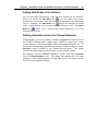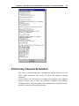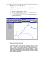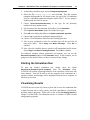
1
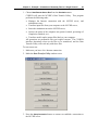
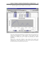
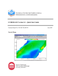
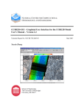
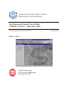
NATIONAL CENTER FOR COMPUTATIONAL HYDROSCIENCE AND ENGINEERING One-Dimensional Channel Network Model CCHE1D Version 3.0 – Quick Start Guide Technical Report No. NCCHE-TR-2002-03 Dalmo A. Vieira School of Engineering The University of Mississippi University, MS 38677 January 2002 NATIONAL CENTER FOR COMPUTATIONAL HYDROSCIENCE AND ENGINEERING Technical Report No. NCCHE-TR-2002-03 One-Dimensional Channel Network Model CCHE1D Version 3.0 – Quick Start Guide Dalmo A. Vieira Research Associate Revision Number: 27 The University of Mississippi January 2002 Contents CHAPTER 1 Introduction 1 Purpose 1 Applicability Statement 2 How to Use This Document 2 Required Engineering Expertise 2 Related Documents 3 Technical Support and Training 3 CHAPTER 2 Starting CCHE1D 4 Introduction 4 To Create a New CCHE1D Project 4 To Open an Existing CCHE1D Project 6 Final Notes 7 CHAPTER 3 Example 1: Simulation of Unsteady Flow in a Single Channel 8 Introduction 8 Contents ii Case Description 8 Input Data 9 Creating a New Test Case 9 The Project File Creating the Simulation Domain 9 10 Digitizing a Channel Network 10 Importing a Background Image 11 Digitizing the Channel Planform 13 Creating the Computational Network 18 Adding Computational Nodes 18 Adjusting Channel Reach Lengths 20 Supplying Cross Section Data 20 Refining the Channel Network 21 Performing Channel Simulation 21 Defining Model Output 21 Defining Run Parameters and Options 24 Executing the Channel Simulation 25 Visualizing Results 27 CHAPTER 4 Example 2: Simulation of Flow and Sediment Transport in a Channel Network 30 Introduction 30 Case Description 30 Input Data 31 Creating a New Test Case 31 Creating the Simulation Domain 32 Extracting a Channel Network from a DEM 32 Importing the DEM 32 Pre-Processing the DEM 34 Contents iii Extracting the Channel Network 35 Creating the Computational Network 40 Adding Cross Section Data 41 Adding Hydraulic Structures to the Channel Network 44 Refining the Computational Network 45 Performing Channel Simulation 47 Displaying Node Numbers 48 Defining Model Output 48 Creating a Chart List 49 Specifying Simulation Parameters and Boundary Conditions 50 Starting the Simulation Run 51 Visualizing Results 51 Final Words 52 CHAPTER 1 Introduction Purpose This Quick Start Guide is intended to help new users become familiar with CCHE1D by providing step-by-step instructions for example applications that demonstrate the use of the modeling components and auxiliary tools. This manual adopts a “hands-on” approach, where you learn by following examples, instead of combing through the thick User’s and Technical Manuals. This guide gives emphasis to the use of the software through the ArcView graphical interface, especially to the process of data preparation. Two main examples are described in this guide, which demonstrate how CCHE1D can be used to model practical engineering problems. This guide does not show all the capabilities of the CCHE1D software, nor it describes in detail the functionality of each tool or feature. For a complete description of the programs, data structures, etc., please consult the CCHE1D User’s Manual. In addition, before using the CCHE1D model, you should have a good understanding of the assumptions and methodologies employed in the model. For detailed information on the theoretical background of the models, implementation procedures, program structure, etc., please refer to the CCHE1D Technical manual and publications listed in the References sections of the User’s and Technical Manuals, as well as publications listed in the CCHE1D website, at http://www.ncche.olemiss.edu/cche1d. Chapter 1 Introduction 2 Applicability Statement This guide applies to CCHE1D version 3.0. It updates and supersedes any previous version of this manual. CCHE1D 3.0 requires ArcView GIS version 3.0a ~ 3.3. Please install update patches for ArcView 3.x, available from the Environmental Systems Research Institute, at http://www.esri.com/. CCHE1D does not work with ArcView 8.x or 9.x. How to Use This Document This guide assumes CCHE1D is already installed and working correctly on your computer. If you have problems with software installation, consult the CCHE1D User’s Manual, or contact the program developers for help. This guide uses data sets of real watersheds in the United States to illustrate how the model can be used in the simulation of channel flow and sediment transport. In the first example, GIS data layers are employed to describe a reach of the East Fork River, in Wyoming. All the necessary are included with the CCHE1D software. Another example uses the Goodwin Creek Watershed, in Mississippi, to illustrate a combined watershed–channel network simulation, in which simulation data from the SWAT watershed model are used as boundary conditions for the simulation of flow and sediment transport in a network of channels. These examples should be enough to give a new user a good understanding of the modeling approach adopted by CCHE1D, as well as to demonstrate its main features and capabilities. By following the examples of this guide, you should be able to “operate” CCHE1D. You should then proceed to the CCHE1D User’s Manual for more detailed explanations for each step of the simulation process. Finally, you should review the Technical Manual to be able to model channel flow and sediment transport problems correctly. Required Engineering Expertise The use of CCHE1D requires a certain level of expertise from the part of the user. In fact, the user of this program is the real “modeler” who must describe a physical domain in such a way that a numerical solution of the flow and sediment transport equations is stable and accurate. Before applying the model to the study of any flood and/or transport study, one must read the CCHE1D Technical Manual carefully to understand how CCHE1D models the physical phenomena, and especially to become familiar with the assumptions and limitations that are present in the model. Although the CCHE1D model has been considerably improved in order to handle a large variety of flow conditions that typically occur in nature, there could be Chapter 1 Introduction 3 situations where the underlying hypotheses of the model were not satisfied, and the model could yield inaccurate or even erroneous results. It is responsibility of the user to employ this sophisticated tool in a reasonable, scientifically sound way. The CCHE1D interface certainly facilitates the use of the model, but engineering sense is still required. Related Documents The documentation of CCHE1D is separated into several publications designed to fulfill the needs of different audiences. The present document, the “CCHE1D Quick Start Guide”, is intended primarily to users who will use CCHE1D for the first time, and therefore are not familiar with program. For detailed instructions on how to use CCHE1D, and for documentation on input files, etc., read the report “One-Dimensional Channel Network Model CCHE1D – Technical Manual.” For a more technical discussion of the CCHE1D Channel Network Model, and for guidance on the modeling of flow and sediment transport in channels, please consult the “One-Dimensional Channel Network Model CCHE1D – Technical Manual.” In addition, the CCHE1D web site (http://www.ncche.olemiss.edu/cche1d) lists a series of publications that discuss the development, testing, and application of the model. Technical Support and Training The model development staff is available to answer any questions concerning the software and its application in the modeling of engineering problems. If you have any questions, or need more information about model capabilities and limitations, model assumptions, methods, and techniques, or any other technical issue, please feel free to contact the NCCHE. Consult the NCCHE web site for current contact information. There is no charge for this service. The NCCHE may be able to arrange training sessions or technical consulting tailored to your particular type of problem or application. If the current version of CCHE1D does not offer a particular feature or capability required for your intended application, arrangements can be made to enhance the current software, depending on the model’s development time-table, and provided a cost-sharing agreement can be reached. CHAPTER 2 Starting CCHE1D Introduction This section describes the basic procedures for starting CCHE1D and creating a new test case. For version 3.0, however, a new automated system has been implemented, which allows CCHE1D to be started as any Windows program. Look for CCHE1D in the Windows Start button, or click on the CCHE1D icon on your desktop, if it is available. For general information on creating CCHE1D test cases, understanding CCHE1D/ArcView projects, managing data files, etc., please read the sections near the end of “Chapter 3 – Installing and Starting CCHE1D” of the User’s Manual for important information. For now, the basic information to start CCHE1D is given here below. To Create a New CCHE1D Project To start CCHE1D to create a new test case, you can start CCHE1D like any other windows program: 1. Double-click on the CCHE1D icon on your Windows desktop. If you do not see the icon, use the Start Menu as usual for any Windows program. CCHE1D is the Programs/NCCHE group. On newer versions of Windows, the CCHE1D icon is also available from the task bar, usually at the bottom of the desktop. 2. You will see ArcView starting, and then the CCHE1D banner is displayed. A new dialog appears. Choose Create a new case and press OK. Chapter 2 Starting CCHE1D 5 3. You will then be prompted to enter a “Project Case Name.” You can navigate your computer and define a location for the new CCHE1D project using the right-hand side panel of the dialog. Otherwise, simply provide a case name but limit it to eight characters, and do not use spaces or special symbols (< , . ? ( [ }& \ / * ). If you prefer to start ArcView first, or if you already have ArcView running, you can start CCHE1D by enabling its Extension: 1. In ArcView’s File menu, select Extensions. You must have ArcView’s main window (the “Project” window) active to see this option. 2. Scroll down the list of extensions available on your computer, and select CCHE1D. A black checkmark appears. Press the OK button. If you cannot see the CCHE1D extension in the list, the software was not installed correctly. Make sure the extension file cche1d-3.avx is installed in the proper directory. Chapter 2 Starting CCHE1D 6 3. If there is already an open ArcView project, the CCHE1D banner is displayed, and you are prompted to enter a “Project Case Name.” You can navigate your computer and define a location for the new CCHE1D project, if desired. Otherwise, simply provide a short case name (not more than eight characters) and press OK. 4. If there is no open project, use the New Project option of the File menu. The CCHE1D banner is displayed, and you are prompted to enter a “Project Case Name.” You can navigate your computer and define a location for the new CCHE1D project, if desired. Otherwise, simply provide a short case name (not more than eight characters) and press OK. 5. Save the new ArcView project, as usual. To Open an Existing CCHE1D Project There are three different ways of opening an existing CCHE1D-ArcView project. 1. You can open an existing CCHE1D project simply by double-clicking the ArcView Project file icon. The ArcView file has extension .apr and is located inside the folder with the same name (without the extension). On Windows systems, the icon also appears in the “Documents” or “Recent Documents” part of the Windows Start menu. 2. Alternatively, you can start ArcView and then use the Open Project option of the File menu. Chapter 2 Starting CCHE1D 7 3. You can start CCHE1D directly, using the CCHE1D 3.0 icon on your desktop on in the Windows Start menu. Choose Open existing case in the dialog that follows. Final Notes CCHE1D cannot work unless you provide the case name. If you cancel the creation of the test case, the project is closed, but the extension remains active. Simply use the “New Project” option to create a new CCHE1D Project. Once a case name is defined, CCHE1D creates a directory with the same Case Name at specified location. It is very important to always save the ArcView project. If you are already familiar with ArcView you know that ArcView project files (extension .apr) do not store the data such as tables, graphics, etc., but only references to other files in the computer system. If you forget to save the project file, references to the files may be lost. Read the instructions and usage guidelines of the User’s Manual, especially Chapter 3, where important tips are given for the general use of CCHE1D. If you are not familiar with ArcView, it is recommended that you spend one hour or so familiarizing yourself with that program to understand how it works. CHAPTER 3 Example 1: Simulation of Unsteady Flow in a Single Channel Introduction This chapter will use data for the East Fork River, in Wyoming, USA, to illustrate how CCHE1D can be used to simulate unsteady flow in a natural river. In this example, you will define simulation domain using GIS data and the Channel Network Digitizing module. You will prepare the computational mesh, define the model output, and simulate continuous flow for a period of approximately 30 days. Case Description The East Fork River was an experimental river for the study of bed load transport in the 1970’s. The study reach is 3.3 km in length and terminates downstream at a bed load trap constructed across the river. The drainage area of the East Fork River at the bed load trap is about 500 km2. During the spring runoff, diurnal fluctuations due to snowmelt are characterized by a rising stage during the morning, a peak stage at midday, and a falling stage during the afternoon. In this example, CCHE1D will be used to simulate continuous flow for about 30 days, for which measured data are available. Chapter 3 Example 1: Simulation of Unsteady Flow in a Single Channel 9 Input Data All required data files for this exercise are part of the CCHE1D distribution. Data files used in this chapter are located in the folder <drive letter>:\ncche\cche1d-3\tutorial\efr, assuming CCHE1D has been installed in the default location. If you are asked to open or import a certain file, make sure to use the “file open” dialog to navigate to that location. Alternatively, you may want to copy the contents of that folder to another location of your preference. For simplicity, the data folders used in this manual will be simply referred as, for example, tutorial\efr instead of the full path name as given above. GIS data layers used in this exercise were obtained from the Wyoming Spatial Data Clearinghouse (http://wgiac.state.wy.us/wsdc). Creating a New Test Case In order to start working with CCHE1D, let us start the CCHE1D ArcView interface and create a new test case for the East Fork River data. 1. Start CCHE1D. Either click on “CCHE1D 3.0” in the Windows Start Menu, or click on the CCHE1D 3.0 icon on your desktop or task bar. 2. A dialog will appear, asking for a “Case Name.” Enter a short alphanumeric name, like efr1, but limit it to eight characters, and do not use spaces or special symbols (< , . ? ( [ }& \ / * ). Note that the simulation data will be written to the location shown in that dialog. You can navigate to another folder, if you like it. Chapter 3 of the User’s Manual discusses how you can define the default location for your CCHE1D cases. 3. Press OK when done. Note that a new folder, with the same name you gave to the Test Case, was created at the specified location. All data files created by CCHE1D will be stored inside that folder. The Project File Inside the recently created folder, there is a file with the same Case name but with extension .apr. This file is the ArcView Project File. It stores the current state of your CCHE1D project. To open an existing case, simply double-click on the .apr file. The project file does not store the data elements for the maps, tables, model input and output, etc, but only references to other files present in your computer. Chapter 3 Example 1: Simulation of Unsteady Flow in a Single Channel 10 Creating the Simulation Domain Digitizing a Channel Network Now we are going to create a computational mesh for the simulation of the 3.3-km reach of the East Fork River. We are going to use the Channel Network Digitizing module of CCHE1D, in which you will “draw” the channel by following what you see in an aerial photograph. To start the Channel Digitizing Module, follow these steps: 1. Choose the option Digitize Channel Network, from the Channel-Network menu. 2. In the dialog that follows, choose Yes to import a Background Theme, and continue to the next section. Chapter 3 Example 1: Simulation of Unsteady Flow in a Single Channel 11 Importing a Background Image When you decide to import a background theme, you are asked to specify what kind of GIS data you are going to use as reference. It can be an Image (a photograph, scanned map, etc), a Feature theme (ArcView Shapefiles), a Grid theme (ArcView or ArcInfo raster grids), or a CAD file. If you are not continuing from the previous section, choose Import Background from the Channel-Network menu. Continue with the following steps: 3. Choose Image in the dialog that appears. 4. In the dialog that follows you are asked if you want to activate a different ArcView Extension (an add-on) to enable support for a specific data type. Answer Yes, because we are going to use an image in the Mr.Sid format, which is requires the activation of an specialized Extension. Chapter 3 Example 1: Simulation of Unsteady Flow in a Single Channel 12 5. In the dialog that follows, click on “Mr. Sid Image Support.” Make sure you have a black check mark by the extension name. Press OK to continue. 6. In the dialog that follows, select the background image file. Make sure you have “Image Data Source” in the Data Source Types field at the bottom-left corner of the dialog. Select the proper drive letter where you have CCHE1D installed (usually C:\), and then go to the folder NCCHE\CCHE1D-3\tutorial\efr. You should see the file efr_photo.sid at the left panel of the dialog. Double-click to select and import that file. 7. In the dialog that follows, you will be asked if you want to start digitizing a channel network. Answer No. Chapter 3 Example 1: Simulation of Unsteady Flow in a Single Channel 13 8. Make the theme visible by clicking on the small square on its legend, to the left of the image area. By now, you should see a new window, entitled “Channel Network Digitizing View 1.” In this window, you will digitize the channel(s) visible on your reference theme, in this case, a Digital Orthophoto converted to the MrSid file format. You can use the zoom and pan tools to see the detail of the image. About the Coordinate System The photograph you imported was already referenced to a known coordinate system. That is why you can see real coordinate values at the top-right corner of the CCHE1D interface. If you intend to use an image that is not already referenced to a known coordinate system, you can use the CCHE1D Image Georeference Extension, which allows you to provide the necessary data for establishing the relationship between features in the image and points of known coordinates. Once the image is georeferenced, CCHE1D can use real distances when creating the input data for the model. If the image is not referenced, all coordinates will be approximately between 0.0 and 1.0. Digitizing the Channel Planform Having the Channel Network Digitizing View ready with the reference image, we must now locate the region of interest. Maximize the image size and zoom-in at the East Fork River, near the northeast corner of the image. Use the picture below as reference. Another Reference Layer Because you are not familiar with this particular river reach, we are going to give you the exact location of the cross section survey points in the simulation domain. Suppose a surveyor used a GPS system to locate these particular points, and you know the coordinates of these points. We are going to import the data into CCHE1D, and you will have a visual reference to start digitizing the channel reach of interest. This step is not really necessary, but it is included here to demonstrate the power and versatility of GIS techniques. 1. Having the Channel Network Digitizing View active, choose Import Background from the Channel-Network menu. 2. Select Feature (shapefile) in the dialog that appears. 3. Go to the folder tutorial\efr, and select the file efr_cs_loc.shp. Make sure “Data Source Types” is set to “Feature Data Source,” or you will not see the file. 4. You can change the order of the layers by moving the bar with the layer name, in the legend area, to the left of the image, in the Channel Network Digitizing View. Chapter 3 Example 1: Simulation of Unsteady Flow in a Single Channel 14 A data file as the one you just imported can be created in minutes if you have the point coordinates, using standard ArcView functionality. Search the ArcView on-line manual for Event Theme Tables to learn how to create such map layer. A Rough Sketch On-screen digitizing requires a bit of practice, and sometimes, a good deal of patience. However, using the available editing tools, you can start from a rough sketch and then refine the channel network, so that the final result satisfies your requirements for accuracy. If you do not have a reference to a real-world coordinate system, maybe the simple sketch will suffice. There are a few rules you must follow when creating channel data using the channel digitizing interface. They are discussed in details in the user manual. For this example, the rules that must be obeyed are: 1. The main channel line must be continuous; 2. It should be drawn in the direction of flow (from upstream to downstream). Chapter 3 Example 1: Simulation of Unsteady Flow in a Single Channel 15 For the East Fork River simulation, a single channel will be created, therefore, there should be only one continuous line describing the channel. If this is the first time you work with ArcView and CCHE1D, you may have to repeat steps 3 and 4 to gain some practice with the channel digitizing tool. When digitizing, do not worry about getting every bend of the river accurately. Just add a number of points to get the general shape of the channel. You may edit it to add detail later. 1. With the Channel Network Digitizing View active, choose New Channel Network from the Channel-Network menu. A new empty theme named Digitized Channels appears. Note: If you had already created the Digitized Channels theme, you can start editing using Start Editing Network from the Channel-Network menu. If you want to discard the digitized channels, use the option Delete Channel Network. 2. Maximize the Channel Network Digitizing View and use the “Pan” and “Zoom” tools to have the entire simulation reach visible on screen. 3. Make sure the Digitized Channels theme is active, and that the “Digitize Channel” tool is selected. Chapter 3 Example 1: Simulation of Unsteady Flow in a Single Channel 16 4. The East Fork River flows from south to north. Click at the upstream point, and then move the mouse over the river visible in the background photograph. Click the left button to add points along the river, defining its contour. Do not stop until you reach the end. 5. When the end point is reached, double click the left button to terminate the line. 6. Choose Stop Editing Network from the Channel-Network menu. The main issue here is to have a single continuous line defining the river contour. For now, if you accidentally stop before the end point, delete the channel line and start over. It is possible, however, to edit channel lines, see the User’s Manual for more information. To delete a digitized line: 1. Activate the “Pointer” tool . 2. Select the line and press the Delete key. To quickly verify you have a single line describing the channel, use the “Open Theme Table” tool to open the attribute table corresponding to the Digitized Channels theme. You should see a single line, with the word “Polyline” at the first column. Adding Details If the channel lengths are going to be inferred directly from your digitized channels, it pays to edit the digitized lines so that they represent features like bends and meanders accurately. Keep in mind that CCHE1D is a onedimensional model, and therefore, a realistic channel planform may not be necessary, provided you specify accurate channel lengths (from a survey, for example) using the editing tools of the interface. In this example, accurate channel reach lengths will be given as part of the cross section geometry data, and this section is for demonstration purposes only. Therefore, inaccuracies in the channel digitizing will not hinder the quality of the simulation. To edit an existing digitized channel: 1. Start editing the Digitized Channels theme. Make the Channel Network Digitizing View active; choose Start Editing Network from the ChannelNetwork menu. 2. Use the “Zoom” and “Pan” to edit. 3. Select the “Vertex Edit” tool . tools to zoom-in to the area you want 4. Click on the channel line. Each point that defines its shape is marked with a square. Chapter 3 Example 1: Simulation of Unsteady Flow in a Single Channel 17 5. To move a point: a. Move the mouse over the point you want to move. The cursor should change to a “plus” sign. b. Click and hold the left button. Move the point and release the button at the new location. 6. To add a point: a. Move the mouse over the channel line at the location you want to add a point. The cursor should change to a “encircled plus” sign. b. Click to add a new point. 7. To delete a point: a. Move the mouse over the point you want to move. The cursor should change to a “plus” sign. b. Press the Delete key to remove the point. c. To “undo” the deletion, press CTRL-Z, or choose Undo Feature Edit from the Edit menu. 8. You can zoom and pan without deactivating the “Vertex Edit” tool by clicking the right-clicking on the map to bring a pop-up menu. Chapter 3 Example 1: Simulation of Unsteady Flow in a Single Channel 18 9. Use Stop Editing Network in the Channel-Network menu. Save the changes. 10. Choose Validate Channel Network in the Channel-Network menu to make CCHE1D inspect the digitized channel network. Informational messages will be displayed indicating whether the channel network is valid (correct) or not. Creating the Computational Network Once you have completed the channel digitizing, you may proceed to create the computational channel network, that is, define how the simulation domain will be discretized into nodes and elements for the Finite Difference simulations of flow and sediment transport. To create a Computational Network based on a digitized channel network, simply: 1. Make the Channel Network Digitizing View active; choose Create Computational Network from the Channel-Network menu. A new window appears, named Channel Network 1. Note that when the new window is active, the menus, buttons, and tools change, showing new options and tools. From now on, you will work only on this window. You can close the Channel Network Digitizing View. To open it again, select it from the Channels group of the Project window. Adding Computational Nodes The first task will be defining the computational grid for the simulations. Grid generation is the most time consuming task of the simulation procedure. It requires engineering expertise and understanding of numerical techniques. CCHE1D provides a series of tools that help with tedious tasks of data preparation, but it does not replace knowledge and experience in numerical modeling. Keep in mind that if the numerical grid is inadequate, the model may produce inaccurate results, or may not even converge to a solution. We will define the same number of cross sections that are available from a field survey, or 41 nodes. The exact relative position for each node is given together with the cross section geometry, in the file eastfork.cs. The channel network already contains two nodes, a Source node at the upstream end, and the Watershed Outlet node at the other end. We must now add the remaining 39 nodes. For that, we will make use of a sketch produced by the surveyors, which was scanned and georeferenced to the same coordinate system of the aerial photograph used as reference. Let us add the reference layer: Chapter 3 Example 1: Simulation of Unsteady Flow in a Single Channel 1. Make the Channel Network 1 active, and Import Background from the Channel-Network menu. 2. In the dialog that appears, select Feature (Shapefile). use the 19 option 3. Browse your computer and select the file efr_cs_loc.shp in the tutorial\efr folder. Now, we will add computational nodes at survey locations: 1. Make the Channel Network 1 window active, and zoom-in so that the first five or so cross section locations fill the map window. . Click on the channel line, at the position 2. Select the “Add Node” tool of each cross section, to add nodes. Use the “Pan” tool to make other . nodes visible, and then reactivate the “Add Node” tool 3. Repeat until the 39 interior nodes are added. Do not add extra nodes yet, because the cross section file supplied for this example matches the nodes of the diagram. 4. When finished, delete the background by selecting Delete Background from the Channel-Network menu. Select the theme (efr_cs_loc.shp) from the list that appears, and press OK. Chapter 3 Example 1: Simulation of Unsteady Flow in a Single Channel 20 Adjusting Channel Reach Lengths At this stage, you could edit the length of each channel reach (segment between nodes) to correct errors due to distortions in the photograph and inaccuracies inherent to the digitizing and graphical editing. In this example, however, the cross section geometry data contains the distances along the channel between consecutive survey points. Therefore, it is not necessary to edit them manually. Strictly speaking, even the position of the nodes added in the previous section could be disregarded. You could have the mesh as a simple sketch, having all nodes equally spaced within the domain, because the real distances are given inside the cross section geometry file. Furthermore, when you adjust channel reach lengths, the channel network map is not modified. If you add a node to a reach with an user-defined length, the new lengths will be compute ed using the relative position of the new node and the user-defined reach length. Consult the CCHE1D User’s Manual for other mesh editing capabilities. Supplying Cross Section Data Now that the basic channel network has been defined, we must provide the channel geometry for the computational nodes. For the simulation, channel geometry must be defined at each node. However, in practical cases, data are rarely available at this level of detail. CCHE1D requires known geometry only at the beginning and end of channels, and it can use linear interpolation to generate data for nodes without data. Of course, providing data for only two points would be a crude approximation. The cross section geometry file provided for this example contains real survey data for all nodes. The data also includes values Manning’s roughness coefficient n. To import the cross section data: 1. With the Channel Network 1 active, select Import from the Cross Section menu. 2. Select Geometry in the dialog that follows, then press OK to continue. 3. Press OK to confirm that input file reference locations “by node numbers.” 4. Select the file Eastfork.cs, in the tutorial\efr folder. After a couple of seconds, while CCHE1D updates its database, a message will be displayed indicating the operation was successful. Chapter 3 Example 1: Simulation of Unsteady Flow in a Single Channel 21 Refining the Channel Network After the available cross section data are imported, you can refine the computational mesh to improve the quality of the numerical simulations. You , “Add Nodes” , or “Remove Node” tools. can use the “Add Node” If you add a node, CCHE1D will utilize the nearest supplied cross section data to generate interpolated geometry for the new node. In this example, only flow simulations will be performed. Therefore, there is no sediment related data to be supplied, and the channel network is practically ready for the simulations. Performing Channel Simulation Defining Model Output CCHE1D does not have a “standard” output file, because there are many combinations that can be used for output. The user has the flexibility of Chapter 3 Example 1: Simulation of Unsteady Flow in a Single Channel 22 choosing which variables should be output, at what locations (nodes), and at which frequencies. You can interpret the specification of model output for CCHE1D as defining what charts you would like to see when the simulation is complete. For that, you create the so-called “Chart Lists.” For example, you can define you want time series for water discharge and water level at given locations, but with different frequencies for each location. You can decide you want a water surface profile along a certain segment, etc. Output results are given for Nodes. Use the Show Node Numbers option in the Channel-Network menu to display node numbers on the channel network view. We are going to ask CCHE1D to prepare data for 2 charts. CCHE1D itself does not create the plots, but it prepares the data so you can use import it into your favorite plotting package, such as Microsoft Excel, Tecplot, or any program with x-y plotting capability. 1. Choose Create Chart List from the Simulation menu. A new theme, named Chart Definition 1 is added to the view. 2. The tool “Add Node to Chart List” should be automatically selected. This tool allows you to define a chart for a particular node. Click on a Chapter 3 Example 1: Simulation of Unsteady Flow in a Single Channel 23 node to select it, for example, node 40, one upstream of the watershed outlet. 3. Select Nodal Time Series as data type, in the dialog that follows. 4. Enter a frequency, in number of time steps. Let us say 100 for now, we can edit it later. 5. Select the tool “Add Profile to Chart List” so that we can define a profile along the channel. Click on a node at or near the upstream end, let us say node 5 and 35. It should be highlighted in light blue. Click on a node at or near the downstream end of the channel. Provide a frequency for output; let us say 300 time steps. The determination of which values that will be output for each type of plot will be done in the next section. You can double-click on the legend of the Chart Definition theme to choose a different classification for that theme. Chapter 3 Example 1: Simulation of Unsteady Flow in a Single Channel 24 Defining Run Parameters and Options All run parameters and options are specified through a series of dialogs that are displayed in sequence. Please consult the User’s Manual for detailed explanations of their meaning. For now, supply the values when asked according to the table given below. Use the Tab key to change fields within the dialog, and press the Enter key or the OK button to proceed to the next. 1. Select General Parameters from the Simulation menu. small dialogs will be displayed. 2. Provide the values according to the table below: A sequence of Dialog number Description Value 1 Number of Storm Events to 1 Simulate 5 Time Step Size, in minutes 2 Type for Boundary Conditions Time-discharge hydrographs File 3 Select the upstream boundary tutorial/efr/eastfork.bc conditions file 4 Type of Downstream Boundary User-specified stage time-series Condition 5 Select the downstream tutorial/efr/eastfork.by boundary conditions file 6 Method for Determination of User-specified discharges Baseflow 7 Select the baseflow file tutorial/efr/eastfork.bf 8 Select the Flow Modeling Type Dynamic Wave Model Chapter 3 Example 1: Simulation of Unsteady Flow in a Single Channel 25 Treatment Disable small depth algorithm 9 Small Depth Algorithm 10 Select a Chart Definition Table 11 Select Variables for Time Series Select Water Discharge and Stage. Press and hold the SHIFT key for Output multiple selections. 12 Select Variables for Profile Select Stage. Output Chart Definition 1 Executing the Channel Simulation Once the General Parameters are set, you can start the CCHE1D channel flow model for the simulation. A simulation can be executed on the same computer the interface is running (the preferred option), or on the NCCHE server, which is available free of charge. Running the model on the local computer 1. Choose Start Channel Simulation (Local Computer) from the Simulation menu. CCHE1D will perform a series of checks on its database, which may take several minutes, if there are many recent changes to the mesh or cross section data. After the initial checking is complete, the interface will transfer all the data to the simulation module. A series of informational messages are displayed. Each time a simulation is started, a new “run number” is assigned. This way, results from a previous simulation are not overwritten, and remain on your computer hard disk. Although the interface attempts to detect errors in the input files, some problems in the input data may be detected only when the simulation takes place. Error messages issued by the model are also displayed on the graphical interface. The following section shows how to access the simulation results. Running the model on the NCCHE Server (optional) NCCHE provides a computer server free of charge for registered users. To use the server, please contact NCCHE for an account and password. Internet access is required. Chapter 3 Example 1: Simulation of Unsteady Flow in a Single Channel 26 1. Choose Start Remote Server Run from the Simulation menu. CCHE1D will start the NCCHE’s Data Transfer Utility. This program performs the following tasks: Manages the Internet connection with the NCCHE server, and authenticates user; Transfers input files from your computer to the NCCHE server; Starts the simulation run on the NCCHE server; Queries the status of the computer run (queued, started, percentage of completion, finished, etc.); Transfers model results (output files) back to your computer. All operations are performed with your explicit consent. The CCHE1D interface determines what are the files to be transferred, and the Data Transfer Utility will work only with these files. To start a new run: 1. Make sure you have a live Internet connection. 2. Make the Data Transfer Utility window active. 3. Press the Setup Connection button to connect to establish a connection to the NCCHE server. Chapter 3 Example 1: Simulation of Unsteady Flow in a Single Channel 27 4. Provide your Username and Password in the dialog that follows. Make sure “Remote NCCHE Server” is selected. Users within the NCCHE computer network should use the option “Local NCCHE Server.” 5. Use the Upload Files button to transfer the input files to the NCCHE server. When data transfer is finished, use the Start New Simulation button to start the simulation. After the remote simulation starts, you can close the Data Transfer Utility, the CCHE1D interface, and your connection to the Internet. You can check the status of the run at any time, by opening the Data Transfer Utility using the Start Data Transfer Utility option in the Simulation menu. Do not use the Start Remote Server Run option to check on an existing run. Use the Check Progress button to get the current status of the simulation run. When the simulation is complete, you can request that the simulation results be transferred back to your computer. Use the Download Files button to retrieve the output data. After you verify the simulation results are safe on your computer, you should delete all data files present on the NCCHE server, by pressing the Remove Files from Server button. Storage space is limited, and it is shared by all CCHE1D. As an act of courtesy, please remove the data files from the NCCHE server as soon as possible. Visualizing Results Simulation results are always stored inside the simul folder, in the current case folder, which is displayed at the top of the main window. Output files are named according to the following convention: Time Series Charts: <casename>_mp_run<Number>_ts-<NodeNumber>.txt Profile Charts: <casename>_mp_run<Number>_prf-<NodeNumberUS><NodeNumberDS>.txt Cross Section Geometry Charts: <casename>_mp_run<Number>_cs-<NodeNumber>.txt Sediment Size Class Data Charts: <casename>_mp_run<Number>_sz-<NodeNumber>.txt All file are text files, and can be opened and edited with any text editor, such as Notepad, Wordpad, or text processors like Word and WordPerfect. These files can be imported directly into many electronic spreadsheet, plotting, and visualization programs. Chapter 3 Example 1: Simulation of Unsteady Flow in a Single Channel 28 As an example, we are going to show how to open this file into the electronic spreadsheet program Microsoft Excel, and plot time-series results. 1. In Microsoft Windows, use the Windows Explorer to browse your computer to the simul folder where the results are stored. 2. Locate the Time Series data file (named efr1_mp_run1_ts-40.txt if you used the suggested names and node numbers). 3. Click with the right mouse button, and choose the “Open With…” option. On Windows 95/98/NT, you may have to press the SHIFT key for this option to appear in the menu. Choose Microsoft Excel from the list that appears. Excel should open, displaying the contents of the data file. 4. Alternatively, if you have Excel already running, you can simply Open the output file (select Text Files as file type in the Excel dialog). Excel should display the “Text Import Wizard.” Choose “Delimited” in the first panel. Click “Next.” Make sure “Tab” is select as the delimiter, in the next panel. Click “Finish” to complete importing the file. 5. Once the file is open, you should see a single numeric value in each Excel cell. If all contents appear in the first column of the spreadsheet, try importing the file again. You can now select data to plot and use Excel charting options to quickly create your time series plots. 1. Select columns “Sim_Time” and “Discharge” by clicking on the labels at the top (hold the CTRL key to select the second column). 2. Click on the Chart Wizard icon, in the Excel toolbar, or choose Chart from Excel’s Insert menu. 3. In the dialog that follows, select “XY (Scatter) as chart type. Choose a subtype and click “Next.” Chapter 3 Example 1: Simulation of Unsteady Flow in a Single Channel 29 4. Edit chart options or press “Finish” to see your chart. This short example demonstrated how to quickly prepare the input data for an unsteady flow simulation in a single channel. It also showed the basic procedures for defining the type of output and performing the channel simulations. Please refer to the User’s Manual to learn about all the options and capabilities the CCHE1D software has to offer, and to learn how to prepare the data files that were provided for this exercise. CHAPTER 4 Example 2: Simulation of Flow and Sediment Transport in a Channel Network Introduction This chapter will teach you how to perform a simple channel flow analysis for a complete watershed analysis using CCHE1D. You will simulate the runoff and sediment transport through the Goodwin Creek watershed in northern Mississippi, using simulation results obtained with the watershed model SWAT. In this exercise, you will create a channel network using the methods of “Landscape Analysis,” where the drainage network is inferred from elevation data from a Digital Elevation Model (DEM). You will then create the computational channel network, and add channel geometry, hydraulic structure, and sediment-related data. Case Description The Goodwin Creek Experimental Watershed was established in 1977 to serve as a prototype of the much larger Demonstration Erosion Control Project (DEC) watersheds. The drainage area above the watershed outlet is 21.3 km2. Terrain elevation ranges from 71m to 128m above mean sea level, producing an average channel slope of 0.004. Most of the channels in the watershed are ephemeral, with perennial flows occurring only in the lower reaches of the Chapter 4 Simulation of Flow and Sediment Transport in a Channel Network 31 watershed. The runoff produced by storm events swiftly exits the watershed, and the discharge returns to baseflow levels within one to three days. The sediment transported in the channels ranges from silt (< 0.062mm) to sand to gravel (< 65mm). The watershed is partitioned into 14 nested subbasins by the in-stream gauging structures that were built to control channel degradation and to measure discharges, stages, and sediment yield. A computer-based acquisition system collects and transmits data from the gauging stations to the USDA-ARS National Sedimentation Laboratory, in Oxford, MS, which is responsible for the monitoring program. Periodic channel surveys, bed and bank sediment sampling, a rain gauge network, and a detailed inventory of upland soil types and land use complement a dataset that provides an excellent means to verify upland and channel flow and sediment transport models Input Data All required data files for this exercise are part of the CCHE1D distribution. Data files used in this chapter are located in the folder <drive letter>:\ncche\cche1d-3\tutorial\goodwin, which from now on is referred simply as tutorial\goodwin. If you are asked to open or import a certain file, make sure to use the “file open” dialog to navigate to that location. Alternatively, you may want to copy the contents of that folder to another location of your preference. All input data used in this exercise were prepared by or obtained through the USDA/ARS–National Sedimentation Laboratory, in Oxford, MS, which is responsible for monitoring the Goodwin Creek Watershed, and was actively involved in cooperative research for the development and application of modeling tools as part of the Demonstration Erosion Control Project. Watershed modeling work using SWAT was performed and provided by Dr. Ronald L. Bingner, of that institution. Creating a New Test Case In order to start working with CCHE1D, let us start the CCHE1D ArcView interface and create a new test case for the East Fork River data. 1. Start CCHE1D. Either click on “CCHE1D 3.0” in the Windows Start Menu, or click on the CCHE1D 3.0 icon on your desktop or task bar. 2. A dialog will appear, asking for a “Case Name.” Enter a short alphanumeric name, like gcw1, but limit it to eight characters, and do not use spaces or special symbols (< , . ? ( [ }& \ / * ). Note that the simulation data will be written to the location shown in that dialog. You can navigate to another folder, if you like it. Chapter 3 of the User’s Chapter 4 Simulation of Flow and Sediment Transport in a Channel Network 32 Manual discusses how you can define the default location for your CCHE1D cases. 3. Press OK when done. Note that a new folder, with the same name you gave to the Test Case, was created at the specified location. All data files created by CCHE1D will be stored inside that folder. You can save your project at any time by selecting the Save option from the File menu, or by clicking the button. Creating the Simulation Domain Extracting a Channel Network from a DEM In this example, we are going to create a channel network using an automated procedure referred to as “Landscape Analysis,” in which a program called TOPAZ – TOpographic PArameteriZation, is used to analyze elevation data and define the drainage network and delineate the drainage basin. Please refer to the CCHE1D User’s Manual for a detailed discussion on the methods and on the several options CCHE1D offers. Importing the DEM We start by importing a DEM file, from which a channel network will be extracted. A DEM stores elevations as “raster data,” that is, a matrix of equally spaced points with known elevations. 1. Select the Import DEM option from the Channel-Network menu. 2. CCHE1D supports different DEM formats. For this exercise, select ArcInfo ASCII file. Chapter 4 Simulation of Flow and Sediment Transport in a Channel Network 33 3. In the window that appears, navigate to the location of the tutorial\goodwin directory. 4. Select the file Goodwin_arc.dem and press OK. CCHE1D will read the file and create a view of the DEM. The window is named Raw DEM 1. Chapter 4 Simulation of Flow and Sediment Transport in a Channel Network 34 Pre-Processing the DEM Now that you have imported the DEM, the next step in the analysis is to fix some possible deficiencies of the original DEM, to ensure that the analysis algorithms of TOPAZ can extract a complete channel network for this DEM. Follow the steps below to pre-process the DEM: 1. Select Preprocess from the DEM menu. 2. In the dialogs that follow, you can specify some options for the preprocessing phase. Confirm you want to process the DEM by clicking OK in the first dialog that appears. 3. The next dialog refers to Smoothing of the DEM data. Select No and click OK (if you select “Yes,” the channel network will take a different shape, and the input files provided for this example may not match it). 4. The next option refers to the Depression Treatment option. To extract the channel network, the DEM must not exhibit depressions or flat areas. Select the option Filling Depressions Entirely and click OK. Again, if you choose a different option, the input data files may not match the resulting channel network. 5. CCHE1D starts the processing of the DEM. A new window, named Processed DEM 1, will appear. Chapter 4 Simulation of Flow and Sediment Transport in a Channel Network 35 With the parameters defined, CCHE1D processes the DEM and produces a new DEM free of flat areas or closed depressions. While TOPAZ is running, CCHE1D opens a temporary console window that indicates the program is running. When this process finishes, a new window opens displaying the Processed DEM. Note that the options available in the menu change depending on which window is selected. When the Processed DEM window is active, the Channel-Network option becomes available, so you can continue the analysis. This option is absent from the Raw DEM 1 window because you cannot extract a channel network without processing the DEM first. From the same Raw DEM, you can obtain and save different Processed DEMs, depending on the parameters you entered. By comparing the various Processed DEMs, you can determine what is the most appropriate set of parameters. Extracting the Channel Network Now that the DEM has been through the pre-processing stage, you can now extract the channel network. To extract the channel network, CCHE1D calls again the model TOPAZ, which uses the concept that water flows along the path of steepest descent or maximum elevation difference. You can control the appearance of the channel network (minimum channel lengths, subwatershed areas and channel density) by specifying a set of parameters. In this section, you will learn how to create this set. You must create a set of parameters before you can extract the channel network. You can create several sets, and CCHE1D will store them for you. Later, when you are going to extract the channel network, you can select the set you want to use. You can create several channel networks from the same DEM by using different sets of parameters. You can also use the same set with several Processed DEMs. This gives you flexibility in creating and comparing various channel networks. You can fine-tune the appearance of the network by modifying the extraction parameters. Creating a Set of Parameters The appearance of channel network and subwatersheds is controlled by several options and parameters you must supply. 1. With the Processed DEM 1 window active, select the Extraction Parameters option from the Channel-Network menu 2. In the dialog box that appears, select Add a New Set and click OK. Chapter 4 Simulation of Flow and Sediment Transport in a Channel Network 36 These are the options and parameters for each Set: 3. You should give the Set of Parameters a name that indicates the case you are evaluating. Type a descriptive name, for example, First try – Default options, min orde = 2 in the dialog box and click OK. 4. Spatial Variation of Network Extraction Parameters. The same extraction parameters can be applied to the entire DEM, or up to six groups of parameters can be applied to different regions of the DEM. For this example, select Spatially Constant and click OK. 5. Critical Source Area (CSA). The CSA is the minimum drainage area required to support a permanent channel. The size of this area is a function of soil characteristics, vegetation cover, climatic conditions, and terrain slope. You must determine an appropriate value for this parameter. For this exercise, accept the default value of 7.02 hectares. Chapter 4 Simulation of Flow and Sediment Transport in a Channel Network 37 6. Minimum Source Channel Length (MSCL). You can impose a minimum length for first order channels. The numerical processing may create short channels that do not exist in the real channel network, or are not of interest for the flow simulations. For this example, accept the default value of 130 meters and click OK. 7. Minimum Strahler Order of channels to remain in the network. All reaches in the channel network are classified using the Strahler Order classification. You select the minimum channel order to be represented in the modeled channel network. Select 2 to eliminate first order channels, and click OK. Click OK again to dismiss the informational message that appears. Extracting the Channel Network Now that you have a set of parameters, you can extract the channel network. 1. Make sure the Processed DEM 1 window is selected. 2. Select Extract Channels from the Channel-Network menu. 3. Select the Set of Parameters you have just created, and click OK. 4. Confirm the launch of the extraction operation in the dialog that follows. CCHE1D will analyze the DEM and extract the channel network. When the operation completes, a new window called Watershed Outlet Selection Chapter 4 Simulation of Flow and Sediment Transport in a Channel Network 38 appears so that you can specify the outlet of the watershed you want to analyze. Selecting the Watershed Outlet Channels were defined for the entire are of the DEM, which covers an area larger than the watershed itself. You can see that there are channels that belong to other watersheds, at the northwest and southeast corners of the DEM. You must now define the location of the outlet of the watershed that will be modeled. 1. We want the watershed outlet to be the cell at North Coordinate 3,791,700 and East Coordinate 231,600. There is a measuring flume at that location, and we want to use it as the watershed outlet because a discharge-stage relationship is well established there, which provides an accurate boundary condition at the downstream end of the channel. You may want to zoom in on the region of the watershed outlet before selecting the cell. Click the Zoom-In button , and drag a box in the zone of interest. 2. Click the Watershed Outlet Selection Tool . 3. Click on the square representing watershed outlet raster cell. Remember that the watershed outlet must have coordinates at North 3,791,700 and East 231,600. In the top right corner of the application window, you can read the coordinates for the position of the cursor. Click on the cell with Chapter 4 Simulation of Flow and Sediment Transport in a Channel Network 39 these coordinates, as highlighted in yellow in the picture below. When you click, you should see a message indicating the watershed outlet is located at Row number 179 and Column number 6. 4. In the dialog that appears, confirm the operation by pressing OK. CCHE1D will continue the channel extraction process. 5. A new window displays the messages generated by TOPAZ. Confirm the location of the watershed outlet by typing 1 followed by the Enter key. The Extracted Channel Network When the channel extraction finishes, CCHE1D creates two new windows for the watershed you defined: Subwatersheds and Extracted Channel Network. Chapter 4 Simulation of Flow and Sediment Transport in a Channel Network 40 In the Extracted Channel Network window, nodes are assigned different types, according to their function: Source Nodes: points where channels begin. Inflow Nodes: points corresponding to former junctions, where a channel was removed because its order was smaller than the minimum specified Strahler Order. Junction Nodes: points in the channel network where two channels meet. Watershed Outlet: indicate the location defined as the watershed outlet. Similarly to the “Digitized Channel Network” of Chapter 3, the “Extracted Channel Network” is used as basis for the creation of the computational channel network that will be used in the numerical simulations. Creating the Computational Network The Extracted Channel Network is the starting point for the creation of the computational mesh you are going to use in the flow and sediment transport simulations. You can create several different computational networks based on a same Extracted Network. If later you want to discard a computational Chapter 4 Simulation of Flow and Sediment Transport in a Channel Network 41 network, simply come back to the Extracted Channel Network window and start over. 1. Make sure the Extracted Channel Network 1 is active. 2. Select Create Computational Network from the Channel-Network menu. 3. A new window appears, named Channel Network 1. Adding Cross Section Data From now on, all operations will be performed in the Channel Network 1 window. You must start providing the data required for the channel flow modeling. Let us start by assign properties to nodes in the channel network. You will specify cross section geometry and sediment data using the supplied data files. CCHE1D provides different methods for data input. Read “Chapter 6 – Channel Network Analysis” of the CCHE1D User’s Manual to learn about the methods available. Chapter 4 Simulation of Flow and Sediment Transport in a Channel Network 42 Importing a Cross Section Geometry File The cross section data usually comes from information collected from field surveys. A data file is provided, which contains cross section geometry for all the nodes currently present in the channel network. 1. Having the Channel Network 1 window active, select Import from the Cross Section menu. 2. In the dialog that follows select Geometry to specify the geometric characteristics of the channel cross sections, then click OK. 3. Select “by node numbers” to indicate that the cross sections in file are numbered according to the computational node numbers. 4. For this exercise, there is an ASCII file with the cross section data in the tutorial\goodwin folder called Goodwin_v3.cs. Select this file from the dialog box and click OK. Importing Bed and Bank Sediment Data Sediment data for Goodwin Creek will be supplied in three data files. The first data file defines the sediment size classes that will be used in the sediment transport simulations. For the present study, nine sediment classes will be used, ranging from silt, to sand, to gravel. Bed and bank sediment data Chapter 4 Simulation of Flow and Sediment Transport in a Channel Network 43 are given in two separate data files that match the size class definition given in the first file. The sediment size classes are used to specify the bed and bank sediment composition at different locations of the watershed. For each node, a percentage of sediment belonging to each sediment size is given. Of course, it is impossible to have sediment composition measurements for each node. Therefore, sediment size distribution data are provided at key locations, where measurements were available. You should now import the three data files that define the sediment data for the Goodwin Creek Watershed. 1. With the Channel Network 1 active, choose Import in the Cross-Section menu. 2. In the dialog that follows, select Sediment Class Definition for the type of file. 3. Browse your computer and go to the tutorial\goodwin folder. Select the file Goodwin_v3.sd, and click OK to import the data. This file defines the sediment size classes that will be used in the sediment transport calculations. 4. After importing the first file, use the Import option of the Cross-Section menu again to import the next file. 5. Select Bed Sediment as data file type. 6. Confirm that the input file references locations “by node numbers.” 7. Select the file Goodwin_v3.sb in the tutorial\goodwin folder, and click OK to import the data. This file defines the composition of the bed sediment in the watershed. Chapter 4 Simulation of Flow and Sediment Transport in a Channel Network 44 8. After importing the bed sediment data, use the Import option of the CrossSection menu again to import the Bank Sediment File, confirming that data are referenced “by node numbers,” in the dialog that follows. 9. Select the file Goodwin_v3.sk in the same folder, and click OK to import the data. You will notice that there is a considerable computer processing time that takes place when importing data. CCHE1D is expanding its internal database to store the new data, while it performs a series of consistency checks and other tests. Adding Hydraulic Structures to the Channel Network Goodwin Creek has a number of in-stream structures (culverts and measuring flumes) that substantially affect the flow pattern and the erosion/sedimentation processes in the channels. We will insert 14 hydraulic structures in our computational network. For simplicity, data for all structures are stored in a single data file. However, CCHE1D provides a number of facilities that let you add structures interactively on the channel network map. Please refer to the User’s Manual to learn about the tools available for entering and editing hydraulic structure properties. Importing Hydraulic Structure Data To import hydraulic structure data from a data file, follow the steps below: 1. Make sure the Channel Network 1 is active. 2. Select Import from the Hydraulic Structure menu to import a data file. 3. Browse your computer and go to the tutorial\goodwin folder. Select the file Goodwin_v3.st, and click OK to import the data. This file defines the four culverts and ten measuring flumes present in the channels of the Goodwin Creek watershed. You will see a message informing that one of the structures (a measuring flume) is located at the watershed outlet, and that the model will use the flow rating curve for this structure when defining the boundary conditions for the watershed outlet. Chapter 4 Simulation of Flow and Sediment Transport in a Channel Network 45 Refining the Computational Network The numerical computation of flow and sediment routing through a channel network requires a well-defined set of computational nodes. A channel network, as extracted from a DEM, has very few nodes. Furthermore, their spatial distribution makes the resulting network inadequate for numerical simulations. CCHE1D has an algorithm that inspects the channel network and adds nodes automatically. This will significantly improve the accuracy and stability of the numerical schemes employed by the channel models. In this section, you will refine the computational network by adding new nodes to the network, using CCHE1D’s Autogenerate option. Using the Autogenerate Function To optimize the Computational Network, CCHE1D provides the “Autogenerate” tool. CCHE1D analyzes the channel network and inserts new computational nodes to the network to improve its characteristics with respect with the requirements imposed by the channel simulation model. This option may take several minutes while CCHE1D analyzes the channel network data, adds nodes, modifies the database, and updates the map layers. 1. Make sure the Channel Network 1 is selected, and choose Autogenerate from the Channel Network menu. 2. Confirm the execution of the procedure in the dialog that follows. Wait for a message indicating the autogeneration process is complete. Chapter 4 Simulation of Flow and Sediment Transport in a Channel Network 46 Adding New Nodes to the Network You can add nodes interactively, using the tools provided at the interface. , you can simply click on the When you activate the Add Node tool location you want to add a node and confirm the operation in the dialog that follows. Similarly, the Add Nodes tool allows the insertion of several nodes, equally spaced, at the channel reach on which you click. The Delete Node tool allows you to delete nodes added interactively or by the Autogenerate function. Getting Information about the Channel Networks Congratulations, you have created a complete computational network to run the CCHE1D channel model. While using CCHE1D, you may have created several instances of Processed DEMs, Extracted Channel Networks, etc. To assist you in distinguishing the different windows, CCHE1D offers the option Properties, always available in the Channel-Network menu. This option describes the main properties and the history of the selected window. For example, select the Channel Network 1 window and select Properties from the Channel-Network menu. The dialog that appears show the main properties of the channel network, and describes how it was created, all the way back to the original DEM file. Chapter 4 Simulation of Flow and Sediment Transport in a Channel Network 47 Performing Channel Simulation Now that you have generated the computational channel network, you can define model parameters and execute the flow and sediment transport simulation. In this section, you will learn how to display node numbers in the channel network window, how to enter the simulation parameters and boundary conditions, how to define the output of the simulation, how to run the models, and how to inspect and chart the output data. Chapter 4 Simulation of Flow and Sediment Transport in a Channel Network 48 Displaying Node Numbers CCHE1D version 3.0 provides a function that automatically labels each node with its number. You will use them later, when specifying the output of the flow simulation. 1. Make sure the Channel Network 1 is active. 2. Select the Show Node Numbers option in the Channel-Network menu. Node numbers should appear by the nodes. 3. To remove the node numbers from view, use the Hide Node Numbers from the Channel-Network menu. Defining Model Output The simulation models generate a huge amount of time dependent data, which makes it impossible to store data for many computational nodes and at many times. Therefore, before you start the simulation, you must specify what type of data you want, for which nodes, and at which time frequency. CCHE1D makes the task easier by relating what is going to be saved to the description of the charts you would like to see when the simulation is complete. You will now create a list of these charts. Chapter 4 Simulation of Flow and Sediment Transport in a Channel Network 49 Creating a Chart List 1. Make sure the Channel Network is selected, and then choose the Create Chart List from the Simulation menu. 2. A new theme will appear, entitled “Chart Definition 1.” Select the “Add Node to Chart List” tool to activate it. 3. Lets select a couple of nodes for which we will plot time series of some flow variables. Click on a node near the watershed outlet. You will be prompted to select a data type that will correspond to the selected node. Select “Nodal Time Series.” 4. Specify a frequency for output in number of time steps in the dialog that follows, lets say every 10 time steps. 5. Click on two or three other nodes of your choice, also selecting “Nodal Time Series” and providing a frequency. Note that you can use different frequencies for every node you specify. 6. Now we are going to specify the output of a longitudinal profile. Select to create a new profile dataset. the “Add Profile to Chart List” tool 7. Click on the node where you want the profile to start (upstream end). A large light blue circle marks the initial node. 8. Click on a node where you want your profile to end, following the channels in the downstream direction. Provide a frequency for output; lets say every 20 time steps. You will note that CCHE1D will mark all nodes that lie in the channel path you have determined. You can add more “charts” to the chart list. You can also output a history of cross section geometry, and properties related to each size class, if you include sediment transport in your analysis. Chapter 4 Simulation of Flow and Sediment Transport in a Channel Network 50 Specifying Simulation Parameters and Boundary Conditions In this section, we will specify the options to perform a channel simulation that includes sediment transport and channel morphological changes. We are going to simulate a series of storm events, using the output of a watershed model simulation as boundary conditions for the channel simulation. Results computed with the watershed model SWAT provide daily runoff and sediment loads for each subwatershed defined in the Landscape Analysis phase. The runoff is converted into a series of triangular hydrographs (one for each subwatershed, for each storm event), whose properties are given in a data file. You will now provide the main parameters and options for your first simulation of Goodwin Creek. For each dialog that appears, select according to the instructions below: 1. Select the option General Parameters from the Simulation Menu 2. CCHE1D pops up a dialog requesting basic information for the simulation you will perform. The first dialog contains two options: Number of Storms to Simulate Time Step Size, in minutes Enter 5 as the number of storm events, and 10 minutes as time step size. Chapter 4 Simulation of Flow and Sediment Transport in a Channel Network 51 3. As boundary conditions type, choose Triangular Hydrographs. 4. Select the file Goodwin_100_v3.bc and click OK. This file contains triangular hydrographs for 100 storm events, for each of the 138 subbasins used in a watershed simulation using the model SWAT. We are going to simulate only the first five storms. 5. Choose Open Downstream Boundary as the type for the boundary condition at the watershed outlet. 6. For the method for determination of baseflow, choose Automatic. 7. Select Dynamic Wave Model as the flow model wave type. 8. Press OK in the dialog that follows to Disable small depth algorithm. 9. Choose Yes to perform the sediment transport analysis. 10. Choose a Chart Definition Table from the list displayed next. 11. You are now prompted to select the variables that will be saved for all time-series charts. Select Stage and Water Discharge. Press OK to continue. 12. Now select the variables that are saved for all longitudinal profile charts. Select Stage and Channel Thalweg Elevation. Press OK to continue. For sediment transport related parameters and options, you can use the Advanced Parameters option of the Simulation menu. In this example, we are going to use the default values, so there is no need of any change. Starting the Simulation Run To start the channel simulation run, simply select the option from the Simulation menu. CCHE1D will perform a thorough analysis of the input data, which may take some minutes. You will be able to see the progress of the simulation on a separate window, and message will be displayed when the run is complete, or when an error occurs. Start Channel Simulation (Local Computer) Visualizing Results CCHE1D does not create any charts or plots, but it stores the simulation data in data files that can be easily read by electronic spreadsheets, visualization, and data analysis programs. Please refer to the section Visualizing Results in Chapter 3 of this Guide, for information on how to visualize CCHE1D results using popular programs. Chapter 4 Simulation of Flow and Sediment Transport in a Channel Network 52 Final Words Congratulations! You have gone through the main steps of modeling with CCHE1D. Now it is time to go to the CCHE1D User’s Manual and learn about other features CCHE1D provides because this quick tutorial does not cover all of the CCHE1D functionality. Remember that CCHE1D is a very sophisticated modeling tool that can be used to obtain accurate prediction of flow and channel morphological evolution in a wide range of real-life situations. However, its complexity requires the modeler to understand the physical principles behind the hydrodynamic and morphodynamic modeling. The modeler should be aware of all assumptions and simplifications that are present in the model. The user must be wary of the fact that it is fairly easy to misuse or abuse the model, and results may not be accurate or even realistic, unless the user is careful in providing sound data, and is conscious of the implications behind each option or parameter presented by CCHE1D. The model developers welcome any question or suggestion, and are eager to help you succeed in using the CCHE1D model. Please, feel free to contact the developers for support with any issue you may encounter. The CCHE1D research staff is available to help you with through all steps of the modeling process. CCHE1D is a product that is still under development. New features are being added and tested so they will be available in future releases. If you believe there is any problem with the CCHE1D programs, or if you think an important feature is missing, or something must be changed, let us know and we will thoughtfully consider your comments and suggestions.