1
User Manual for MOLPOP-CEP
A. Asensio Ramos
Instituto de Astrofı́sica de Canarias
38205, La Laguna, Tenerife, Spain
Moshe Elitzur
Department of Physics and Astronomy
University of Kentucky, Lexington, KY 40506-0055
May 16, 2008
Contents
1 Introduction
4
2 Uncompressing and compiling MOLPOP-CEP
4
3 INPUT
5
4 Input files
4.1 Solution Method . . . . . . . . . .
4.2 Molecular Database . . . . . . . . .
4.3 The Molecule . . . . . . . . . . . .
4.4 Physical Conditions . . . . . . . . .
4.5 Line Overlap . . . . . . . . . . . .
4.6 Maser Lines . . . . . . . . . . . . .
4.7 Collision Rates . . . . . . . . . . .
4.7.1 Tabulated Cross Sections . .
4.7.2 Hard-Sphere Collisions . . .
4.7.3 SiO Rotation-Vibrations . .
4.8 External Radiation . . . . . . . . .
4.8.1 Diluted Blackbody . . . . .
4.8.2 Single-Temperature Dust . .
4.8.3 Radiation Field from a File
4.9 Solution Controls . . . . . . . . . .
.
.
.
.
.
.
.
.
.
.
.
.
.
.
.
5 Output
.
.
.
.
.
.
.
.
.
.
.
.
.
.
.
.
.
.
.
.
.
.
.
.
.
.
.
.
.
.
.
.
.
.
.
.
.
.
.
.
.
.
.
.
.
.
.
.
.
.
.
.
.
.
.
.
.
.
.
.
.
.
.
.
.
.
.
.
.
.
.
.
.
.
.
.
.
.
.
.
.
.
.
.
.
.
.
.
.
.
.
.
.
.
.
.
.
.
.
.
.
.
.
.
.
.
.
.
.
.
.
.
.
.
.
.
.
.
.
.
.
.
.
.
.
.
.
.
.
.
.
.
.
.
.
.
.
.
.
.
.
.
.
.
.
.
.
.
.
.
.
.
.
.
.
.
.
.
.
.
.
.
.
.
.
.
.
.
.
.
.
.
.
.
.
.
.
.
.
.
.
.
.
.
.
.
.
.
.
.
.
.
.
.
.
.
.
.
.
.
.
.
.
.
.
.
.
.
.
.
.
.
.
.
.
.
.
.
.
.
.
.
.
.
.
.
.
.
.
.
.
.
.
.
.
.
.
.
.
.
.
.
.
.
.
.
.
.
.
.
.
.
.
.
.
.
.
.
.
.
.
.
.
.
.
.
.
.
.
.
.
.
.
.
.
.
.
.
.
.
.
.
.
.
.
.
.
.
.
.
.
.
.
.
.
.
.
.
.
.
.
.
.
.
.
.
.
.
.
.
.
.
.
.
.
.
.
.
.
.
.
.
.
.
.
.
.
.
.
.
5
6
6
6
7
8
8
9
9
9
10
10
10
10
11
11
12
1
6 Molecular Data and the BASECOL
6.1 Energy levels . . . . . . . . . . . .
6.2 Radiative Transitions . . . . . . . .
6.3 Collisional Rates . . . . . . . . . .
6.4 The Basecol Database . . . . . . .
.
.
.
.
14
15
16
16
17
A APPENDIX
A.1 Formulation of the problem . . . . . . . . . . . . . . . . . . . . . . . . . . .
A.1.1 Coupled Escape Probability . . . . . . . . . . . . . . . . . . . . . . .
19
19
20
B Numerical implementation
B.1 Internal radiation . . . . . . . . . . . . . . . . .
B.2 Numerical evaluation of the auxiliary functions .
B.3 External radiation . . . . . . . . . . . . . . . .
B.4 Solution of the final equations . . . . . . . . . .
21
22
23
23
23
C Cooling and emergent radiation
Database
. . . . . .
. . . . . .
. . . . . .
. . . . . .
.
.
.
.
.
.
.
.
.
.
.
.
.
.
.
.
.
.
.
.
.
.
.
.
.
.
.
.
.
.
.
.
.
.
.
.
.
.
.
.
.
.
.
.
.
.
.
.
.
.
.
.
.
.
.
.
.
.
.
.
.
.
.
.
.
.
.
.
.
.
.
.
.
.
.
.
.
.
.
.
.
.
.
.
.
.
.
.
.
.
.
.
.
.
.
.
.
.
.
.
.
.
.
.
.
.
.
.
.
.
.
.
.
.
.
.
.
.
.
.
.
.
.
.
.
.
.
.
24
Disclaimer
This software is distributed “as is” and the authors do not take any responsibility for any
consequence derived from its use. Use it with care and never trust the output without a
careful meditation.
This code is copyrighted, 1976–2008 by Moshe Elitzur and Andrés Asensio Ramos, and
may not be copied without acknowledging its origin. Use of this code is not restricted,
provided that acknowledgement is made in each publication. The bibliographic reference to
this version of MOLPOP-CEP Elitzur & Asensio Ramos 2006, MNRAS 365, 779. Send bug
reports, comments and questions to any of the authors.
1
Introduction
MOLPOP-CEP is a code for the exact solution of radiative transfer problems in multi-level
atomic systems. The novel contribution of the code is that the radiative transfer equations
is analytically integrated so that the final problem is reduced to the solution of a nonlinear algebraic system of equations in the level populations. The radiative transfer is solved
analytically using the Coupled Escape Probability formalism presented by Elitzur & Asensio
Ramos (2006) and summarized in the last chapter of this manual. The current version of
the code is limited to plane-parallel slabs that can present arbitrary spatial variations of the
physical conditions.
The code is written in standard Fortran 90. It is based on the MOLPOP code written by
M. Elitzur that used single-zone escape probabilities for the solution of the radiative transfer
problem. The original MOLPOP code, written in Fortran 77, has been ported to Fortran
90. During the translation, the code has been modularized and all common blocks have been
moved to external modules that are used only where necessary. All the machinery present in
MOLPOP for reading the input file and carry out all the needed calculations (interpolation
of the collisional rates, selection of the active levels, etc.) are still present. The fundamental
idea when merging together the MOLPOP code and the CEP code was to maintain the large
flexibility of the input already present in MOLPOP. When the solution method chosen in
the input file is the single-zone escape probability, the original MOLPOP code is executed.
When CEP is chosen as the method, the routines belonging to the CEP code are used.
Although the resulting code is a mixture of two existing codes, the interface between both
is simple and robust.
2
Uncompressing and compiling MOLPOP-CEP
The package comes in a single compressed file molpop-cep.tar.gz. After unpacking with
tar zxvf molpop-cep.tar.gz, the MOLPOP-CEP directory will contain the master input
file molpop.inp (see below) and the following subdirectories:
1. Source contains the Fortran 90 sources and a simple makefile.
2. DataBase contains molecular data files with energy levels, A-coefficients and collision
rates
3. Samples contains sample input files in separate directories for the respective molecular
species. Each of these directories includes a sub-directory OutputTest with the output
files these inputs produce.
The code has been tested on several Linux platforms using the Intel Fortran Compiler
(ifort) and the GNU Fortran Compiler (gfortran). The source code is in the Source/
directory. The compilation is performed with the supplied makefile. It is quite simple
and easy to modify, and contains additional comments about compiling and pre-processing
flags. The default compiler is the free gfortran and you can use any other compiler through
the variable COMPILER. The makefile also assumes that you do not have a license for the
NAG library, and this is reflected by the statement NAG AVAILABLE = NO. If you do have
a licence and want to utilize this library, change this to NAG AVAILABLE = YES and set the
NAG LIBRARY variable to provide the path to your NAG library. To compile the code, type:
make clean
make
After compiling and linking, the executable is copied to the MOLPOP-CEP directory that
contains the master input molpop.inp. Running the program should produce output in the
subdirectories of Samples. You can check your output against those in the corresponding
OutputTest subdirectory.
Note: The MOLPOP-CEP executable can be placed anywhere as long as it is
run from a directory that contains molpop.inp.
3
INPUT
A single MOLPOP-CEP run can process an unlimited number of models, each of which can
correspond to a different molecular species. To accomplish this, MOLPOP-CEP’s input is
always the master input file molpop.inp, which lists the names of the actual input files for all
models. These filenames must have the form fname.inp, where fname is arbitrary and can
include a full path, so that a single run may produce output models in different directories
(as is the case with the distribution). In molpop.inp, each input filename must be listed on
a separate line, with the implied extension .inp omitted. Make sure you press the “Enter”
key after every filename you enter, especially if it is in the last line of molpop.inp. Empty
lines are ignored, as is all text following the “%” sign. This enables you to enter comments
and conveniently switch on and off the running of any particular model.
The input files have a free format, text and empty lines can be entered arbitrarily. All
lines that start with the “*” sign are echoed in the output, and can be used to print out notes
and comments. This option can also be useful when the program fails for some mysterious
reason and you want to compare its output with an exact copy of the input line as it was
read in before processing by MOLPOP-CEP. The occurrence of relevant numerical input,
which is entered in standard Fortran conventions, is flagged by the equal sign “=”. The only
restrictions are that all required input entries must be specified, and in the correct order; the
most likely source of an input error is failure to comply with these requirements. Recall, also,
that Fortran requires a carriage return termination of the file’s last line if it contains relevant
input. Single entries are always preceded by the equal sign, “=”, and terminated by a blank,
which can be optionally preceded with a punctuation mark. For example: T = 10,000 K
as well as Temperature = 1.E4 degrees and simply t = 10000.00 are all equivalent, legal
input entries (note that comma separations of long numbers are permitted). Because of the
special role of “=” as a flag for input entry, care must be taken not to introduce any “=”
except when required. All text following the “%” sign is ignored and this can be used to
comment out material that includes “=” signs. For example, different options for the same
physical property may require a different number of input entries. By commenting out with
“%”, all options may be retained in the input file with only the relevant one switched on.
4
Input files
The input contains three types of data — physical parameters, numerical accuracy parameters and output control. You can use the supplied input files as templates. In order to
show the structure of an input file, we take Samples/CO/Flower rates.inp as example and
consider all the input parameters one by one.
4.1
Solution Method
MOLPOP-CEP can solve the level population problem either in the standard escape probability approximation or with the exact CEP method. The actual method is chosen as the
first input:
Method (LVG, slab, CEP-NEWTON, CEP-NAG or CEP-ALI) = CEP-ALI
The first two options use the escape probability approximation for either large velocity gradient or a quiescent slab. The other options invoke the full CEP technique with three different
solution methods. CEP-NEWTON uses a standard Newton method for directly solving the
nonlinear statistical equilibrium equations 1 of the CEP formalism. CEP-NAG is similar,
but uses a convex combination of Newton and scaled gradient directions to ensure global
convergence. In both cases, the derivatives of the Jacobian are calculated analytically as a
consequence of the analytical treatment of the CEP method. CEP-ALI uses the accelerated
Λ-iteration approach, iterating from the calculation of the radiation field at each zone with
the aid of eqs. (17) and the solution of the preconditioned linearized statistical equilibrium
eqs. (1).
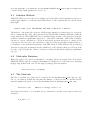
4.2
Molecular Database
Enter the path to the directory DataBase, containing all the molecular data, from where
MOLPOP-CEP is run. For example, if DataBase is a subdirectory of the directory containing
molpop.inp (which is the case for the zipped package) then the input is
Data directory = DataBase
4.3
The Molecule
The list of available molecules can be found in the file DataBase/mol list.dat (see §6).
Choose one name from that list and enter the number of energy levels to be included in the
run; this number should not exceed the maximum listed in DataBase/mol list.dat:
Molecule = CO
Number of energy levels = 11
Most listed molecules do not include vib-rot transitions, and the next entry in this case
should be
vib_max =
0
Currently, the database contains one species, SiO, with data for the lowest 19 rotational
levels in the first four vibration states. In this case MOLPOP-CEP corrects for the finite
number of rotational levels in the ground vibrational level, as described in Lockett & Elitzur
(1992). The input is then
vib_max = 4
jmax = 19
rot_const = 1.04 K
where the third input parameter is the rotational constant in temperature units.
4.4
Physical Conditions
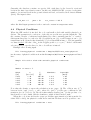
When the CEP method is invoked, the code can handle a slab with variable physical conditions. The parameters for each zone of the slab are read from a specified input file. The
file contains a header of arbitrary length limited by a line containing just the “>” symbol.
Subsequent lines list for each zone the (1) width in cm; (2) overall density in cm−3 ; (3)
temperature in K; (4) molecular abundance; (5) local linewidth in km s−1 . The last quantity
2
accountsqfor the local value of ∆νD in the Doppler profile e−[(ν−ν0 )/∆νD ] . If the local thermal
velocity 2kT /m exceeds c∆νD /ν0 , the code will use it instead.
Example: the following input
File listing physical conditions = Samples/CO/Flower_rates.physical
invokes entry of physical conditions from the file Samples/CO/Flower rates.physical listed
here:
Sample file with a slab with variable physical conditions
>
Number of zones = 5
Width
[cm]
2.d15
2.d15
2.d15
2.d15
2.d15
n
[cm^(-3)]
1.d4
1.d4
1.d4
1.d4
1.d4
T
[K]
100.d0
110.d0
120.d0
110.d0
100.d0
Abundance
1.d-4
1.d-4
1.d-4
1.d-4
1.d-4
Linewidth
[km/s]
1.d0
1.d0
1.d0
1.d0
1.d0
Note that the density n enters the calculation in two ways: (1) The collision rate (s−1 )
between levels i and j is Cij = nKij , where Kij (cm3 s−1 ) is the rate coefficient for the
transition (see §4.7 below). (2) The molecular number density (cm−3 ) is the product of n,
listed in the second column, and the abundance, which is listed in the fourth.
When the code is invoked in the escape probability approximation (solution method is
either LVG or slab), the physical conditions are uniform. In that case it is possible to use
File listing physical conditions = none
and enter the physical conditions directly in the input file as follows:
Gas Temperature = 100 K
n = 1.0e4 cm^-3
Molecular abundance (n_mol/n) = 1.0e-4
Velocity = 1 km/sec (linewidth for slab)
In the case of LVG calculations, the last entry becomes the expansion velocity instead of the
local linewidth and one must specify an additional entry, the logarithmic velocity gradient:
dlogV/dlogr = 1.0 (in effect only for LVG)
You can use this input method for physical conditions also in the case of CEP calculations
if the physical conditions in the slab are uniform.
Note: If the physical conditions are entered from a file, make sure your input
DOES NOT contain the last four (or five) entries. You can leave them in the
input file and just comment them out with the symbol %.
4.5
Line Overlap
Photons generated in a certain transition can be sometimes absorbed in another if the
linewidths exceed the frequency separation between the lines. This process is known as
line overlap or line fluorescence, and plays an important role in OH transitions and the
Bowen fluorescence phenomenon. Currently, MOLPOP-CEP can handle this effect only
when invoked in the escape probability mode (LVG or slab). The method of calculation is
described in Lockett & Elitzur (1989). To invoke this calculation use
overlap = on
For example, the input file Samples/OH/Offer rates.inp carries out a calculation taking
into account the effect of line overlap. Otherwise, enter overlap = off.
4.6
Maser Lines
When the optical depth of a line becomes negative, the intensity at this transition is amplified
by the medium in a maser effect. The following input determines whether the effect of the
maser radiation on the level populations (the “saturation effect”) is taken into account:
Include maser saturation (yes/no) = no
Selecting yes invokes an escape probability calculation for the saturation effect (see §5.3 in
Elitzur, 1992). This calculation can be selected only if the solution method is LVG or slab.
All CEP calculations must have no for the saturation entry. Calculations with the no option
produce the maser pump and loss rates that can be used to estimate maser emission from
the standard phenomenological maser model (see §5 below).
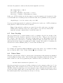
4.7
Collision Rates
As noted above (4.4), the collision rate between any two levels is nKij , where Kij (cm3 s−1 ) is
the rate coefficient for the transition and n is the overall density. MOLPOP-CEP can handle
an arbitrary number of collisional parters. The contribution of each one to the overall collision
rate is f nKij , where f is the fractional contribution of the particular collider, i.e., f n is the
collider density (in cm−3 ). These fractional abundances are entered as weight factors with
arbitrary scale, and MOLPOP-CEP takes care that the normalizations add up to 1. It is
also possible to scale each collisional rate independently by a factor so that it is possible to
experiment what happens when one of the collisional partners is neglected or its collisional
efficiency is increased by an arbitrary factor. There are a number of options for entering the
individual rate coefficients Kij themselves.
4.7.1
Tabulated Cross Sections
The most common entry of collision rates is from tabulations in files; this option is selected
with the keyword TABLE. The next entry specifies the name of the data file listing the
collisional rate between each pair of levels at a set of different temperatures; a file with
this name must exist in subdirectory Coll of the database directory specified in the second
input entry (see §6 below). MOLPOP-CEP interpolates between these temperatures if the
input value falls between two tabulated ones. If the prescribed temperature is outside the
tabulated range, MOLPOP-CEP will extrapolate according to the selection made with the
next keyword. When CONST is selected, MOLPOP-CEP will use the same value as the
largest or smallest tabulated √
temperature, as appropriate. Selecting SQRT(T) invokes an
extrapolation proportional to T from the appropriate border. Example:
Number of collision partners
weight
collision rates option
data file
extrapolation (SQRT(T) or CONST)
scaling factor
weight
collision rates option
data file
extrapolation (SQRT(T) or CONST)
scaling factor
=
=
=
=
=
=
=
=
=
=
=
2
1
table
CO_H2o.kij
sqrt(T)
1.0
1
table
CO_H2p.kij
sqrt(T)
1.0
This input will produce collisions with an equal mix of ortho- and para-H2 , with collision
rates from Flower (2001).
4.7.2
Hard-Sphere Collisions
This collision law, invoked with the keyword HARD SPHERE is available for all molecules. In
this analytic approximation, all downward collision rate per sub-level are equal to the the
same value σvT , where σ is a common input cross section and vT is the local thermal speed.
The sample input file OH/Hard Sphere.inp is an example:
Number of collision partners
weight
collision rates option
x-section
scaling factor
4.7.3
=
=
=
=
=
1
1
hard_sphere
1.e-15 cm^2
1.0
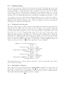
SiO Rotation-Vibrations
This collision law, invoked with the keyword SiO ROVIB is available only for SiO. It involves
SiO excitations in collisions with H2 , using the approximate theory of Bieniek & Green
(1983). This option is utilized in the sample input file SiO/SiO.inp:
Number of collision partners
weight
collision rates option
scaling factor
4.8
=
=
=
=
1
1
SiO_ROVIB
1.0
External Radiation
The cosmic microwave background (CMB) blackbody radiation at a temperature of TCMB =
2.725 K is always included. In addition, a number of other radiation fields can be added
and in each case the radiation can illuminate either side of the source or both. Furthermore,
the molecules can be immersed in a radiation bath with the specified spectral shape. This
is specified with the keywords left, right, both and internal. Note that distances into
the slab are measured from its left side.
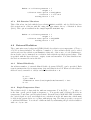
4.8.1
Diluted Blackbody
An arbitrary number of external diluted blackbody terms, W Bν (T ), can be specified. Each
term is parameterized by its temperature T bb and dilution factor W. When several radiation
fields are used, remember to always end the list with the W = 0:
W = 0.1
T_bb = 2500 K
Illumination from (left/right/both/internal) = left
W = 0.
4.8.2
Single-Temperature Dust
The radiation field of dust with the uniform temperature T is Bν (T )(1 − e−τν ), where τν
is the dust overall optical depth at frequency ν. You specify such a radiation field by its
temperature T and dust optical depth at visual. From the latter, MOLPOP-CEP determines
the optical depth at every wavelength from a tabulation in the file dust.dat, which must
be kept in the parent directory, together with molpop.inp. The dust properties correspond
to standard ISM dust. You can use a different dust by substituting the provided tabulation
with one of your own.
MOLPOP-CEP can handle an arbitrary number of such radiation fields. The list is
terminated by an entry with zero optical depth:
Dust tau at visual = 3.
Dust temperature = 100 K
Illumination from (left/right/both/internal) = internal
Dust tau at visual = 0.
4.8.3
Radiation Field from a File
Any spectral shape for the radiation field can be entered as a tabulation in a file, whose name
is specified as input. The Rtabulation should list the normalized spectral shape λFλ /Fbol (=
νFν /Fbol ), where Fbol = Fλ dλ is the bolometric flux, as a function of wavelength λ in
µm. The flux level at the molecular source is specified through the overall luminosity of the
radiation source and the distance to it:
Radiation from file = spectral.dat
Luminosity = 1.E4 Lo
Distance from source = 1.E15 cm
Illumination from (left/right/both) = left
To signal the end of spectral input files or that there is no input from a file altogether enter
Radiation from file = none
4.9
Solution Controls
Whichever solution method is invoked, MOLPOP-CEP solves the non-linear level population
equations with an iteration method—either Newton or accelerated Λ-iterations. The solution
accuracy and an upper bound on the number of allowed iterations are controlled as follows:
Accuracy in solution of the equations
Maximum number of iterations to solve
= 1.0e-3
= 50
You may try to solve the level populations for a desired input straightforward without any
attempt to improve the convergence. In that case, enter
Solution strategy = fixed
However, this may cause numerical difficulties. To aid convergence, MOLPOP-CEP offers
a step-by-step strategy. Starting from a situation in which the solution is known, the code
changes the column density in small increments using the solution from the previous step
as the initial guess for the next one. The exact solution is readily obtained in two limiting
cases. When all optical depths are zero (the optically thin limit) the statistical rate equations
for the level populations are linear and can be easily inverted. The solutions serve as the
starting point for an increasing strategy, in which the column density increases up to a
desired value. When all optical depths are very large, all the level populations thermalize,
following the Boltzmann distribution at the local temperature. Thermal populations serve
as the starting point for the decreasing strategy, in which the column density decreases
until the desired value is reached. In each case you have to specify an initial target that
serves as the smallest/largest value for all optical depths of the initial solution. The next
three entries control the sizes of the steps. The initial step size, entered as the number of
steps per decade, controls also the intervals for output printing. If at any point the step
size is too large, MOLPOP-CEP will keep decreasing it until it either achieves a successful
solution1 or bumps against either of the two limits set in the input: a lower limit on the step
size, entered through the maximum number of steps allowed per decade, and an upper limit
on the total number of steps allowed throughout the entire run. The variation of column
density is terminated when either physical dimension or the overall column density reaches
a prescribed upper/lower limit. Here’s an example of the increasing strategy:
Solution strategy = increasing
start with all optical depths less than tau_m
Initial number of steps per decade
Maximum number of dimension steps allowed per decade
Total number of steps allowed to reach any limit
stop when dimension exceeds R_m
or total column exceeds N_col
=
=
=
=
=
=
1
4
20
100
1.0E20 cm
1.E26 cm^-2
In a decreasing input, tau m would be a large optical depth providing a lower limit for all
transitions in the initial solution while R m and N col, the stopping criteria for the convergence process, would have values smaller than the desired target.
When solving the radiative transfer problem using the CEP method, it is possible to let
the code use a grid refinement technique to approach the exact solution of the problem. This
grid refinement systematically increases the number of zones in which each original zone is
subdivided until the maximum relative change in the level populations between one grid and
the next finer grid falls below a given threshold. The code also allows the user not to apply
the grid refinement technique and solve the radiative transfer problem in the given grid.
This strategy is chosen by using a zero:
Precision in CEP grid convergence (0 to ignore convergence) = 1.d-1
5
Output
MOLPOP-CEP offers a printout of parts, or all, of the molecular data. This allows you to
check that the data were entered properly. Printing is controlled with on and off switches:
Print energy level data
statistical weights g_i
energy in cm^{-1}
energy in GHz
1
=
=
=
=
off
on
on
on
If a successful solution is achieved with a smaller step size than originally prescribed, MOLPOP-CEP
will attempt to gradually increase the step size once it has passed the rough spot that caused problems. The
number of steps per decade will never be smaller than the initial one.
energy in K
= on
quantum numbers
= on
Print transition data
= on
wavelength in micron
= on
energy in GHz
= on
energy in K
= off
Einstein coefficients A_ij = on
collision rates C_ij
= on
Stop after printing molecular data = off
In this example, the energy level data will not be printed, even though individual switches
are on, because the master switch for these data is off. The last switch even allows you
to just produce a data tabulation without running MOLPOP-CEP at all. Also, when the
physical conditions vary in the slab, a printout of the collision rates, if requested, will cover
only the first zone.
Next you control the amount of output the program produces during the run. The
different printing options are controlled with on and off switches; in the following example,
all options are turned off by the master switch:
Progress print control
Messages from NEWTON
Messages from step-size selector
Messages from CEP progress
Printing output for initial guess
=
=
=
=
=
off
on
on
on
on
Note that whenever the CEP method is selected, MOLPOP-CEP will report its progress on
the screen irrespective of the output switches; that is, the above listed switch only controls
the printed output.
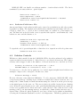
The default output, always produced by MOLPOP-CEP, contains a summary as follows:
R
cm
1.000E+16
1.778E+16
3.162E+16
Tot column
cm-2
1.000E+20
1.778E+20
3.162E+20
mol column
cm-2
1.000E+16
1.778E+16
3.162E+16
emission
erg/s/mol
8.557E-21
8.288E-21
7.928E-21
The last column is the overall cooling rate from all the transitions included in the calculation.
Additional output can be produced by turning on appropriate switches. For every printing
step, you can output: (1) Detailed level populations for all the transitions. (2) Information
on all inverted lines, if any exist. This output will include the optical depth, excitation temperature and inversion efficiency. (3) Information on the prescribed number of top thermal
emitting lines (note, there are no more then 12 N ×N transitions among N levels!):
Information on each step
print detailed populations
information on all inverted lines
Number of cooling lines to print (0 to bypass)
=
=
=
=
on
off
on
15
Finally, you can select some specific transitions for special output that will be listed at the
end of the run in summary form. Enter a number different from 0 (up to 10) for the number
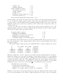
of transitions and then enter a pair of level identifier numbers for each transition. The
following example selects a summary output for the J = 1 → 0 and J = 7 → 6 rotational
transitions of CO:
the number of transitions = 2
i = 2
j = 1
i = 8
j = 7
For each transition, the output lists the excitation temperature, optical depth and the line
emission (erg/s/mol). If the transition is inverted, the last quantity is listed as zero. Instead,
the output lists quantities relevant for the standard, phenomenological maser model (see
Elitzur, 1992): The inversion efficiency, pump rate for each level, loss rate for each level and
their average.
The input file fname.inp produces the output file fname.outin the same directory. This
is the only output file produced in the single-zone escape probability case. When the CEP
option is used, additional files are generated as output, with the intermediate extension CEP
added to the name of the input file. For instance, for the Samples/CO/Flower rates.inp
input file, the following output files are generated:
• Samples/CO/Flower rates.out — main output file
• Samples/CO/Flower rates.CEP.trad — equivalent radiation temperature for each
transition and zone
• Samples/CO/Flower rates.CEP.pop — population of each level for each zone
• Samples/CO/Flower rates.CEP.slab — final slab partitioning in the converged solution
• Samples/CO/Flower rates.CEP.flux — line profiles of emergent flux in each selected
transition
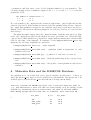
6
Molecular Data and the BASECOL Database
As explained above, molecular data can be placed anywhere provided the root directory
where the file mol list.dat is located is indicated in each input file. The master list of all
available species is in the file mol list.dat with the following current listing:
This file contains the MOLPOP molecular list. A molecule whose mol_name is,
e.g., XYZ should have a data file XYZ.lev with listing of N_lev energy levels
and XYZ.aij tabulating their A-coefficients. mol_mass is the mass number.
When adding another molecule make sure to terminate data lines with CR.
mol_name
N_lev
mol_mass
>
’CO’
’H2O_ortho’
’H2O_para’
41
48
48
28.0
18.0
18.0
’OH’
’SiO_vib’
32
100
17.0
44.0
This file is an index for the available molecules and the maximum number of levels included
in each model. Furthermore, the molecular mass (in atomic mass units) is also given. A
new species can be added as simply another entry line. It is important to terminate the last
entry with a CR. All the lines before the line containing only the symbol “>” are treated
as header. The same applies to the rest of files defining the energy levels, radiative and
collisional transitions.
6.1
Energy levels
The energy levels of species mol name are specified in the corresponding file mol name.lev.
For example, here are the first few lines from CO.lev:
Rotational energy levels for the ground state of CO
Reference: CDMS
N
g
1
2
3
4
5
1
3
5
7
9
Energy in cm^{-1}
Level details
>
0.0000
3.8450
11.5350
23.0695
38.4481
’J
’J
’J
’J
’J
=
=
=
=
=
0’
1’
2’
3’
4’
The listing must be ascending in energy. The statistical weight g is entered as integer, energy
is in cm−1 . Each level is internally identified in MOLPOP-CEP by the running number listed
in the first column. The level details are all read by MOLPOP-CEP as a single string and
used only for information in the output.
6.2
Radiative Transitions
The Einstein coefficients for spontaneous emission (Aij ) of species mol name are specified in
file mol name.aij; here are the first few lines from CO.aij:
Einstein coefficients A_ij for CO
Reference: CDMS
i
j
A_ij in s^{-1}
2
3
4
5
6
1
2
3
4
5
7.203e-08
6.910e-07
2.497e-06
6.126e-06
1.221e-05
>
6.3
Collisional Rates
As already mentioned (see §4.7), there are several options for specifying collision rates. The
most common is to supply tabulations in a file. A master list of all collision rate files is kept
in the file collision tables.dat inside the directory Coll/. The file lists the filename with
the collisional data together with two lines for comments that will be copied to the output
files, and terminated by a separator:
List of available tables of collision rates.
>
H2Oo_H2.kij
Collision rate coefficients for H2O_ortho-H2 collisions; corrected from H2O-He
Green et al 1993, ApJS 85, 181
******************
H2Op_H2.kij
Collision rate coefficients for H2O_para-H2 collisions; corrected from H2O-He
Green et al 1993, ApJS 85, 181
******************
OH_H2o.kij
Collision rate coefficients for OH-H2_ortho collisions
Offer et al 1994, JCP 100, 362
******************
OH_H2p.kij
Collision rate coefficients for OH-H2_para collisions
Offer et al 1994, JCP 100, 362
******************
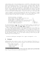
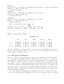
Here are the first few lines from OH H2o.kij:
Collision rate coefficients for OH-H2_ortho collisions.
Reference: Offer et al., 1994, J. Chem.Phys., 100, 362
>
Number of temperature columns = 5
I
2
3
3
4
J
1
1
2
1
TEMPERATURE (K)
15.0
50.0
100.0
150.0
200.0
0.40E-10
0.17E-09
0.58E-10
0.35E-10
0.39E-10
0.24E-09
0.71E-10
0.43E-10
0.34E-10
0.26E-09
0.72E-10
0.43E-10
0.31E-10
0.25E-09
0.69E-10
0.41E-10
0.28E-10
0.24E-09
0.65E-10
0.39E-10
The rate coefficients are entered in cm3 s−1 . Only downward (de-excitation) rates need be
specified. The program accounts for excitation rates via the Boltzmann detailed-balance
relation. Elastic collisions are ignored.
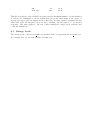
6.4
The Basecol Database
The Basecol bibliographic and numerical database was established at Meudon Observatory to address the community needs for data on molecular excitations. Accessible at
http://basecol.obspm.fr/, Basecol stores extensive information on molecular frequencies, transition rates and collisional excitations. The Basecol team has embarked on the
development of a web tool that remotely accesses their database and creates atomic and
molecular data files in the MOLPOP-CEP input format on the user’s local computer. The
Basecol web access tool will be part of the public MOLPOP-CEP package, which will enable
exact data analysis of line emission from multi-level systems with the most current atomic
and molecular data at all times.
A tool has already been included in the distribution at directory Basecol that generates all collisional information in MOLPOP-CEP format. Uncompress it and you will find
instructions on how to proceed to download data. The directory DataBase Basecol contains previously downloaded data that can be overwritten with new data. The input file
Basecol.inp, included in the samples, triggers a MOLPOP-CEP run that utilizes molecular
data files generated by the Basecol/MOLPOP tool.
A
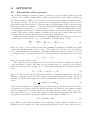
A.1
APPENDIX
Formulation of the problem
The standard multilevel radiative transfer problem in a given domain requires the joint
solution of the radiative transfer (RT) equation (which describes the radiation field) and
the kinetic equations (KE) for the atomic or molecular level populations (which describe
the excitation state). In the most general case, the numerical solution of this non-local
and non-linear problem requires to discretize the model atmosphere in N P zones where the
physical properties are assumed to be known. The standard multilevel RT problem consists
in obtaining the populations, nj , of each of the j = 1, 2, . . . , N L levels included in the atomic
or molecular model that are consistent with the radiation field created inside the complete
domain. This radiation field contains contributions from possible background sources and
from the radiative transitions in the given atomic/molecular model.
Making the usual assumption of statistical equilibrium, the rate equation for each level i
at each spatial point reduces to (e.g., Socas-Navarro & Trujillo Bueno, 1997):
X
j<i
Γji −
X
j>i
Γij +
X
j6=i
nj Cji − ni
X
Cij = 0,
(1)
j6=i
where Cij is the so-called collisional rate that quantifies the number of transitions per unit
volume and unit time between levels i and j. The symbol Γlu stands for the net radiative
rate, which quantifies the net number of radiative transitions between a bound lower level l
to an upper level u. Its expression in terms of the populations of the upper and lower levels
is:
Γlu = nl Rlu − nu Rul ,
(2)
where Rij are the radiative rates.
The collisional rates are assumed to be known and given by the local physical conditions
of the atmosphere. On the other hand, the net radiative rates Γlu depend on the radiation
field that is present in the domain. For bound-bound transitions, the following expression
holds:
Γlu = (nl Blu − nu Bul )J¯lu − nu Aul ,
(3)
where Aul , Bul and Blu are the spontaneous emission, stimulated emission and absorption
Einstein coefficients, respectively. The radiation field is parameterized in terms of the mean
intensity J¯lu , which is the frequency averaged mean intensity weighted by the line absorption
profile:
Z
1 Z
¯
Jlu =
dΩ dνφlu (ν, Ω)IνΩ ,
(4)
4π
where φlu (ν, Ω) and IνΩ are, respectively, the normalized line profile and the specific intensity
at frequency ν and direction Ω. The specific intensity is governed by the radiative transfer
equation, which can be formally solved if we know the variation of the opacity (χν ) and of
the source function (ǫν /χν , being ǫν the emission coefficient) in the medium. Once the stellar
atmosphere is discretized, the specific intensity can be written formally as
IνΩ = ΛνΩ [Sν ] + TνΩ ,
(5)
where TνΩ is a vector that accounts for the contribution of the boundary conditions to the
intensity at each spatial point of the discretized medium, Sν is the source function vector
and ΛνΩ is an operator whose element ΛνΩ (i, j) gives the response of the radiation field at
point “i” due to a unit-pulse perturbation in the source function at point “j”.
Since the radiative transfer equation couples different parts of the atmosphere and the
absorption and emission properties at all the spatial points depend on the level populations,
the RT problem is both non-local and non-linear. Therefore, the system of Eqs. (1) represents a highly non-linear problem. This non-linearity makes it necessary to apply suitable
iterative methods. Among them, the simplest one is the Λ-iteration (e.g., Mihalas, 1978),
in which, starting from an initial estimation of the populations, the mean intensity at each
transition is obtained through Eq. (4) and plugged into Eqs. (1). The resulting linear system
is solved and the iteration is repeated. This scheme works correctly when the optical depth
of all transitions is less than unity but the convergence time increases dramatically if any
transition is optically thick. The reason is that the iterative scheme transfers information in
the domain in steps of the order of τ ≈ 1. In optically thick cases, it takes many iterations to
transfer information from one part of the domain to the others. The accelerated Λ-iteration
(Rybicki & Hummer, 1991, 1992) overcomes many of the convergence problems of the simple
Λ-iteration by rewriting the net radiative rates of Eq. (3) using a suitable combination of
population from the previous and the new iterative step, thus leading to an important improvement in the convergence properties. A modification of this method by Trujillo Bueno
& Fabiani Bendicho (1995) leads to the Gauss-Seidel and Successive Overrelaxation methods that produce an improvement in the convergence rate of up to an order of magnitude.
Finally, methods based on multigrid iterations Steiner (1991); Fabiani Bendicho et al. (1997)
have also been applied to the radiative transfer problem with success.
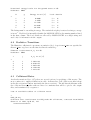
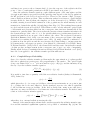
A.1.1
Coupled Escape Probability
Our code solves the radiative transfer problem under the approximation of a plane-parallel
slab whose physical properties vary only perpendicular to the surface. The optical depth
along a ray slanted at θ = cos−1 µ from normal is τν (µ) = τ Φ(x)/µ, and the intensity along
the ray obeys the radiative transfer equation:
µ
dIν (τ, µ)
= Φ(x)[S(τ ) − Iν (τ, µ)].
dτ
(6)
It is useful to introduce a quantity called the net radiative bracket (Athay & Skumanich,
1971), defined by:
¯ )
J(τ
,
(7)
p(τ ) = 1 −
S(τ )
which plays the role of a escape probability so that the mean intensity at one point is just
(1 − p) times the local source function. In the standard one-zone case, this is equivalent
to the well-known escape probability. If the slab is divided into many zones, this factor
takes into account correctly the no-local character of the radiative transfer. From the formal
solution of the radiative transfer equation,
p(τ ) = 1 −
Z ∞
Z 1
1 Z τt
dµ
S(t)dt
Φ2 dx e−|τ −t|Φ/µ
2S(τ ) 0
µ
−∞
0
(8)
when there is no external radiation entering the slab.
Instead of the usual iterative scheme that consider separately the radiative transfer equation and the statistical equilibrium equations, it is possible to substitute Eq. (8) into the
net radiative rate, resulting in:
Γlu = −nu Aul p(τ ),
(9)
which demonstrates that the only radiative quantity actually needed for the calculation of
level populations at every position is the net radiative bracket p(τ ). Once this factor is known
at each zone of the domain, we could compute the level populations that are consistent with
the radiation they produce without solving for the intensity. It is evident from Eq. 8 that the
factor p(τ ) itself can be computed from the level populations, again without solving for the
intensity. Therefore, inserting p(τ ) from equation 8 into the radiative rate terms produces
level population equations that properly account for all the effects of radiative transfer without
actually calculating the intensity itself.
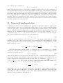
B
Numerical implementation
A numerical solution of the resulting level population equations requires a spatial grid,
partitioning the source into zones such that all properties can be considered uniform within
each zone. The degree of actual deviations from uniformity, and the accuracy of the solution,
can be controlled by decreasing each zone size through finer divisions with an increasing
number of zones. Assume that the slab is partitioned into z zones. The i-th zone, i = 1 . . . z,
occupies the range τi−1 < τ ≤ τi , with τ0 = 0 and τz = τt , with τt the total optical depth.
The optical depth between any pair of zone boundaries is
τ i,j = |τi − τj |
(10)
so that the optical thickness of the i-th zone is τ i,i−1 . One has to remind that the optical
thickness of the i-th zone in a given bound-bound transition under the assumption of complete redistribution is given by the following linear combination of the populations of the
upper and lower levels:
hν
ν − ν0
τi (ν) =
(nl Blu − nu Bul ) Φ
i
4π
∆νD
!
(11)
Since the temperature and the density of colliders (H2 , H or e− ) is assumed to be constant
within each zone, the collisional rates Cij are constant in the zone. Correspondingly, the net
radiative rate is just given by
Γilu = −niu Aul pi ,
(12)
where the population of the upper level in each zone is also constant and the superscript i is
used as a zone label. Since the factor p(τ ) varies in the zone, it has to be replaced by a constant pi that
should adequately
represent its value there, for example pi = 21 [p(τi ) + p(τi−1 )]
or pi = p 12 [τi + τi−1 ]) . There are no set rules for this replacement other than it must obey
pi → p(τi ) when τ i,i−1 → 0. We choose for pi the zone average
i
p =
1
τ i,i−1
Z
τi
τi−1
p(τ )dτ,
(13)
which turns out to be one of the key ingredients of the success of the coupled escape probability. The reason is that the value of pi used in each zone is obtained as an average value
inside the zone of the true variation of p(τ ). The other possibilities assume a simple behavior
(linear) of the p(τ ) function inside the zone.
B.1
Internal radiation
From Eq. (8), calculation of pi requires an integration over the entire slab, which can be
broken into a sum of integrals over the zones. In each term of the sum, the zone source
function can be pulled out of the τ -integration so that
Z
τi
z
X
1
pi = 1 −
2τ i,i−1 S i
dτ
τi−1
Z
τj
dt
τj−1
j=1
Z
Sj ×
∞
Φ2 dx
−∞
Z
1
0
e−|τ −t|Φ/µ
dµ
µ
(14)
The remaining integrals can be expressed in terms of common functions. Consider for example
1
βi = 1 −
Z
τi
2τ i,i−1
dτ
τi−1
Z
τi
×
dt
τi−1
Z
∞
Φ2 dx
−∞
Z
0
1
e−|τ −t|Φ/µ
dµ
,
µ
(15)
the contribution of zone i itself to pi . It is straightforward to show that β i = β(τ i,i−1 ), where
Z 1
1Zτ Z∞
dt
Φ(x)dx dµ e−tΦ(x)/µ
β(τ ) =
τ 0
−∞
0
(16)
This function was first introduced by Capriotti (1965). It represents the probability for
photon escape from a slab of thickness τ , averaged over the photon direction, frequency and
position in the slab. The contribution of zone j 6= i to the remaining sum can be handled
similarly, and the final expression for the coefficient pi turns out to be very simple:
pi = β i +
z
1 X
S j ij
M
τ i,i−1 j=1 S i
(17)
j6=i
where
1
(18)
M ij = − (αi,j − αi−1,j − αi,j−1 + αi−1,j−1 )
2
and where αi,j = τ i,j β(τ i,j ). The quantity αi,j obeys αi,j = αj,i and αi,i = 0, therefore M ij =
M ji and M ii = αi,i−1 . The first term in the expression for pi is the average probability for
photon escape from zone i, reproducing one of the common variants of the escape probability
method in which the whole slab is treated as a single zone (e.g., Krolik & McKee, 1978). The
subsequent sum describes the effect on the level populations in zone i of radiation produced in
all other zones. Each term in the sum has a simple interpretation in terms of the probability
that photons generated elsewhere in the slab traverse every other zone and get absorbed in
zone i, where their effect on the level populations is similar to that of radiation external to
the slab.
Inserting the final expression for pi from Eq. (17) into the rate terms of Eq. (9) in every
zone produces a set of non-linear algebraic equations for the unknown level populations
nik . The solution of these equations yields the full solution of the line transfer problem by
considering only level populations. The computed populations are self-consistent with their
internally generated radiation even though the radiative transfer equation is not handled at
all.
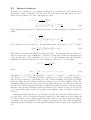
B.2
Numerical evaluation of the auxiliary functions
Although the couple escape probability overcomes the solution of the radiative transfer
equation, it is necessary to evaluate the τ -dependent auxiliary function β(τ ). In order to
speed up the evaluation of these functions, we tabulated it for 1000 points in τ and a spline
interpolation routine is used to calculate its values at any other value of τ not in the database.
We have verified that this approach gives computational times comparable to those given by
using the approximate formula of Krolik & McKee (1978) but the reached precision is much
larger.
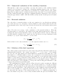
B.3
External radiation
The only effect of external radiation on the rate equations is to modify the net radiative
i
rate of the i-th zone as a consequence of the modification of the radiation field. If J¯int
is the
mean intensity in the i-th zone produced by the slab itself, the total radiation field is given
by:
i
i
J¯i = J¯int
+ J¯ext
(19)
i
where J¯ext
is the zone average of the contribution of the external radiation. When the
i
external radiation corresponds to the emission from dust which permeates the source, J¯ext
is simply the angle-averaged intensity of the local dust emission in the i-th zone. When the
external radiation originates from outside the slab and has an isotropic distribution with
intensity Ie (= Je ) in contact with the τ = 0 face, then
1 i
J¯ext
= 12 Je i,i−1 αi,0 − αi−1,0 .
τ
(20)
If the radiation is in contact with the τ = τt , the expression turns out to be:
1 i
J¯ext
= 21 Je i,i−1 αi,z − αi−1,z .
τ
B.4
(21)
Solution of the final equations
The solution method just described is exact in the sense that the discretized equations are
mathematically identical to the original ones when τ i,i−1 → 0 for every i. As is usually
the case, the only approximation in actual numerical calculations is the finite size of the
discretization, i.e., the finite number of zones. As a consequence, if one is interested in solving
the problem up to a given precision in the level populations, one should start with an initial
number of zones and stop when the relative change between one grid and a refined one in
which a suitable regridding strategy is applied is below a predefined tolerance. MOLPOPCEP allows the user to select whether to converge the solution using grid refinement or just
converge the problem in a predefined grid.
The actual numerical solution of the set of Eqs. (1) can be carried out using two different
techniques. The most straightforward is to use a Newton method to solve the non-linear
equations. The interesting key point is that the Jacobian matrix can be calculated analytically because the dependence of the radiation field on the population is known analytically.
The second possibility is to apply the Λ-iteration method. The diagonal of the Λ operator, that gives the response of the radiation field at zone j to a unitary perturbation of
the source function at point i, can be easily calculated under the previous formalism. This
second method of solution can be competitive when the numerical inversion of the Jacobian
turns out to be too time consuming.
In order to improve the convergence properties of the code, the following strategy is
applied the solution of the statistical equilibrium equations. This is of special interest for
the case in which the physical conditions are constant. Two possible possibilities exist: start
from a molecular column density in which all the lines are optically thin (τ < 1) or start
from a molecular column density in which all the lines are optically thick (τ ≫ 1). In the
first case, the level populations should be close to the optically thin solution and this can be
chosen as the initial condition. In the second case, the level populations should be close to
local thermodynamical equilibrium (LTE) and the Boltzmann distribution can be assumed
as an initial condition. Then, the molecular column density is either reduced or increased in
steps until some suitable limits in the column density are reached. This strategy allows the
code to increase the convergence behavior and, as a subproduct, the solution is obtained for
many intermediate problems.
If the final solution is far from any of the limiting cases (optically thin or LTE populations), the Newton method can suffer from convergence problems. Another remedy for
this difficulty that we plan to investigate in the future is to carry out several accelerated
Λ-iterations starting from one of the limiting cases (hopefully the closer to the final solution)
and then apply the Newton method for the solution refinement. Although the accelerated
Λ-iteration can also suffer from convergence problems if started far from the solution, they
are less important than for the Newton scheme.
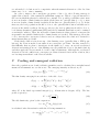
C
Cooling and emergent radiation
Once the populations are found, radiative quantities can be calculated in a straightforward
manner from summations over the zones. The emerging intensity at direction µ is
Iν (τt , µ) =
z X
e−τ
i=1
z,i Φ/µ
− e−τ
z,i−1 Φ/µ
S i.
(22)
The flux density emerging from each face of the slab obeys
Fν (τt ) = 2π
z h
X
i=1
−Fν (0) = 2π
z h
X
i=1
i
E3 (τ z,i Φi ) − E3 (τ z,i−1 Φi ) S i
i
E3 (τ i−1,0 Φi ) − E3 (τ i,0 Φi ) S i
(23)
where E3 is the third exponential integral (e.g., Abramowitz & Stegun, 1972). The line
profile is given by:
!
ν − ν0
i
Φ =Φ
(24)
i
∆νD
The slab luminosity, given by the expression:
Λ = 4π
Z
0
τt
∆νD S(τ )p(τ )dτ,
(25)
is calculated after discretization with the following summation:
Λ = 4π
z X
i=1
αi,0 − αi−1,0 − αz,i + αz,i−1 S i .
(26)
References
Abramowitz, M., & Stegun, I. A. 1972, Handbook of Mathematical Functions (New York:
Dover)
Athay, R. G., & Skumanich, A. 1971, ApJ, 170, 605
Bieniek, R. J., & Green, S. 1983, ApJL, 265, L29
Capriotti, E. R. 1965, ApJ, 142, 1101
Elitzur, M. 1992, Astronomical Masers (Dordrecht: Kluwer Academic Publishers)
Elitzur, M., & Asensio Ramos, A. 2006, MNRAS, 365, 779
Fabiani Bendicho, P., Trujillo Bueno, J., & Auer, L. H. 1997, A&A, 324, 161
Flower, D. R. 2001, J. Phys. B, 34, 2731
Krolik, J. H., & McKee, C. F. 1978, ApJS, 37, 459
Lockett, P., & Elitzur, M. 1989, ApJ, 344, 525
—. 1992, ApJ, 399, 704
Mihalas, D. 1978, in Stellar Atmospheres, Vol. 455
Rybicki, G. B., & Hummer, D. G. 1991, A&A, 249, 720
—. 1992, A&A, 262, 209
Socas-Navarro, H., & Trujillo Bueno, J. 1997, ApJ, 490, 383
Steiner, O. 1991, A&A, 242, 290
Trujillo Bueno, J., & Fabiani Bendicho, P. 1995, ApJ, 455, 646