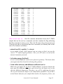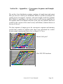
Download Arvert 4.0.1 - Earth and Environmental Sciences

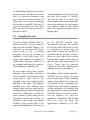
Arvert 4.0.1
Inversion of 40Ar/39Ar Age Spectra
User's Manual
Peter Zeitler
Earth & Environmental Sciences
Lehigh University
[email protected]
www.ees.lehigh.edu/geochronology.html
updated 23 June, 2004
1
User Agreement
Arvert is freeware. You can download, use, and modify it without cost.
However, your use of Arvert is subject to the following conditions:
•Please acknowledge use of this code
•You can’t sell or charge for the use of Arvert code, modified or not
•Notify me of any non-trivial changes you make
• I’ll try to help you if I can, but I’m under no obligation to provide
technical support in the downloading, compilation, operation, or use of
this program
•Lehigh University and Peter Zeitler take no responsibility for any errors
that might arise during the use of Arvert, due either to the code itself or in
the instructions for its use, and are not liable for any consequences of
such errors. I do promise to express chagrin if you find a howler.
•Please notify me of any bugs you find, and pass along suggestions for
improvements.
2
Contents
1. Introduction .........................................................................
1.1 What is Arvert? ........................................................
1.2 How does Arvert work?............................................
1.3 How is Arvert best used?..........................................
4
4
4
7
2. Obtaining and Installing Arvert..........................................
2.1 Getting code or applications .....................................
2.2 Overview of running the application.........................
2.3 Compiling the code ..................................................
9
9
9
10
3. Using Arvert.........................................................................
3.1 Program inputs and outputs ......................................
inputs (file crs.in) .................................................
inputs (file domains.in).........................................
inputs (file goal.in) ...............................................
inputs (file helium.in)............................................
outputs..................................................................
3.2 Viewing results.........................................................
3.3 Modeling considerations...........................................
while modeling .....................................................
when you’re done .................................................
3.4 Warnings and issues .................................................
11
11
11
19
21
22
24
26
26
26
27
28
4. Special Topics ......................................................................
4.1 History of Arvert ......................................................
4.2 Performance .............................................................
4.3 Future versions of Arvert..........................................
32
32
33
34
5. References and Suggested Reading .................................... 35
6. Appendix – Convergence Sequence, Sample Results ....... 36
3
Section One – Introduction
1.1
What is Arvert?
Arvert is a numerical model that
inverts K-feldspar 40Ar/39Ar age
spectra for thermal history. Given a
measured age spectrum and kinetic
and domain parameters determined
from the 39Ar released during the
step-heating experiment, Arvert will
try to find those thermal histories
that would result in an age spectrum
like the one measured. The latest
version of Arvert can include He age
data in the inversion.
This manual assumes that readers
and prospective users of Arvert have
an understanding of geochronology
and know the basic principles of
thermochronology, including the
multi-domain model for argon
diffusion in feldspars.
So, if the first paragraph was Greek
to you, Run Away!
1.2 How does Arvert work?
Being an inverse model, Arvert
attempts to determine fundamental
controlling parameters (i.e., a
thermal history) from observations
of a complex observed phenomenon
(i.e., an age spectrum, and a UTh/He age). The program has two
main components, a pair of forward
models that can calculate an age
spectrum and helium age for a given
thermal history, and an algorithm
that reshapes a starting pool of
random thermal histories into a set
of solutions that increasingly
minimize the mismatch between
calculated and observed age spectra
and He ages.
The core forward model is taken
from Oscar Lovera’s original code
for the calculation of age spectra
from samples incorporating multiple
diffusion domains (Lovera et al.,
1989). Thus, at its heart, Arvert is
completely dependent on the
assumptions that go into the
multidomain diffusion (MDD)
model. There is now an extensive
literature on this subject and some
excellent work and reviews by the
UCLA group on the validity of this
Arvert 4.0.1 User’s Manual
Page 4
conceptual model as a description
for Ar diffusion in feldspar. If for
some reason you reject the MDD
model, then Arvert is not the
program for you. The text by
McDougall and Harrison (1999) is
an excellent place to start for a
discussion of 40Ar/39Ar thermochronology and the MDD model.
To be clear, here are the
assumptions upon which Arvert is
based:
Ar diffusion in feldspars occurs by
volume diffusion, with similar
mechanisms and kinetics operating
in nature as during 39Ar extraction in
the laboratory.
Feldspars are divided into discrete
diffusion domains of differing sizes
(or diffusivity, or both). Although
the code can handle domains of
differing activation energy,
experience shows this to be
unnecessary (the code expresses
variation among domains in terms of
size variation but mathematically,
variations in D have exactly the
same influence as variations in size).
Arvert assumes that variations
within an age spectrum are entirely
due to accumulation of 40Ar by
radioactive decay and loss of 40Ar
by thermally activated diffusion
acting in the sample’s domain
structure: it is assumed that the
sample contains no extraneous Ar
components or that these have been
corrected for.
The inverse portion of the Arvert
code uses the controlled random
search (CRS) algorithm of Price
(1977) as adapted by Willet (1997)
for the inversion of apatite fissiontrack data. This algorithm retains the
advantages of a Monte Carlo
approach in searching parameter
space for true minima, while
converging far more rapidly due to
the “learning” component inherent
in the CRS method. It is beyond the
scope of this guide to discuss
inverse methods as they have been
applied to thermochronometric data;
see the article by Willett (1997) and
references therein as a start.
Arvert minimizes the misfit between
a measured age spectrum and those
that it calculates. This “objective
function” in the case of Arvert can
take two forms, either a simple
mean-percent deviation between the
steps of the observed and modeled
spectra and He age, or a mean
square of weighted deviates that
takes into account assigned errors on
each heating step and the He age.
In detail, Arvert works as follows.
Initially, a pool of 100 to 300
thermal histories is randomly
generated, subject to any constraints
supplied by the operator (“explicit”
constraints are in the form of
maximum
and
minimum
Arvert 4.0.1 User’s Manual
Page 5
temperatures for the problem space;
“implicit” constraints are in the form
of maximum and minimum heating
and cooling rates). An age spectrum
is calculated for each thermal
history and its fit parameter is
determined. Next, the program goes
into its main loop, and begins to
sequentially create new thermal
histories, keeping or discarding
them depending on whether they
represent a better fit than the current
worst member of the pool; if a good
fit is found, the worst member of the
pool is discarded. The program
continues until it reaches the
specified number of iterations, or
has brought all histories in the pool
to converge within the specified
limits.
New CRS thermal histories are
made as follows. A subset of about
10 thermal histories is randomly
selected from the main pool, plus
one more. The histories in the subset
are averaged, and then a new history
is made by reflecting the additional
selected history through the
averaged values, subject to an
amplification factor that might range
between 1.1 and 1.5. Figure 1 gives
what is probably a more clear
depiction of this process.
Arvert 4.0.1 User’s Manual
Page 6
Figure 1.
CRS algorithm for
creating a new thermal
history.
1.3 How is Arvert best used?
Unless you start tinkering with its
code, or until you use it for a while,
Arvert will appear to you as the
quintessential black box, and it will
be tempting to treat it as such. Avoid
this temptation! Make an effort to
understand what the main inversion
parameters do, and how constraints
and parameters can bias your results,
sometimes in subtle ways.
Arvert is best used to investigate
what classes of thermal history
might serve as explanations for a
particular age spectrum, given
whatever firm geological constraints
you have in hand. Once you know
Arvert 4.0.1 User’s Manual
Page 7
what the possibilities are, one option
is to then continue using manually
directed forward modeling to
complete the fitting of the age
spectrum. However, this approach
sacrifices one of the potential
advantages of the inverse approach,
and that is to obtain a feeling for
confidence limits on various parts of
the derived thermal history. With
careful use and an understanding of
some of its pitfalls, Arvert can
provide this information (but see
Section 3.5).
What you should NOT do is just run
Arvert once for countless iterations,
and then take this single result as the
truth. You must make some effort to
see how different constraints
influence the model, and how well
your derived diffusion-domain
structure is permitting the model to
function (ill-defined kinetic and
domain data can make it difficult for
Arvert to fit parts of an age
spectrum, causing over-convergence
to false precision to occur for parts
of the thermal history). It is
important to remember that in many
applications of K-feldspar
thermochronology, your goal is an
understanding of process and
timing, at the level of precision that
geologic data and realistic, often
under-determined thermal models
can provide.
Given the current and improving
speed of most personal computers
and workstations, if you devote 2-3
hours to multiple background runs
of Arvert you should be in good
shape. Start by running multiple
models for only a few thousand
iterations each, perhaps changing
the duration of the model to permit
different prehistories to come into
play. Try allowing some (re)heating,
unless you are absolutely certain
that this could not apply. Alter the
number of time nodes to see whether
this is introducing an artifact for
your particular case. Check to see if
there is a portion of your age
spectrum that is not fitting well,
possibly due to an error in domain
structure. After all this, you can then
try a few final runs that continue for
longer durations and attempt to
achieve statistical convergence.
Arvert 4.0.1 User’s Manual
Page 8
Section Two – Obtaining and Installing Arvert
2.1 Obtaining code or applications
Arvert source code, a compiled
application, example inputs and
outputs, and helper applications
should be available at
http://www.ees.lehigh.edu/geochron
ology.html
Alternatively, as a second resort,
you can contact Peter Zeitler at
[email protected]
and I can email you the code and
any applications as attachments.
I use and develop Arvert under Mac
OS, so helper applications and the
compiled code will work only on
Macs. Most of these are Carbon
applications and will run under both
OS 9.x and OS X. If you wish to use
Avert on a different platform, you
will need to recompile and link the
source code (See Section 2.3).
2.2 Overview of running the application
For reasons of time (mine) and
programming incompetence (mine),
Arvert currently runs as a commandline program in a text window. At
some point I may figure out how to
bring the code into the modern
world, but I wouldn’t hold your
breath. The fact is that until
computer speeds increase by another
factor of 20 or so, Arvert will not be
an interactive program, so lack of a
GUI isn’t that big a deal.
To actually run Arvert, you just
double-click it’s icon. You are
presented with a list of what Arvert
thinks are your inputs. You should
check these for blunders or silly
values to avoid wasting time.
(Arvert does use assertions to check
for bad values, but there are still
many ways to launch useless runs).
Once you’ve checked your inputs,
your only options at this point are to
abort the run or to proceed.
Once the program is running, you
can pause it by typing cmd-P. This
will allow you to scroll back up the
text window and see what’s been
happening, which can be useful once
you’ve accumulated lots of lines of
progress reports. At any time, you
can quit the application in the
standard way, but you will
effectively lose your calculated data.
At the end of the run, just quit.
Arvert is an ok citizen with respect
Arvert 4.0.1 User’s Manual
Page 9
to multitasking, and you can switch
away from it to do other work. Note
that it is processor intensive and
may slow down the operation of
other tasks, so your Snood playing
will not be as enjoyable. Likewise, if
you pin the processor with other
jobs, you will slow down Arvert’s
progress as well.
You communicate with Arvert using
text files (See Section 3.1, below).
An obvious hint is to move the
Arvert application and its input files
into a new directory for each sample
you want to model so that Arvert
places its output directories into a
logical place.!
2.3 Compiling the code
If you are using a Wintel, Unix, or
Linux system, or you are using a
Mac but wish to make changes, you
will have to recompile the Arvert
source code to get a working
program. Arvert is written in
standard C (not ANSI strict). The
source code consists of a number of
small source files that will have to
be compiled and linked as a project.
This should be straightforward.
Several minor areas may require
attention. First, the Mac version of
Arvert includes a borrowed routine
(keystroke.c) that allows the
program to be more easily paused,
and this is Mac-only. The program
should work fine without this
option. Next, there are some calls to
standard timing routines that should
work but could cause a glitch on
some systems. Again, these can be
expunged without any trouble, or
rewritten if you really want timing
feedback. Next, on the Mac, I use
some included libraries to divert text
to the SIOUX window that
Metrowerks provides for console
I/O. In the header file arvert.h, there
is a reference to sioux.h that you
may need to delete on non-Mac or
non-Metrowerks systems. Finally,
there are a few calls to Mac system
routines that set file creator codes so
that the data files open directly in
Excel. These can be removed
without any ill effect, although this
amounts to a nice convenience.
Depending on the system, compiler,
and IDE you are using, you may
have to take steps to have standard
output using printf go to some sort
of window or the command line.
Finally, based on my dim memories
of past experience, it is possible that
you may run into some sort of glitch
with file import on some systems,
but the routines I’ve used are
standard C and simple, and all data
files are read in from the
application’s directory, so if any
Arvert 4.0.1 User’s Manual
Page 10
effort is required it should be
minimal.
For the record, I have been using
various versions of the everevolving Metrowerks IDE for Mac.
The included libraries under the IDE
are MSL_All_Carbon.Lib and
Carbon.Lib obtained via the Std C
Console stationary. I’ve turned on
all possible optimizations.
Good luck!
Section Three – Using Arvert
3.1 Program inputs and outputs
Inputs. To work, Arvert requires
four text files to be present in the
same directory as the application;
they must retain their exact names.
Within these files it is best to delimit
same-line parameters with tabs.
What follows is a lengthy discussion
of the contents of these files and,
where needed, a discussion of what
the parameters do and what ranges
of values to use. A fundamental
description of each parameter is
given in bold face; additional
comments on the parameter are in
italics. The files are c r s . i n ,
domains.in, goal.in, and
helium.in.
(File 1) crs.in – this file contains all the controlling parameters for the
inversion, and is the file you will be modifying between runs. The format is as
follows:
• String giving run info (maximum 100 characters)
• File suffix appended to output files (maximum 10 characters)
Not critical but very helpful in sorting output from different runs.
• Number of iterations for the CRS algorithm
Most runs will terminate based on this parameter. Usually it is not
worth doing fewer than 2000 iterations, but on the other hand resist the
urge to do too many iterations until you are ready, as you can always
Arvert 4.0.1 User’s Manual
Page 11
keep restarting the model after having a quick check of results. Usually
a total of 5000 to 20000 iterations will be sufficient.
• Model duration in millions of years
You should be sure to leave adequate model time before initial closure,
especially if you wish to permit reheating. Otherwise, your model
results may be unduly influenced by your chosen starting constraints.
On the other hand, it would be silly to run a 1000 Ma model for a
sample that was only 10 Ma in maximum age, as this would waste
compute time and lower the model resolution because most time nodes
would be wasted outside the region where the sample has constraining
power. Warning: you need to make sure that the model duration and
the time of the first explicit constraint (if any) are the same.
Unless you have data such as a U-Pb age to constrain your sample’s
higher-temperature history, you might want to leave 30-50 m.y.
between the start of the model run and the time of first closure. Tip:
Because Avert always uses 0 Ma as one of its model boundaries, if you
are modeling an older sample and know that more recent thermal
events are unlikely, you might consider engineering a static shift in
your data, lowering all the ages in your goal age spectrum by the same
amount. This will maximize the number of time nodes Arvert distributes
around the period of interest to your age spectrum.
• Number of time nodes (minimum of 2, maximum of 15)
The number of time slices at which Arvert generates temperatures. This
is a critical but subtle parameter. If the number is too high, at times
Arvert may crash because it will not be possible to generate legal
Monte-Carlo histories that satisfy all constraints (usually a problem
with models that allow heating). But if the number is too low, be aware
that you begin to limit the representation of the thermal history to only
a few line segments that are fixed and widely spaced in time; such a
model will not be able to handle histories with sharp inflections. The
absolute limit in nodes is 2, which gives you only the model start and its
end at 0 Ma, and means you will be modeling the thermal history as a
single line segment!
Generally speaking, you will want to keep your number of time nodes
about the same as the subset size (see Willett (1997)).
Arvert 4.0.1 User’s Manual
Page 12
You may wonder how Arvert distributes its time nodes. Early versions
of the program distributed them evenly. To allow better resolution at
times when temperatures might be changing, later versions permitted
the user to specify the time nodes. However, I felt that this permitted too
much fiddling and user intervention that might bias results. So, Arvert
4.x now distributes time nodes based on the lowest and highest ages in
the age spectrum. Two nodes always have to go to the start and end of
the model. If only three nodes are specified, Arvert tosses the one extra
node into the middle of the time span bracketed by the age spectrum. If
four are specified, Arvert places time nodes near the age maximum and
minimum. If more than four are specified, Arvert then tries to distribute
any remaining nodes across the age spectrum’s time span, putting a
little more effort into the regions near the maximum and minimum ages.
One advantage of this is that it minimizes wasted nodes in regions far
outside areas of interest. However, be aware that Arvert’s time nodes
may not jive perfectly with your sample’s needs, particularly if the
precise timing of a heating or cooling pulse is critical. If you suspect
this is the case, you can always try adding or subtracting a time node to
see if this makes a large difference in Arvert’s behavior.
Be aware that as the number of time nodes climbs, it will be
increasingly difficult for Arvert to make CRS histories that completely
satisfy the implicit constraints. If you think about the ball of yarn that is
the Monte Carlo pool, many combinations of these will produce a
segment or two that is too steep, or if only cooling is allowed, that
actually increases in temperature. By the time you reach 15 to 20 time
nodes, there is almost no chance that Arvert will satisfy your CRS
implicit constraints. At the moment, the program tries fully 1000 times
to make a legal history, and then gives up and takes the last one
generated. So, when the number of time nodes increases, the program
will slow a little as it churns through possible histories, and in many
cases your implicit CRS constraints will end up ignored. If you are
really bothered by this you can always filter your data manually after
the run.
One last note about time nodes and thermal histories. To try and
minimize progressive bias when generating the Monte Carlo histories,
Arvert uses an alternating approach developed by Sean Willett. Rather
than start from one end and making temperatures at sequential time
Arvert 4.0.1 User’s Manual
Page 13
nodes, Arvert first chooses a time node at random and then works up
and down as it makes each history.
• Number of constraining brackets for thermal histories
You can place explicit constraints on portions of the problem space in a
somewhat crude fashion by specifying permissible temperature ranges
at specific times (between these specified times Arvert just extrapolates
linearly). You must place at least two constraints on the model, and no
more than 10. The first and last constraints must be at the model start
and end (at times <modelduration> and 0 m.y.). If you don’t want to
enter any constraints, then simply choose to create two and make their
minimum and maximum temperatures be something like 0 ˚C and 500
˚C.
• N constraints, format: <time> <min Temp ˚C> <max Temp ˚C>
Enter as many rows of constraints as you have chosen, using the format
given above. Be sure that the time values decrease progressively. Also
be sure that the constraints don’t conflict with the implicit (rate)
constraints you specified, lest Arvert spit the dummy or get confused.
• Maximum heating and cooling rates for Monte-Carlo histories
You must specify what the maximum values for heating and cooling rate
are during the generation of the initial Monte-Carlo pool of thermal
histories. To rule out either cooling or heating, enter a value of 0 (the
units of this parameter are ˚C/m.y.). The permitted range is between 0
and 1000 ˚C/m.y.
Note that for typical models runs of 10 m.y. or more with upper
constraints of 500˚C or so, you will never be able to use a rate of 1000
˚C/m.y., since this would be equivalent to only 0.5 m.y. in time, and for
older models Arvert won’t distribute time nodes with that resolution.
Note also that allowing high rates during the Monte Carlo routine can
introduce a potential bias into the model, especially if you rule out, say,
heating, but allow fast cooling. What happens is that whenever Arvert
makes a low-temperature value, the history becomes trapped at low
temperatures because heating isn’t permitted. Thus, Monte-Carlo
histories generated under such a model will be dominated by those that
plunge to low temperatures, and the CRS pool will tend to inherit this
sigmoidal shape. It is probably healthiest to make the inversion find the
Arvert 4.0.1 User’s Manual
Page 14
rate you suspect, rather than pre-supplying it with such histories. A
useful technique is to run models in which the initial Monte-Carlo pool
is run once allowing only low rates, and then again allowing high rates,
and then see if the CRS results agree. (see also Section 3.5, below).
• Maximum heating and cooling rates for CRS histories
You must also specify heating and cooling-rate constraints for the CRS
histories. These can be identical to the Monte-Carlo values if you
prefer, or not. Note that for most typical runs having more than 10 time
nodes, these implicit rate constraints often end up being ignored (see
discussion of time nodes, above).
• CRS amplification factor (usually 1.1 to 1.5)
This parameter controls how aggressively Arvert searches parameter
space because it determines how much amplification is used to generate
a new CRS thermal history (see discussion above, and Figure 1).
Typical values are between 1.1 and 1.5, with values of 1.1 producing a
subtle model that converges more slowly, and values of 1.5 producing a
rather noisy model that converges more rapidly. Both sorts of value can
be useful in exploring subtleties or stirring up a better search of
temperature space. Note that you are allowed to enter amplification
factors between 0.5 and 2.0, but values below 1.0 tend to collapse the
inversion and very high values tend to slam new histories up against the
explicit constraints, or violate implicit constraints.
• Number of histories in subset (min 5, max 50) and in main pool
(max 300)
Interplay between these two seemingly simple parameters can change
the course of the inversion. Generally, the subset size should be close to
the number of time nodes chosen. Consider that if the pool size is very
large compared to the subset, convergence will take longer because
there are simply more histories to work through, and the subset average
will less closely represent the pool average. The latter is an important
point, as this interplay controls the tension between random
exploration, learning, and convergence in this algorithm. Too much
randomness and the model will converge too slowly, but too much
learning and the model will falsely converge because all available
variance will be expunged (consider the degenerate case where the
pool and subsetsize are the same: such a model must collapse to false
convergence).
Arvert 4.0.1 User’s Manual
Page 15
The subset is constrained to be within the range 5 to 50 and less than a
third the size of the main pool. The main pool can have as many as 300
members, but must be at least three times greater than the subset size.
• Fitting criterion (mean-percent deviation (mpd); mean square of
weighted deviates (mswd))
In theory, this is the trigger parameter that will terminate the model
and flag that it has converged (this rarely happens in practice). Note
that Arvert tries to get all thermal histories in the pool to fit, so even if
the model does not converge, it’s still likely there will be a number of
good-fitting histories.
There are two options for this parameter (the choice of which is made
by the next input line).
The mean-percent deviation is simply the unweighted average, over the
fitted heating steps, of the absolute values of the percent deviations
between observed and measured age values. It is simple, and most of
the testing and development of Arvert to date has used this parameter.
One drawback is that it can be hard for the model to reach very low
values because of even minor areas of mismatch: fits that are overall
pretty good on visual inspection may not yield low values, as misses
both above and below the goal spectrum accumulate. Another
drawback is that the uncertainty on the age is not taken into account.
The other available fitting option is a type of mean square of the
weighted deviates (MSWD). MSWD is commonly used by geochemists
when comparing observed and predicted data, as in regression. For
Arvert 3.2.0 and later, MSWD is calculated by summing the squared
differences between the model spectrum to the goal spectrum at each
step, weighting each term by the reciprocal of the variance, and then
averaging by dividing by the number of fitted steps. Arguing by analogy
with the MSWD as used for geochemical data, a value of about 1.0
means that the deviation between model and goal spectrum is just
consistent with the assigned uncertainty, and values greater than 2-3
would indicate the model is most likely a mismatch. So using a value of
3 as the cutoff criterion would mean that the model would terminate
when the worst-fitting thermal history was just about acceptable. That
seems like a reasonable way to proceed.
Arvert 4.0.1 User’s Manual
Page 16
Important Note: you need to specify the internal absolute uncertainty
on each step if you plan to use the MSWD option. Do not include the
uncertainty due to the J-factor or other systematic errors.
Note that both these fitting parameters apply to the overall fit. It is
possible that to have good fits over large parts of the age spectrum, and
just a few localized mismatches. It is up to you to decide if this is
something you will view as only a second-order glitch, or as a sign that
some assumption about domain structure or correction for excess Ar
has been violated. One thing you can do is run subset models in which
you fit just parts of the age spectrum. However, I strongly urge
moderation in this: do not arbitrarily cut out parts of the goal spectrum,
other than to focus on the low or high-temperature parts.
Typical values for mean-percent deviation might be 1-2%, whereas
values for MSWD would be between 1 to 3.
• Type of fit – 1 for mean-percent, 2 for MSWD
This parameter flags the type of fit to be used in the CRS algorithm, and
in testing for convergence (see discussion immediately above).
• Diffusion geometry – 1 for sphere, 2 for infinite-slab
This is an essential parameter, but not one that will change from model
to model. I repeat: it is essential to get this right, as you must choose
the same geometry here that was used in determining your sample’s
kinetic and domain information!
• Restart option – 0 for fresh Monte Carlo pool, 1 for restart with
previous CRS pool
A value of ‘0’ begins a fresh model run that includes generation of
Monte-Carlo histories as a starting point.
A value of ‘1’ means that the model will restart using the state of the
CRS pool when the model last ended. This option allows you to run the
model in stages, and with care, make changes to several inversion
parameters as you go along. Of greatest interest, you could make
changes to the implicit and explicit constraints, the amplification factor,
fitting criteria, and the advanced controls that govern the operation of
the Lovera routine (see below). Thus, for example, you could run a less
Arvert 4.0.1 User’s Manual
Page 17
accurate and faster set of runs using a modest amplification factor, then
increase the model accuracy and increase the amplification to keep the
model from searching for false minima and over-converging.
Note that you CANNOT change most of the other model parameters,
like model duration, time nodes, pool size, etc. Such items impact array
sizes and the nature of the data in the restart file, and changes in them
will produce erratic behavior or most likely, a crash. Similarly, you
can’t make changes to the goal-spectrum file or the domain-structure
file. This version of Arvert provides NO PROTECTION against making
such fatal changes, however, so it is up to you to use the restart option
with care!
• Temperature step in ˚C for discretization of temperature histories
This is an advanced parameter that determines how the Lovera forward
model breaks apart thermal histories for its use (the routine does this at
regular temperature intervals rather than regular time intervals, to
ensure adequate discretization during periods of rapid heating or
cooling). A value of 10 or even 20 ˚C will work for routine and quick
models, but you will want to reduce this to 1 or 2 ˚C for final runs.
Permissible values range from 1 ˚C (slower, better resolution) to 20 ˚C
(faster, poorer resolution).
• Fractional cut-off for terminating infinite series in Lovera routine
This is a convergence criterion for the slow-converging series involved
in the Lovera algorithm, expressed as a fractional change in successive
values. The series converges very slowly only for the low values of
Dt/a2 associated with early heating steps, so for routine work you can
keep this value as high as 1e-3 (0.1%). However, for complete accuracy
for all steps and adequate coverage for small steps, values of 1e-7 or
1e-8 or recommended. The permissible range is 1e-3 (fast, less
accurate) to 1e-8 (slower, more accurate). Even then, it is possible that
if you specify extremely small fractional losses for your first step or
two, that the lovera() routine will not have converged or will have
reached the double-precision limit, so in such cases keep an eye on the
ages and losses calculated by the model for the early steps.
• Flag for number of reports during run: 0 for short, 1 for verbose
Arvert will always report its progress to the console every 50 CRS
histories, and every 1000 CRS histories it will write an interim report
Arvert 4.0.1 User’s Manual
Page 18
file call <CRSRolling> that captures the current pool of thermal
histories. If you set this report flag to verbose mode, Arvert will also
write several additional thermal history files at the start of the run,
which are informative about the early convergence of the model. This
will happen whether in ‘restart’ mode or not. To keep the number of
files Arvert generates low, choose the ‘short’ mode.
The following is a valid Arvert input file, crs.in (obviously, the file
consists of just the left-hand side!).
BT-15 non-linear test 3.10
Nonlin
7000
100
10
4
100 450 500
90 0 500
10 0 500
0 0 500
10.0 20.0
10.0 100.0
1.2
10 150
2.0
1
2
1
10
0.001
1
model info
file suffix
number CRS iterations
model duration (m.y.)
number of time nodes
number of explicit constraints
time minTemp max Temp
time minTemp max Temp
time minTemp max Temp
time minTemp max Temp
max heat & cool rates, Monte Carlo
max heat & cool rates, CRS
amplification factor
pool size, subset size
fitting criterion
type of fit (mpd or mswd)
diffusion geometry
restart option
discretization temperature step
series cut-off criterion
option for report length
(File 2) domains.in – this file contains the domain structure of your
sample. Once you have created it you normally would not modify this file
during a series of runs. The format is as follows:
• number of diffusion domains
Arvert 4.0.1 User’s Manual
Page 19
The one comment to make here is that is has been shown by Lovera and
others that having “extra” domains does no harm, but skimping creates
problems. So, be sure that you have adequately analyzed your sample’s
Arrhenius behavior and include sufficient domains to account for subtleties
in its R/Ro plot. Let me reiterate this: you must properly characterize your
sample’s domain distribution or Arvert will not give reliable results.
• groups of three lines giving the kinetic parameters for the number of
domains specified. The sequence is activation energy (kcal/mol),
log10(Do/a2), and volume fraction.
Heed the earlier warning that the diffusion geometry used to determine
these parameters is the same as that specified in the inversion file crs.in. Be
sure to use the 10-based log of the frequency factor (Do/a2) for each
domain. The volume fractions should total to 1.0.
The following is a valid Arvert input file, domains.in
3
53.10
17.43
0.07
53.10
14.75
0.07
53.10
7.73
0.90
number of diffusion domains
domain 1 activation energy
domain 1 log10Do/a2
domain 1 volume fraction
domain 2 etc.
domain 3 etc.
Arvert 4.0.1 User’s Manual
Page 20
(File 3) goal.in – this file contains the measured age spectrum of your
sample, which will serve as the goal for the inversion. This is another file you
normally would not change during a series of inversion runs. The format is as
follows:
• number of heating steps, less one
By convention, the last heating step for an age spectrum reaches a
fractional loss of 1.00, for which one cannot calculate a diffusion
coefficient. So if you have measured 48 heating steps, you would enter 47
for this parameter.
• N steps, format: <fractional loss> <age (Ma)> <error in age (Ma)>
<fitting flag, 0=no 1=yes>
Remember to express the 39Ar loss as a fractional loss, not a percentage
loss. Age and error in age are obvious; if you choose to use mean-percent
deviation than age error is not important but a placeholder value still needs
to be entered. Note that you need to specify the age error without the error
in the J-factor: the latter is a systematic error in your age spectrum, and
you are interested in the location of steps relative to one another.
The fitting flag allows you to indicate which steps of an age spectrum
should be used by the inversion. You may want to omit certain steps early in
the age spectrum due to problems with excess or fluid-inclusion hosted Ar,
and late in the release you may want to omit steps in which Ar was released
by partial melting, not diffusion. Or, you can specify a block of steps early
or late in an age spectrum to focus Arvert on just a particular portion of the
thermal history. If you do this, you should have a rationale for omitting
steps and some consistent set of criteria, e.g., step has extraction
temperature above 1150 C, step is first step of isothermal replicate, etc.
Don’t farnarkle around and fall into the trap of just picking steps that “look
good.”
Simply flag any steps you want to omit with a ‘0’. Only those steps flagged
with a ‘1’ will be used in Arvert’s fitting routines.
The following is a valid Arvert input file, goal.in:
16
0.0015
5.31
1.1
1
number of steps less one
loss, age, error, fit flag
Arvert 4.0.1 User’s Manual
Page 21
0.0165
0.0423
0.0473
0.0923
0.1022
0.1053
0.1141
0.1367
0.1882
0.2955
0.5023
0.7833
0.9604
0.9986
0.9999
5.63
5.78
6.02
6.08
6.13
6.89
7.59
9.02
11.86
16.38
21.32
23.35
23.46
23.46
23.46
1.0
0.8
0.6
0.6
0.6
0.6
0.8
0.9
0.9
1.1
1.2
1.1
1.1
1.8
2.3
1
1
1
1
1
1
1
1
1
1
1
1
1
0
0
(File 4) helium.in – this file contains information about the U-Th/He
sample that can be used as a constraint, and also contains the flag indicating
that this constraint is active or not. Thus, the file must always be present even
if you do not plan to use helium data as a constraint (use dummy data in this
case). The format is as follows:
• mineral used (0 = apatite; 1 = zircon)
Arvert needs to know which mineral you are using so that it can use the
correct 238U alpha-stopping distance. Also, you will want a record of the
mineral constraint you used.
• Activation energy (kcal/mol)
Arvert’s helium-diffusion routine uses spherical geometry. The kinetic data
you supply must have been derived using this geometry.
• Grain radius (microns) and diffusion coefficient (cm2/s)
Make sure you supply Do, not Do/a2. Unlike feldspars, it appears that for the
most part He diffusion in apatite and zircon sees the grain size as the
effective diffusion dimension. Therefore, you will be supplying the grain
size of your measured sample as an independent parameter. If you have
actual kinetic data for your sample that involves the frequency factor, you
Arvert 4.0.1 User’s Manual
Page 22
will have to break out apart your Do/a value to obtain separate values for
diffusion coefficient and size.
Important note: because Arvert uses spherical geometry for helium
diffusion, you must convert the dimensions of your sample’s grains into
spherical equivalent. As discussed by Meesters and Dunai (2002), this is
done by determining the radius of the sphere that has the same surface-tovolume ratio as your unknown.
• Sample age, and error in age (m.y., not alpha corrected)
Arvert solves the accumulation-loss function with the effects of alpha
ejection included, because alpha-ejection modification of the diffusion
profile could be important in some special cases, as for a sample lingering
in the partial retention zone. Therefore, its direct output is an uncorrected
age, and this is also what is directly measure for unknowns. Therefore it
makes most sense to perform the inversion using the uncorrected age as the
constraint. The only problem with this is that is harder to directly relate the
uncorrected age to the thermal history, at least by eyeball. Get used to it.
• Weighting factor for U-Th/He constraint (dimensionless)
When calculating fits to the observed data, Arvert independently determines
fits for the age spectrum and for the single U-Th/He age. It then combines
the two as a weighted average, where the fit to the Ar-Ar data has weight
1.0 and the fit to the U-Th/He age has a weight that can range from 0.0 to
500. To treat the helium age as equal to one heating step, choose a weight
of 1/(fitted steps); to have the helium data take equal weight to the Ar data,
choose a weight of 1.0. It’s up to you to decide how to weight the U-Th/He
age. At this point I have no idea why I left the option for the weight being as
high as 500!
• Flag for helium data (0 = don’t use; 1 = use as constraint).
This flag tells Arvert whether to use the U-Th/He age as a constraint or not.
If you are not using He data, you still need the helium.in file to be
present so that this input line will tell Arvert to skip He calculations.
The following is a valid Arvert input file, helium.in:
0
33
mineral
activation energy (kcal/mol)
Arvert 4.0.1 User’s Manual
Page 23
100 1.0e2
7.15 0.5
1.0
1
radius (microns) and diffusion coefficient (cm2/s)
uncorrected He age, error in age (m.y.)
weighting factor for helium age
flag to use He age as constraint or not
Outputs. Arvert creates a number
of text files to record its outputs, and
also issues a status message while
running. The file suffix that you
specify is appended to most of these
files.
The status message reports the
number of CRS histories that have
been processed, as well as the
current best and worst fits of the age
spectra in the CRS pool. This
updates every 50 histories to
convince you that Arvert is alive.
Arvert use two utility files to carry
out the restart option. The main file
involved is CRSrestart, which
contains the state of the final
thermal history pool at the end of
the previous run. The file
CRScount.in attempts to track
the total number of CRS iterations
that have been run for a given
model, assuming that the restart
option has been used. These files are
placed in the same working
directory as Arvert itself.
A summary of the model run
(including inputs and performance
stats) is placed in the text file
Modelinfo.suffix. This serves
as the record of your numerical
experiment.
The main Arvert output consists of
files named CRStTyyy.xxxx and
CRSageyyy.xxxx, where xxxx
represents either the relevant
number of CRS iterations (in which
case yyy is null), or the sample
suffix, in which case yyy=’final’.
The file CRStT.rolling contains
the most recent set of thermal
histories, and is updated every 1000
CRS histories; this provides a record
of what was happening should the
program crash, and provides a
means of peeking at model progress
for longer runs. There are also two
files, MONTEtT.suffix and
MONTEage.suffix that record
the original Monte-Carlo pool used
to start the inversion. It can be
important to look at the former as
the nature of the Monte Carlo pool
can condition the path the inversion
takes towards convergence, and can
also influence the appearance of the
thermal histories outside the region
of convergence.
If the verbose-output option is
requested, you will see output files
for 500, 1000, and 2000 CRS
iterations as well as the final
Arvert 4.0.1 User’s Manual
Page 24
summary files, and you will also see
other files with this spacing if you
have used the restart option. This
provides a means of viewing the
interesting initial stages of the
inversion process. Otherwise, these
files will not be written and the
output directory will not be so
crowded.
Pro. For the age-spectrum files, the
first column gives the 39Ar losses,
the next column gives the ages for
the goal spectrum, the third column
gives the average of all the modeled
spectra, and the subsequent columns
give the ages for the individual
modeled spectra, sorted in order best
to worst fit.
Finally, the file goalspec.out
rewrites the goal age spectrum into a
format that can be plotted by Excel
and compared to the model results,
Arvert 4.0.1 also includes the goal
spectrum data into its ‘age’ output
files.
For the thermal history files, the first
column gives the time nodes in m.y.,
the second column gives the average
temperature over all the histories,
and the third and fourth columns
given the high- and low-temperature
envelope around the model histories.
The remaining columns give the
temperatures in ˚C for each history,
again sorted in order best to worst fit
(the fit belonging to its associated
age spectrum). Thus, you can easily
plot just summary info, or summary
info plus the best fits.
Arvert places all output except the
utility files in a directory named
Results.suffix. If you rerun a
model without changing the file
suffix, Arvert does not overwrite
earlier results but instead starts
creating numbered directories
having the same name.
All output files except the utility
files and the summary file are
tagged with Microsoft Excel as the
file creator. This allows you to open
them directly into Excel by double
clicking. All files are basic text files
and can be opened by any text editor
or word processor.
Output file format. The core
output files are in tab-delimited
format, and can be plotted in Excel
or in plotting programs like Igor
It is important to note that the
average thermal history and in
particular the temperature envelopes
are not necessarily good-fit
solutions. Willett (1997) has found
that the average history is usually
not too bad a representation of the
CRS pool, but the temperature
envelopes must be viewed more as
boundaries between temperature
spaces that are not permitted in any
circumstances (given model
boundary conditions), and spaces
that might hold acceptable solutions.
Arvert 4.0.1 User’s Manual
Page 25
3.2 Viewing results
I have a LabView vi available as a
helper app for viewing results from
this inversion, but the easiest way to
gain a quick overview is to use
Microsoft Excel. Simply import the
tab-delimited data file, select all or
select what you want, and use the
chart wizard to choose the scatterplot option with lines.
The drawback of using Excel is the
lack of good ways to set preferences
for plots and make changes in a
global fashion. You will be faced
with 100-300 data series each of
which has its own line style and
color. This can be ok for routine use
and presentations, but won’t be
adequate for publication. This is
where a more advanced program
like Igor Pro might come in handy.
That, or you would need to look into
scripting Excel to gain control over
formatting. I’d love to have
someone send me a solution. Your
final option is to transfer the plot to
a drawing program like Illustrator,
but if you have ever done this you
will know how tedious it can be to
deal with Excel’s output.
3.3 Modeling considerations
While modeling. Earlier, I
discussed the importance of not
treating this model as a black box,
and of taking the time to work
through a series of models to
explore the significance of your
sample. There’s not much to add in
this regard, except to reiterate that
you should first explore what the
options are with some quick runs,
then do experiments to see how
robust the solutions are, and then go
through some final runs more
carefully. A very useful and
comforting thing to do is to rerun
some models with a few minor
changes in parameters, just to see
that despite different randomly
generated starting points, the model
does (or does not…) converge to the
same result.
Keep in mind that Arvert will try to
bring all histories in the CRS pool to
agreement with the observed data.
There is nothing magic about this
convergence, however. So, if you
are having trouble getting the model
to converge, and find that attempts
to do so are causing overconvergence, you can run the model
for fewer iterations, and then look at
the sorted results for just those that
are acceptable fits. Also, if for
geological reasons you are unhappy
about some of the results, you could
Arvert 4.0.1 User’s Manual
Page 26
write code to parse the output and
extract only those histories that
make geological sense (you could
write a program, or do this directly
in Excel).
Be sure to look not only at your
time-temperature results, but also
your age spectra (and list of He
ages, if you’re using this constraint).
If you have a gnarly sample, or have
not done a good job in assessing the
sample’s domain structure, or have
When you’re done. I strongly urge
you to look at the paper by Willett
(1997) for a clear discussion of what
the results from a model like this
mean. I will parrot some of what he
says here in abbreviated form,
relevant to what you might do once
you have a bundle of thermal
histories in hand.
Let’s say you have a bundle of
thermal histories you are happy
with. How do you use and describe
them? First, Willett (1997) has
shown that to a first approximation,
the average thermal history of the
converged bundle isn’t a bad
representation of the solutions, but it
is important to realize that this
average may not be a best-fit
solution. A simply way to assess or
depict the constraining power of
your sample is to plot the average
history and then the envelopes
surrounding the total bundle of
made a blunder in input parameters,
or have entered illogical constraints,
Arvert will still chug happily along,
doing the best it can to minimize
misfits, even if this effort is not very
good. If the inversion gets stuck at a
rather high fit value but then is
allowed to continue to run, you can
get into a situation where the timetemperature results look very tightly
converged in places, but the model
age spectra diverge widely from the
observed spectrum.
results. However, these envelopes
are definitely not a solution, and
more accurately should be thought
of as dividing regions of
temperature-time space that cannot
be part of the solution from regions
that may be part of the solution.
My last bit of advice is that before
you embark on inverse modeling,
and in fact before you even start
analyzing feldspars, you should ask
yourself what you are trying to
accomplish and what sort of
resolution is required to answer the
questions you are interested in. Do
you need precise or just general
timing of inflections in cooling rate,
as a measure to tectonic or erosional
processes? Do you need accurate
and precise information about
paleotemperatures, or will hot –
medium – cool be enough? If one of
the talents relevant to modeling is to
know when to do it, another
Arvert 4.0.1 User’s Manual
Page 27
important talent is to know when to
stop! And above all, don’t forget
geological constraints and intuition,
and data from other dating systems.
In this game, the more tangled the
web you weave, the less likely
you’ll be deceived.
3.4 Warnings and issues
Yes, yes, Arvert is wonderful, but
like any model it comes with
baggage and many pitfalls. If you
don’t become aware of these and
recognize them in your work, you
could end up being embarrassed.
Here are some important things to
keep in mind.
3.4.1. Over-convergence. Like all
its previous incarnations, the current
version of Arvert often has a hard
time meeting the specified fitting
criterion, usually because of minor
errors in domain structure or a few
steps of a spectrum that aren’t ideal.
To a degree determined by how
much overlap there is among
domains, most parts of a thermal
history affect most parts of an age
spectrum, even if there is also some
degree of independence. So, if after
making some progress Arvert starts
fussing with a piece of an age
spectrum it can’t match, it just keeps
going, generating new CRS histories
and trying in vain to fix its misfit. In
the course of doing this, it may
discover histories that are
incrementally better due to changes
in regions outside the problem area.
So what happens is that the model
over-converges as it gradually
makes tiny overall improvements.
This reduces diversity in the CRS
pool, and can result in the
convergence of parts of the history
that are outside any reasonable
region that could be constrained by
the actual age spectrum (e.g., at very
low or high temperatures, or at times
well outside that bracketed by the
age spectrum). Such behavior can
also be induced by a starting Monte
Carlo pool that offers insufficient
diversity for the model to use to
generate thermal histories of the
shape it needs; the number of time
nodes can also play a role here (try
specifying just two nodes and see
what happens!).
An essential point is that you
should keep your eye on just that
part of the thermal history your
age spectrum has a chance of
constraining. You should not think
that running the model forever will
eventually get you to a good place:
more is not always better! If you
drive the model too far, you will get
Arvert 4.0.1 User’s Manual
Page 28
a spindly little over-converged
history that is absurdly tight along
its length. It’s far better to run a
series of shorter models and go only
until the model converges or begins
to stall. You may also want to reexamine a problem spectrum to see
why Arvert can’t seem to turn the
corner: is it a funky thermal history
with complexity like rapid or subtle
changes, or is there a problem with
the spectrum or its derived domain
structure? To see how important the
problem area is, you can always turn
off fitting in the problem region and
see what kind of history you then
get.
3.4.2. Biases from constraints.
Earlier, I discussed how it’s possible
to produce a rather odd looking pool
of Monte Carlo histories by
allowing fast cooling but no or little
heating. An example is shown in
Figure 2. Arvert can cope with such
a start, but if you were expecting
there to have been a fast cooling
pulse, you must recognize that you
are serving up this result to the
m o d e l . Also, note that a
consequence of using a set of
histories as shown in Figure 2 is that
in the regions near but not in the
directly constrained region, the
mode will give the appearance of a
trend in temperatures that is merely
inherited from the starting pool. The
preceding is a subtle but important
point!
Arvert 4.0.1 User’s Manual
Page 29
500
450
400
350
Temperature
(˚C)
300
250
200
150
100
50
0
0
10
20
30
40
Time (Ma)
Figure 2. Starting Monte-Carlo thermal-history pool, generated
with constraints allowing no heating and cooling at rates of up
to 100˚C/m.y. Note potential bias in these starting histories
towards fast-cooling scenarios.
Figure 2 gives a simple, common,
and obvious example of how you
might introduce possible biases, but
similar features can creep in in other
ways. You might specify a model
duration that starts the model too
close to initial cooling to allow it to
explore temperature space. Perhaps
you might have chosen some
explicit constraints that are legal, but
in a subtle way act to rule out certain
histories due to interactions with
rate constraints. It can be hard to
anticipate all such problems, and
you might question the whole
premise that inverse modeling can
overcome the operator biases that
can pollute forward modeling.
The answer is, once again, to run
multiple models with different
starting conditions, and see what
you get. Try feeding the model a
starting set like that shown in Figure
2, and then try the reverse, starting it
with a pool showing only shallow
slopes. Overlay the two or more
results to get a more robust picture
of what your sample can and cannot
tell you.
Arvert 4.0.1 User’s Manual
Page 30
3.4.3. Choosing Steps to Fit. You
will have to make some informed
judgments about which steps from
your age spectrum can be used for
fitting.
At high levels of 39Ar release, KF
spectra often go a little funny just
when incongruent melting occurs
and the kinetic properties of the
sample become undefined. In other
samples, the age spectrum seems to
sail right past this point. The
conservative thing to do is to only fit
steps below the incongruent melting
point because only these steps will
have been released by the process of
volume diffusion, which is the only
process Arvert models.
At low levels of 39Ar release, the
main problem is usually fluidinclusion hosted 40Ar, and if you use
isothermal replicates to explore this
phenomenon, you will likely have a
3.4.4. Crashes and unsociable
behavior. At this point, Arvert 4.0.1
is fairly robust and I have not seen a
crash in quite some time, as I
believe all issues with memory,
including leaks, array indices,
pointers and the like have been
beaten out of the program.
spectrum that overall descends while
oscillating in detail. Some of these
often-small steps have relatively
large uncertainties. If no correction
for Cl-correlated Ar is possible, then
you will have to decide which if any
of the younger ages in the replicate
zone might be reliable.
What about fitting non-contiguous
steps? My own view is that early in
an age spectrum, if there is clear
evidence for fluid-inclusion-hosted
Ar, then it is ok to fit alternate steps,
although this does introduce an
element of subjectivity. In the
middle and later parts of an age
spectrum, I would be very wary of
starting to omit the odd step, as this
is a dangerous and subjective game.
If you have a single step that seems
to represent some sort of burp, I
suppose it would be ok to flag it for
omission.
However, there are some issues that
might appear. Despite extensive use
and testing, keep in mind that Arvert
uses random numbers for a number
of procedures and creates new data
sets out of complex combinations of
data. Thus, it is possible that on
occasion a random sequence will
produce a glitch or error that is not
caught, creating divide-by-zero or
Arvert 4.0.1 User’s Manual
Page 31
out-of-bound array indices. Given
the nature of C, the latter in
particular can lead to unexpected
results but not run-time errors. One
symptom of a problem, probably
some sort of corruption in one of the
main working arrays, is a reversal of
the reported fit values, such that the
best fit is reported to have a larger
value than the worst fit. If you see
this, something is wrong and you
should not trust the value of the run.
your input parameters. If these are
ok, then try re-running the model a
few times with exactly the same
parameters. If the problem persists,
let me know. If it goes away, you
can assume it was a random glitch.
Finally, on Mac OS X, if you forcequit Arvert, you may notice that the
Arvert icon remains in the Dock.
Just quit the program by raising a
contextual menu off the program’s
Dock icon.
If you experience a bad run, or oddlooking data, please double-check
Section Four – Special Topics
4.1 History of Arvert
It’s been a long, strange trip. You
really don’t want to know the
history of Arvert in any detail. What
follows is much more than too
much.
Back in the mid-1980’s when I was
a research fellow at RSES in
Canberra, I took some CrankNicolson diffusion code for thermal
modeling that ultimately traces back
through Mark Harrison to Garry
Clarke at UBC, and converted it to
model Ar diffusion profiles. By the
time I left Canberra in 1988, this
code could generate age spectra for
any given thermal history and
domain distribution. At Lehigh, I
was
bothered
by
the
underdetermined nature of age
spectra and the potentials for
operator bias during forward
modeling, so I stumbled forward to
create a crude, purely Monte-Carlo
inverse model. We actually got
some interesting results but in
retrospect this approach was
hilariously futile given the number
of possible thermal histories that can
exist and the relatively small
proportion that are solutions.
During a visit to Dalhousie in the
mid-1990’s, Sean Willett introduced
Arvert 4.0.1 User’s Manual
Page 32
me to his application of the CRS
algorithm to the inversion of fissiontrack data. After a little effort,
Arvert was born, using the CrankNicolson code as a core forward
model and the CRS algorithm to
guide the inversion. A few years
went by tweaking this model and
learning its ins and outs, all the work
being concentrated in occasional
patches when I’d find the time and
the interest to push things a little
further.
A few years ago, I decided to
abandon the finite-difference core in
favor of Oscar Lovera’s code, which
is in principle more accurate. (As a
footnote, it turns out that for routine
work, the finite-difference code is as
fast and not that different in
accuracy). There followed some
excursions
into
LabView
programming of helper apps, and
then a descent into darkness as I
tried to make the inversion more
reliable and easier to use; this
included over the years userspecified time nodes (an input pain,
and prone to user bias), randomly
variable time nodes (nice idea but
the CRS routine would tend to grab
hold of certain nodes and fatally
select against the others), and then
Chebyshev-type curves where the
CRS routine worked on polynomial
coefficients, not thermal histories
(hard to corral these coefficients to
produce non-wacko histories).
The current version of Arvert
returns to simplicity, incorporates
U-Th/He constraints, and seems to
work reliably, at least in the hands
of a skilled user who doesn’t expect
too much. Feel free to contact me if
for some inexplicable reason you
want to learn more about the guts of
this code and how it got here.
4.2 Performance
Avert is still perhaps two
generations of processor upgrades
away from being real-time
interactive, but its performance is
much improved from the days not
that long ago when overnight runs
were the norm and input typos were
cause for tears. On a gigahertz
machine you should be able to run a
typical survey model of a few
thousand histories in a few minutes.
For instance, on my 1.25 Ghz G4
Mac laptop, Arvert will do about
750 CRS histories per minute while
coexisting with a bunch of other live
processes. This is for a hefty model
with 6 diffusion domains and some
60 heating steps.
Arvert’s performance scales pretty
much linearly with number of
domains and number of heating
Arvert 4.0.1 User’s Manual
Page 33
steps, as these increase the number
of loops in the core lovera() routine.
The CRS, bookkeeping, and other
routines account for only a small
part of the total CPU usage,
although under some conditions you
can make the CRS routine struggle
as it tries to make a new thermal
history that’s legal.
I’ve been ruminating lately about
how easily Arvert could be changed
to handle the rapid increase in the
number of parallel computing
opportunities. I am neither an expert
programmer nor an applied
mathematician (isn’t it obvious?). I
looked into Altivec coding on the
G4 chips used by many Macs to take
advantage of this technology, but
ran away scared. The next things to
consider are dual-processor
machines, and again, this looks a
little intimidating. Then, there are
commercial options for parallel
coding that are pricey in dollars, and
academic options that for me would
be pricey in time; note the word
‘pricey.’ Then, finally, there are
solutions that can handle what are
called embarrassingly parallel
problems without trouble, such as
Apple’s new Xgrid technology,
which allows easy parceling out of
jobs to client machines.
Although Arvert already runs pretty
quickly, I think the latter may offer
some possibilities. My hunch is that
the Lovera() routine doesn’t provide
lots of opportunities for
parallelization, but the overall CRS
routine looks better. The challenge
is that run in parallel, the routine
would require clients to share access
to the same CRS pool, and I’m not
sure how much communication and
coordination this would require and
how this would compromise
performance. Clearly one would not
want individual clients to keep
undercutting the efforts of another.
I suppose that as a real simplistic
approach one could write a shell
script or Applescript that launched
multiple runs on different machines,
so that one was simultaneously
trying out different combinations of
parameters. But, at a few minutes
per reconnaissance run, and given
the effort to set up all the parameters
and then peruse the output, I’m not
sure it’s worth the effort, with much
faster machines already on the
market and in the pipeline.
4.3 Future Versions of Arvert
At this point, nothing is in the
works. If there is user demand, I
could open out the other-mineral
routine to be more generic and so
include U-Pb and Ar-Ar data. I have
no plans at this point to incorporate
Arvert 4.0.1 User’s Manual
Page 34
a GUI front to Arvert, as the current
version is nicely cross-platform in
its simplicity. If the world (all six
users!) demands a GUI, then the
most likely approach would be to
use something like LabVIEW or
RealBasic to write the interface, and
then just call a compiled version of
Arvert as a routine. As for tapping
into multiple processors, see the
comments above. The only
motivation for looking into
parallelization would be if there
were a need to dynamically couple
Arvert into some Ur-geodynamic or
thermal model like Pecube.
Section Five – References and Suggested Reading
Meesters, A., and Dunai, T.J., 2002. Solving the production-diffusion
equation for finite diffusion domains of various shapes; Part II, Application
to cases with alpha -ejection and nonhomogeneous distribution of the
source. Chemical Geology, 186 (1-2), 57-73.
McDougall, I., and Harrison, T.M., 1999. Geochronology and thermochronology by the 40Ar/39Ar method. Oxford University Press (Oxford),
2nd edition, 269 pp.
Lovera, O.M., Richter, F.M., and Harrison, T.M., 1989. The 40Ar/39Ar
thermochronometry for slowly cooled samples having a distribution of
diffusion domain sizes. Journal of Geophysical Research, 94 (12), 17,91717,935.
Willett, S.D., 1997. Inverse modeling of annealing of fission tracks in apatite;
1, A controlled random search method. American Journal of Science, 297
(10), p. 939-969.
Arvert 4.0.1 User’s Manual
Page 35
Section Six – Appendices – Convergence Sequence and Sample
Results
The on-line Avert distribution contains a package of sample input and output
files you can use to check your installation. Below, I provide an example of a
typical Arvert convergence sequence, and some sample results for synthetic
data. While it’s gratifying to see Arvert work so well, keep in mind that for
the synthetic data Arvert damn well better work, since the synthetic data were
created by the versions of the same lovera() and helium() routines that are at
the core of Arvert!
The first sequence of images gives the convergence sequence and summary
results from a model of synthetic data; these were calculated for a multidomain sample experiencing linear slow cooling at 10 ˚C/m.y.
500
450
400
Monte-Carlo pool
350
300
250
200
150
100
50
0
0
10
20
30
40
50
500
450
400
After 200 CRS iterations
350
300
250
200
150
100
50
0
0
10
20
30
40
50
Arvert 4.0.1 User’s Manual
Page 36
500
Model Mean
Model limit
Model Limit
Best-Fit Model
True History
450
400
350
300
250
200
150
100
50
0
0
10
20
30
40
50
Summary of results for linear model. Note that Arvert output files contain
this sort of information in the first few columns of data, making it easy to
produce summary plots like this.
The next sequence of images shows summary data and summary results from
a model of synthetic data that include a He age as a constraint and that were
calculated for a non-linear cooling history. Also shown are results of an
inversion where the He data are not included as a constraint.
Arvert 4.0.1 User’s Manual
Page 39
Arvert 4.0.1 User’s Manual
Page 40